Photonic realization of nonlocal memory effects and non-Markovian quantum probes

Abstract

The study of open quantum systems is important for fundamental issues of quantum physics as well as for technological applications such as quantum information processing. Recent developments in this field have increased our basic understanding on how non-Markovian effects influence the dynamics of an open quantum system, paving the way to exploit memory effects for various quantum control tasks. Most often, the environment of an open system is thought to act as a sink for the system information. However, here we demonstrate experimentally that a photonic open system can exploit the information initially held by its environment. Correlations in the environmental degrees of freedom induce nonlocal memory effects where the bipartite open system displays, counterintuitively, local Markovian and global non-Markovian character. Our results also provide novel methods to protect and distribute entanglement, and to experimentally quantify correlations in photonic environments.

Introduction

Realistic quantum systems interact and exchange information with their surroundings. The engineering of the decoherence and the flow of information between an open quantum system and its environment has recently allowed, e.g., to drive quantum computation by dissipation Verstraete , to control entanglement and quantum phases in many-body systems Diehl ; Cho ; Krauter , to create an open system quantum simulator Barreiro , and to control the transition from Markovian dynamics to a regime with quantum memory effects Liu . Moreover, there has been recently rapid progress in understanding various fundamental issues on quantum non-Markovianity Piilo08 ; Vacchini08 ; Wolf ; Lidar2009 ; BLP ; RHP ; Kossakowski2010 .

In general, the power of quantum information processing is based on the presence of quantum correlations in multipartite systems. However, as any realistic quantum system, those systems are vulnerable to the detrimental effects of the environment such as the loss of coherence and information. Depending on its physical composition, an open multipartite system can interact either with a single common environment or each of the sub-parties can interact locally with their own reservoirs. The latter case, which is in the focus of our paper, is a common scenario, e.g., in quantum information processing and entanglement dynamics Bellomo , and in energy transport in biological organisms Rebentrost .

The central question to be studied here is, can a composite open quantum system exploit during its time evolution the information carried initially by the environmental degrees of freedom, i.e., the information to which it does not have access initially? On the basis of a recent theoretical prediction Laine11 , we demonstrate experimentally that initial correlations between local parts of the environment lead to nonlocal memory effects and allow to protect and maintain genuine quantum properties of an open system. We will show further that the non-Markovian dynamics of photonic open systems provides a diagnostic tool for characteristic features of their environments.

Results

The physical system and experimental setup

Our experimental open system consists of the polarization degrees of freedom of a pair of entangled photons. The photon pair is created by spontaneous parametric down-conversion after which the photons travel along different arms $i=1,2$ and move through different quartz plates of variable thickness (see Fig. 1). The quartz plates act as birefringent media which lead to a local coupling between the polarization degrees of freedom of the photon in arm $i$ and its frequency (mode) degrees of freedom forming its local environment. This local interaction can be described by a local unitary operator which is defined by $U_{i}(t_{i})|\lambda\rangle\otimes|\omega_{i}\rangle=e^{in_{\lambda}\omega_{i}t_{i}}|\lambda\rangle\otimes|\omega_{i}\rangle$, where $|\lambda\rangle\otimes|\omega_{i}\rangle$ denotes the state of the photon in arm $i$ with polarization $\lambda=H,V$ (horizontal or vertical) and frequency $\omega_{i}$. The refraction index for photons with polarization $\lambda$ is denoted by $n_{\lambda}$, and $t_{i}$ represents the interaction time.

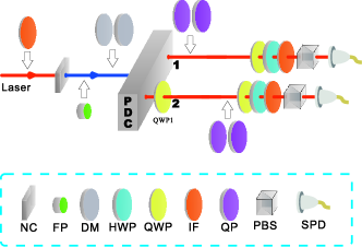
Figure 1: Experimental setup. Maximally entangled photon pairs are generated by parametric down conversion (PDC) with an ultraviolet (UV) pump pulse whose spectral width can be controlled. Then a series of quartz plates are added in arm $1$ and arm $2$ to realize the local dephasing channels. The final two-photon polarization state is analyzed by state tomography. Key to the components: NC – nonlinear crystal, FP – Fabry-Pérot cavity, DM – dispersion medium, HWP – half wave plate, QWP – quarter wave plate, IF – interference filter, QP – quartz plate, PBS – polarizing beamsplitter, and SPD – single photon detector.

Any pure initial state for the polarization degrees of freedom of the photon pair, which forms our bipartite open system, can be written as $\mathinner{|{\psi_{12}}\rangle}=a\mathinner{|{HH}\rangle}+b\mathinner{|{HV}\rangle}+c\mathinner{|{VH}\rangle}+d\mathinner{|{VV}\rangle}$. The total system initial states are assumed to be product states

$$\mathinner{|{\Psi(0)}\rangle}=\mathinner{|{\psi_{12}}\rangle}\otimes\int d\omega_{1}d\omega_{2}\,g(\omega_{1},\omega_{2})\mathinner{|{\omega_{1},\omega_{2}}\rangle},$$

where $g(\omega_{1},\omega_{2})$ is the probability amplitude for the photon in arm $1$ to have frequency $\omega_{1}$ and for the photon in arm $2$ to have frequency $\omega_{2}$, with the corresponding joint probability distribution $P(\omega_{1},\omega_{2})=|g(\omega_{1},\omega_{2})|^{2}$.

Open system dynamics

The time evolution of the open system can be represented by means of the dynamical map $\Phi^{t}_{12}$ Breuer2007 which maps the initial polarization state $\rho_{12}(0)=\mathinner{|{\psi_{12}}\rangle}\mathinner{\langle{\psi_{12}}|}$ to the polarization state state $\rho_{12}(t)=\Phi^{t}_{12}\big{(}\rho_{12}(0)\big{)}$ at time $t$. Calculating the total system time evolution and taking the trace over the environment yields Laine11

$$\rho_{12}(t)=\left(\begin{array}[]{cccc}|a|^{2}&ab^{*}\kappa_{2}(t)&ac^{*}\kappa_{1}(t)&ad^{*}\kappa_{12}(t)\\ ba^{*}\kappa_{2}^{*}(t)&|b|^{2}&bc^{*}\Lambda_{12}(t)&bd^{*}\kappa_{1}(t)\\ ca^{*}\kappa_{1}^{*}(t)&cb^{*}\Lambda_{12}^{*}(t)&|c|^{2}&cd^{*}\kappa_{2}(t)\\ da^{*}\kappa_{12}^{*}(t)&db^{*}\kappa_{1}^{*}(t)&dc^{*}\kappa_{2}^{*}(t)&|d|^{2}\end{array}\right).$$ (1)

The dynamics represents a pure dephasing process whose decoherence functions can be expressed completely in terms of the Fourier transform of the joint probability distribution

$$G(t_{1},t_{2})=\int d\omega_{1}d\omega_{2}P(\omega_{1},\omega_{2})e^{-i\Delta n(\omega_{1}t_{1}+\omega_{2}t_{2})}$$ (2)

as $\kappa_{1}(t)=G(t_{1},0)$, $\kappa_{2}(t)=G(0,t_{2})$, $\kappa_{12}(t)=G(t_{1},t_{2})$ and $\Lambda_{12}(t)=G(t_{1},-t_{2})$, where $\Delta n=n_{V}-n_{H}$ denotes the birefringence. The function $\kappa_{i}(t)$ describes the decoherence of the polarization state of photon $i$ which is induced by the local coupling to its frequency environment caused by the quartz plate in arm $i$. This can be seen by taking the trace over the polarization state of photon 2 to obtain the polarization state of photon 1:

$$\rho_{1}(t)=\left(\begin{array}[]{cc}|a|^{2}+|b|^{2}&(ac^{*}+bd^{*})\kappa_{1}(t)\\ (ca^{*}+db^{*})\kappa_{1}^{*}(t)&|c|^{2}+|d|^{2}.\end{array}\right),$$

or by tracing over photon 1 to find the state of photon 2:

$$\rho_{2}(t)=\left(\begin{array}[]{cc}|a|^{2}+|c|^{2}&(ab^{*}+cd^{*})\kappa_{2}(t)\\ (ba^{*}+dc^{*})\kappa_{2}^{*}(t)&|b|^{2}+|d|^{2}\end{array}\right).$$

Nonlocal dynamical map

The nonlocal character of the dynamical map $\Phi_{12}^{t}$ is controlled by the decoherence functions $\kappa_{12}(t)$ and $\Lambda_{12}(t)$ in Eq. (1). As a matter of fact, the map $\Phi_{12}^{t}$ is a product of local dynamical maps, i.e., $\Phi_{12}^{t}=\Phi_{1}^{t}\otimes\Phi_{2}^{t}$ if and only if $\kappa_{12}(t)=\kappa_{1}(t)\kappa_{2}(t)$ and $\Lambda_{12}(t)=\kappa_{1}(t)\kappa^{*}_{2}(t)$. In particular, this implies that frequency correlations in the initial state do not influence the local dynamics of each photon and cannot be detected by observing the local polarization states. However, the evolution of the composite two-photon polarization state is determined by the frequency correlations in the environment which lead to memory effects and global non-Markovian dynamics. This also means that, counterintuitively, by adding degrees of freedom to an open system one can change its dynamics from the Markovian to the non-Markovian regime.

Trace distance dynamics

To quantify non-Markovianity we use the trace distance based measure BLP which is defined by $\mathcal{N}(\Phi)=\max_{\rho_{A,B}(0)}\int_{\sigma>0}dt\,\sigma(t,\rho_{A,B}(0))$. Here, $\sigma(t,\rho_{A,B}(0))=\frac{d}{dt}D(\rho_{A}(t),\rho_{B}(t))$ and the trace distance $D$ between two states $\rho_{A}$ and $\rho_{B}$ is given by $D(\rho_{A},\rho_{B})=\frac{1}{2}\textrm{tr}|\rho_{A}-\rho_{B}|$. The amount of non-Markovianity is therefore equal to the total increase of the trace distance during the time evolution and quantifies the total information flow from the environment to the system. This measure has been used recently in several theoretical and experimental contexts, see, e.g. Refs. Rebentrost ; Liu ; Paternostro ; Tang .

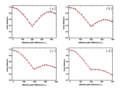
Figure 2: Trace distance dynamics for different values of the spectral width of the pump pulse. The widths and the amounts of non-Markovianity are: (a) $\delta=0.18\,\rm{nm}$, $\mathcal{N}=0.48$, (b) $\delta=0.52\,\rm{nm}$, $\mathcal{N}=0.23$, (c) $\delta=0.73\,\rm{nm}$, $\mathcal{N}=0.14$, (d) $\delta=1.89\,\rm{nm}$, $\mathcal{N}=0.02$. The $x$-axis represents time measured by the total effective path difference between the horizontal and vertical photons caused by quartz plates in arms $1$ and $2$ ($\lambda_{0}=780\,\rm{nm}$). The $y$-axis is the trace distance between the time-evolved initial open system states $|\psi_{12}^{+}\rangle$ and $|\psi_{12}^{-}\rangle$. We first add quartz plates in arm 1. When the total effective path difference between horizontal and vertical photons equals $199\lambda_{0}$, we add quartz plates in arm 2. The solid line shows the fit using the theoretical result of Eq. (3). The error bars are due to the counting statistics. See the Supplementary Information for more details on the counting statistics and the fitting of the theoretical curves.

For anticorrelated frequencies $\omega_{i}$ the pair of the Bell-states $|\psi_{12}^{\pm}\rangle=\left(|HH\rangle\pm|VV\rangle\right)/\sqrt{2}$ maximizes the increase of the trace distance and thus determines the non-Markovianity measure $\mathcal{N}$ Laine11 . These states are created by using spontaneous parametric down conversion as is illustrated in Fig. 1. A femtosecond pulse (the duration is about $150\,\rm{fs}$ and the operation wavelength is at $780\,\rm{nm}$, with a repetition rate of about $76\,\rm{MHz}$) generated from a Ti:sapphire laser is frequency doubled to pump two $1$mm-thick beamlike cut beta barium borate (BBO) crystals Niu creating the two-photon entangled state. With the help of QWP1 we can easily tune the entangled state between $\mathinner{|{\psi_{12}^{+}}\rangle}$ (QWP1 is set at $0^{\circ}$) and $\mathinner{|{\psi_{12}^{-}}\rangle}$ (QWP1 is set at $90^{\circ}$). The size of the anticorrelations between the photon frequencies is controlled in the experiment by the spectrum of the UV pump pulse. Since energy is conserved in the down conversion process, decreasing the spectral width of the pump pulse decreases the uncertainty of the sum of the frequencies of the photons, and hence increases the anticorrelation between the frequencies. We use four different pulse widths as described in more detail in the Methods Section. It is also worth noting that even though our experimental setup is based on downconversion, which is a commonly used tool to prepare specific two-photon states in quantum optical experiments, the physical phenomena that we describe and realize experimentally was theoretically predicted only very recently Laine11 .

Figure 3: Trace distance dynamics of the open system with different dispersions of the pump pulse. The quartz plate on the path of the pump pulse has thickness (a) $0$ (b) $13.19\,\rm{mm}$ (c) $39.57\,\rm{mm}$. In all cases $K=-0.55$ and the measured values of non-Markovianity are $\mathcal{N}=0.14,0.13,0.13$. The trace distance dynamics remains the same irrespective of the character of the correlations. See the Methods Section for further details.

Assuming a Gaussian joint frequency distribution $P(\omega_{1},\omega_{2})$ with identical single frequency variance $C$ and correlation coefficient $K$, the time evolution of the trace distance corresponding to the optimal Bell-state pair is found to be Laine11

$$D(t)=\exp\left[-\frac{1}{2}\Delta n^{2}C\left(t_{1}^{2}+t_{2}^{2}-2|K|t_{1}t_{2}\right)\right].$$ (3)

For uncorrelated photon frequencies, i.e. for uncorrelated local environments we have $K=0$ and the trace distance decreases monotonically, corresponding to Markovian dynamics. However, as soon as the frequencies are anticorrelated, $K<0$, the trace distance is non-monotonic which signifies quantum memory effects and non-Markovian behavior.

Consecutive interactions with local environments

In our first experiment the local decoherence induced by the quartz plates in arm $1$ and arm $2$ act consecutively, and we change the size of the initial correlations between the local reservoirs by tuning the spectral width of the pump pulse. The results for the open system’s trace distance dynamics are displayed in Fig. 2, which shows how the initial environmental correlations induce and influence the quantum non-Markovianity. First, when only the quartz plate in arm $1$ is active, the trace distance decreases monotonically demonstrating that information flows continuously from the system to the environment. When subsequently the quartz plate in arm $1$ becomes inactive and the quartz plate in arm $2$ active, the trace distance increases again highlighting non-Markovian behavior and a reversed flow of information from the environment back to the open system. It is important to note that this increase of the trace distance implies a revival of the entanglement between the photon polarizations. Whilst there exists earlier literature, e.g., on how the entanglement is transferred from the open system to the environment Lopez2008 , or on entanglement dynamics when the qubits interact with local non-Markovian reservoirs Bellomo , our results are fundamentally different. We demonstrate that the entanglement can revive due to the nonlocal character of the dynamical map despite of the fact that the local interaction of the qubits with their environments is completely Markovian. A further important aspect of the experimental scheme is that it enables to measure the frequency correlation coefficient $K$ of the photon pairs by fitting the theoretical prediction of Eq. (3) to the experimental data. The fits shown in Fig. 2 corresponding to panels (a)-(d) yield the values $K=-0.92$, $-0.66$, $-0.55$, and $-0.17$. Thus we see that the open system (polarization degrees of freedom) functions as a quantum probe which allows us to gain nontrivial information on the correlations in the environment (frequency degrees of freedom). To the best of our knowledge, our results present the first quantitative measurement of the correlation coefficient without reconstructing the joint frequency distribution.

Classical vs. quantum initial correlations between the local environments

The open system dynamics of Eq. (1) depends solely on the decoherence functions $\kappa_{1}$, $\kappa_{2}$, $\kappa_{12}$ and $\Lambda_{12}$ which in turn are completely determined by the Fourier transform (2) of the joint frequency distribution $P(\omega_{1},\omega_{2})$. Therefore, also the dynamical map of the open system depends only on $P(\omega_{1},\omega_{2})$ and not on the probability amplitudes $g(\omega_{1},\omega_{2})$. This fact leads to the conclusion that the nonlocal memory effects, and the revival of entanglement observed above, do not depend on the specific phase relations between different frequency components, and consequently, whether the initial frequency correlations between the photons are of quantum or classical character. To test experimentally whether the nature of the correlations plays a role in inducing the memory effects, we insert quartz plates also on the path of the pump pulse, thereby changing the dispersion relations of the pump pulse while keeping fixed the correlation coefficient $K$. The results in Fig. 3 show that the trace distance dynamics remains the same in this case and only depends on the correlation coefficient $K$ of the photon frequencies. Thus we see that nonlocal memory effects and the revival of the entanglement between the polarization states of the photons can be induced by purely classical correlations between local environments of the open system.

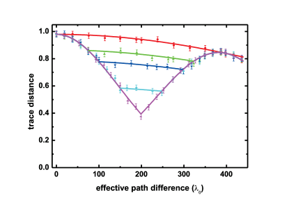
Figure 4: Trace distance dynamics for five different quartz plate configurations and a fixed correlation coefficient of $K=-0.92$. For all curves the maximal length of the quartz plates in both arms is $199\lambda_{0}$, giving a maximal total effective path difference of $398\lambda_{0}$. From top to bottom, the curves show the results for the cases, when we start to add quartz plates to arm $2$ when the length of the plate in arm $1$ has reached the length of $0,75,100,150,199\lambda_{0}$ respectively, see the Methods Section for details. Hence, in the top curve the quartz plates are added simultaneously to both arms while in the bottom curve they act consecutively. The results demonstrate that the final state is the same while in terms of the information flow the behaviour is completely different. For the top (red) curve information flows slowly out of the system with a small rate and, in fact, the decoherence would completely halt in the ideal ideal case of fully anticorrelated frequencies ($K=-1.0$). In the other extreme, for the bottom (violet) curve information first flows out of the system with a high rate and later on returns back nearly completely indicating strong memory effects. The solid lines are fits on the basis of Eq. (3), see the Methods Section for details

Different interaction configurations

In the previous experiments the local dephasing environments acted consecutively. In our final experimental series we reposition the quartz plates in arm 2 so that eventually the dephasing is active simultaneously in both arms (see the Methods Section). The results are shown in Fig. 4. We observe that the final state of the open system is always the same when the total effective path difference is equal to $398\lambda_{0}$. However, the amount of non-Markovianity and the flow of information from the environment to the open system decreases with increasing overlap of the action of the quartz plates. This demonstrates that initial correlations between the local environments and the reordering of the quartz plates allow to engineer the information flow between local systems while keeping fixed the final state. It is also important to note that when the local dephasing channels act simultaneously on our open bipartite system (the top red curve in Fig. 4), the initial correlations between the composite environments protect the entanglement between the qubits. One can see this also from Eq. (3) which shows that for $t_{1}=t_{2}$ and $K=-1$ the trace distance remains constant and that there is thus no outflow of information from the system for the considered Bell-states.

Discussion

We have realized nonlocal quantum dynamical maps of a photonic system and demonstrated experimentally how initial quantum or even classical correlations between the local environments of a composite open system induce nonlocal memory effects. While the global dynamics of the open system is non-Markovian, its local subsystems behave perfectly Markovian. The observation of the open system dynamics yields also important information about the environment. In fact, we have seen that a measurement of the non-Markovian evolution of the two-photon polarization state leads to a novel method for the determination of the correlation coefficient of the photon frequencies. Thus, the open system dynamics can be viewed as a non-Markovian quantum probe which enables to extract nontrivial information on characteristic features of the environment. This fact as well as our demonstration that initial correlations in the environment can protect the entanglement within an open system, could find important applications in quantum technologies and control strategies, and in the development of novel diagnostics tools for complex quantum systems.

Methods

Controlling the widths of the pump pulse

The width of the pump spectrum controls the frequency anticorrelations between the pair of photons created in the down conversion process. By using filters and fused silica plates, we can control the width of the pump pulses which are depicted in Fig. 5. The laser source is filtered to $3\,\rm{nm}$ (FWHF) and then passes through the frequency doubler ($1.5\,\rm{mm}$ thick BiB₃O₄). Hence, the bandwidth of the UV pulse is about $0.52\,\rm{nm}$ as shown in Fig. 5 (b). To obtain a sharper spectrum, as shown in Fig. 5 (a), we insert a thin fused silica plate, which is $0.05\,\rm{mm}$ thick and coated with a partial reflecting coating on each side, with approximately $75$% at $390\,\rm{nm}$. For the spectra displayed in Fig. 5 (c) and (d), we have no filter before the doubler and no fused silica plate after the doubler, and for Fig. 5 (d) we also replace the doubler by a $0.3\,\rm{mm}$-thick BBO.

Counting statistics

The details of the counting statistics and pump power for the experimental results of Fig. 2 are as follows. For Fig. 2 (a) the pump power is about $2.4\,\rm{mW}$ and the total coincident count rate on the basis vectors HH, HV, VH, VV is about $18,000$ in $10$ seconds, (b) $10\,\rm{mW}$ and the rate is about $35,000$ in $4$ seconds, (c) $20\,\rm{mW}$ and the rate is about $35,000$ in $2$ seconds, and (d) $20\,\rm{mW}$ and rate is about $36,000$ in $4$ seconds. Please note that the coincident count rate always depends also on the bandwidth of UV pump source.

Fitting the experimental data

Employing Eq. (3), the theoretical fits of the experimental data presented in Figs. 2 and 3 have been carried out as follows. We first use the function $f(x)=A\exp\left(-Bx^{2}\right)$ to make a fit for the process when the quartz plates are added to arm 1. From this process, we can find $A$ and $B$ which agree with the experimental data. Then in the second part, when the quartz plate in arm 2 is active, we use the function $g(x)=A\exp\left[-B\left(199^{2}+(x-199^{2})-2|K|199(x-199)\right)\right]$. Here, $199$ corresponds to the effective path difference after the first quartz plate. Since $A$ and $B$ are determined by the first fit, we can easily determine $K$ from the second fit.

For Fig. 4, again keeping in mind Eq. (3), we can do the fitting in the following way. First, we use the functions $f(x)$ and $g(x)$ mentioned above to make a fit of the lowest curve and determine $A_{1}$, $B_{1}$, and $K_{1}$. Then we use a function $G(x)=A\exp\left[-B\left(x^{2}/2-|K|x^{2}/2\right)\right]$ to fit the top curve of the figure. From here, we determine $A_{2}$, $B_{2}$, and $K_{2}$. Then we determine $A_{0}=(A_{1}+A_{2})/2$, $B_{0}=(B_{1}+B_{2})/2$, and $K_{0}=(K_{1}+K_{2})/2$ which are then used to plot the functions $F(t_{1},t_{2})=A_{0}\exp\left[-B_{0}\left(t_{1}^{2}+t_{2}^{2}-2|K_{0}|t_{1}t_{2}\right)\right]$ in the figure.

Trace distance dynamics with different dispersions of the pump pulse

For the experimental results of Fig. 3, the FWHM of the pump pulse is about $0.73\,\rm{nm}$, the pump power is about $20\,\rm{mW}$, and the total coincident count rate on the basis vectors HH, HV, VH, VV is about $35,000$ in $2$ seconds.

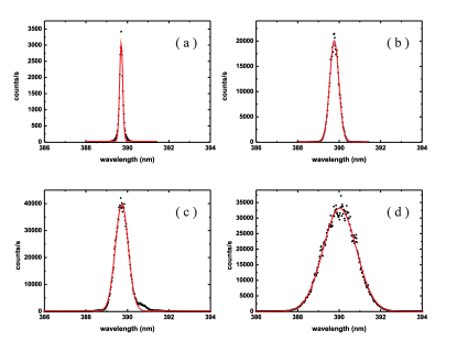
Figure 5: The frequency spectra of the ultra-violet (UV) pump pulses used for the down conversion process. Full widths at half maximum (FWHM) of the pulse spectra are (a) $\delta=0.18\,\rm{nm}$, (c) $\delta=0.52\,\rm{nm}$, (c) $\delta=0.73\,\rm{nm}$, and (d) $\delta=1.89\,\rm{nm}$. The solid lines represent Gaussian fits of the experimental data.

Quartz plate configurations

Figure 6 shows the five different quartz plate configurations used for Fig. 4. To obtain the data of Fig. 4, the FWHM of the UV pulse is about $0.18\,\rm{nm}$, the pump power is about $2.4\,\rm{mW}$, and the total coincident count rate on the basis vectors HH, HV, VH, VV is about $18,000$ in $10$ seconds.

Figure 6: The schematic view of the different quartz plate configurations. The configurations from (a) to (e) correspond to the curves of Fig. 4 from top to bottom. For all cases the maximal length of the quartz plates in both arms is $199\lambda_{0}$, giving a maximal total effective path difference of $398\lambda_{0}$. We start to add quartz plates to arm $2$ when the length of the plate in arm $1$ has reached the length of (a) $0$, (b) $75\lambda_{0}$, (c) $100\lambda_{0}$, (d) $150\lambda_{0}$, and (e) $199\lambda_{0}$.

Author Contributions

B.-H.L., D.-Y.C, Y.-F.H., C.-F.L., and G.-C.G. planned, designed and implemented the experiments. C.-F.L, G.-C. G., E.-M.L., H.-P.B., and J.P. carried out the theoretical analysis and developed the interpretation. B.-H.L., C.-F.L., E.-M.L, H.-P.B., and J.P. wrote the paper and all authors discussed the contents.

Author Information

The authors declare that they have no competing financial interests. Correspondence and requests for materials should be addressed to C.-F.L. or J.P.

References

- (1) Verstraete, F., Wolf, M. M. & Cirac, J. I. Quantum computation and quantum-state engineering driven by dissipation. Nature Physics 5, 633-636 (2009).
- (2) Diehl, S. et al. Quantum states and phases in driven open quantum systems with cold atoms. Nature Physics 4, 878-883 (2008).
- (3) Krauter, H. et al. Entanglement generated by dissipation and steady state entanglement of two macroscopic objects. Phys. Rev. Lett. 107, 080503 (2011).
- (4) Cho, J., Bose, S. & Kim, M. S. Optical pumping into many-body entanglement. Phys. Rev. Lett. 106, 020504 (2011).
- (5) Barreiro, J. T. et al. An open-system quantum simulator with trapped ions. Nature 470, 486-491 (2011).
- (6) Liu, B.-H. et al. Experimental control of the transition from Markovian to non-Markovian dynamics of open quantum system. Nature Physics 7, 931-934 (2011).
- (7) Piilo, J., Maniscalco, S., Härkönen, K. & Suominen, K.-A. Non-Markovian quantum jumps. Phys. Rev. Lett. 100, 180402 (2008).
- (8) Breuer, H.-P. & Vacchini, B. Quantum semi-Markov processes. Phys. Rev. Lett. 101, 140402 (2008).
- (9) Wolf, M. M., Eisert, J., Cubitt, T. S. & Cirac, J. I. Assessing Non-Markovian Quantum Dynamics. Phys. Rev. Lett. 101, 150402 (2008).
- (10) Shabani, A. & Lidar D. A. Vanishing quantum discord is necessary and sufficient for completely positive maps. Phys. Rev. Lett. 102, 100402 (2009).
- (11) Breuer, H.-P., Laine, E.-M. & Piilo, J. Measure for the Degree of Non-Markovian Behavior of Quantum Processes in Open Systems. Phys. Rev. Lett. 103, 210401 (2009).
- (12) Rivas, A., Huelga, S. F. & Plenio, M. B. Entanglement and Non-Markovianity of Quantum Evolutions. Phys. Rev. Lett. 105, 050403 (2010).
- (13) Chruściński, D. & Kossakowski, A. Non-Markovian Quantum Dynamics: Local versus Nonlocal Phys. Rev. Lett. 104, 070406 (2010).
- (14) Bellomo, B., Lo Franco, R. & Compagno, G. Non-Markovian Effects on the Dynamics of Entanglement. Phys. Rev. Lett. 99, 160502 (2007).
- (15) Rebentrost, P. & Aspuru-Guzik, A. Exciton-phonon information flow in the energy transfer process of photosynthetic complexes. J. Chem. Phys. 134, 101103 (2011).
- (16) Laine, E.-M., Breuer, H.-P., Piilo J., Li, C.-F. & Guo, G.-C. Nonlocal memory effects in the dynamics of open quantum systems. Phys. Rev. Lett. 108, 210402 (2012).
- (17) Breuer, H.-P & Petruccione, F. The Theory of Open Quantum Systems (Oxford University Press, Oxford, 2007).
- (18) Tony J. G. Apollaro, T. J. G., Di Franco, C., Plastina, F. & Paternostro, M. Memory-keeping effects and forgetfulness in the dynamics of a qubit coupled to a spin chain. Phys. Rev. A 83, 032103 (2011).
- (19) Tang, J.-S. et al. Measuring non-Markovianity of processes with controllable system-environment interaction. Europhys. Lett. 97, 10002 (2012).
- (20) Niu, X. L., Huang, Y. F., Xiang, G. Y., Guo, G. C. & Ou, Z. Y. Beamlike high-brightness source of polarization-entangled photon pairs. Opt. Lett. 33, 968 (2008).
- (21) Lòpez, C. E., Romero, G., Lastra, F., Solano, E. & Retamal, J. C. Sudden birth versus sudden death of entanglement in multipartite systems. Phys. Rev. Lett. 101, 080503 (2008).