On the effect of ghost force in the quasicontinuum method: Dynamic problems in one dimension

Abstract

Numerical error induced by the “ghost forces” in the quasicontinuum method is studied in the context of dynamic problems. The error in the ${W}^{1,\infty}$ norm is analyzed for the time scale $\mathcal{O}(\varepsilon)$ and the time scale $\mathcal{O}(1)$ with $\varepsilon$ being the lattice spacing.

1 Introduction

The present paper is mainly concerned with the error produced by the ghost forces in quasicontinuum (QC) type of multiscale coupling methods for crystalline solids. In these methods, one reduces the degrees of freedom of an atomic level description by replacing part of the system with continuum mechanics models [31, 2, 15, 20, 30]. Such integrated methods have been very useful in studying mechanical properties of lattice defects. It allows one to simulate a relatively large system while still able to keep the atomistic description around critical areas, such as crack tips and dislocations cores. These methods have also drawn a great deal of attention from numerical analysts. We refer to [18, 11, 10, 22, 5, 6, 28, 25] and references therein for a partial list of the representative work. Nevertheless, many challenges in the analysis of these methods still remain. Examples include high-dimensional problems, systems with line or wall defects, and solutions near bifurcation points. We refer to [19, 26] for a review of the state-of-art of this field. A critical issue that arises in the numerical analysis is the ghost force, which is the non-zero forces on the atoms near the interface at the equilibrium state [30]. For statics problems, the elimination of ghost forces has been a necessary ingredient to achieve uniform accuracy [10, 25].

In the static case, the QC method couples a molecular statics model to the Cauchy-Born elasticity model. For one-dimensional models, the influence of ghost forces has been explicitly characterized in [21, 22, 5]. They found that the ghost force may lead to an $\mathcal{O}(1)$ error for the gradient of the solution, and the width of the resulting interfacial layer is of the size $\mathcal{O}(\varepsilon\lvert\ln\varepsilon\rvert)$, where $\varepsilon$ is the equilibrium bond length. The influence of the ghost force for a two-dimensional model with planar interface has recently been studied in [4]. It was found that the ghost forces still lead to an $\mathcal{O}(1)$ error for the gradient of the solution, while the interfacial layer caused by the ghost force is of the size $\mathcal{O}(\sqrt{\varepsilon})$, which is much wider than that of the one-dimensional problems.

The QC method can be extended to dynamic problems using the coarse-grained energy and the Hamilton’s principle [29, 27]. The dynamic QC method couples an elastodynamics model with a molecular dynamics model. Many dynamic coupling methods with similar goals have been developed [1, 2, 8, 7, 9, 17, 32, 33, 35, 36] ever since. However, very little has been done to address the stability and accuracy of these methods. Most numerical studies have been focused on the artificial reflections at the interface. The reflection is caused by the drastic change in the dispersion relation across the interface, which is often due to the difference between the mesh size in the continuum region and the lattice spacing in the molecular dynamics model. The reflection can be studied by considering an incident wave packet traveling toward the interface and examine the amplitude of the reflected waves. The issue of ghost forces, however, has not yet been addressed.

The purpose of this paper is to study the effect of ghost forces in the context of dynamic problems. Motivated by the results in the static case, we expect that ghost forces will continue to play an important role in dynamic coupling models. To focus primarily on the issue of ghost forces, we consider the dynamic model [29, 27] derived from the original QC method when the mesh size coincides with the lattice spacing. In addition, the initial displacement is given by a uniform deformation. This allows us to compute the error caused only by the ghost forces. The error will be studied in the $W^{1,\infty}$-norm as in the static problem [21, 5, 22, 4]. Our study shows that the error, which is initially zero, grows very quickly, and already becomes $\mathcal{O}(1)$ at the time scale $\mathcal{O}(\varepsilon)$ . The error exhibits fast oscillations, with amplitude on the order of $\varepsilon$. On the time scale $\mathcal{O}(1)$, which is typically the time scale of interest, the amplitude of the oscillations grows, and it is bounded by an $\mathcal{O}(\sqrt{\varepsilon})$ quantity. The average of the oscillations has a peak at the interface. In contrast to the static case, where the error is mainly concentrated at the interface, the error in the dynamic case is observed in the entire domain on the time scale $\mathcal{O}(1)$. These observations are quite different from those of wave reflections, and it indicates that the effect of ghost forces is a separate numerical issue.

The rest of the paper is organized as follows. In Section 2 we describe the one-dimensional atomistic model and the derivation of the QC model, and briefly demonstrate the appearance of the ghost forces. In Section 3 we show results from several numerical tests. They provide some insight into the evolution of the error. The next three sections are devoted to the analysis of the error for short and long time scales. We draw some conclusions in the last section.

2 Motivation and the Formulation of the Problem

As in [12], we consider the dynamic problem of a one-dimensional chain of atoms. The interatomic interaction is assumed to be among the nearest and the next nearest neighbors. Let $x$ be the reference position of an atom, and $\widetilde{y}(x,t)$ be the current position at time $t$. The equations of motion for the atoms in the chain read,

$$\left\{\begin{aligned} \ddot{\widetilde{y}}(x,t)-\mathcal{L}_{\text{at}}[\widetilde{y}](x,t)&=0,\qquad x\in\mathbb{L},\\ \widetilde{y}(x,0)&=x,\;\dot{\widetilde{y}}(x,0)=x,\\ \widetilde{y}(x,t)-x&\;\text{is periodic with period}\;1.\end{aligned}\right.$$ (2.1)

Here, we have set the mass to unity, and $\mathbb{L}\equiv\{j\varepsilon,j\in\mathbb{N}\}\cap(-1/2,1/2)$ with $\varepsilon$ being the lattice parameter. The operator $\mathcal{L}_{\text{at}}$ is defined as

$$\mathcal{L}_{\text{at}}[z](x,t) \equiv\varepsilon^{-2}\bigl{[}\kappa_{2}z(x-2\varepsilon,t)+\kappa_{1}z(x-\varepsilon,t)+\kappa_{1}z(x+\varepsilon,t)+\kappa_{2}z(x+2\varepsilon,t)$$

$$\phantom{\equiv\varepsilon^{-2}\bigl{[}}\quad-2(\kappa_{1}+\kappa_{2})z(x,t)\bigr{]}.$$ (2.2)

Since the issue of ghost force arises even for harmonic interaction, we consider here a linear model, which can be considered as a harmonic approximation of a fully nonlinear model. In (2), $\kappa_{1}$ and $\kappa_{2}$ are the force constants computed from an interatomic potential. For example, for a pair potential, the energy is given by

$$E=\sum_{x}\Biggl{[}\varphi\left(\frac{y(x+\varepsilon)-y(x)}{\varepsilon}\right)+\varphi\left(\frac{y(x+2\varepsilon)-y(x)}{\varepsilon}\right)\Biggr{]}.$$

Direct calculation yields

$$\kappa_{1}=\varphi^{\prime\prime}(1),\;\kappa_{2}=\varphi^{\prime\prime}(2).$$

One commonly used model is the Lennard-Jones potential [16]:

$$\varphi(r)=\left(\sigma/r\right)^{12}-\left(\sigma/r\right)^{6}.$$

If only the nearest and the next nearest neighborhood interactions are considered, the lattice parameter is given by

$$\varepsilon=2^{1/6}\left(\dfrac{1+2^{-12}}{1+2^{-6}}\right)^{1/6}\sigma.$$

In this case, the force constants are

$$\kappa_{1}=156C^{2}-42C\approx 18.886\qquad\text{and}\qquad\kappa_{2}=2^{-6}(156C^{2}2^{-6}-42C)\approx-0.323,$$

where $C=(1+2^{-6})/[2(1+2^{-12})]$. The above formula has also appeared in [13]. Notice that the second force constant is negative, but it is much smaller than the first force constant in magnitude.

With the harmonic approximation, the potential energy takes the form of

$$E=\sum_{x}\Biggl{[}\frac{\kappa_{1}}{2}\left(\frac{y(x+\varepsilon)-y(x)}{\varepsilon}\right)^{2}+\frac{\kappa_{2}}{2}\left(\frac{y(x+2\varepsilon)-y(x)}{\varepsilon}\right)^{2}\Biggr{]}.$$

The dynamic model (2.1) can be derived from this energy using Hamilton’s principle. Notice that the energy can be divided into the energy at each atom site: i.e. $E=\sum_{x}E(x)$, in which

$$E(x) =\frac{\kappa_{2}}{4}\left(\frac{y(x+2\varepsilon)-y(x)}{\varepsilon}\right)^{2}+\frac{\kappa_{1}}{4}\left(\frac{y(x+\varepsilon)-y(x)}{\varepsilon}\right)^{2}$$

$$\quad+\frac{\kappa_{1}}{4}\left(\frac{y(x)-y(x-\varepsilon)}{\varepsilon}\right)^{2}+\frac{\kappa_{2}}{4}\left(\frac{y(x)-y(x-2\varepsilon)}{\varepsilon}\right)^{2}.$$

In the QC method, one defines a local region where the atomistic model is approximated by the Cauchy-Born elasticity model [3]. One also defines a nonlocal region where the atomistic description is kept. Without loss of generality, we assume that the interface is located at $x=0$ and the nonlocal region is in the domain $x<0$. We further assume that the mesh size is equal to the lattice parameter to primarily focus on the effect of ghost forces. The Cauchy-Born approximation of the energy in the local region is given by

$$E_{{\rm CB}}(x)=\frac{\kappa_{1}+4\kappa_{2}}{4}\left(\frac{y(x+\varepsilon)-y(x)}{\varepsilon}\right)^{2}+\frac{\kappa_{1}+4\kappa_{2}}{4}\left(\frac{y(x)-y(x-\varepsilon)}{\varepsilon}\right)^{2}.$$

At the interface $x=0$, the energy takes a mixed form:

$$E(0) =\dfrac{\kappa_{2}}{4}\left(\dfrac{y(x)-y(x-2\varepsilon)}{\varepsilon}\right)^{2}+\dfrac{\kappa_{1}}{4}\left(\frac{y(x)-y(x-\varepsilon)}{\varepsilon}\right)^{2}$$

$$\quad+\dfrac{\kappa_{1}+4\kappa_{2}}{4}\left(\dfrac{y(x+\varepsilon)-y(x)}{\varepsilon}\right)^{2}.$$

With such energy summation rule, we may write the QC approximation of $\mathcal{L}_{\text{at}}$ as $\mathcal{L}_{\text{qc}}$, with $\mathcal{L}_{\text{qc}}$ given below. For $x\leq-2\varepsilon$,

$$\mathcal{L}_{\text{qc}}[z](x,t) \equiv\varepsilon^{-2}\bigl{[}\kappa_{2}z(x-2\varepsilon,t)+\kappa_{1}z(x-\varepsilon,t)+\kappa_{1}z(x+\varepsilon,t)+\kappa_{2}z(x+2\varepsilon,t)$$

$$\phantom{\equiv\varepsilon^{-2}\bigl{[}}\quad-2(\kappa_{1}+\kappa_{2})z(x,t)\bigr{]},$$

and for $x\geq 2\varepsilon$,

$$\mathcal{L}_{\text{qc}}[z](x,t)=\mathcal{L}_{\text{CB}},\;\mathcal{L}_{\text{CB}}\equiv\varepsilon^{-2}(\kappa_{1}+4\kappa_{2})[z(x-\varepsilon,t)-2z(x,t)+z(x+\varepsilon,t)].$$

This is exactly the operator corresponding to the Cauchy-Born approximation.

At the interface, we have for $x=-\varepsilon$,

$$\mathcal{L}_{\text{qc}}[z](x,t) \equiv\varepsilon^{-2}\bigl{[}\kappa_{2}z(x-2\varepsilon,t)+\kappa_{1}z(x-\varepsilon,t)+\kappa_{1}z(x+\varepsilon,t)+\dfrac{\kappa_{2}}{2}z(x+2\varepsilon,t)$$

$$\phantom{\equiv\varepsilon^{-2}\bigl{[}}\quad-(2\kappa_{1}+3\kappa_{2}/2)z(x,t)\bigr{]},$$

for $x=0$,

$$\mathcal{L}_{\text{qc}}[z](x,t) \equiv\varepsilon^{-2}\Bigl{[}\kappa_{2}z(x-2\varepsilon,t)+\kappa_{1}z(x-\varepsilon,t)+(\kappa_{1}+4\kappa_{2})z(x+\varepsilon,t)$$

$$\phantom{\equiv\varepsilon^{-2}\Bigl{[}}\quad-(2\kappa_{1}+5\kappa_{2})z(x,t)\Bigr{]},$$

and for $x=\varepsilon$,

$$\mathcal{L}_{\text{qc}}[z](x,t) \equiv\varepsilon^{-2}\Bigl{[}\dfrac{\kappa_{2}}{2}z(x-2\varepsilon,t)+(\kappa_{1}+4\kappa_{2})z(x-\varepsilon,t)+(\kappa_{1}+4\kappa_{2})z(x+\varepsilon,t)$$

$$\phantom{\varepsilon^{-2}\Bigl{[}}\qquad-(2\kappa_{1}+17\kappa_{2}/2)z(x,t)\Bigr{]}.$$

Using the Hamilton’s principle, we write the QC model as

$$\left\{\begin{aligned} \ddot{\widetilde{y}}(x,t)-\mathcal{L}_{\text{qc}}[\widetilde{y}](x,t)&=0,\qquad x\in\mathbb{L},\\ \widetilde{y}(x,0)=x,\;\dot{\widetilde{y}}(x,0)&=x,\\ \widetilde{y}(x,t)-x\;&\text{is periodic with period}\;1.\end{aligned}\right.$$ (2.3)

The initial and boundary conditions have been chosen as a uniform deformation in order to identify the effect of the ghost force. We will compute the deviation of the solution away from the equilibrium. For this purpose, we define the error $y(x,t)=\widetilde{y}(x,t)-x$, and we have,

$$\ddot{y}(x,t)-\mathcal{L}_{\text{qc}}[y](x,t) =\ddot{\widetilde{y}}(x,t)-\mathcal{L}_{\text{qc}}[\widetilde{y}-x](x,t)$$ (2.4)

$$=\mathcal{L}_{\text{qc}}[x](x,t)\equiv f(x,t),$$

with $f$ given explicitly by

$$f(x,t)=\left\{\begin{aligned} 0\quad&\text{if\quad}\lvert x\rvert\geq 2\varepsilon,\\ -\dfrac{\kappa_{2}}{\varepsilon}\quad&\text{if\quad}x=-\varepsilon,\\ \dfrac{2\kappa_{2}}{\varepsilon}\quad&\text{if\quad}x=0,\\ -\dfrac{\kappa_{2}}{\varepsilon}\quad&\text{if\quad}x=\varepsilon.\end{aligned}\right.$$ (2.5)

The function $f(x,t)$ is precisely the ghost force. Since it is independent of the temporal variable, we denote it by $f(x)$ for simplicity. Finally, we supplement the above problem with the homogeneous initial condition and periodic boundary condition as

$$\left\{\begin{aligned} y(x,0)&=0\text{\quad and\quad}\dot{y}(x,0)=0,\qquad x\in\mathbb{L}.\\ y(x,t)&\;\text{is periodic with period\;}1.\end{aligned}\right.$$ (2.6)

3 Observations from Numerical Results

Since the operator $\mathcal{L}_{\text{qc}}$ coincides with $\mathcal{L}_{\text{CB}}$ in the local region, and with $\mathcal{L}_{\text{at}}$ in the nonlocal region, it is natural to look at models similar to (2.4), in which $\mathcal{L}_{\text{qc}}$ is replaced by either $\mathcal{L}_{\text{CB}}$ or $\mathcal{L}_{\text{at}}$ in the entire domain. Therefore, our numerical experiments are conducted for the following three models:

• Model I. $\mathcal{L}_{\text{qc}}$ is approximated by $\mathcal{L}_{\text{CB}}$: $\ddot{y}-\mathcal{L}_{\text{CB}}[y]=f.$

• Model II. $\mathcal{L}_{\text{qc}}$ is approximated by $\mathcal{L}_{\text{at}}$: $\ddot{y}-\mathcal{L}_{\text{at}}[y]=f.$

• Model III: The quasicontinuum model (2.4).

In all these models, we impose homogeneous initial condition and periodic boundary condition (2.6).

As an example, the force constants are obtained from the Morse potential [24]. In particular, we choose $\kappa_{1}=4.4753$ and $\kappa_{2}=0.4142$. All the simulations are performed in the domain $x\in[-1/2,1/2]$, and the ODEs are integrated using the Verlet’s method. Since all three models are Hamiltonian systems, this method is particularly suitable.

We first show the solutions computed from the three models at different time step. The results are shown in Fig. 1. For this set of numerical tests, we have chosen $\varepsilon=1/2000$. We observe that the error first developed at the interface, and then it starts to spread toward the local and nonlocal region for all three models. Another noticeable feature is that the error exhibits a peak at the interface, and the peak remains for all later time. At $t=1$, the error is observed in the entire domain.

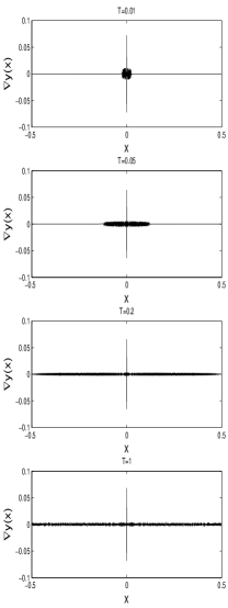
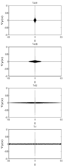
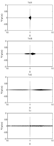
Fig. 1: The gradient of the error. Left to right: Solution computed from Model I, II and III. From top to bottom: The solutions at time $t=0.01,0.05,0.2\;\rm{and}\;1$.

Our main observations here can be summarized as following: (1) In the presence of ghost forces, the error grows very quickly. It reaches $\mathcal{O}(1)$ on the time scale of $\mathcal{O}(\varepsilon)$; (2) At the time scales of $t=\mathcal{O}(\varepsilon)$ and $t=\mathcal{O}(1)$, the solutions of all three models are qualitatively the same.

Next we monitor the solution for those atoms near the interface. In Fig. 2, we show the time history for those atoms. We observe that for most of the time, the error oscillates around certain constant values, and the constant values depend on the location of the atom. These constant values show a peak at the interface $x=0$.

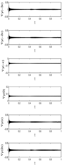
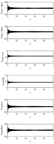
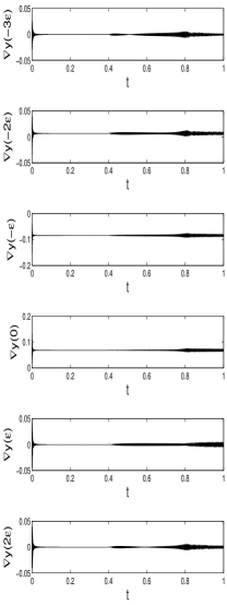
Fig. 2: The time history of the gradient of the error near the interface. Left to right: Solution computed from Model I, II and III. From top to bottom: The solutions near the interface: $x=-3\varepsilon$,$x=-2\varepsilon$,$x=-\varepsilon$,$x=0$,$x=\varepsilon$ and $x=2\varepsilon$.

In the last two figures, Fig. 3 and Fig. 4, we show the time history of the solution at the interface for various values of $\varepsilon$. The main observation is that the amplitude of the oscillation decrease as $\varepsilon$ gets small. However, the constant values around which the solutions oscillate do not change as $\varepsilon$ varies.

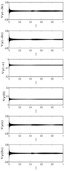
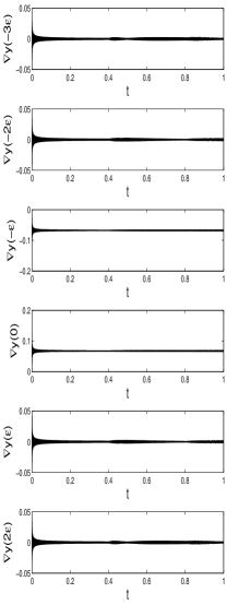
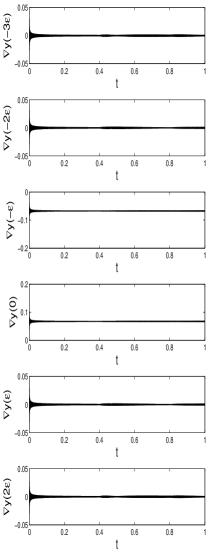
Fig. 3: The gradient of the error. The solutions are computed from Model I with different choice of $\epsilon$. Left to right: Solution computed for $\varepsilon=1/2000$, $\varepsilon=1/4000$ and $\varepsilon=1/8000$. From top to bottom: The solutions near the interface: $x=-3\varepsilon$, $x=-2\varepsilon$, $x=-\varepsilon$, $x=0$, $x=\varepsilon$ and $x=2\varepsilon$.

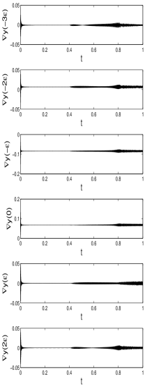
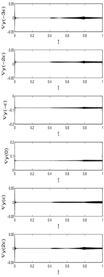
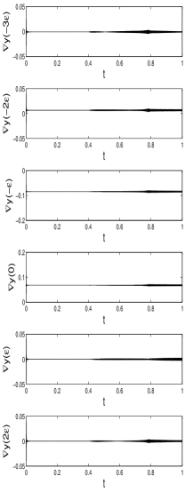
Fig. 4: The gradient of the error. The solutions are computed from Model III with different choices of $\varepsilon$. Left to right: Solution computed for $\varepsilon=1/2000$, $\varepsilon=1/4000$ and $\varepsilon=1/8000$. From top to bottom: The solutions near the interface: $x=-3\varepsilon$, $x=-2\varepsilon$, $x=-\varepsilon$, $x=0$, $x=\varepsilon$ and $x=2\varepsilon$.

4 Explicit Solutions for the Approximating Model

In view of the numerical results, it seems that the solution of model I bears similarity to the dynamical behavior of the original problem (2.4) on the time scale $\mathcal{O}(\varepsilon)$ and time scale $\mathcal{O}(1)$. Therefore we will turn to this model to study the effect of ghost forces. Model I is convenient to analyze, particularly because it admits explicit solutions of a simple form. Recall that in Model I, we solve the following problem,

$$\left\{\begin{aligned} \ddot{y}(x,t)-\mathcal{L}_{\text{CB}}[y](x,t)&=f(x),\qquad x\in\mathbb{L},\\ y(x,0)=0,\dot{y}(x,0)&=0,\\ y(x,t)&\text{\quad is periodic with period}\;1.\end{aligned}\right.$$ (4.1)

Without loss of generality, we let $\mathbb{L}=(-1/2,1/2]$ with $N$ atoms. We assume that $N$ is an even integer for technical simplicity. Obviously, $\varepsilon=1/N$. We will switch to the notation that,

$$w(n,t)=w(-1/2+n\varepsilon,t),\quad n=1,2,\cdots,N.$$ (4.2)

We now express the solution of (4.1) in an explicit form. To begin with, we consider the lattice Green’s function, which is defined as the solution of the following problem:

$$\left\{\begin{aligned} \ddot{G}(n,t)-\mathcal{L}_{\text{CB}}[G](n,t)&=0,\qquad n=0,\dots,N,\\ G(n,0)=0,\dot{G}(n,0)&=\delta_{n},\\ G(n,t)&=G(n+N,t).\end{aligned}\right.$$ (4.3)

Given this Green’s function, the solution of (4.1) is given by

$$y(n,t)=\int_{0}^{t}\left(\sum_{m=1}^{N}G(n-m,t-s)f(m)\right)\mathrm{d}s,$$

where $f$ is given by (2.5) under the transform (4.2). As a result, we have

$$\sum_{m=1}^{N}G(n-m,t)f(m)=\dfrac{\kappa_{2}}{\varepsilon}\left(2G(n-L,t)-G(n-L-1,t)-G(n-L+1,t)\right),$$

where we have set $L=N/2$.

By separation of variables, we have the following explicit form for the lattice Green’s function $G$:

$$G(n,t)=\dfrac{t}{N}+\dfrac{1}{N}\sum_{k=1}^{N-1}\dfrac{\sin[\omega_{k}t]}{\omega_{k}}\cos\dfrac{2kn\pi}{N},$$ (4.4)

with $\omega_{k}$ being the dispersion relation given by $\omega_{k}=(2/\varepsilon)\sqrt{\kappa_{1}+4\kappa_{2}}\sin(k\pi/N).$

Using $\sum_{m=1}^{N}f(m)=0$, we write

$$\sum_{m=1}^{N}G(n-m,t-s)f(m)=\dfrac{4\kappa_{2}}{N\varepsilon}\sum_{k=1}^{N-1}\dfrac{\sin[\omega_{k}(t-s)]}{\omega_{k}}\sin^{2}\dfrac{k\pi}{N}\cos\dfrac{2k\pi}{N}(n-L).$$

This leads to

$$y(n,t)=\int_{0}^{t}\left(\sum_{m=1}^{N}G(n-m,t-s)f(m)\right)\mathrm{d}s=\dfrac{\varepsilon}{N}\dfrac{2\kappa_{2}}{\kappa_{1}+4\kappa_{2}}\sum_{k=1}^{N-1}\sin^{2}\dfrac{\omega_{k}t}{2}\cos\dfrac{2k\pi}{N}(n-L).$$

Using the above expression we bound $y(n,t)$ as

$$\lvert y(n,t)\rvert\leq\dfrac{2\lvert\kappa_{2}\rvert}{\kappa_{1}+4\kappa_{2}}\varepsilon.$$ (4.5)

This estimate shows that the magnitude of the error $y(n,t)$ is as small as $\mathcal{O}(\varepsilon)$ for all $n$ and all time $t$. This in turn suggests that the error induced by the ghost force is small in the maximum norm, which is consistent with that of the static problem [5, 22, 4].

Next we consider the discrete gradient of the error. A direct calculation gives

$$Dy(n,t) \equiv\dfrac{y(n+1,t)-y(n,t)}{\varepsilon}$$

$$=-\dfrac{1}{N}\dfrac{4\kappa_{2}}{\kappa_{1}+4\kappa_{2}}\sum_{k=1}^{N-1}\sin\dfrac{2k\pi}{N}(n+1/2-L)\sin\dfrac{k\pi}{N}\sin^{2}\dfrac{\omega_{k}t}{2}.$$

Clearly we may write the above expression as

$$Dy(n,t)=-\dfrac{1}{N}\dfrac{4\kappa_{2}}{\kappa_{1}+4\kappa_{2}}\sum_{k=0}^{N}\sin\dfrac{2k\pi}{N}(n+1/2-L)\sin\dfrac{k\pi}{N}\sin^{2}\dfrac{\omega_{k}t}{2}.$$ (4.6)

It follows from the above expression that $Dy(n,t)$ is anti-symmetric in the sense of

$$Dy(n,t)=-Dy(N-n-1).$$

Therefore, we only consider the case $n\geq L$. By (4.5) we bound $Dy(n,t)$ trivially:

$$\lvert Dy(n,t)\rvert\leq\dfrac{4\lvert\kappa_{2}\rvert}{\kappa_{1}+4\kappa_{2}}.$$

This shows that $Dy(n,t)$ is uniformly bounded for all $n$ and all time $t$. In the next two sections, we seek for a refined pointwise estimate of $Dy(n,t)$ when $t$ is of $\mathcal{O}(1)$ and of $\mathcal{O}(\varepsilon)$. Notice that the same method can be employed to obtain a refined pointwise estimate of $y(n,t)$. We leave it to the interested readers.

5 Estimate of the error over long time

In this section, we estimate the error for $t=\mathcal{O}(1)$. By (4.6), we write $Dy(L,t)$ as

$$Dy(L,t)=-\dfrac{1}{N}\dfrac{4\kappa_{2}}{\kappa_{1}+4\kappa_{2}}\sum_{k=0}^{N}\sin^{2}\dfrac{k\pi}{N}\sin^{2}\dfrac{\omega_{k}t}{2}.$$

Using the identity

$$\sum_{k=0}^{N}\sin^{2}\dfrac{k\pi}{N}=\dfrac{N}{2}.$$

We write

$$Dy(L,t) =-\dfrac{1}{N}\dfrac{2\kappa_{2}}{\kappa_{1}+4\kappa_{2}}\sum_{k=0}^{N}\sin^{2}\dfrac{k\pi}{N}+\dfrac{1}{N}\dfrac{2\kappa_{2}}{\kappa_{1}+4\kappa_{2}}\sum_{k=0}^{N}\sin^{2}\dfrac{k\pi}{N}\cos(\omega_{k}t)$$

$$=-\dfrac{\kappa_{2}}{\kappa_{1}+4\kappa_{2}}+\dfrac{1}{N}\dfrac{2\kappa_{2}}{\kappa_{1}+4\kappa_{2}}\sum_{k=0}^{N}\sin^{2}\dfrac{k\pi}{N}\cos(\omega_{k}t),$$ (5.1)

When $n\neq L$, we use the fact that

$$\sum_{k=0}^{N}\sin\dfrac{2k\pi}{N}(n+1/2-L)\sin\dfrac{k\pi}{N}=0,$$

and we write the expression of $Dy(n,t)$ in (4.6) as

$$Dy(n,t)=\dfrac{1}{N}\dfrac{2\kappa_{2}}{\kappa_{1}+4\kappa_{2}}\sum_{k=0}^{N}\sin\dfrac{2k\pi}{N}(n+1/2-L)\sin\dfrac{k\pi}{N}\cos(\omega_{k}t),$$

which can be further decomposed into

$$Dy(n,t) =\dfrac{1}{N}\dfrac{\kappa_{2}}{\kappa_{1}+4\kappa_{2}}\sum_{k=0}^{N}\sin\dfrac{k\pi}{N}\biggl{\{}\sin\left(\omega_{k}t+\dfrac{2k\pi}{N}(n+1/2-L)\right)$$

$$\phantom{\dfrac{1}{N}\dfrac{\kappa_{2}}{\kappa_{1}+4\kappa_{2}}\sum_{k=0}^{N}\sin\dfrac{k\pi}{N}}\qquad-\sin\left(\omega_{k}t-\dfrac{2k\pi}{N}(n+1/2-L)\right)\biggr{\}}.$$ (5.2)

To bound $Dy(n,t)$, we need to estimate an exponential sum of the following form,

$$\sum_{k=0}^{N}e(f(k)),$$

where the shorthand $e(f(k))\equiv\exp(2\pi\imath f(k))$ is assumed. The basic tool that will be used is the truncated form of the Poisson summation formula due to Van der Corput [34]. The following form with an explicit estimate for the remainder term can be found in [14, Lemma 7].

Theorem 1.

(Truncated Poisson)  Let $f$ and $\phi$ be real-valued functions satisfying the following conditions on a closed interval $[a,b]$:

1. $f^{\prime\prime}$ and $\phi^{\prime}(x)$ are continuous;

2. $0<f^{\prime\prime}(x)\leq C_{0}$;

3. There are positive constants $H,U,\phi_{0},\phi_{1},\lambda$ such that $U\geq 1,0<b-a\leq\lambda U$ and

   $$\lvert\phi(x)\rvert\leq\phi_{0}H,\quad\lvert\phi^{\prime}(x)\rvert\leq\phi_{1}H/U.$$

For any $\Delta,0<\Delta<1$, the equation

$$\sum_{a<n\leq b}\phi(n)e(f(n))=\sum_{\alpha-\Delta\leq\nu\leq\beta+\Delta}\int_{a}^{b}\phi(x)e(f(x)-\nu x)\,\mathrm{d}x+\theta R$$ (5.3)

holds, where $\alpha=f^{\prime}(a)$, $\beta=f^{\prime}(b)$ and

$$R =(\phi_{0}+\lambda\phi_{1})H\Bigl{(}9.42+9C_{0}+12\Delta+\pi^{-1}\bigl{(}10\Delta^{-1}+2\ln\Delta^{-1}$$

$$\phantom{=(\phi_{0}+\lambda\phi_{1})H}\quad+4.5(1+\Delta)^{-1}-4.5\ln(1+\Delta)+6.5\ln(\beta-\alpha+2)\bigr{)}\Bigr{)}.$$

Here $\theta$ is a function such that $\lvert\theta\rvert\leq 1$.

The assumption $f^{\prime\prime}>0$ can be relaxed to either $f^{\prime\prime}\geq 0$ or $f^{\prime\prime}\leq 0$. In the latter case, the second condition is replaced by $-C_{0}\leq f^{\prime\prime}(x)\leq 0$.

5.1 The estimate for $Dy(N/2,t)$

To bound $Dy(N/2,t)$, we start with (5.1). Based on the above theorem, we transform the exponential sum in (5.1) to a shorter sum with a bounded remainder. To clarify the dependance of the constant, we denote

$$\gamma=t\sqrt{\kappa_{1}+4\kappa_{2}},$$

and assume that $1\leq\gamma\leq N$ since $t=\mathcal{O}(1)$ and $N\geq 2$. We also denote by $\lfloor\,p\,\rfloor$ the integer part of a real number $p$, and denote its fractional part by $\{\,p\,\}=p-\lfloor\,p\,\rfloor$.

Lemma 2.

Let $\phi(x)=\sin^{2}(\pi x/N)$ and $f(x)=\gamma/(\pi\varepsilon)\sin(\pi x/N)$. There holds

$$\dfrac{1}{N}\left\lvert\,\sum_{k=0}^{N}\phi(k)e(f(k))\,\right\rvert \leq\left\lvert\,\dfrac{2}{N}\sum_{\alpha-1/2\leq\nu\leq\gamma+1/2}\int_{0}^{N/2}\phi(x)e(f(x)-\nu x)\,\mathrm{d}x\,\right\rvert$$

$$\quad+C\varepsilon(1+\varepsilon\gamma+\log(\gamma+2)),$$ (5.4)

where $C$ is independent of $N,t$ and $\gamma$.

Proof.

It is easy to write the exponential sum into

$$\sum_{k=0}^{N}\phi(k)e(f(k))=2\sum_{k=0}^{N/2}\phi(k)e(f(k))-\phi(N/2)e(f(N/2)).$$

With such choice of $f$ and $\phi$, we have

$$a =0,b=N/2,\alpha=0,\beta=\gamma,$$

$$\phi_{0} =\phi_{1}=1,H=\pi,\lambda=1,U=N/2.$$

Setting $\Delta=1/2$ and using Theorem 1, we obtain

$$\dfrac{1}{N}\sum_{k=0}^{N/2}\phi(k)e(f(k))=\dfrac{1}{N}\sum_{\alpha-1/2\leq\nu\leq\gamma+1/2}\int_{0}^{N/2}\phi(x)e(f(x)-\nu x)\,\mathrm{d}x+\theta\dfrac{R}{N},$$

where

$$R=2\pi\Bigl{(}9.42+9\pi\gamma/N+6+\pi^{-1}\bigl{(}20+2\ln 2+3-4.5\ln(3/2)+6.5\ln(\gamma+2)\bigr{)}\Bigr{)}.$$

This immediately implies that there exists a constant $C$ such that

$$\lvert\theta R/N\rvert\leq C\varepsilon\left(1+\varepsilon\gamma+\ln(\gamma+2)\right).$$

We obtain (2) by combining the above two inequalities. ∎

Remark 3.

The choice of $\Delta$ is not unique. However, it cannot be too small. Otherwise, the remainder term blows up as $\Delta\to 0$.

To bound the shorter sum in (2), we shall rely on the following first derivative test.

Lemma 4 (First derivative test).

[23, Lemma 1, p. 47] Let $r(x)$ and $\theta(x)$ be real-valued functions on $[a,b]$ such that $r(x)$ and $\theta^{\prime}(x)$ are continuous. Suppose that $\theta^{\prime}(x)/r(x)$ is positive and monotonically increasing in this interval. If $0<\lambda_{1}\leq\theta^{\prime}(a)/r(a)$, then

$$\left\lvert\,\int_{a}^{b}r(x)e(\theta(x))\,\mathrm{d}x\,\right\rvert\leq\dfrac{1}{\pi\lambda_{1}}.$$

Remark 5.

If $\theta^{\prime}(x)/r(x)$ is negative and monotonically decreasing on $[a,b]$ and

$$\theta^{\prime}(a)/r(a)\leq\lambda_{1}<0,$$

then we obtain the same bound by taking complex conjugates. Moreover, if $\theta^{\prime}(x)/r(x)$ is monotone on $[a,b]$ and

$$\lvert\theta^{\prime}(x)/r(x)\rvert\geq\lambda_{1}>0\qquad x\in(a,b),$$

we obtain the same bound by combining the above two cases.

We write

$$\dfrac{1}{N}\int_{0}^{N/2}\phi(x)e(f(x)-\nu x)\,\mathrm{d}x=\dfrac{1}{\pi}\int_{0}^{\pi/2}\varphi(y)e\left(G_{\nu}(y)\right)\,\mathrm{d}y,$$

where $\varphi(y)=\sin^{2}y$, and $G_{\nu}(y)=(N/\pi)(\gamma\sin y-\nu y)$ for any $\nu\in\mathbb{N}$. We define $F_{\nu}(y)=G_{\nu}^{\prime}(y)/\varphi(y)$. By Lemma 2, it remains to estimate the integral $\int_{0}^{\pi/2}\varphi(y)e(G_{\nu}(y))\,\mathrm{d}y$ for $\nu=0,\cdots,\lfloor\,\gamma+1/2\,\rfloor$. The three cases $\nu=0,\nu=1,\cdots,\lfloor\,\gamma+1/2\,\rfloor-1$ and $\nu=\lfloor\,\gamma+1/2\,\rfloor$ will be treated separately in the following lemmas.

Lemma 6.

There holds

$$\left\lvert\,\int_{0}^{\pi/2}\varphi(y)e\left(G_{0}(y)\right)\,\mathrm{d}y\,\right\rvert\leq 2(N\gamma)^{-1/2}\;.$$ (5.5)

Proof.

For any $\delta\in(0,\pi/2)$ that will be determined later on, we have, for any $y\in(0,\pi/2-\delta)$,

$$F_{0}(y)\geq F_{0}(\pi/2-\delta)=\dfrac{N\gamma}{\pi}\dfrac{\sin\delta}{\cos^{2}\delta}\geq\dfrac{N\gamma}{\pi}\tan\delta\geq\dfrac{N\gamma\delta}{\pi},$$

where we have used the fact that $\tan x\geq x$ for $x\in[0,\pi/2]$. Using Lemma 4 with $\lambda_{1}=N\gamma\delta/\pi$, we obtain

$$\left\lvert\,\int_{0}^{\pi/2-\delta}\varphi(y)e\left(G_{0}(y)\right)\,\mathrm{d}y\,\right\rvert\leq\dfrac{1}{N\gamma\delta}.$$

The integral over the complementary portion of the interval can be bounded trivially:

$$\left\lvert\,\int_{\pi/2-\delta}^{\pi/2}\varphi(y)e\left(G_{0}(y)\right)\,\mathrm{d}y\,\right\rvert\leq\int_{\pi/2-\delta}^{\pi/2}\,\mathrm{d}y\leq\delta.$$

On adding the two estimates we deduce that

$$\left\lvert\,\int_{0}^{\pi/2}\varphi(y)e\left(G_{0}(y)\right)\,\mathrm{d}y\,\right\rvert\leq\dfrac{1}{N\gamma\delta}+\delta.$$

This is minimized by taking $\delta=(N\gamma)^{-1/2}\in(0,\pi/2)$, and we obtain (5.5). ∎

The second case is more involved since $F_{\nu}$ changes sign over $(0,\pi/2)$.

Lemma 7.

If $1\leq\nu<\gamma$, then

$$\left\lvert\,\int_{0}^{\pi/2}\varphi(y)e(G_{\nu}(y))\,\mathrm{d}y\,\right\rvert\leq\dfrac{3\pi}{\sqrt{N\gamma}}.$$ (5.6)

Proof.

For $1\leq\nu<\gamma$, there exists $y_{\nu}\in(0,\pi/2)$ such that $F_{\nu}(y_{\nu})=0$ with $\cos y_{\nu}=\nu/\gamma$. For any $\eta\in\left(0,\min(y_{\nu},\pi/2-y_{\nu})\right)$ that will be chosen later, we write

$$\int_{0}^{\pi/2}\varphi(y)e\left(G_{\nu}(y)\right)\,\mathrm{d}y=\left(\int_{0}^{y_{\nu}-\eta}+\int_{y_{\nu}+\eta}^{\pi/2}+\int_{y_{\nu}-\eta}^{y_{\nu}+\eta}\right)\varphi(y)e\left(G_{\nu}(y)\right)\,\mathrm{d}y.$$

We deal with the three integrals separately.

Using Lemma 4 with $\lambda_{1}=\lvert F_{\nu}(y_{\nu}-\eta)\rvert$, we obtain

$$\left\lvert\,\int_{0}^{y_{\nu}-\eta}\varphi(y)e(G_{\nu}(y))\,\mathrm{d}y\,\right\rvert\leq\dfrac{1}{\pi\lvert F_{\nu}(y_{\nu}-\eta)\rvert},$$

and

$$\lvert F_{\nu}(y_{\nu}-\eta)\rvert =F_{\nu}(y_{\nu}-\eta)=\dfrac{N\gamma}{\pi}\dfrac{\cos(y_{\nu}-\eta)-\cos y_{\nu}}{\sin^{2}(y_{\nu}-\eta)}$$

$$=\dfrac{2N\gamma}{\pi}\dfrac{\sin(y_{\nu}-\eta/2)\sin(\eta/2)}{\sin^{2}(y_{\nu}-\eta)}$$

$$\geq\dfrac{2N\gamma}{\pi}\dfrac{\sin(\eta/2)}{\sin y_{\nu}}$$

$$\geq\dfrac{2N\gamma\eta}{\pi^{2}\sin y_{\nu}},$$

where we have used Jordan’s inequality

$$\sin x\geq\dfrac{2}{\pi}x\qquad x\in[0,\pi/2].$$ (5.7)

This gives

$$\left\lvert\,\int_{0}^{y_{\nu}-\eta}\varphi(y)e\left(G_{\nu}(y)\right)\,\mathrm{d}y\,\right\rvert\leq\dfrac{\pi\sin y_{\nu}}{2N\gamma\eta}.$$

Using Lemma 4 again with $\lambda_{1}=\lvert F_{\nu}(y_{\nu}+\eta)\rvert$, we have, for the second integral,

$$\left\lvert\,\int_{y_{\nu}+\eta}^{\pi/2}\varphi(y)e(G_{\nu}(y))\,\mathrm{d}y\,\right\rvert\leq\dfrac{1}{\pi\lvert F_{\nu}(y_{\nu}+\eta)\rvert}.$$

Furthermore,

$$\lvert F_{\nu}(y_{\nu}+\eta)\rvert =-F_{\nu}(y_{\nu}+\eta)=\dfrac{N\gamma}{\pi}\dfrac{\cos y_{\nu}-\cos(y_{\nu}+\eta)}{\sin^{2}(y_{\nu}+\eta)}$$

$$=\dfrac{2N\gamma}{\pi}\dfrac{\sin(y_{\nu}+\eta/2)\sin(\eta/2)}{\sin^{2}(y_{\nu}+\eta)}$$

$$\geq\dfrac{2N\gamma\eta}{\pi^{2}}\dfrac{\sin(y_{\nu}+\eta/2)}{\sin^{2}(y_{\nu}+\eta)}.$$

This leads to

$$\left\lvert\,\int_{y_{\nu}+\eta}^{\pi/2}\varphi(y)e\left(G_{\nu}(y)\right)\,\mathrm{d}y\,\right\rvert\leq\dfrac{\pi}{2N\gamma\eta}\dfrac{\sin^{2}(y_{\nu}+\eta)}{\sin(y_{\nu}+\eta/2)}.$$

If $y_{\nu}\in(0,\pi/4]$, we would require that $\eta\in(0,y_{\nu})$. We will have, $\sin(y_{\nu}+\eta)\leq\sin 2y_{\nu}\leq 2\sin y_{\nu}$ and $\sin y_{\nu}<\sin(y_{\nu}+\eta/2)$ since $y_{\nu}<y_{\nu}+\eta/2<2y_{\nu}\leq\pi/2$. The bound for the above integral is changed to

$$\left\lvert\,\int_{y_{\nu}+\eta}^{\pi/2}\varphi(y)e\left(G_{\nu}(y)\right)\,\mathrm{d}y\,\right\rvert\leq\dfrac{2\pi\sin y_{\nu}}{N\gamma\eta}.$$

We estimate the remaining integral trivially:

$$\left\lvert\,\int_{y_{\nu}-\eta}^{y_{\nu}+\eta}\varphi(y)e\left(G_{\nu}(y)\right)\,\mathrm{d}y\,\right\rvert\leq 2\eta.$$

Summing up all the above estimates, we obtain

$$\left\lvert\,\int_{0}^{\pi/2}\varphi(y)e\left(G_{\nu}(y)\right)\,\mathrm{d}y\,\right\rvert\leq\dfrac{5\pi\sin y_{\nu}}{2N\gamma\eta}+2\eta.$$

Taking $\eta=(N\gamma)^{-1/2}\sin y_{\nu}$, which is less than $y_{\nu}$, we obtain

$$\left\lvert\,\int_{0}^{\pi/2}\varphi(y)e\left(G_{\nu}(y)\right)\,\mathrm{d}y\,\right\rvert\leq\dfrac{5\pi}{2\sqrt{N\gamma}}+\dfrac{2\sin y_{\nu}}{\sqrt{N\gamma}}\leq\dfrac{5\pi/2+\sqrt{2}}{\sqrt{N\gamma}}<\dfrac{3\pi}{\sqrt{N\gamma}}.$$

On the other hand, if $y_{\nu}\in(\pi/4,\pi/2]$, we would require that $\eta\in(0,\pi/2-y_{\nu})$. We will have $\sin y_{\nu}<\sin(y_{\nu}+\eta/2)$ since $y_{\nu}<y_{\nu}+\eta/2<y_{\nu}+\eta\leq\pi/2$, and $\sin^{2}(y_{\nu}+\eta)\leq 1\leq 2\sin^{2}y_{\nu}$ since $\sin^{2}y_{\nu}\geq 1/2$. We bound the second integral as

$$\left\lvert\,\int_{y_{\nu}+\eta}^{\pi/2}\varphi(y)e\left(G_{\nu}(y)\right)\,\mathrm{d}y\,\right\rvert\leq\dfrac{\pi\sin y_{\nu}}{N\gamma\eta}.$$

This yields

$$\left\lvert\,\int_{0}^{\pi/2}\varphi(y)e\left(G_{\nu}(y)\right)\,\mathrm{d}y\,\right\rvert\leq\dfrac{3\pi\sin y_{\nu}}{2N\gamma\eta}+2\eta.$$

In this case, we can choose $\eta=(N\gamma)^{-1/2}$ provided that

$$\eta<\pi/2-y_{\nu}.$$ (5.8)

This immediately implies that

$$\left\lvert\,\int_{0}^{\pi/2}\varphi(y)e\left(G_{\nu}(y)\right)\,\mathrm{d}y\,\right\rvert\leq\dfrac{3\pi}{\sqrt{N\gamma}}.$$

Such choice of $\eta$ is feasible since

$$\nu\geq 1>\sqrt{\gamma/N},$$

which yields $\nu>\gamma\eta$, or equivalently, $\eta<\cos y_{\nu}=\sin(\pi/2-y_{\nu})\leq\pi/2-y_{\nu}$. This directly gives (5.8). Finally we get (5.6). ∎

Next we consider the endpoint case $\nu=\lfloor\,\gamma+1/2\,\rfloor$.

Lemma 8.

Let $\nu=\lfloor\,\gamma+1/2\,\rfloor$. If $\nu\geq\gamma$, then

$$\left\lvert\,\int_{0}^{\pi/2}\varphi(y)e(G_{\nu}(y))\,\mathrm{d}y\,\right\rvert\leq\dfrac{4}{N\gamma}.$$ (5.9)

If $\nu<\gamma$, then

$$\left\lvert\,\int_{0}^{\pi/2}\varphi(y)e\left(G_{\nu}(y)\right)\,\mathrm{d}y\,\right\rvert\leq\dfrac{3\pi}{\sqrt{N\gamma}}.$$ (5.10)

Proof.

If $\nu\geq\gamma$, then there exists a stationary point $y_{\nu}$ of $F_{\nu}(y)$ with $\cos y_{\nu}=\nu/\gamma-\sqrt{\nu^{2}/\gamma^{2}-1}$. Because $F_{\nu}(y)$ is monotonically increasing over $(0,y_{\nu})$ and monotonically decreasing over $(y_{\nu},\pi/2)$, we get $\min_{y\in(0,\pi/2)}\lvert F_{\nu}(y)\rvert\geq\lvert F_{\nu}(y_{\nu})\rvert$. To each of the two intervals we apply Lemma 4 with $\lambda=\lvert F_{\nu}(y_{\nu})\rvert$. On adding these estimates we deduce that

$$\left\lvert\,\int_{0}^{\pi/2}\varphi(y)e(G_{\nu}(y))\,\mathrm{d}y\,\right\rvert\leq\dfrac{2}{\pi\lvert F_{\nu}(y_{\nu})\rvert},$$ (5.11)

which yields (5.9) by using

$$\lvert F_{\nu}(y_{\nu})\rvert=\dfrac{N\gamma}{2\pi}\left(\nu/\gamma+\sqrt{\nu^{2}/\gamma^{2}-1}\right)\geq\dfrac{N\gamma}{2\pi}.$$

When $\nu=\lfloor\,\gamma+1/2\,\rfloor<\gamma$, we invoke the estimate (5.6) to get (5.10). ∎

Summing up the above estimates for the shorter sum, we obtain the estimate for the exponentinal sum in (2).

Lemma 9.

There holds

$$\dfrac{1}{N}\left\lvert\,\sum_{k=0}^{N}\phi(k)e(f(k))\,\right\rvert\leq C\left(\varepsilon(1+\varepsilon\gamma+\log(\gamma+2))+\dfrac{\varepsilon}{\gamma}+\sqrt{\varepsilon\gamma}\right),$$ (5.12)

where $C$ is independent of $N,t$ and $\gamma$.

Proof.

Denote $\nu_{0}=\lfloor\,\gamma+1/2\,\rfloor$. If $\nu_{0}\geq\gamma$, then

$$\sum_{\nu=0}^{\nu_{0}}\int_{0}^{\pi/2}\varphi(y)e\left(G_{\nu}(y)\right)\,\mathrm{d}y =\int_{0}^{\pi/2}\varphi(y)e\left(G_{0}(y)\right)\,\mathrm{d}y+\sum_{\nu=1}^{\nu_{0}-1}\int_{0}^{\pi/2}\varphi(y)e\left(G_{\nu}(y)\right)\,\mathrm{d}y$$

$$\quad+\int_{0}^{\pi/2}\varphi(y)e\left(G_{\nu_{0}}(y)\right)\,\mathrm{d}y.$$

Using the estimates (5.5), (5.6), and (5.9), we bound the right hand side of the above sum as follows,

$$\left\lvert\,\sum_{\nu=0}^{\nu_{0}}\int_{0}^{\pi/2}\varphi(y)e\left(G_{\nu}(y)\right)\,\mathrm{d}y\,\right\rvert \leq 2\left(N\gamma\right)^{-1/2}+3\pi\sum_{\nu=1}^{\nu_{0}-1}(N\gamma)^{-1/2}+4(N\gamma)^{-1}$$

$$\leq\pi(N\gamma)^{-1/2}(3\gamma+1)+4(N\gamma)^{-1}.$$ (5.13)

If $\nu_{0}<\gamma$, we have $\nu_{0}=\lfloor\,\gamma\,\rfloor$, and

$$\sum_{\nu=0}^{\nu_{0}}\int_{0}^{\pi/2}\varphi(y)e\left(G_{\nu}(y)\right)\,\mathrm{d}y =\int_{0}^{\pi/2}\varphi(y)e\left(G_{0}(y)\right)\,\mathrm{d}y+\sum_{\nu=1}^{\nu_{0}}\int_{0}^{\pi/2}\varphi(y)e\left(G_{\nu}(y)\right)\,\mathrm{d}y.$$

Proceeding along the same line that leads to (5.13), we obtain

$$\left\lvert\,\sum_{\nu=0}^{\nu_{0}}\int_{0}^{\pi/2}\varphi(y)e\left(G_{\nu}(y)\right)\,\mathrm{d}y\,\right\rvert\leq 2(N\gamma)^{-1/2}+3\pi(\gamma/N)^{1/2}.$$ (5.14)

Combining the estimates (5.13), (5.14) and (2), we obtain (5.12). ∎

Substituting the estimates (5.12) and (2) into (5.1), we obtain the pointwise estimate for $D(N/2,t)$ as follows.

Theorem 10.

If $t=\mathcal{O}(1)$ and $n=N/2$ or $N/2-1$, then

$$\left\lvert\,Dy(n,t)+\dfrac{\kappa_{2}}{\kappa_{1}+4\kappa_{2}}\,\right\rvert\leq C\dfrac{\lvert\kappa_{2}\rvert}{\kappa_{1}+4\kappa_{2}}\biggl{(}\varepsilon[1+\varepsilon\gamma+\log(\gamma+2)]+\sqrt{\dfrac{\varepsilon}{\gamma}}(1+\gamma)\biggr{)},$$ (5.15)

where $C$ is independent of $N,t$ and $\gamma$.

The above estimate means that $Dy(n,t)$ is in the $\mathcal{O}(\sqrt{\varepsilon})-$neighborhood of $\kappa_{2}/(\kappa_{1}+4\kappa_{2})$ when $n=N/2$ or $n=N/2-1$.

5.2 The estimate for $Dy(n,t)$ with $n\neq L$

By (5.2), we need to estimate two exponential sums $\sum_{k=0}^{N}\phi(k)e(f(k))$ with

$$\phi(x)=\sin\dfrac{\pi x}{N},\quad f(x)=\dfrac{\gamma}{\pi\varepsilon}\sin\dfrac{\pi x}{N}+\dfrac{n+1/2-L}{N}x,$$

and

$$\phi(x)=\sin\dfrac{\pi x}{N},\quad f(x)=\dfrac{\gamma}{\pi\varepsilon}\sin\dfrac{\pi x}{N}-\dfrac{n+1/2-L}{N}x.$$

In what follows we only give the full details for estimating of the first exponential sum, and the same proof works for the second exponential sum. Denote by $\varrho=(n+1/2-L)/N$, proceeding along the same line that leads to (2) and choosing $\Delta=\max(1/2,1-\{\,\gamma+\varrho\,\})$, we get

$$\dfrac{1}{N}\left\lvert\,\sum_{k=0}^{N}\phi(k)e(f(k))\,\right\rvert \leq\left\lvert\,\dfrac{2}{\pi}\sum_{\nu=0}^{\lfloor\,\gamma+\varrho\,\rfloor+1}\int_{0}^{\pi/2}\varphi(y)e(G_{\nu}(y))\,\mathrm{d}y\,\right\rvert$$

$$\quad+C\varepsilon(1+\varepsilon\gamma+\log(\gamma+2)),$$ (5.16)

where $C$ is independent of $N,t$ and $\gamma$. Here $\varphi(y)=\sin y$ and $G_{\nu}(y)=(N/\pi)(\gamma\sin y+\varrho y-\nu y).$ We also define $F_{\nu}(y)=G_{\nu}^{\prime}(y)/\varphi(y)$.

Lemma 11.

There holds

$$\left\lvert\,\int_{0}^{\pi/2}\varphi(y)e(G_{0}(y))\,\mathrm{d}y\,\right\rvert\leq\min\left(2(N\gamma)^{-1/2},\dfrac{1}{n+1/2-L}\right).$$ (5.17)

Proof.

If $2(N\gamma)^{-1/2}<1/(n+1/2-L)$, then we proceed along the same line that leads to Lemma 6 to obtain

$$\left\lvert\,\int_{0}^{\pi/2}\varphi(y)e(G_{0}(y))\,\mathrm{d}y\,\right\rvert\leq 2(N\gamma)^{-1/2}.$$

Otherwise, using Lemma 4 with $\lambda=(n+1/2-L)/\pi$, we obtain

$$\left\lvert\,\int_{0}^{\pi/2}\varphi(y)e(G_{0}(y))\,\mathrm{d}y\,\right\rvert\leq\dfrac{1}{n+1/2-L}.$$

Combining the above two inequalities gives (5.17). ∎

Lemma 12.

Let $\nu=\lfloor\,\gamma+\varrho\,\rfloor+1$, then

$$\left\lvert\,\int_{0}^{\pi/2}\varphi(y)e(G_{\nu}(y))\,\mathrm{d}y\,\right\rvert\leq 4(N\gamma)^{-2/3}.$$ (5.18)

Proof.

The function $F_{\nu}$ has a stationary point $y_{\nu}$ that satisfies $\cos y_{\nu}=\gamma/(\nu-\varrho)$. In this case, applying the first derivative test directly to the integral may yield a bound of the form $1/(N\sin y_{\nu})$, which is undesirable since $y_{\nu}$ can be very close to zero when $\nu$ is close to $\gamma+\varrho$. Instead, for any $\delta\in(0,\pi/2)$ to be determined later on, we have

$$\left\lvert\,\int_{0}^{\delta}\varphi(y)e(G_{\nu}(y))\,\mathrm{d}y\,\right\rvert\leq\int_{0}^{\delta}\varphi(y)\,\mathrm{d}y\leq\int_{0}^{\delta}y\,\mathrm{d}y=\dfrac{\delta^{2}}{2}.$$

If $y_{\nu}\leq\delta$, then we use Lemma 4 with $\lambda=\lvert F_{\nu}(\delta)\rvert$. This gives

$$\left\lvert\,\int_{\delta}^{\pi/2}\varphi(y)e(G_{\nu}(y))\,\mathrm{d}y\,\right\rvert\leq\dfrac{1}{\pi\lvert F_{\nu}(\delta)\rvert}.$$

If $y_{\nu}>\delta$, then we proceed along the same line that leads to (5.11) to get

$$\left\lvert\,\int_{\delta}^{\pi/2}\varphi(y)e(G_{\nu}(y))\,\mathrm{d}y\,\right\rvert\leq\dfrac{2}{\pi\min_{y\in[\delta,\pi/2]}\lvert F_{\nu}(y)\rvert}=\dfrac{2}{\pi\lvert F_{\nu}(y_{\nu})\rvert}.$$

A direct calculation gives

$$\lvert F_{\nu}(\delta)\rvert =\dfrac{N}{\pi}(\nu-\varrho)\dfrac{1-\cos y_{\nu}\cos\delta}{\sin\delta}\geq\dfrac{N}{\pi}(\nu-\varrho)\dfrac{1-\cos\delta}{\sin\delta}$$

$$=\dfrac{N}{\pi}(\nu-\varrho)\tan\dfrac{\delta}{2}\geq\dfrac{N(\nu-\varrho)}{2\pi}\delta,$$

and for $y_{\nu}>\delta$,

$$\lvert F_{\nu}(y_{\nu})\rvert=\dfrac{N}{\pi}(\nu-\varrho)\sin y_{\nu}\geq\dfrac{2N(\nu-\varrho)}{\pi^{2}}y_{\nu}>\dfrac{2N(\nu-\varrho)}{\pi^{2}}\delta.$$ (5.19)

Combining the above four inequalities, we obtain, for any $\delta\in(0,\pi/2)$,

$$\left\lvert\,\int_{\delta}^{\pi/2}\varphi(y)e(G_{\nu}(y))\,\mathrm{d}y\,\right\rvert\leq\max\left(\dfrac{1}{\pi\lvert F_{\nu}(\delta)\rvert},\dfrac{2}{\pi\lvert F_{\nu}(y_{\nu})\rvert}\right)\leq\dfrac{\pi}{N(\nu-\varrho)\delta}.$$

To sum up, we have

$$\left\lvert\,\int_{0}^{\pi/2}\varphi(y)e(G_{\nu}(y))\,\mathrm{d}y\,\right\rvert\leq\dfrac{\delta^{2}}{2}+\dfrac{\pi}{N(\nu-\varrho)\delta}.$$

Taking $\delta=\pi^{1/3}(N(\nu-\varrho))^{-1/3}\in(0,\pi/2)$, we get

$$\left\lvert\,\int_{0}^{\pi/2}\varphi(y)e(G_{\nu}(y))\,\mathrm{d}y\,\right\rvert\leq\dfrac{3}{2}\pi^{2/3}[N(\nu-\varrho)]^{-2/3}\leq 4[N(\nu-\varrho)]^{-2/3},$$ (5.20)

which yields (5.18) by using the fact that $\nu-\varrho\geq\gamma+\varrho-\varrho=\gamma$. ∎

Proceeding along the same line that led to (5.10), we obtain a parallel result of Lemma 7. The proof is postponed to the appendix.

Lemma 13.

If $1\leq\nu<\lfloor\,\gamma+\varrho\,\rfloor$, then

$$\left\lvert\,\int_{0}^{\pi/2}\varphi(y)e(G_{\nu}(y))\,\mathrm{d}y\,\right\rvert\leq\dfrac{3\pi}{\sqrt{N\gamma}\sin y_{\nu}}.$$ (5.21)

The estimate for the endpoint case $\nu=\lfloor\,\gamma+\varrho\,\rfloor$ is essentially the same with the argument that led to (5.21). However, the root $y_{\nu}$ varies with the magnitude of the fractional part of $\gamma+\varrho$. Therefore, a more careful treatment is required to obtain a bound that is independent of the magnitude of $\{\,\gamma+\varrho\,\}$. The proof is also postponed to the appendix.

Lemma 14.

If $\nu=\lfloor\,\gamma+\varrho\,\rfloor$, then

$$\left\lvert\,\int_{0}^{\pi/2}\varphi(y)e(G_{\nu}(y))\,\mathrm{d}y\,\right\rvert\leq 4\pi(N\gamma)^{-1/2}.$$ (5.22)

Combining these lemmas, we have the following estimate.

Theorem 15.

If $t=\mathcal{O}(1)$, and $n\neq N/2,N/2-1$, then

$$\lvert Dy(n,t)\rvert\leq C\dfrac{\lvert\kappa_{2}\rvert}{\kappa_{1}+4\kappa_{2}}\Biggl{(}\sqrt{\dfrac{\varepsilon}{\gamma}}(1+\gamma)+\varepsilon(1+\varepsilon\gamma+\log(\gamma+2))\Biggr{)},$$ (5.23)

where $C$ is independent of $N,t$ and $\gamma$.

Proof.

Summing up the above three lemmas, we obtain

$$\left\lvert\,\sum_{\nu=0}^{\lfloor\,\gamma+\varrho\,\rfloor+1}\int_{0}^{\pi/2}\varphi(y)e(G_{\nu}(y))\,\mathrm{d}y\,\right\rvert \leq 2(N\gamma)^{-1/2}+\sum_{\nu=1}^{\lfloor\,\gamma+\varrho\,\rfloor-1}\left\lvert\,\int_{0}^{\pi/2}\varphi(y)e(G_{\nu}(y))\,\mathrm{d}y\,\right\rvert$$

$$\quad+4\pi(N\gamma)^{-1/2}+4(N\gamma)^{-2/3}$$

$$\leq 3\pi(N\gamma)^{-1/2}\sum_{\nu=1}^{\lfloor\,\gamma+\varrho\,\rfloor-1}\dfrac{1}{\sin y_{\nu}}$$

$$\quad+5\pi(N\gamma)^{-1/2}+4(N\gamma)^{-2/3}.$$

A direct calculation gives

$$\sum_{\nu=1}^{\lfloor\,\gamma+\varrho\,\rfloor-1}\dfrac{1}{\sin y_{\nu}} =\sum_{\nu=1}^{\lfloor\,\gamma+\varrho\,\rfloor-1}\dfrac{1}{\sqrt{1-(\nu-\varrho)^{2}/\gamma^{2}}}$$

$$\leq\sum_{\nu=1}^{\lfloor\,\gamma+\varrho\,\rfloor-1}\int_{\nu}^{\nu+1}\dfrac{1}{\sqrt{1-(x-\varrho)^{2}/\gamma^{2}}}\,\mathrm{d}x$$

$$=\int_{1}^{\lfloor\,\gamma+\varrho\,\rfloor}\dfrac{1}{\sqrt{1-(x-\varrho)^{2}/\gamma^{2}}}\,\mathrm{d}x$$

$$\leq\int_{\varrho}^{\gamma+\varrho}\dfrac{1}{\sqrt{1-(x-\varrho)^{2}/\gamma^{2}}}\,\mathrm{d}x$$

$$=\gamma.$$

Combining the above two inequalities, we obtain

$$\left\lvert\,\sum_{\nu=0}^{\lfloor\,\gamma+\varrho\,\rfloor+1}\int_{0}^{\pi/2}\varphi(y)e(G_{\nu}(y))\,\mathrm{d}y\,\right\rvert\leq 5\pi(N\gamma)^{-1/2}(1+\gamma)+4(N\gamma)^{-2/3}.$$ (5.24)

It remains to estimate the integral $\int_{0}^{\pi/2}\varphi(y)e(G_{\nu}(y))\,\mathrm{d}y$ with $\varphi(y)=\sin y$ and $G_{\nu}(y)=(N/\pi)(\gamma\sin y-\varrho y-\nu y)$. We choose $\Delta=1/2$. The remainder is still bounded by $\mathcal{O}\left(\varepsilon(1+\varepsilon\gamma+\log(\gamma+2))\right)$. Obviously, there holds $-\varrho-\Delta>-1$ since $\lvert\varrho\rvert\leq 1/2$. It remains to estimate the shorter sum with $\nu=0,\cdots,\lfloor\,\gamma-\varrho+1/2\,\rfloor$. We deal with the cases when $\nu=\lfloor\,\gamma-\varrho\,\rfloor+1,\nu=\lfloor\,\gamma-\varrho\,\rfloor$ and $\nu=0,\cdots,\lfloor\,\gamma-\varrho\,\rfloor-1$ exactly the same with those of Lemmas 12,  14 and 13, respectively. This results in

$$\left\lvert\,\sum_{\nu=0}^{\lfloor\,\gamma-\varrho\,\rfloor+1}\int_{0}^{\pi/2}\varphi(y)e(G_{\nu}(y))\,\mathrm{d}y\,\right\rvert\leq 5\pi(N\gamma)^{-1/2}(1+\gamma)+4(N\gamma)^{-2/3},$$

which together with (5.24) gives the final estimate (5.23) ∎

6 Estimate of the solution over short time

In this section, we estimate the solution over a shorter time interval, i.e., $t=\mathcal{O}(\varepsilon)$. This is motivated by the previous observation that the error already develops to finite magnitude within this short time scale.

Lemma 16.

If $t=\mathcal{O}(\varepsilon)$ and $n\not=N/2,N/2-1$, then

$$\lvert Dy(n,t)\rvert\leq C\dfrac{\lvert\kappa_{2}\rvert}{\kappa_{1}+4\kappa_{2}}\left(\lvert n+1/2-N/2\rvert^{-2/3}+\varepsilon^{2/3}\right).$$ (6.1)

where $C$ is independent of $N$ and $t$.

The proof of this lemma is essentially the same with that of Theorem 15.

Proof.

As to $f(x)=\gamma/(\pi\varepsilon)\sin(\pi x/N)+\varrho x$, we have $\alpha=\varrho$ and $\beta=\gamma+\varrho$. We choose $\Delta=1/2$, and the remainder term is bounded by $\mathcal{O}(\varepsilon+\log(\gamma+2)\varepsilon)=\mathcal{O}(\varepsilon)$. There are only two terms in the shorter sum (5.3), i.e., $\nu=0,1$ since $t=\mathcal{O}(\varepsilon)$. When $\nu=0$, using Lemma 4 with $\lambda=(n+1/2-L)/\pi$, we obtain

$$\left\lvert\,\int_{0}^{\pi/2}\varphi(y)e(G_{0}(y))\,\mathrm{d}y\,\right\rvert\leq\dfrac{1}{n+1/2-L}.$$

Using (5.20) with $\nu=1$, we obtain

$$\left\lvert\,\int_{0}^{\pi/2}\varphi(y)e(G_{1}(y))\,\mathrm{d}y\,\right\rvert\leq 4[N-(n+1/2-L)]^{-2/3}\leq 8N^{-2/3}.$$

As to $f(x)=\gamma/(\pi\varepsilon)\sin(\pi x/N)-\varrho x$, we still take $\Delta=1/2$, and the remainder is still bounded by $\mathcal{O}(\varepsilon)$. There is only one term in the shorter sum, i.e., $\nu=0$. Proceeding along the same line that leads to (5.20), we get, for any $\delta\in(0,\pi/2)$,

$$\left\lvert\,\int_{0}^{\pi/2}\varphi(y)e(G_{0}(y))\,\mathrm{d}y\,\right\rvert\leq\dfrac{\delta^{2}}{2}+\dfrac{\pi}{(n+1/2-L)\delta},$$

which is minimized by taking $\delta=\pi^{1/3}(n+1/2-L)^{-1/3}\in(0,\pi/2)$. This gives

$$\left\lvert\,\int_{0}^{\pi/2}\varphi(y)e(G_{0}(y))\,\mathrm{d}y\,\right\rvert\leq 4(n+1/2-L)^{-2/3}.$$

Summing up the above estimates, we get (6.1). ∎

We use Euler-MacLaurin formula instead of the truncated Poisson summation formula to bound $Dy(N/2,t)$, because this approach gives a more explicit bound for the remainder. The starting point is the following first-derivative form of Euler-MacLaurin formula. For any real valued function $f(x)$ in $[a,b]$ with continuous first derivative, we have

$$\int_{a}^{b}f(x)\,\mathrm{d}x =\dfrac{b-a}{2N}\left(f(a)+f(b)\right)+\dfrac{b-a}{N}\sum_{k=1}^{N-1}f\left(a+k\dfrac{b-a}{N}\right)$$

$$\quad-\dfrac{b-a}{N}\int_{a}^{b}\left(\dfrac{(x-a)N}{b-a}-\left\lfloor\dfrac{(x-a)N}{b-a}\right\rfloor-\dfrac{1}{2}\right)f^{\prime}(x)\,\mathrm{d}x.$$ (6.2)

Starting with  (5.1), and applying Euler-MacLaurin formula (6) to

$$f(x)=\sin^{2}x\cos[(2\gamma/\varepsilon)\sin x]$$

with $a=0$ and $b=\pi$, we obtain

$$\dfrac{1}{N}\sum_{k=0}^{N}\sin^{2}\dfrac{k\pi}{N}\cos(\omega_{k}t)={\int\negthickspace\negthickspace\negthickspace\negthinspace-}_{0}^{\pi}f(x)\,\mathrm{d}x+\dfrac{1}{N}\int_{0}^{\pi}\left(\dfrac{Nx}{\pi}-\left\lfloor\dfrac{Nx}{\pi}\right\rfloor-\dfrac{1}{2}\right)f^{\prime}(x)\,\mathrm{d}x.$$

The remainder can be directly bounded as

$$\left\lvert\,\dfrac{1}{N}\int_{0}^{\pi}\left(\dfrac{Nx}{\pi}-\left\lfloor\dfrac{Nx}{\pi}\right\rfloor-\dfrac{1}{2}\right)f^{\prime}(x)\,\mathrm{d}x\,\right\rvert\leq\dfrac{\pi}{N}\left(2+2\gamma/\varepsilon\right).$$

The integral ${\int\negthickspace\negthickspace\negthickspace\negthinspace-}_{0}^{\pi}f(x)\,\mathrm{d}x$ can be calculated as follows.

$${\int\negthickspace\negthickspace\negthickspace\negthinspace-}_{0}^{\pi}f(x)\,\mathrm{d}x ={\int\negthickspace\negthickspace\negthickspace\negthinspace-}_{0}^{\pi/2}f(x)\,\mathrm{d}x={\int\negthickspace\negthickspace\negthickspace\negthinspace-}_{0}^{\pi/2}\sin^{2}x\sum_{m=0}^{\infty}(-1)^{m}\left(\dfrac{2\gamma}{\varepsilon}\right)^{2m}\dfrac{1}{(2m)!}\sin^{2m}x\,\mathrm{d}x$$

$$=\sum_{m=0}^{\infty}(-1)^{m}\left(\dfrac{2\gamma}{\varepsilon}\right)^{2m}\dfrac{1}{(2m)!}{\int\negthickspace\negthickspace\negthickspace\negthinspace-}_{0}^{\pi/2}\sin^{2m+2}x\,\mathrm{d}x$$

$$=\sum_{m=0}^{\infty}(-1)^{m}\left(\dfrac{2\gamma}{\varepsilon}\right)^{2m}\dfrac{1}{(2m)!}\dfrac{(2m+1)!!}{(2m+2)!!}$$

$$=\sum_{m=0}^{\infty}(-1)^{m}\left(\dfrac{\gamma}{\varepsilon}\right)^{2m}\dfrac{1}{(m!)^{2}}\dfrac{2m+1}{2m+2}.$$

This implies the following estimate for $Dy(N/2,t)$ when $t=\mathcal{O}(\varepsilon)$.

Lemma 17.

If $t=\mathcal{O}(\varepsilon)$ and $n=N/2$ or $n=N/2-1$, then

$$\left\lvert\,Dy(n,t)+\dfrac{\kappa_{2}}{\kappa_{1}+4\kappa_{2}}-\dfrac{2\kappa_{2}}{\kappa_{1}+4\kappa_{2}}\sum_{m=0}^{\infty}(-1)^{m}\left(\dfrac{\gamma}{\varepsilon}\right)^{2m}\dfrac{1}{(m!)^{2}}\dfrac{2m+1}{2m+2}\,\right\rvert$$

$$\hskip 72.26999pt\leq 2\pi(\varepsilon+\gamma).$$ (6.3)

The above estimate means that $Dy(N/2,t)$ is in an $\mathcal{O}(\varepsilon)-$neighborhood of a constant value that depends on the ratio $t/\varepsilon$.

Remark 18.

We cannot directly use the above approach to estimate $Dy(n,t)$ because an undesirable term $\mathcal{O}(n/N)$ may appear in the bound.

7 Discussion

Based on a simple one-dimensional lattice model, we studied the effect of ghost forces for dynamic problems. Ghost forces may arise for dynamic coupling methods that were derived from energy approximation and Hamilton’s principle [1, 29, 27, 36]. In our study, based on an approximate model, we show that the error develops rather quickly. On the $\mathcal{O}(1)$ time scale, the error is observed in the entire domain, and at the interface, the gradient of the error is $\mathcal{O}(1)$. Therefore, the influence of the error is more significant than that of the static case. It also suggests that the issue of the ghost force may even be more severe than the artificial reflections at the interface. The analysis for the original dynamic QC model requires a different method, and it will be pursued in our future works.

Appendix A Proof of Lemma 13

The proof of this lemma is essentially the same with that of Lemma 7.

Proof  For $1\leq\nu<\gamma$, there exists $y_{\nu}\in(0,\pi/2)$ such that $F_{\nu}(y_{\nu})=0$ with $\cos y_{\nu}=(\nu-\varrho)/\gamma$. For any $\eta\in\left(0,\min(y_{\nu},\pi/2-y_{\nu})\right)$ that will be chosen later, we write

$$\int_{0}^{\pi/2}\varphi(y)e\left(G_{\nu}(y)\right)\,\mathrm{d}y=\left(\int_{0}^{y_{\nu}-\eta}+\int_{y_{\nu}+\eta}^{\pi/2}+\int_{y_{\nu}-\eta}^{y_{\nu}+\eta}\right)\varphi(y)e\left(G_{\nu}(y)\right)\,\mathrm{d}y.$$

We deal with the three integrals separately. Using Lemma 4 with $\lambda=\lvert F_{\nu}(y_{\nu}-\eta)\rvert$, we obtain

$$\left\lvert\,\int_{0}^{y_{\nu}-\eta}\varphi(y)e(G_{\nu}(y))\,\mathrm{d}y\,\right\rvert\leq\dfrac{1}{\pi\lvert F_{\nu}(y_{\nu}-\eta)\rvert},$$

and

$$\lvert F_{\nu}(y_{\nu}-\eta)\rvert =F_{\nu}(y_{\nu}-\eta)=\dfrac{N\gamma}{\pi}\dfrac{\cos(y_{\nu}-\eta)-\cos y_{\nu}}{\sin(y_{\nu}-\eta)}$$

$$=\dfrac{2N\gamma}{\pi}\dfrac{\sin(y_{\nu}-\eta/2)\sin(\eta/2)}{\sin(y_{\nu}-\eta)}$$

$$\geq\dfrac{2N\gamma}{\pi}\sin(\eta/2)$$

$$\geq\dfrac{2N\gamma\eta}{\pi^{2}},$$

where we have used Jordan’s inequality (5.7) in the last step. This gives

$$\left\lvert\,\int_{0}^{y_{\nu}-\eta}\varphi(y)e\left(G_{\nu}(y)\right)\,\mathrm{d}y\,\right\rvert\leq\dfrac{\pi}{2N\gamma\eta}.$$

Using Lemma 4 again with $\lambda=\lvert F_{\nu}(y_{\nu}+\eta)\rvert$, we have

$$\left\lvert\,\int_{y_{\nu}+\eta}^{\pi/2}\varphi(y)e(G_{\nu}(y))\,\mathrm{d}y\,\right\rvert\leq\dfrac{1}{\pi\lvert F_{\nu}(y_{\nu}+\eta)\rvert}.$$

Furthermore,

$$\lvert F_{\nu}(y_{\nu}+\eta)\rvert =-F_{\nu}(y_{\nu}+\eta)=\dfrac{N\gamma}{\pi}\dfrac{\cos y_{\nu}-\cos(y_{\nu}+\eta)}{\sin(y_{\nu}+\eta)}$$

$$=\dfrac{2N\gamma}{\pi}\dfrac{\sin(y_{\nu}+\eta/2)\sin(\eta/2)}{\sin(y_{\nu}+\eta)}$$

$$\geq\dfrac{2N\gamma\eta}{\pi^{2}}\dfrac{\sin(y_{\nu}+\eta/2)}{\sin(y_{\nu}+\eta)},$$

which yields

$$\left\lvert\,\int_{y_{\nu}+\eta}^{\pi/2}\varphi(y)e\left(G_{\nu}(y)\right)\,\mathrm{d}y\,\right\rvert\leq\dfrac{\pi\sin(y_{\nu}+\eta)}{2N\gamma\eta\sin(y_{\nu}+\eta/2)}.$$

If $y_{\nu}\in(0,\pi/4]$, we would require that $\eta\in(0,y_{\nu})$. We will have, $\sin(y_{\nu}+\eta)\leq\sin 2y_{\nu}\leq 2\sin y_{\nu}$, and $\sin y_{\nu}<\sin(y_{\nu}+\eta/2)$ since $y_{\nu}<y_{\nu}+\eta/2<2y_{\nu}\leq\pi/2$. The bound for the above integral is simplified to

$$\left\lvert\,\int_{y_{\nu}+\eta}^{\pi/2}\phi(y)e\left(G_{\nu}(y)\right)\,\mathrm{d}y\,\right\rvert\leq\dfrac{\pi}{N\gamma\eta}.$$

A trivial bound for the remaining integral yields

$$\left\lvert\,\int_{y_{\nu}-\eta}^{y_{\nu}+\eta}\varphi(y)e\left(G_{\nu}(y)\right)\,\mathrm{d}y\,\right\rvert\leq 2\eta.$$

Summing up all the above estimates, we obtain

$$\left\lvert\,\int_{0}^{\pi/2}\varphi(y)e\left(G_{\nu}(y)\right)\,\mathrm{d}y\,\right\rvert\leq\dfrac{3\pi}{2N\gamma\eta}+2\eta.$$ (A.1)

Taking $\eta=(N\gamma)^{-1/2}\sin y_{\nu}$, which is less than $y_{\nu}$, we obtain

$$\left\lvert\,\int_{0}^{\pi/2}\varphi(y)e\left(G_{\nu}(y)\right)\,\mathrm{d}y\,\right\rvert\leq\dfrac{3\pi}{2\sqrt{N\gamma}\sin y_{\nu}}+\dfrac{2\sin y_{\nu}}{\sqrt{N\gamma}}\leq\frac{3\pi}{\sqrt{N\gamma}\sin y_{\nu}}.$$

Now, if $y_{\nu}\in(\pi/4,\pi/2]$, we would require that $\eta\in(0,\pi/2-y_{\nu})$. We will have $\sin(y_{\nu}+\eta)>\sin y_{\nu}$ since $y_{\nu}<y_{\nu}+\eta/2<y_{\nu}+\eta\leq\pi/2$, and $\sin(y_{\nu}+\eta)\leq 1\leq\sqrt{2}\sin y_{\nu}$ since $\sin y_{\nu}\geq 1/\sqrt{2}$. We bound the second integral as

$$\left\lvert\,\int_{y_{\nu}+\eta}^{\pi/2}\varphi(y)e\left(G_{\nu}(y)\right)\,\mathrm{d}y\,\right\rvert\leq\dfrac{\sqrt{2}\pi}{N\gamma\eta},$$

This yields

$$\left\lvert\,\int_{0}^{\pi/2}\varphi(y)e\left(G_{\nu}(y)\right)\,\mathrm{d}y\,\right\rvert\leq\dfrac{(1+\sqrt{2})\pi}{2N\gamma\eta}+2\eta.$$

In this case, we might choose $\eta=\dfrac{1}{2}(N\gamma)^{-1/2}$ provided that

$$\eta<\pi/2-y_{\nu}.$$ (A.2)

With such choice of $\eta$, we have

$$\left\lvert\,\int_{0}^{\pi/2}\varphi(y)e\left(G_{\nu}(y)\right)\,\mathrm{d}y\,\right\rvert\leq\dfrac{3\pi}{\sqrt{N\gamma}}.$$

This choice of $\eta$ is feasible since

$$\nu-\varrho\geq 1/2>(1/2)\sqrt{\gamma/N}=\gamma\eta,$$

which yields $\eta<\cos y_{\nu}\leq\pi/2-y_{\nu}$, this gives (A.2) and completes the proof.

Appendix B Proof of Lemma 14

Proof.

There exists $y_{\nu}\in(0,\pi/2)$ such that $F_{\nu}(y_{\nu})=0$, and

$$\cos y_{\nu}=\dfrac{\nu-\varrho}{\gamma}=\dfrac{\gamma-\{\,\gamma+\varrho\,\}}{\gamma}.$$

Using the elementary inequality,

$$1-\dfrac{2x}{\pi}\leq\cos x\leq 1-\dfrac{x^{2}}{\pi}\qquad x\in[0,\pi/2].$$ (B.1)

we obtain

$$\dfrac{\pi}{2}\dfrac{\{\,\gamma+\varrho\,\}}{\gamma}\leq y_{\nu}\leq\sqrt{\dfrac{\pi\{\,\gamma+\varrho\,\}}{\gamma}}.$$ (B.2)

Proceeding along the same line that leads to (A.1), we get for any $\eta\in(0,y_{\nu})$,

$$\left\lvert\,\int_{0}^{\pi/2}\varphi(y)e(G_{\nu}(y))\,\mathrm{d}y\,\right\rvert\leq\dfrac{3\pi}{N\gamma\eta}+2\eta.$$

We take $\eta=(N\gamma)^{-1/2}$, which yields

$$\left\lvert\,\int_{0}^{\pi/2}\varphi(y)e(G_{\nu}(y))\,\mathrm{d}y\,\right\rvert\leq\dfrac{3\pi+2}{\sqrt{N\gamma}}\leq\dfrac{4\pi}{\sqrt{N\gamma}}.$$

If $\{\,\gamma+\varrho\,\}$ satisfies

$$\dfrac{\{\,\gamma+\varrho\,\}}{\gamma}>\dfrac{2}{\pi}(N\gamma)^{-1/2},$$

then using the left hand side of (B.2), we obtain $\eta\in(0,y_{\nu})$.

On the other hand, if

$$\dfrac{\{\,\gamma+\varrho\,\}}{\gamma}\leq\dfrac{2}{\pi}(N\gamma)^{-1/2},$$

then letting $\delta=2(N\gamma)^{-1/4}$, we have

$$\dfrac{\{\,\gamma+\varrho\,\}}{\gamma}\leq\dfrac{\delta^{2}}{2\pi}\leq\dfrac{1-\cos\delta}{2},$$ (B.3)

where we have used the right hand side inequality of (B.1). It follows from the above inequality and the right hand side of (B.2) that $y_{\nu}\leq\delta/\sqrt{2}<\delta.$ Using Lemma 4 again with $\lambda=\lvert F_{\nu}(\delta)\rvert$, we get

$$\left\lvert\,\int_{\delta}^{\pi/2}\varphi(y)e(G_{\nu}(y))\,\mathrm{d}y\,\right\rvert\leq\dfrac{1}{\pi\lvert F_{\nu}(\delta)\rvert}.$$

We estimate the contribution of the complementary portion of the integral trivially:

$$\left\lvert\,\int_{0}^{\delta}\varphi(y)e(G_{\nu}(y))\,\mathrm{d}y\,\right\rvert\leq\int_{0}^{\delta}y\,\mathrm{d}y=\dfrac{\delta^{2}}{2}.$$

On adding the above estimates we deduce that

$$\left\lvert\,\int_{0}^{\pi/2}\varphi(y)e(G_{\nu}(y))\,\mathrm{d}y\,\right\rvert\leq\dfrac{\delta^{2}}{2}+\dfrac{1}{\pi\lvert F_{\nu}(\delta)\rvert}.$$

A direct calculation gives

$$\lvert F_{\nu}(\delta)\rvert=\dfrac{N\gamma}{\pi}\dfrac{\cos y_{\nu}-\cos\delta}{\sin\delta}=\dfrac{N\gamma}{\pi}\dfrac{1-\cos\delta-\{\,\gamma+\varrho\,\}/\gamma}{\sin\delta}.$$

Using (B.3), we obtain

$$\lvert F_{\nu}(\delta)\rvert\geq\dfrac{N\gamma}{2\pi}\dfrac{1-\cos\delta}{\sin\delta}=\dfrac{N\gamma}{2\pi}\tan\dfrac{\delta}{2}\geq\dfrac{N\gamma\delta}{4\pi}.$$

This gives

$$\left\lvert\,\int_{0}^{\pi/2}\varphi(y)e(G_{\nu}(y))\,\mathrm{d}y\,\right\rvert\leq\dfrac{\delta^{2}}{2}+\dfrac{4}{N\gamma\delta}=2(N\gamma)^{-1/2}+2(N\gamma)^{-3/4}\leq 4(N\gamma)^{-1/2}.$$

Finally, we have

$$\left\lvert\,\int_{0}^{\pi/2}\varphi(y)e(G_{\nu}(y))\,\mathrm{d}y\,\right\rvert\leq\max(4\pi(N\gamma)^{-1/2},4(N\gamma)^{-1/2})=4\pi(N\gamma)^{-1/2}.$$

∎

References

• [1] F.F. Abraham, J.Q. Broughton, N. Bernstein, and E. Kaxiras, Spanning the coninuum to quantum length scales in a dynamic simulation of brittle fracture, Europhys. Lett, 44 (1998), pp. 783–787.
• [2] T. Belytschko and S.P. Xiao, Coupling methods for continuum model with molecular model, Inter. J. Multiscale Comp. Eng., 1 (2003), pp. 115–126.
• [3] M. Born and K. Huang, Dynamical Theory of Crystal Lattices, Oxford University Press, 1954.
• [4] J.R. Chen and P.B. Ming, Ghost force influence of a quasicontinuum method in two dimension, 2012. preprint, arxiv:1205.6107, to appear in J. Comput. Math.
• [5] M. Dobson and M. Luskin, An analysis of the effect of ghost force oscillation on quasicontinuum error, Math. Model. Numer. Anal., 43 (2009), pp. 591–604.
• [6] M. Dobson, M. Luskin, and C. Ortner, Stability, instability, and error of the force-based quasicontinuum approximation, Arch. Ration. Mech. Anal., 197 (2010), pp. 179–202.
• [7] W. E and Z. Huang, Matching conditions in atomistic-continuum modeling of material, Phys. Rev. Lett., 87 (2001), p. 135501.
• [8]  , A dynamic atomistic-continuum method for the simulation of crystalline material, J. Comput. Phys., 182 (2002), pp. 234 – 261.
• [9] W. E and X. Li, Multiscale modeling for crystalline solids, in Handbook of multiscale material modeling, S. Yip, ed., Springer, 2005, pp. 1451–1506.
• [10] W. E, J. Lu, and J.Z. Yang, Uniform accuracy of the quasicontinuum method, Phys. Rev. B, 74 (2006), p. 214115.
• [11] W. E and P.B. Ming, Analysis of the local quasicontinuum methods, in Frontiers and Prospects of Contemporary Applied Mathematics, Li, Tatsien and Zhang, P.W. (Editor), Higher Education Press, World Scientific, Singapore, 2005, pp. 18–32.
• [12]  , Cauchy-Born rule and the stability of crystalline solids: dynamic problems, Acta Math. Appl. Sin. Engl. Ser., 23 (2007), pp. 529–550.
• [13] B. Houchmandzadeht, J. Lajzerowiczt, and E. Salje, Relaxations near surfaces and interfaces for first-, second and third-neighbour interactions: theory and applications to polytypism, J. Phys.: Condens. Matter, 4 (1992), pp. 9779–9794.
• [14] A.A. Karatsuba and M.A. Korolev, A theorem on the approximation of a trignometric sum by a shorter one, Izvestiya: Mathematics, 71:2 (2007), pp. 341–370.
• [15] J. Knap and M. Ortiz, An analysis of the quasicontinuum method, J. Mech. Phys. Solids, 49 (2001), pp. 1899–1923.
• [16] J.E. Lennard-Jones, On the determination of molecular fields-ii. from the equation of state of a gas, Proc. Roy. Soc. London Ser. A, 106 (1924), pp. 463–477.
• [17] X. Li, J.Z. Yang, and W. E, A multiscale coupling for crystalline solids with application to dynamics of crack propagation, J. Comput. Phys., 229 (2010), pp. 3970–3987.
• [18] P. Lin, Theoretical and numerical analysis for the quasi-continuum approximation of a material particle model, Math. Comput., 72 (2003), pp. 657–675.
• [19] J. Lu and P.B. Ming, Convergence of a force-based hybrid method for atomistic and continuum models in three dimension, 2011. preprint, arXiv:1102.2523, to appear in Comm. Pure Appl. Math.
• [20] R.E. Miller and E.B. Tadmor, A unified framework and performance benchmark of fourteen multiscale atomistic/continuum coupling methods, Modelling Simul. Mater. Sci. Eng., 17 (2009), pp. 053001–053051.
• [21] P.B. Ming, Error estimate of force-based quasicontinuum method, Commun. Math. Sci., 6 (2008), pp. 1087–1095.
• [22] P.B. Ming and J.Z. Yang, Analysis of a one-dimensional nonlocal quasi-continuum method, Multiscale Model. Simul., 7 (2009), pp. 1838–1875.
• [23] H.L. Montgomery, Ten Lectures on the Interface Between Analytic Number Theory and Harmonic Analysis, American Mathematical Society, Providence, R.I., 1994.
• [24] P.M. Morse, Diatomistic molecules according to the wave mechanics ii: vibration levels, Phys. Rev., 34 (1929), pp. 57–64.
• [25] C. Ortner, The role of the patch test in 2d atomistic-to-continuum coupling methods, ESAIM: M2AN, 46 (2012), pp. 1275–1319.
• [26] C. Ortner and A.V. Shapeev, Analysis of an energy-based atomistic/continuum coupling approximation of a vacancy in the 2d triangular lattice, 2011. preprint, arxiv:1104.0311, to appear in Math. Comput.
• [27] D. Rodney, Mixed atomistic/continuum methods: static and dynamic quasicontinuum methods, in Proceedings of the NATO Conference: Thermodynamics, Microstructures and Plasticity, Finel, A., Maziere, D., and Veron, M. (eds.), Kluwer Academic Publishers,Netherlands, 2003, pp. 265–274.
• [28] A.V. Shapeev, Consistent energy-based atomistic/continuum coupling for two-body potentials in one and two dimensions, Multiscale Model. Simul., 9 (2011), pp. 905–932.
• [29] V.B. Shenoy, Quasicontinuum models of atomic-scale mechanics, PhD thesis, Brown University, 1999.
• [30] V.B. Shenoy, R. Miller, E.B. Tadmor, D. Rodney, R. Phillips, and M. Ortiz, An adaptive finite element approach to atomic-scale mechanics – the quasicontinuum method, J. Mech. Phys. Solids, 47 (1999), pp. 611–642.
• [31] E.B. Tadmor, M. Ortiz, and R. Phillips, Quasicontinuum analysis of defects in solids, Philos. Mag. A, 73 (1996), pp. 1529–1563.
• [32] S. Tang, T.Y. Hou, and W.K. Liu, A mathematical framework of the bridging scale method, Int. J. Numer. Meth. Engng., 65 (2006), pp. 1688–1713.
• [33]  , A pseudo-spectral multiscale method: interface conditions and coarse grid equations, J. Comput. Phys., 213 (2006), pp. 57–85.
• [34] J. G. Van der Corput, Zahlentheoretische abschätzungen, Math. Ann., 84 (1921), pp. 53–79.
• [35] G.J. Wagner and W.K. Liu, Coupling of atomistic and continuum simulations using a bridging scale decomposition, J. Comput. Phys., 190 (2003), pp. 249 – 274.
• [36] S.P. Xiao and T. Belytschko, A bridging domain method for coupling continua with molecular dynamics, Comput. Methods Appl. Mech. Engrg., 193 (2004), pp. 1645–1669.