Physical Properties of the Narrow-Line Region of Low-Mass Active Galaxies

Abstract

We present spectroscopic observations of 27 active galactic nuclei (AGN) with some of the lowest black hole (BH) masses known. We use the high spectral resolution and small aperture of our Keck data, taken with the Echellette Spectrograph and Imager, to isolate the narrow-line regions (NLRs) of these low-mass BHs. We investigate their emission-line properties and compare them with those of AGN with higher-mass black holes. While we are unable to determine absolute metallicities, some of our objects plausibly represent examples of the low-metallicity AGN described by Groves et al. (2006), based on their [N II]$/$H$\alpha$ ratios and their consistency with the Kewley & Ellison (2008) mass-metallicity relation. We find tentative evidence for steeper far-UV spectral slopes in lower-mass systems. Overall, NLR emission lines in these low-mass AGN exhibit trends similar to those seen in AGN with higher-mass BHs, such as increasing blueshifts and broadening with increasing ionization potential. Additionally, we see evidence of an intermediate line region whose intensity correlates with $L/L_{\mathrm{Edd}}$, as seen in higher-mass AGN. We highlight the interesting trend that, at least in these low-mass AGN, the [O III] equivalent width (EW) is highest in symmetric NLR lines with no blue wing. This trend of increasing [O III] EW with line symmetry could be explained by a high covering factor of lower ionization gas in the NLR. In general, low-mass AGN preserve many well-known trends in the structure of the NLR, while exhibiting steeper ionizing continuum slopes and somewhat lower gas-phase metallicities.

1 Introduction

Active galactic nuclei (AGN) with relatively small black hole (BH) masses ($M_{\mathrm{BH}}\lesssim 10^{6}~{}M_{\odot}$) comprise a demographic that until recently went relatively unexplored. It is difficult to find and observe such low-luminosity objects (Filippenko & Ho, 2003; Barth et al., 2004). While luminous quasars with massive central BHs have been studied intensively for decades (e.g. Boroson & Green, 1992), only with the advent of large surveys like the Sloan Digital Sky Survey (SDSS; York et al., 2000) has it become possible to search for large numbers of low-mass active galaxies (Greene & Ho, 2004, 2007a). The number density and radiative properties of these accreting, low-mass BHs, which we refer to as low-mass AGN, are vital to understanding the accretion history of the Universe. By understanding their radiative properties, we can constrain the spectral energy distributions used in models of primordial seed BHs (Volonteri & Natarajan, 2009), which may have prompted early galaxy formation (e.g. Bromm & Yoshida, 2011, and references therein) and were possibly a significant participant in the reionization of the Universe (Milosavljević et al., 2009). In addition, investigating these low-mass AGN is necessary to understand the overall demographics of BHs at low masses, including the low-mass end of the $M_{\rm BH}-\sigma^{\ast}$ relation, which can further inform our understanding of galaxy formation and evolution (Tremaine et al., 2002; Gültekin et al., 2009).

We focus on the sample of 174 low-mass AGN selected by Greene & Ho (2007a, ; hereafter GH07) from the SDSS. Note that these objects can be technically classified as narrow-line Seyfert 1 (NLS1) galaxies based on their broad H$\beta$ widths (Osterbrock & Pogge, 1985). These low-mass AGN and their host galaxies are well-studied, with stellar velocity dispersion measurements presented in Barth et al. (2005) and Xiao et al. (2011), and host galaxy analysis with the Hubble Space Telescope presented by Greene et al. (2008) and Jiang et al. (2011). In addition, their spectral slopes from the UV to the X-ray have been used to assess whether the spectral energy distribution gets harder when the BH mass is lower (Greene & Ho, 2007b; Desroches et al., 2009, Dong et al. in prep). In this paper we use high-resolution spectroscopy from the Keck telescope to specifically study the emission-line properties of 27 of these objects. The Keck spectra are observed with a smaller aperture than the SDSS data, using a 0.75” x 1” aperture extraction versus 3” fibers used in SDSS, with $\sigma\sim 22~{}$km s^-1 instrumental resolution. This improves our ability to distinguish emission from the narrow-line region (NLR) of the AGN compared to H II regions in the host galaxy and makes it possible to decompose the broad and narrow components of the permitted lines more clearly than is possible in the SDSS data. We make comparisons between AGN with low- and high-mass BHs, and investigate the metallicity of the NLR, the structure of the NLR, and the radiative properties of the low-mass AGN themselves.

In Sections §2 and §3 we present our high resolution, high signal-to-noise (S/N) observations of a sample of 27 low-mass AGN and our fitting methodology and measurements. In Section §4, we investigate the gas-phase metallicities of these AGN using various emission line diagnostics in pursuit of rare, low-metallicity AGN. In Section §5, we discuss the inferred far-UV continuum slope and discuss implications for the spectral energy distributions of accreting low-mass BHs in AGN. In Section §6, we investigate low-contrast, weak emission lines through use of composite spectra. In particular, we focus on high-ionization Fe lines and their behavior relative to more prominent, lower-ionization NLR emission lines. In Section §7, we present a summary of our conclusions.

2 The Sample

The galaxies studied here are a subset of those presented in Greene & Ho (2004, 2007a), with the exception of J2156+1103, which was drawn from the sample in Barth et al. (2005). The low-mass candidates are AGN with broad H$\alpha$ emission ($z<0.352$) originally selected from the SDSS data releases one (York et al., 2000) and four (Adelman-McCarthy et al., 2006). So-called virial BH masses, $M_{\mathrm{BH}}=fRv^{2}/G$, are derived indirectly using the dense gas orbiting the BH (the broad-line region or BLR) as a dynamical tracer. The full-width at half-maximum (FWHM) of H$\alpha$ indicates the velocity of the BLR gas and $L_{\mathrm{H}\alpha}$, in conjunction with the radius-luminosity relation (Bentz et al., 2006), gives the radius of the BLR. Finally, $f$ is a scaling factor that accounts for the unknown geometry of the BLR, here assumed to be $f=0.75$ (Netzer, 1990). Our low-mass AGN have been selected to have an estimated $M_{\mathrm{BH}}<2\times 10^{6}M_{\odot}$. As naively expected, these low-mass AGN have been found to inhabit low-luminosity ($\sim$ 1 mag below $L^{*}$), late-type host galaxies (Greene et al., 2008; Jiang et al., 2011).

The spectra in this paper are drawn from the spectra presented in Barth et al. (2005) and Xiao et al. (2011), which are subsets of the galaxies from GH07. In those papers the focus was on the $M_{\rm BH}-\sigma^{\ast}$ relation for these systems, while here we focus on the emission line properties. Note that our paper represents only a subset of the targets presented in Xiao et al. (2011) that were available when this project began. The general properties of each sample are the same as the parent sample in GH07. The median BH masses for our sample, GH07, and Xiao et al. are as follows: $M_{\mathrm{BH}}=3.5\times 10^{5}{M}_{\odot}$, $1.3\times 10^{6}{M}_{\odot}$, $9.5\times 10^{5}{M}_{\odot}$, respectively. The median H$\alpha$ luminosities are log $L_{H\alpha}=40.7$, 41.1, and 41.1, while the median Eddington ratios are $L/L_{\mathrm{Edd}}=0.3$, 0.4, 0.3, respectively. We calculate the bolometric luminosity by applying the correction in GH07: $L_{\mathrm{bol}}=2.34\times 10^{44}(L_{H\alpha}/10^{42})^{0.86}$ ergs s^-1, while $L_{\mathrm{Edd}}=1.26\times 10^{38}$ ($M_{\mathrm{BH}}/{M}_{\odot}$). Using a Kolmogorov-Smirnov (KS) test, we find that our 27 low-mass AGN have statistically indistinguishable redshifts and luminosities compared to Xiao et al. (2011), ($P=0.05$ and $P=0.03$, respectively). Compared to GH07, our objects have H$\alpha$ luminosities that are likely drawn from the same parent distribution ($P=0.03$). Finally, the redshift distribution of our sample is statistically different than that of GH07 ($P<0.01$), such that our objects are at somewhat lower redshift (median $z=0.054$ compared to the median $z=0.086$ for GH07). Note, however, that the lower redshift objects have more reliable BH mass estimates. In light of these overall similarities, we conclude that our objects are representative of the parent sample of low-mass AGN from GH07.

Observations were taken on the Echellette Spectrograph and Imager (ESI; Sheinis et al., 2002) on the Keck telescope during observing runs in 2003, 2004, 2006, and 2008. The 0.75” slit width and 1” extraction of these Keck spectra potentially allow us to isolate the NLR better than in the SDSS data by excluding contributions from H II regions at larger radii. The observed wavelength range for the spectra is 3900 - 10900 Å over 10 echelle orders. Exposure times ranged from 900 – 1800 seconds. Note that the absolute flux scale of the spectra is uncertain due to slit losses and non-photometric conditions on some nights, but the relative flux calibration across the spectrum should be robust since the AGN and standard stars were observed at the parallactic angle. The average S/N of our sample at 5500 Å is S/N$=26$, with an instrumental resolution, $\sigma\sim 22~{}$km s^-1. The full data reduction process is described in more detail in Barth et al. (2008) and Xiao et al. (2011), which is identical to that used here. Table 1 lists object information for our low-mass AGN sample.

3 Methodology

3.1 Fitting Procedure

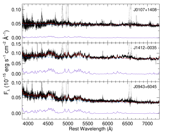
Figure 1: Upper panel. Emission line-subtracted spectrum of J0107+1408. Emission lines are shown with dotted lines, the total continuum fit is shown in red, including the combined reddened power laws as the dashed blue line, and the reddened Fe II component is shown in purple. Middle panel. Continuum fit of J1412–0035 with the same convention as above. Lower panel. Continuum fit of J0943+6045 with same conventions as above.

Our investigation is focused on the properties of the nuclear gas itself, specifically the emission-line ratios, inferred gas kinematics, and gas-phase metallicities of the objects at the low end of the BH mass distribution. To this end, we want accurate measurements of the emission-line fluxes and shapes, for which we must remove the underlying continuum. At the low nuclear luminosities of most of our sample, starlight from the galaxy becomes a significant contributor to the overall continuum, and could bias the emission-line fluxes if not properly accounted for. In addition to the underlying galaxy, a complete model of the AGN continuum includes a nonstellar power law, typically well-fit by the form $f_{\lambda}\propto\lambda^{\alpha}$ (Richards et al., 2003). The optical spectrum also contains emission from numerous broad Fe II transitions that form a pseudo-continuum underlying many other emission lines of interest (see Figure 1). Because the components of our fits are coupled, our fitting process iterates between continuum and emission line fits, as described below.

For computational simplicity, we divide the sample into two classes of objects – those where the AGN dominates the continuum and the galaxy is not generally measurable, and those where the galaxy contributes a significant fraction of the continuum (see Figures 1 and 2). We treat the fitting of these AGN-dominated and galaxy-dominated spectra separately because there are strong degeneracies between the power-law shape, the galaxy continuum level, and extinction. We use the IRAF routine splot to measure the equivalent width (EW) of the Ca II K $\lambda 3933$ Å absorption feature in a user-defined window. We then determine an empirical division between AGN-dominated and galaxy-dominated objects based on this EW. After inspection of the spectra and comparison to the measured Ca II EWs, we determine that galaxy-dominated objects typically have Ca II K EW $>1$ Å, and therefore all such objects are fitted using our galaxy-dominated procedure. For both AGN-dominated and galaxy-dominated fitting methods, we start with an initial continuum fit, then iterate between emission line fitting and continuum fitting, analogous to the procedure to remove Fe II in Netzer & Trakhtenbrot (2007). After three iterations, the H$\alpha$ flux changed by $<0.001$% for the median objects, but there were two objects where the changes were at the 10% level at the final iteration. Still, this 10% change is within our final errors as described below. The ratio of H$\beta$ fluxes between iterations also typically converged to within 0.001% of the final value, but was up to 1% for two objects.

3.2 Continuum Fits

For AGN-dominated objects, the continuum fitting windows included the following regions: 3900–4330, 4430–4770, 5020–5650, and 7600–7900 Å. Examples of our AGN-dominated objects are shown in Figure 1. For these objects, we applied a continuum fit that included two power laws, Fe II pseudo-continuum, and reddening. There are many degeneracies in these fits between internal extinction, Galactic extinction, flux calibration errors, and the intrinsic shapes of the AGN and galaxy continua. Barth et al. (2005) and Xiao et al. (2011) use a quadratic polynomial in addition to a power-law and galaxy continuum to account for the additional terms. We have chosen to include a single reddening law instead. We adopt the reddening prescription in Calzetti et al. (2000) for star-forming galaxies, since our objects have blue, disky host galaxies (Greene et al., 2008). Note that by using the Calzetti et al. reddening law we have implicitly assumed a dust opacity and geometry that may not be applicable to these AGN. Our original hope was to glean additional physically meaningful information from the fits including extinction. After comparing the Balmer decrements with the continuum-derived reddening, we determined that due to the degeneracies described above, our continuum-derived extinction terms are not robust. Therefore, we use the extinction term only to derive satisfactory continuum fits.

Although our spectral region only includes 3800–8500 Å, we find that two power laws are needed in 38% of the AGN-dominated objects, where the power laws are defined as $f_{\lambda}\propto\lambda^{\alpha}$. AGN often show a break in the slope of the continuum around 5000 Å, with the blue region steeper than the red, which is commonly fitted with a broken power law (Shang et al., 2005). This upturn in the blue end of the continuum is not due to the accretion disk emission known as the little blue bump (Shields, 1978), which ends around 4000 Å, but represents a real break in the power law continuum. We cannot tell if this break is due to increasing galaxy continuum toward the red (Vanden Berk et al., 2001), because there are not enough stellar features to accurately model the galaxy in these AGN-dominated objects. Initial parameters for the power laws are based on the H$\alpha$-$L_{5100}$ relation described in Greene & Ho (2005b). The power-law slopes were free to vary, but were both limited to have indices less than or equal to zero (median index $\alpha=-1.30$) in order to reduce degeneracy with extinction. For all fits requiring a broken power law, one of the fitted power laws is flat with an index of zero, which dominates the red end of the spectrum, and the other power law dominates the blue end with an average power-law index of $\alpha=-2.26$. We note again that there is still some degeneracy between the blue power-law slope and the level of extinction.

We fitted the Fe II pseudo-continuum by scaling, broadening, and shifting the empirical model from Boroson (2002), which is based on the prototypical strong Fe II object I Zw 1. Fitting empirical templates from I Zw 1 is a well-established method for dealing with the Fe II in optical and UV spectra (e.g., Boroson & Green, 1992; Vestergaard & Wilkes, 2001; Boroson, 2002; Leighly & Moore, 2006). For typical AGN, the I Zw 1 template fits the Fe II pseudo-continuum well (Kovačević et al., 2010). While templates have been made using theoretical Fe II atomic models (Verner, 2000), these are limited by the the complexity of the Fe II ion and the lack of laboratory data on the atomic transitions. We should note that the structure within the Fe II pseudo-continuum differs from the structure of the I Zw 1 template in several of our galaxies, as seen by Kovačević et al. (2010) and Hu et al. (2008b).

For the galaxy-dominated spectra, we applied a continuum fit over the following wavelength regions to include more stellar absorption lines than the pure AGN fits: 3900–4300, 5020–5650, 5870–5920, 6150–6530, and 7100–7700 Å. Our galaxy-dominated fits included a single power law, a model galaxy spectrum with an age of 10 Gyr, and reddening. The power-law index for these objects was fixed at $\alpha=-1.56$ as in Vanden Berk et al. (2001) with a starting amplitude based on the H${\alpha}$-$L_{5100}$ relation (Greene & Ho, 2005b). This is somewhat steeper than the median index we find for our AGN-dominated objects ($\alpha=-1.30$). The galaxy model was made using a Bruzual & Charlot (2003) single stellar population model with an age of 10 Gyr, where we assume a Chabrier (2003) initial mass function, and the metallicity is assumed to be solar. Solar metallicity may be an over-estimate for these galaxies (see Section §4), but because of the small aperture of our observations, and the significant dilution from the AGN continuum, we do not have strong constraints on the stellar population parameters. The galaxy model is dominated by emission from K giants in the optical spectral region. The continuum fits of Barth et al. (2005) and Xiao et al. (2011), which utilize stellar templates rather than single stellar population models, also find continua dominated by K giants. The free parameters of this 10-Gyr galaxy model are a broadening function ($\sigma$), model amplitude, and redshift . Note that the spectral models have an intrinsic dispersion that is larger than the galaxy spectra, and thus the fitted $\sigma$ is not physically meaningful. As above, the galaxy and power law components were multiplied by a reddening function, for which we varied $A_{\mathrm{V}}$.

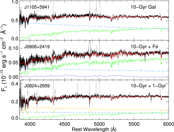
Figure 2: Upper panel. Emission line-subtracted spectrum of J1105+5941. Emission lines are shown with dotted lines, the total continuum fit shown in red, including the reddened power law as the dashed blue line, and the reddened 10-Gyr galaxy component in green. Middle panel. Spectrum of J0806+2419 with the same convention as above, where the additional reddened Fe II component is shown in purple. Lower panel. Spectrum of J0824+2959 with same conventions as above, where the additional reddened 1-Gyr galaxy model is shown in yellow.

For three of our galaxy-dominated objects, including J1240–0029, J2156+1103, J0806+2419, individual inspection revealed Fe II pseudo-continuum in the spectra, so we fitted them with the previous galaxy continuum method, but included the Fe II pseudo-continuum component as well. For four other galaxy-dominated objects (J0824+2959, J1057+4825, J1143+5500, and J1631+2437) an obvious A star-like component was necessary in the 3800–4200 Å region to account for Balmer absorption. For these objects, we included an additional galaxy model component, much like the 10-Gyr model, but with an age of 1 Gyr. We do not find any evidence of systematic differences in host galaxy morphology (Jiang et al., 2011) or line ratios for objects requiring a 1-Gyr galaxy model. Examples of each fitting procedure are shown in Figure 2.

3.3 Emission Line Fits

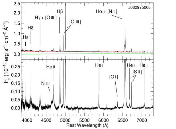
Figure 3: Upper panel. Original spectrum of J0829+5006 with total continuum fit shown in red, including a single power law as the dashed-blue line, and 10-Gyr galaxy continuum in green, which have been multiplied by a reddening law. Lower panel. Zoom in of continuum-subtracted spectrum to enhance the view of weaker emission lines. All fitted emission lines are labeled.

Once the continuum fitting is complete, we have line-only spectra to fit. The emission line-fitting procedure was the same across all continuum types. We fit narrow and broad components to the Balmer lines, from H${\alpha}$ to H${\epsilon}$, narrow and broad He I lines $\lambda$5876, $\lambda$6678, and $\lambda$7065, the [S II] $\lambda\lambda$6717, 6730 doublet, the [N II] $\lambda\lambda$6548, 6584 doublet, [O I] lines $\lambda$6300 and $\lambda$6364, [O III] lines $\lambda\lambda$5007, 4959 and $\lambda$4363, narrow and broad He II $\lambda$4686, and N III $\lambda$4640. The fitted emission lines are illustrated in Figure 3 and are summarized in Table 2, where we list the line species, rest wavelengths, and the components used in the fit. We present derived quantities of our low-mass AGNs in Table 3, and the emission-line measurements for all of our objects in Tables 4 and 5. Note that the fluxes presented have only been corrected for Galactic reddening. Widths of multi-component lines are calculated by constructing the total fit of the line and measuring the FWHM of this reconstruction.

For each object, we fit the NLR emission lines using sets of Gauss-Hermite functions, much like Salviander et al. (2007). The expression for a set of Gauss-Hermite functions is as follows:

$$F(x)=Ae^{-x^{2}/2}[1+h_{3}f_{3}(x)+h_{4}f_{4}(x)]\\$$ (1)

$$f_{3}(x)=\frac{1}{\sqrt{6}}(2\sqrt{2}x^{3}-3\sqrt{2}x)\\$$ (2)

$$f_{4}(x)=\frac{1}{\sqrt{24}}(4x^{4}-12x^{2}+3)\\$$ (3)

where

$$x=(\lambda-\lambda_{\mathrm{cent}})/\sigma.$$ (4)

When using a single set of Gauss-Hermite functions, each emission line is fit with five parameters: line centroid, width ($\sigma$), flux, $h_{3}$, and $h_{4}$. The $h_{3}$ parameter quantifies the asymmetry of the line and $h_{4}$ measures the kurtosis, or boxiness, of the line. Therefore, we can in principle quantitatively compare NLR line shapes among objects. This works well for NLR emission with the exception of [O III], where 74% of our objects are not well-described by a single set of Gauss-Hermite functions, as described below. In general, we base the NLR line shapes on a fit to the [S II] doublet because it is in a relatively clean region of the spectrum, is not blended with other lines, and is usually strong enough to constrain the line shape (e.g. Ho et al., 1997b; Greene & Ho, 2004). Unless otherwise noted, all NLR lines are fixed to have the same velocity width, $h_{3}$, and $h_{4}$ as the [S II] fit. The wavelengths for each species are fixed to their relative laboratory ratios. The flux ratio of the [N II] doublet is fixed to its laboratory value of 2.96. We also fix the [O III] $\lambda$4363 line to have the same shape and number of components as the [O III] $\lambda$5007 fit, such that its flux is the only free parameter. In two cases, J0806+2419 and 1534+0408, the narrow H$\beta$ line was so weak that we imposed a limit that H$\beta$ could not exceed H$\alpha_{\mathrm{NLR}}/3$.

For the [O III] $\lambda$5007 line, we try an initial fit with one Gauss-Hermite function for each line, with starting values taken from the [S II] fit, but all five parameters free. As described above, [O III] lines are often complex in AGN and can have strong wavelength shifts and/or asymmetries, so we allow the code to fit the lines with two summed Gauss-Hermite functions, and again allow the code to determine if there is a statistically significant improvement with the additional component. We find that 74% of our spectra require two components for the [O III] fit, and of those, 85% had a blueshifted second component.

While we tried fitting the BLR lines with Gauss-Hermite functions as well, we found that more than one Gauss-Hermite component is required to model the broad lines. This is in contrast with Salviander et al. (2007), where they were able to model H$\alpha$ and H$\beta$ with single sets of Gauss-Hermite functions. Our observations have much higher resolution and S/N than the SDSS spectra they used, and thus we have robust measurements of two component BLRs. Therefore, we chose to fit the broad lines with sums of Gaussians, because the interpretation of summed Gauss-Hermite functions becomes no more intuitive than sums of Gaussians, and in fact, has more degeneracies among the fit parameters.

For the broad H$\alpha$, we allow the code the freedom to use up to four Gaussians and to pick the most effective fit for the number of free parameters included. Using a criterion inspired by Hao et al. (2005), the code determines the benefits of adding each additional Gaussian to the fit by comparing the number of additional model parameters to the improvement in $\chi^{2}$. We apply this same procedure to the broad H$\beta$, with up to three possible summed Gaussians. Examples of our H$\alpha$ and H$\beta$ fits are shown in Figure 4. We then subtract the fit of the H$\alpha$ complex from the line spectrum, in order to fit the He I lines.

3.4 Error Analysis

To estimate uncertainties on our emission line fits, we generate Monte Carlo simulations of each galaxy spectrum. To construct the model, we take the measured values from the final continuum and emission line fits and reconstruct the spectrum, to which we add Gaussian random noise using the measured error array. For each object, we construct 100 such fake spectra and fit them using our continuum and emission line fitting prescription. The final uncertainty is defined by the distribution of measurements of the artificial spectra. Specifically, we use the width encapsulating 68% of the results.

Of course, we also incur systematic errors in our continuum fitting. To estimate their magnitude, we explore the consequences of removing components from the most complicated fits: those requiring a young (1-Gyr old) galaxy component. We explore fits without the 1-Gyr continuum component and with or without an FeII pseudocontinuum component. Even in this rather extreme case, the flux ratio of the narrow H$\alpha$/H$\beta$ lines typically only varies by 10% or less across all the different fits, although one object showed a factor of two increase with the addition of the 1-Gyr galaxy component.

We also compare our fitted measurements of the narrow and broad components of H$\alpha$ to those made by Xiao et al. (2011) on many of the same objects, and find that 93% of our measured widths are consistent to within 1$\sigma$ and 75% have fluxes consistent to within 20% of the measured value. This provides a valuable additional measure of systematic errors and is consistent with our measured uncertainties.

4 Gas-Phase Metallicity

Because AGN are some of the most distant observable objects, metallicities in AGN are used as a possible tracer of the history of chemical evolution in the universe (Hamann & Ferland, 1999). While investigation of high-redshift AGN typically probes the BLR metallicity, here we focus entirely on the metallicity of the NLR, which should be more representative of the gas-phase metallicity of the central region of the galaxy. AGN typically have super-solar metallicities, as measured with diagnostic emission lines in the NLR. Groves et al. (2006) found that out of a sample of $\sim 23,000$ AGN from SDSS, only 40 showed sub-solar metallicities. To some degree, this result is biased by the difficulty of finding low-mass BHs in late-type, star-forming galaxies with sub-solar gas-phase metallicities. Only a handful of low-metallicity, dwarf galaxies which harbor AGN have been detected to date (Kraemer et al., 1999; Izotov & Thuan, 2008). Thus, we still do not know how intrinsically rare these low-mass BHs are (e.g. Greene & Ho, 2007a). We suspect that when AGN are found in low-mass galaxies, the gas-phase metallicities will be low and in accord with the mass-metallicity relation of inactive galaxies (e.g. Tremonti et al., 2004). We test that supposition directly here using the NLR emission lines.

We investigate the gas-phase metallicities of the objects in our low-mass, low-luminosity sample using several rest-frame optical NLR emission-line diagnostics. Because nitrogen is a secondary element, as the abundances of metals relative to hydrogen increase, the abundance of nitrogen relative to other metals also increases. As a result, the ratio of nitrogen to hydrogen is a good metallicity diagnostic, and in particular, [N II]$/$H$\alpha$ has traditionally been used in research on AGN and other nebulae (Pagel & Edmunds, 1981; Evans, 1986). The locus of low-metallicity objects is easily seen in the well-known Baldwin, Phillips, Terlevich (BPT) diagram (Baldwin et al., 1981). For a given [O III]$/$H$\beta$, AGN that have a lower [N II]$/$H$\alpha$ are likely at lower relative metallicity.

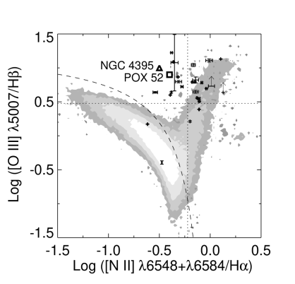
Figure 5: BPT diagram of SDSS DR7 galaxy sample in grayscale contours, and our low-mass AGN as crosses, with low-mass AGN NGC 4395 and POX 52 for comparison. Also plotted is the theoretical Kauffmann et al. (2003) divider (dashed) between starburst galaxies (below) and AGN (above), and the dotted Ho et al. (1997a) lines, which separate Seyferts (upper right) from LINERs (lower right).

For the sake of comparison to typical AGN, we compare our sample of low-mass AGN with a subset of the SDSS DR7 galaxy sample at $z\approx 0.1$. Spectral measurements for the SDSS subset have been taken from the catalog compiled by the Max-Planck-Institute for Astrophysics/Johns Hopkins University (MPA/JHU) group. The fitting process used to construct the catalog is described in Brinchmann et al. (2004) and Tremonti et al. (2004). Note that the catalog selects narrow-line AGN. We select only objects whose H$\alpha$, H$\beta$, [O III], and [N II] emission lines had errors $<10\%$ of the flux of the lines, which results in a total of 147,816 objects, plotted in grayscale in Figure 5. Star-forming galaxies lie to the left of the dotted line at log [N II]$/$H$\alpha<-0.2$, and AGN are in the plume extending to the upper right. Two of our galaxies, J1143+5500 and J2156+1103, fall into the star-forming region as denoted by the Kauffman et al. dashed line, indicating contamination from H II regions within the host galaxies. While the presence of broad emission lines in our objects confirms the presence of an AGN in these two galaxies, they must have substantial contributions from star formation within the host galaxy. Compared to local AGN in DR7, our sample of low-mass AGN extend to lower [N II]$/$H$\alpha$ than the SDSS AGN, which seems to indicate that the low-mass AGN include objects at relatively lower metallicities than the bulk of SDSS AGN. Husemann et al. (2011) also see this trend with the large sample of low-mass SDSS AGN presented in Greene & Ho (2007a).

We want to determine absolute metallicities for our low-mass AGN to confirm whether they do represent the apparently rare, sub-solar AGN. However, it is difficult to define metallicities for AGN on an absolute scale. Dopita et al. (2002) and Groves et al. (2004a) have developed photoionization models that include the photoionization structure and emission from dusty, radiation pressure-dominated gas. To this end, they employ MAPPINGS III, a photoionization and shock code whose development is detailed in Dopita et al. (1982) and Sutherland & Dopita (1993). MAPPINGS III considers patches of gas to have the whole range of ionization structure, thereby producing emission which contributes to virtually all of the lines observed in an NLR. Dopita et al. (2002) argue that by causing the radiation pressure to dominate the pressure gradient of the gas, their models can predict emission line ratios that are consistent with the observed values seen in real systems (Groves et al., 2004b). Note that MAPPINGS III reports a total metallicity, not a gas-phase metallicity, so the MAPPINGS III metallicities may be systematically higher than other literature values. For a more extensive overview of photoionization modeling methods, see also Groves (2007).

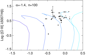
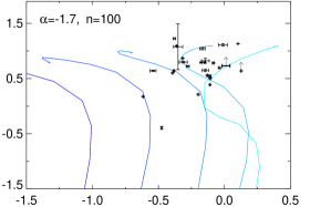
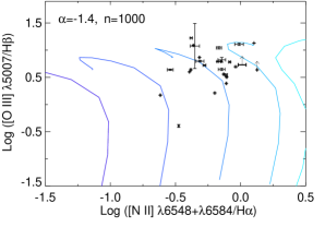
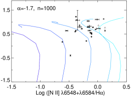
Figure 6: MAPPINGS III models used to determine the metallicities in our sample, where $Z=0.25,0.5,1,2,$ and $4~{}{Z}_{\odot}$, from left to right, and log $U$ ranges from $-4$ to $0$ from bottom to top (Top row: n$=100$ cm^-3, Bottom row: n$=1000~{}$cm^-3, Left column: $\alpha=-1.4$, Right column: $\alpha=-1.7$). Using these grids, our sample shows a range of metallicity estimates, with most objects having super-solar metallicities.

We estimate metallicities in our objects by comparing the [O III]$/$H$\beta$ vs. [N II]$/$H$\alpha$ measurements for our sample of AGN to the predictions from the MAPPINGS III grid of models. For our sample, we are able to estimate the density in the NLR using the [S II] doublet ($100\lesssim n_{e}\lesssim 1300$, see Table 3) and to constrain the shape of the AGN continuum based on previous observations of $\alpha$ for AGN ($\alpha=-1.56$; Vanden Berk et al. 2001). This allows us to utilize models that are appropriate for our particular sample. These dusty, radiation pressure-dominated models are publicly available within the library of grids provided in the IDL code ITERA (Groves & Allen, 2010). In Figure 6, we show our low-mass AGN measurements compared to four grids of models, which represent the full variety of physical parameters we see in our objects, including $n_{e}=100$ cm^-3 and $1000~{}$cm^-3, and $\alpha=-1.4$ and $-1.7$. While there are some regions of the grids that can be described by several models, especially at high log $U$ and steep indices ($\alpha=-1.7$), generally the metallicity increases with increasing [N II]$/$H$\alpha$. The metallicity estimates derived from the MAPPINGS III code can vary by up to a factor of three in metallicity, depending on the range of $\alpha$ considered. MAPPINGS III metallicity estimates for individual objects can range from sub-solar to several times solar depending on the assumed spectral shape. Our metallicity estimates are presented in Table 3. There are also several objects that lie at the upper edge of the models, which may reflect limitations of the models.

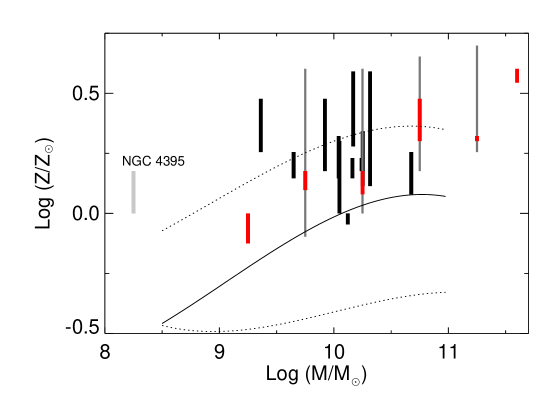
Figure 7: Host galaxy stellar mass vs. NLR metallicities for our sample (Fig. 6) as solid black bars. The range in $Z$ represents the effect of a reasonable range in assumed ionizing slope in the modeling. Solid red bars are obscured AGN from the SDSS DR7 with metallicities derived in the same way. The 1$\sigma$ variation over each mass bin is shown in grey. The solid curve represents the Kewley & Ellison (2008) stellar mass-metallicity relation based on [O III] and [N II], which is bracketed by dotted lines showing the most extreme relations they present (KK04 is uppermost and P05 is lowermost).

To do a relative comparison, we investigate trends between our low-mass AGN and the SDSS sample of AGN using the MAPPINGS III models. To derive the metallicity for each of our galaxies, we consider where an object lies on a particular MAPPINGS III grid, and interpolate between the two nearest metallicity tracks to determine a metallicity ($Z$) for that object (see Figure 6). For each object, we estimate the metallicity from grids with the nearest density, $n_{e}=100$ cm^-3 or $n_{e}=1000$ cm^-3. The average change in metallicity between models with $n_{e}=100$ cm^-3 and $n_{e}=1000$ cm^-3 at fixed $\alpha=-1.4$ is only $0.02~{}{Z}_{\odot}$, so density differences are negligible. However, the difference in metallicity for $\alpha=-1.4$ versus $\alpha=-1.7$ is $0.3~{}{Z}_{\odot}$, and since the errors in our slopes are large, we incorporate this uncertainty into our results. We estimate the metallicity using both $\alpha=-1.4$ and $\alpha=-1.7$, but exclude estimates for the $\alpha=-1.7$, $Z=4~{}{Z}_{\odot}$ model, because it is degenerate with the other models in the region of interest (see Figure 6). This gives a range of $Z$ for each object presented as black bars on Figure 7.

To highlight the difficulties in deriving absolute metallicities, we consider the particular case of NGC 4395, a well-studied, low-mass AGN. We have an ESI spectrum of NGC 4395, for which extensive measurements and Cloudy modeling are published (Kraemer et al., 1999), and we find that our observed emission- line ratios agree with the previous measurements [log ([N II]$/$H$\alpha)~{}\sim~{}-0.5$, log ([O III]$/$H$\beta)~{}\sim~{}1.0$]. Kraemer et al. (1999) estimate a metallicity of $Z\sim~{}$0.25 ${Z}_{\odot}$, which is consistent with estimates made from the H II regions. Since then, the definition of solar metallicity has been revised because of new oxygen measurements (Asplund et al., 2004), such that solar metallicity is now defined to be a factor of two lower than previously thought. Therefore the estimate of metallicity from Kraemer et al. (1999) actually supports a metallicity for NGC 4395 of 0.5 ${Z}_{\odot}$. To estimate a metallicity from the MAPPINGS III grids, we need to determine the density and power-law index for NGC 4395. Using the [S II] $\lambda 6717,6731$ doublet, we estimate that the density in the NLR of NGC 4395 is about 1300 cm^-3, and Kraemer et al. (1999) also constrains $\alpha_{\mathrm{o}x}\sim-1.7$ for NGC 4395. Using these values, we estimate the metallicity of NGC 4395 to be $Z\sim 1.5~{}{Z}_{\odot}$ from the MAPPINGS III models that have n$=1000~{}$cm^-3and $\alpha=-1.7$ (Figure 6). There is a significant zero-point offset between the two sets of photoionization models, as has been well described in other contexts. Again, we note that the absolute scale of the gas-phase metallicities remain highly uncertain. For instance, one reason the MAPPINGS III values appear high is that the depleted metals are counted (i.e., we calculate the total, rather than gas-phase metallicity). Other factors, such as the photoionization modeling methodology, are likely at play as well. In the following, we use metallicity estimates from the MAPPINGS III models so that we can compare directly with Groves et al. (2006), but focus only on relative trends between objects rather than absolute metallicities. Our approach is analogous to that advocated by Kewley & Ellison (2008) for star-forming galaxies.

For comparison to AGN with more massive BHs, we selected AGN from the SDSS DR7 galaxy sample described above using the cuts from Ho et al. (1997a) for Seyferts ([S II]$/$H$\alpha>0.4$ and [O III]$/$H$\beta>3$). This results in 3747 galaxies, which are binned according to the stellar mass reported by the MPA/JHU group in increments of 0.5 dex between $9.0<~{}$log $M_{*}/{M}_{\odot}<12.0$. For each stellar mass bin, we estimate $Z/{Z}_{\odot}$ from the MAPPINGS III grids using the median [N II]/H$\alpha$ and [O III]/H$\beta$ value for that bin (red bars in Figure 7 denote the range of metallicities that result from the range of $\alpha$ as above). We also estimate the range of $Z$ for the central 1$\sigma$ of the objects in each bin in the same way (grey bars in Figure 7), except for the highest- and lowest-mass bins which had fewer than 40 objects. Because these SDSS AGN cover the same range of densities as our low-mass AGN (300-1500 cm^-3), we estimate their $Z$ from the same MAPPINGS III grids as described above.

We present our relative metallicity comparison in the context of the $M_{*}$-$Z$ relation in Figure 7. The $M_{*}$-$Z$ relation is only defined for star-forming galaxies and has never been measured in AGN host galaxies before to our knowledge. For several of our low-mass AGN, we derive a stellar mass from the Hubble Space Telescope (Greene et al., 2008) I-band luminosities and a mass-to-light ratio based on the SDSS g-r color following Bell et al. (2003). These stellar masses and our metallicity estimates are presented in Table 3. To expand the low-mass end of the sample, we include NGC 4395 for comparison, with metallicities estimated from the MAPPINGS III grids. We also plot the Kewley & Ellison (2008) $M_{*}$-$Z$ relation for star-forming galaxies that is based on [O III] and [N II] (referred to as PP04 O3N2), which is the closest analog to our method but was derived for a star-forming spectral energy distribution. For those low-mass AGN with $10.0<$ log $M_{*}/{M}_{\odot}\leq 10.5$, which includes most of our objects, we find that the mean $\langle Z/{Z}_{\odot}\rangle=0.11$, which is somewhat higher than the $Z$ predicted by the $M_{*}$-$Z$ relation for star-forming galaxies shown by the solid curve. In comparison, the metallicities of our objects agree with the SDSS AGNs at the same mass.

Even without modeling, our low-mass AGN include objects that have a lower ratio of [N II]$/$H$\alpha$ relative to the SDSS AGN (Figure 5), which suggests lower metallicities. This confirms our suspicion that since our host galaxies extend to lower mass than the SDSS galaxies, the low-mass AGN include lower-$Z$ objects. There appears to be a systematic difference between the active and inactive galaxies, in the sense that the active ones appear to have higher average metallicities at fixed stellar mass (Figure 7). Either we are seeing systematic differences due to methodology (i.e. different ionizing spectra) or it is a real effect. Since the NLR is compact compared to the interstellar medium of the galaxy as a whole at these luminosities (e.g. Schmitt et al., 2003), we are probing the high-metallicity central region of the galaxy. Given well-known metallicity gradients in spiral galaxies (e.g. Henry & Worthey, 1999), we may be slightly overestimating the overall gas-phase metallicity in the active galaxies.

Our investigation shows that determining absolute metallicities for AGN is a very complex problem, and as suggested in other contexts, we can only trust relative metallicity information derived using the same methodology across samples. While the AGN in our sample have similar NLR metallicities as the SDSS AGN at fixed stellar mass, our low-mass AGN include objects at somewhat lower metallicities than SDSS AGN, at least in part because they occupy lower-mass host galaxies. We estimate metallicities using [N II]$/$H$\alpha$ and photoionization models. Barth et al. (2008) present the Seyfert 2 counterparts to our low-mass Type 1 AGN, which have overlapping [N II]$/$H$\alpha$ and [O III]$/$H$\beta$ values and therefore similarly likely include low-$Z$ objects as well. Because of the uncertainties from the models we cannot say for sure whether our objects are the rare, sub-solar metallicity objects addressed by Groves et al. (2006). Conversely, when directly compared to the metallicity predictions from the $M_{*}$-$Z$ relation for star-forming galaxies, AGN are consistent with obeying a comparable mass-metallicity relation as inactive galaxies, although the scatter is large.

4.1 Metallicity Systematics

As we will see in §5, there is tentative evidence for a steeper far-UV continuum slope in these systems of $\alpha=-2.0$. If we assume a steeper slope of $\alpha=-2.0$ for the photoionization models, this would only minimally impact the metallicity estimate of objects with estimates $Z<1~{}{Z}_{\odot}$, causing $Z$ to increase by $\sim 0.2$. A steeper slope of $\alpha=-2.0$ could potentially increase the measured metallicities by up to a factor of two for objects with $Z>1~{}{Z}_{\odot}$, but this does not change our previous conclusions that some of these low-mass AGN potentially represent the rare, low-metallicity AGN sought in Groves et al. (2006).

Line emission from star formation in the host galaxy could also potentially affect our metallicity estimates. To estimate the magnitude of the changes, we take two representative AGN with metallicities of solar and twice solar. We then add varying levels of star formation, assuming gas at the same metallicity and deriving the appropriate line ratios from Pettini & Pagel (2004). For instance, an AGN with a solar gas phase metallicity will have [O III]/H$\beta\approx 6$, while the star forming regions will have [O III]/H$\beta\approx 0.2$. In the extreme case that 75% of the Balmer emission comes from star formation, the observed line ratio would be [O III]/H$\beta=1.7$. For solar metallicity, we underestimate the metallicity estimates only by 10–30% for a 25–75% contribution from star formation to the Balmer line flux. At twice solar, 50–75% contribution from star formation leads to a factor of 2–3 underestimate in metallicity. However, only two sources, J1143+5500 and J2156+1103, lie far enough from the AGN locus to be consistent with this level of contamination (Fig. 5). Thus, we conclude that contributions from star formation do not change our metallicity distribution significantly.

5 Spectral Energy Distribution

In theory, the lower masses of these BHs should correspond to a hotter accretion disk temperature and thus measurable differences in the spectral energy distributions (SEDs) of our sample from those of more typical AGN. Testing this expectation will help to bridge the gap in BH behavior and accretion theory from stellar mass BHs to the largest SMBHs. In addition, the nature of the accretion disk surrounding these low-mass AGN can inform our understanding of the primordial intermediate-mass BHs that formed within the first galaxies and participated in the reionization of the Universe (Milosavljević et al., 2009). We know that the SEDs of accretion disks around stellar mass BHs are harder and flatter than those of quasars (Frank et al., 2002). In fact, the peak blackbody temperature for disks in AGN with low-mass BHs may also move into the X-ray band (Done et al., 2012). We have seen hints of SED changes in this sample in previous work, both in $\alpha_{\mathrm{o}x}$ (Desroches et al., 2009) and in EW_Hβ (Croom et al., 2002; Greene & Ho, 2005b). While most of our objects have been studied at radio (Greene et al., 2006) and X-ray (Greene & Ho, 2007b; Desroches et al., 2009; Miniutti et al., 2009) wavelengths, we have no direct constraints on the far-UV continuum. We can gain an indirect handle on the accretion disk shape, however, since those photons are responsible for photoionizing the emission line gas that we observe in the optical.

Specifically, we can infer the slope of the continuum in the far UV by contrasting the He II and narrow H$\beta$ components. As described in Penston & Fosbury (1978), since both H$\beta$ and He II are recombination lines, the ratio of their relative strengths should yield a measure of the relative intensity of the continuum at 912 Å and 228 Å, the ionization edge for He II. Assuming the ionizing source is well-described by a power law of the form $I_{\nu}\propto\nu^{\alpha_{\rm UV}}$, the intensities should behave as follows:

$$\frac{I_{4686}}{I_{H\beta}}=1.99\times 4^{\alpha_{\rm UV}}$$ (5)

As the BH mass decreases at fixed Eddington ratio, we would expect to move closer to the peak of the big blue bump, and thus to observe shallower $\alpha_{\rm UV}$ as a function of mass. Of course, many other factors may be at play, including differing Eddington ratio distributions or different reddening (e.g. Bonning et al., 2007). The deduced UV power-law slopes for our objects range from $-4<\alpha_{\rm UV}<-0.4$, with a median value of $-1.9$. To compare to a sample of typical AGN, we consider the low-redshift AGN presented by Ho & Kim (2009), which have $M_{\mathrm{BH}}\sim 10^{6}-10^{8}~{}M_{\odot}$ and a median absolute magnitude of $M_{B}\sim-19$ derived from their H$\beta$ luminosities. Because their observations were taken on the Magellan 6.5 m Clay Telescope, they have data of similar quality to ours. They measured many emission lines, including He II and H$\beta$. We use their measured line ratios to calculate $\alpha_{\rm UV}$ for their 94 objects, and present the distribution of the two samples in Figure 8. The comparison sample has a range from $-2.5<\alpha_{\rm UV}<0.3$, with a median slope of $-1.4$. A KS test of the two distributions results in $P<0.001$, meaning that there is less than 0.1% probability that they are drawn from the same parent sample. We find that the distributions are statistically different whether we include the three low-mass AGN with upper limits in our distribution or not.

Given this difference in distributions, and the significant shift in the median, we also look for a correlation between $M_{\mathrm{BH}}$ and $\alpha_{\rm UV}$. We find a mild correlation, with a correlation coefficient $r=0.18$ for the range of BH masses included here, from $5.5<$ log $M_{\mathrm{BH}}/{M}_{\odot}<10$. A least-squares fit to the data yields the following relationship: log $M_{\mathrm{BH}}\propto 0.10~{}\alpha_{\rm UV}$. Previous work (Shang et al., 2005; Davis et al., 2007) investigate possible correlations between the UV continuum slope and $M_{\mathrm{BH}}$ and do not find compelling evidence for a trend between UV slope and $M_{\mathrm{BH}}$. We probe a bluer region of the UV continuum and extend to lower $M_{\mathrm{BH}}$ than those authors, and we see a tantalizing hint for a correlation between $M_{\mathrm{BH}}$ and $\alpha_{\rm UV}$. On the other hand, the sense of the trend is counter to our naive expectations for lower-mass BHs. It would be useful to compile a sample including our low-mass BHs with matched Eddington ratios and examine both the X-ray and UV spectral slopes at the same time (e.g. Desroches et al., 2009).

6 Composite Spectra

An effective way to highlight general spectral characteristics is to make composite spectra. Other authors in AGN research have used composite spectra to investigate trends in AGN across a wide range of redshifts (Vanden Berk et al., 2001), to probe weak emission lines in high luminosity AGN (Francis et al., 1991), and weak emission and absorption lines in $z=2-3$ star-forming galaxies that house AGN (Hainline et al., 2011). One advantage of a composite spectrum with our high spectral resolution is that it gives us the opportunity to investigate low-contrast features that would otherwise be difficult to detect, including faint emission lines, line wings, and intermediate-line regions. Some of our objects exhibit high-ionization, forbidden Fe lines, such as [Fe VII] $\lambda 6087$, [Fe X] $\lambda 6374$, and [Fe XI] $\lambda 7892$. These coronal lines are thought to originate in the inner edge of the NLR, where densities are low enough to allow forbidden line emission, but the ionization parameter is high enough to enable ions like Fe⁺⁹ to exist. Mullaney et al. (2009) compare the line shapes and shifts of the centroid of these lines to [O III]. They find that the high-ionization lines are at similar offsets, and therefore similar velocities, to the blue wing of [O III], which may originate in outflowing material (De Robertis & Osterbrock, 1984; Cecil et al., 2002; Gelbord et al., 2009). With the luxury of very high spectral resolution and S/N, we can both investigate the trends highlighted in previous works in more detail and determine whether they hold for these low-mass, low-luminosity systems.

6.1 Composite of Entire Sample

We construct our composite spectra by interpolating all the spectra to the same rest-wavelength grid using [S II], normalizing them to the rest-frame AGN continuum at 5600 Å, and then taking the median flux value of contributing objects at each wavelength. This method is similar to the median composite construction presented in Vanden Berk et al. (2001). To highlight the weak features, we construct our composites from the continuum-subtracted spectra. In Figure 9, we present the composite spectrum of the original spectra including all 27 low-mass AGN, which highlights the many weak NLR emission that we observe, and in Table 5 we present our measurements of the many NLR emission lines in this composite.

In our continuum-subtracted composite, which highlights emission line features, we first investigate broad H$\alpha$ and H$\beta$, to compare the BLRs in our low-mass AGN to those of more massive AGN. Greene & Ho (2005b) investigate the relationship between the FWHM of H$\alpha$ and H$\beta$ for a sample of over 200 AGN from the SDSS, which were selected to have high S/N and low galaxy contamination. They find that H$\beta$ is commonly broader than H$\alpha$, and fit a relation between the two. Within our composite spectrum, we also find that the wings of the H$\beta$ line are broader than those of H$\alpha$. This trend can be seen in our individual fits as well, with a median FWHM of H$\alpha$ of 840 km s^-1 and a median FWHM of H$\beta$ of 1195 km s^-1. In the accepted model of the BLR, where the emission lines are primarily broadened by their Keplerian velocities, H$\beta$, being broader, is emitted from gas interior to the region emitting H$\alpha$ (Osterbrock & Ferland, 2006, and references therein).

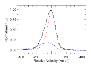
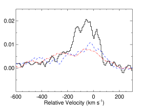
Figure 10: left panel: Line profiles of [O III] in black (solid), [S II] $\lambda 6731$ in red (dashed), and [Fe VII] $\lambda 6087$ in blue (dot-dashed) in velocity space. The line fluxes have been scaled for easier visibility. right panel: Line profiles of [Fe VII] $\lambda 6087$ in black (solid), [Fe X] $\lambda 6375$ in red (dot-dashed), and [Fe XI] $\lambda 7892$ in blue (dashed) in velocity space. In both panels, $v=0$ is with respect to [S II].

Turning to the NLR, we investigate the line shapes of some of the strongest NLR emission lines, including [O III], [S II] $\lambda 6731$, and the high-ionization [Fe VII], to see if the results from Mullaney et al. (2009) hold for AGN of lower mass (see Figure 10). While [S II] and [O III] have very similar profiles on the red side, [O III] shows substantial excess flux on the blue side. It turns out that [Fe VII], much like the profiles in Mullaney et al. (2009), lies mostly under the blue wing of [O III]. The common velocity structure of the blue wing and the high ionization lines supports the idea that the high-ionization Fe lines are emitted in an outflow from the inner face of the dusty torus, and appears to hold true even for our smaller scale low-mass AGN.

We also present multiple high-ionization Fe lines in Figure 10, which all have ionization potential $>~{}100$ eV. In the composite of all 27 low-mass AGN, the [Fe VII] line is blueshifted by $\sim 75$ km s^-1 and the [Fe X] line blueshifted by $\sim 125$ km s^-1 relative to [S II]. The [Fe X] line is also broader than the [Fe VII] line. Unfortunately, the composite shows only a marginal detection in the [Fe XI] line, but the [Fe VII] and [Fe X] lines suggest that as the ionization level of these Fe lines increases, they get broader and more blueshifted. This pattern has been seen in high-ionization, forbidden lines in AGN by many authors (Grandi, 1978; Cooke et al., 1976; Penston et al., 1984). In comparison to Gelbord et al. (2009), who investigate 63 AGN from SDSS which are selected to have high-ionization forbidden lines, the increasing FWHM and blueshift of high-ionization Fe lines in our low-mass AGN most closely resemble their NSL1 and Seyfert 1.5 subsets. Increasing FWHM and blueshift at high ionization potential have also been identified using near-infrared, high-ionization, forbidden lines of various elements, including S, Si, Fe, Ca, and Al, by Rodríguez-Ardila et al. (2011). One would expect this behavior if, as the high-ionization, forbidden lines increase in ionization potential, they are emitted from closer to the nucleus than other NLR lines, and are nearer the launching point of an outflow (Heckman et al., 1981; Ward & Morris, 1984). A possible alternative explanation is that the high-ionization emission results from inflowing material on the far side of the central engine, which is still blueshifted from our point of view; however, the higher ionization lines would still be spatially closer to the nucleus with their stronger blueshifts.

Because the high-ionization Fe lines suggest a possible relationship between ionization potential and line widths and shifts, we investigate several lower-ionization, narrow lines to look for trends with ionization potential, as discussed in Osterbrock & Mathews (1986) and references therein. We fit the composite spectra with our emission-line fitting procedure as described above. In addition, we measure line widths and shifts of weaker lines presented here using a single Gaussian fit to each line in the continuum-subtracted composite spectrum, because there is not enough signal in the high-ionization lines to make a more complicated fit informative. We do this analysis on the composite spectrum rather than individual spectra because the high-ionization lines are weak enough that they are difficult to measure in individual spectra and benefit from the combined signal in the composite. In our individual spectra, only about 20% of our objects have detectable [Fe X] or [Fe XI], despite 16 of 27 showing [Fe VII].

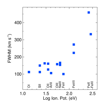
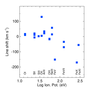
Figure 11: Top: Line widths (FWHM) plotted for NLR forbidden lines from the continuum-subtracted composite of low-mass AGN. Bottom: Line shifts (relative to the centroid predicted from [S II]) for narrow lines from the continuum-subtracted composite of low-mass AGN. Negative shifts are blueward.

In Figures 11 and 11, we show the measured line widths and shifts for a selection of NLR emission lines of varying ionization states in the composite spectrum. In accordance with the trend we see in Figure 10, as the ionization potential of the lines increases, the lines become broader (correlation coefficient of $r=0.88$) and more blueshifted ($r=-0.56$). Again, this is consistent with an ionization structure of the NLR in which the lines with higher ionization potential are emitted closer to the central engine and thus are broader. We postulate that the blueshift indicates an outflowing component on these small scales (Komossa et al., 2008; Müller-Sánchez et al., 2011). Note that nuclear outflows are not typically aligned with the host galaxy in any systematic way. In larger samples, no correlation is seen between the presence of a blue wing and the inclination of the host galaxy (e.g. Greene & Ho, 2005a), and radio jets, which indicate the direction of nuclear outflows, seem to be randomly oriented with respect to their host galaxies (e.g. Kinney et al., 2000). Another commonly discussed correlation is that between FWHM and critical density. We also find a weak trend between critical density and FWHM, as discussed by Filippenko & Halpern (1984) and others. However, with a correlation coefficient of $r=0.54$, this correlation is weaker than that with ionization potential, at least in this sample.

6.2 Division by Physical Properties

While the previous composites are useful for evaluating characteristics of our entire sample, we can also investigate how our spectra change in relation to specific physical or spectral characteristics. To this end, we divide our sample into several subsets. We investigate many characteristics in this manner, including luminosity, Eddington ratio, $M_{\mathrm{BH}}$, FWHM of H$\alpha$, presence or absence of a blue wing in [O III], shift of the centroid of [O III], $h_{3}$ and $h_{4}$ of the NLR fits, and NLR density determined from the [S II] line ratio. In most cases no interesting trends were seen, or they were redundant with those that we show here based on Eddington ratio, luminosity, and the presence of a blue wing in [O III].

For each characteristic, we divide the entire sample of 27 objects into two subsets as described below and construct a continuum-subtracted composite spectrum of that subset. For the luminosity subsets, we derive luminosities from $L_{\mathrm{H}\alpha}$ using the formalism in Greene & Ho (2005b) to calculate $L_{\mathrm{bol}}$. We then divide the sample in half at the median luminosity (log $L_{\mathrm{bol}}=40.5$ erg s^-1, with a full range of $39.3~{}$erg s${}^{-1}~{}<~{}$log $L_{\mathrm{bol}}~{}<~{}41.5$ erg s^-1). To investigate Eddington ratio, we bifurcate the sample about the median Eddington ratio (log $L/L_{\mathrm{Edd}}=-0.4$, with a full range of $-1.8<~{}$log $L/L_{\mathrm{Edd}}~{}<~{}0.3$). To evaluate spectra with or without a blue wing in [O III], we visually inspect the individual continuum-subtracted spectra to determine the presence or absence of a blue wing in [O III] in each object and then form a composite of objects with a blue wing and another composite for those without. Dividing by visual inspection is necessary because of the difficulty of parameterizing blue asymmetry with measurements from the two component [O III] fits. For each of these six composite spectra, we investigate emission line behavior among the NLR emission lines shown in Figure 11. We present the velocity dispersion in the NLR ($\sigma$) for each subset in Table 7, where we subtracted the instrumental resolution ($\sigma_{\mathrm{inst}}=22~{}$km s^-1) in quadrature. These values are averages over all of the NLR emission lines shown in Figure 11 or averages of the high-ionization Fe lines, where the ionization potential $>100$ eV.

Investigation of these subsets yields interesting results for both the BLR and the NLR. We find that the BLR emission lines differ significantly between the high-$L/L_{\mathrm{Edd}}$ and the low-$L/L_{\mathrm{Edd}}$ composites. In Figure 12, we show the H$\alpha$ and H$\beta$ regions for both composites. While the wings of the lines ($v>1200$ km s^-1) are similar, the high-$L/L_{\mathrm{Edd}}$ composite shows excess flux at intermediate velocities in both the broad H$\alpha$ and H$\beta$ emission lines. The difference in intermediate BLR component is unique to the $L/L_{\mathrm{Edd}}$ subset. The intermediate-width component in the high-$L/L_{\mathrm{Edd}}$ composite has a FWHM$=840$ km s^-1, compared to the width of the broad component at FWHM$=2,400$ km s^-1. The intermediate line component is still broader than the average NLR width, shown in Table 6, and also broader than the high-ionization Fe lines. Our discovery of an intermediate line region supports the conclusion of Hu et al. (2008a) that changes in Eddington ratio among objects can account for differences in an intermediate component of the Balmer lines. Increased intermediate-line emission in high-$L/L_{\mathrm{Edd}}$ AGN could bias their derived BH masses, causing underestimates of the true $M_{\mathrm{BH}}$ (Collin et al., 2006; Wang & Wei, 2009).

We also find that NLR emission-line properties are dependent on luminosity, $L/L_{\mathrm{Edd}}$, and the presence of a blue wing in [O III]. When investigating the effects of luminosity, we find that the high-$L_{\mathrm{bol}}$ composite has broader NLR emission lines than both the low-$L_{\mathrm{bol}}$ composite and the general composite of our whole sample. This is in keeping with past findings (Phillips et al., 1983; Whittle, 1985, 1992), where higher luminosities result in broader line widths, commonly thought to be due to the inferred larger gravitational potential of the bulge of the galaxy (Ho et al., 2003). The high-$L/L_{\mathrm{Edd}}$ subset also possesses similarly broad NLR emission lines compared to the low-$L/L_{\mathrm{Edd}}$ subset. Given the small dynamic range in $M_{\mathrm{BH}}$ represented here, it is not surprising that we see similar trends in $L_{\mathrm{bol}}$ and $L/L_{\mathrm{Edd}}$.

There are well-known correlations between the line widths and line shifts of [O III] as a function of Eddington ratio, such that high-$L/L_{\mathrm{Edd}}$ objects tend to have broader [O III] with a more blueshifted peak (Boroson, 2005). This is often interpreted in the context of disk winds or outflows that are more prevalent at high $L/L_{\mathrm{Edd}}$ (De Robertis & Osterbrock, 1984). Blueshifted [O III] clouds at high velocities (up to 3200 km s^-1) are seen in NGC 1068, and are associated with outflows induced by the jet and/or radiation pressure from the AGN itself (e.g. Cecil et al., 2002; Greene et al., 2012). Such radial motion might be expected to reduce the covering factor of NLR gas and lower the EW of lines like [O III]. The well-known Eigenvector 1 (EV1) ties these trends together (Boroson & Green, 1992). At the high $L/L_{\mathrm{Edd}}$ end of EV1, the ratio of [O III]$/$H$\beta$ drops and the incidence of blue asymmetries in H$\beta$ increases. The [O III] EW may drop in high EV1 objects as well, but the data remain inconclusive on this point (Boroson, 2005; Ludwig et al., 2009). In a related trend, $\sigma_{\mathrm{NLR}}/\sigma_{*}$ may increase with increasing $L/L_{\mathrm{Edd}}$ due to increasing nonvirial motions caused by outflows (Greene & Ho, 2005a; Ho, 2009). At the highest luminosities, the correlation between $\sigma_{\mathrm{NLR}}$ and $\sigma_{*}$ seems to disappear altogether (Greene et al., 2009).

Examining our low-mass AGN alone, we do not find a consistent story connecting the NLR to Eddington ratio. Turning first to the ratio of $\sigma_{\mathrm{NLR}}/\sigma_{*}$, there does not appear to be any correlation with $L/L_{\mathrm{Edd}}$ (Xiao et al., 2011). Unfortunately, the stellar velocity dispersions are often overestimated due to contamination from the galaxy disk (see also Jiang et al., 2011), which complicates our interpretation. Secondly, we investigate the presence of a blue wing in [O III] and find no correlation with $L/L_{\mathrm{Edd}}$ ($r=0.06$). If, as we suggest above, blue wings are indicative of an outflowing component, then we do not see evidence for stronger outflows at higher Eddington ratios, as we might expect (Proga et al., 2000). Furthermore, if $L/L_{\mathrm{Edd}}$ were tied to outflows, we might expect to find lower EW narrow-lines at higher $L/L_{\mathrm{Edd}}$. Instead, we see higher EW NLR lines in the higher $L/L_{\mathrm{Edd}}$ composite. Perhaps our dynamic range in $L/L_{\mathrm{Edd}}$ (or $M_{\mathrm{BH}}$ or luminosity) is too narrow to truly evaluate the interdependence of outflows and accretion rate.

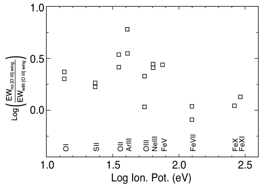
Figure 14: Logarithmic NLR emission line EW ratios vs. ionization potentials. We compare the EWs in the composites with and without a blue wing.

On the other hand, we do see evidence that blue wings are associated with outflows. We might expect that in objects with strong outflows, the gas would be more disturbed, leading to a lower covering factor and thus a lower EW (Baskin & Laor, 2005; Ludwig et al., 2009). We do find that the EW of [O III] in our objects is lower, relative to the AGN power-law continuum, when there is a blue wing in [O III] (Figure 13). The EWs of other low-ionization NLR emission lines are also lower (Figure 14). Furthermore, if we divide the sample into those with and without blue asymmetry in the low-ionization lines (e.g., the $h_{3}$ measurement of [S II]) then we also see low EW narrow-lines in the blue-asymmetric subsample. Thus, we do see indirect evidence that blue wings indicate outflowing material (as we suggested above based on the velocity of the high ionization lines, §6.1). Interestingly enough, all the low-ionization narrow lines, not just [O III], appear to behave similarly, both in terms of EWs and asymmetric lines.

From our sample alone, we see evidence for varying levels of disturbance in the NLR, but we see no direct tie with $L/L_{\mathrm{Edd}}$ or luminosity. Given the limited dynamic range in luminosity, and the large uncertainties on Eddington ratio, it is hard to draw strong conclusions from these data alone. Perhaps the absolute luminosities of the sample are too low (Greene & Ho, 2005b) or the uncertainties on our $L/L_{\mathrm{Edd}}$ estimates are too large.

7 Conclusions

We present observations of a sample of 27 low-mass AGN ($10^{4}~{}M_{\odot}<M_{\mathrm{BH}}<2~{}\times~{}10^{6}~{}M_{\odot}$), observed with the Echellette Spectrograph and Imager on the Keck Telescope. Large samples of low-mass AGN have not existed until recently (Greene & Ho, 2004), and so we compare their emission-line properties to those of well-studied higher-mass AGN.

We investigate the NLR metallicities of these objects using emission line ratios, particularly [N II]$/$H$\alpha$ and [O III]$/$H$\beta$. Our sample includes objects with weaker [N II]$/$H$\alpha$ than higher-mass AGN for a given [O III]$/$H$\beta$, which implies that those objects have lower metallicities. Thus we see some galaxies with similar metallicities to the rare AGN with sub-solar metallicity sought by Groves et al. (2006), yet we cannot determine their metallicities on an absolute scale (e.g. Kewley & Ellison, 2008). Additionally, we do see weak evidence for a correlation between galaxy stellar mass and gas-phase metallicity in these systems. Most likely, the lack of low-metallicity AGN highlighted by Groves et al. (2006) is attributable to the difficulties of finding AGN in low-mass galaxies (e.g. Greene & Ho, 2007a) rather than extra enrichment of the NLR by the AGN itself.

We examine the continuum properties of the accretion disk for our low-mass AGN. By using the emission from the recombination lines [He II] and H$\beta$, we infer the slope of the far-UV continuum from 200–900Å, near the peak of the big blue bump. We find that the far-UV slopes in our low-mass AGN are steeper than those of low-redshift, higher-mass AGN. While we know that our low-mass AGN are very radio-quiet (Greene et al., 2006) and have flat X-ray slopes (Desroches et al., 2009) compared to typical AGN, they have quite similar optical properties and unexpectedly, somewhat steeper UV slopes. These steeper inferred UV continua imply that changing continuum shape could explain the inverse Baldwin effect seen between H$\beta$ FWHM and luminosity (Croom et al., 2002; Greene & Ho, 2005b).

Despite tentative evidence for different SEDs, the NLR structure is also similar between low-mass and typical AGN. Using composite spectra, we are able to measure the widths and velocities of high-ionization Fe lines. As found by Mullaney et al. (2009), the [Fe VII] line exhibits a similar width and blue shift as the blue wing of [O III], pointing to a common physical origin for both transitions in a radially flowing component. As seen in previous work, we find that the width of NLR lines and their blueshift correlates with the ionization potential of the line. We see no evidence for a dramatic change in the NLR structure in this mass and luminosity regime.

Making composite spectra in subsets of luminosity, Eddington ratio, and presence or absence of a blue wing in [O III], we find first that the high-luminosity composite has much broader NLR emission lines than the low-luminosity counterpart within our sample, as has been seen in more-massive AGN. We also find that the subset showing the presence of a blue wing in [O III] exhibits weak NLR emission. We posit that in the objects with a blue wing, the outflow drives gas away from the central region, leading to a lower covering fraction (e.g. Ludwig et al., 2009). However, contrary to our expectations from typical AGN, the presence of a blue wing does not correlate with high Eddington ratio, possibly due to our small dynamic range in this sample. Lastly, we find that the high Eddington ratio composite has excess emission at intermediate velocities in the Balmer lines. This corresponds to the ILR identified by Hu et al. (2008a) and Zhu et al. (2009). This ILR emission could potentially bias $M_{\mathrm{BH}}$ estimates for AGN at high $L/L_{\mathrm{Edd}}$ by decreasing the measured FWHM of the Balmer lines, thus underestimating $M_{\mathrm{BH}}$, as pointed out by Collin et al. (2006) and Zhu et al. (2009).

Overall, the low-mass AGN studied here seem to behave in much the same way as more massive AGN, as traced by optical emission lines. They are likely to have relatively low gas-phase metallicities in the NLR than their larger brethren, and may have steeper far-UV continuum slopes, but the structure and organization of their emission line regions seems to be largely similar.

8 Acknowledgements

We would like to thank Edward L. Robinson and Greg Shields for helpful conversations during the course of this project, and Brent Groves for discussions and help with the MAPPINGS III models. We would also like to thank the referee, for a thorough and insightful report that improved this paper a great deal. Research by A.J.B. is supported by NSF grant AST-1108835. The data presented herein were obtained at the W.M. Keck Observatory, which is operated as a scientific partnership among the California Institute of Technology, the University of California and the National Aeronautics and Space Administration. The Observatory was made possible by the generous financial support of the W.M. Keck Foundation. The authors wish to recognize and acknowledge the very significant cultural role and reverence that the summit of Mauna Kea has always had within the indigenous Hawaiian community. We are most fortunate to have the opportunity to conduct observations from this mountain.

Table 1: Low-Mass AGN Observations

Object	Flag	$z$	S/N	Fit Class
SDSS J010712.03+140844.9	GH01	0.0770	17	AGN
SDSS J024912.86-081525.6	GH02	0.0296	18	AGN
SDSS J032515.59+003408.4	GH03	0.1021	12	AGN
SDSS J080629.80+241955.6		0.0415	31	GAL
SDSS J080907.58+441641.4		0.0540	24	GAL
SDSS J081550.23+250640.9		0.0726	20	GAL
SDSS J082443.28+295923.5		0.0254	54	GAL
SDSS J082912.67+500652.3	GH04	0.0435	37	GAL
SDSS J094310.12+604559.1	GH05	0.0745	25	AGN
SDSS J101108.40+002908.7	GH06	0.1001	12	AGN
SDSS J105755.66+482502.0		0.0732	26	GAL
SDSS J110501.97+594103.6		0.0336	57	GAL
SDSS J114343.76+550019.3		0.0271	26	GAL
SDSS J122342.81+581446.1		0.0146	34	GAL
SDSS J124035.81-002919.4	GH10	0.0810	31	GAL
SDSS J125055.28-015556.6	GH11	0.0815	20	GAL
SDSS J131310.12+051942.1		0.0488	24	GAL
SDSS J141234.67-003500.0	GH13	0.1271	17	AGN
SDSS J143450.62+033842.5	GH14	0.0283	20	GAL
SDSS J153425.59+040806.7		0.0395	9	AGN
SDSS J162636.40+350242.0		0.0341	38	GAL
SDSS J163159.59+243740.2		0.0436	43	GAL
SDSS J170246.09+602818.9	GH16	0.0691	20	GAL
SDSS J172759.15+542147.0	GH17	0.0995	14	AGN
SDSS J215658.30+110343.1		0.1080	39	GAL
SDSS J232159.06+000738.8	GH18	0.1838	12	GAL
SDSS J233837.10-002810.3	GH19	0.0356	29	GAL

Note. —  Low Mass AGN Sample Observations. Col. (1): SDSS Designation. Col (2): Greene & Ho (2004) object designations. Col (3): Redshift. Col. (4): Median S/N per pixel at 5500 Å. Col (5): Fit classification, as described in Section § 3.

Table 2: Fitted Emission Lines

Emission Line	Wavelength (Å)	Possible components
He I, narrow	7065, 6678, 5876	1 G-H Poly each
He I, broad	7065, 6678, 5876	1 Gaussian each
$[$S II]	6730, 6717	1 G-H Poly each
$[$N II]	6584, 6548	1 G-H Poly each
H$\alpha$ – H$\epsilon$, narrow	6563, 4861, 4341, 4102, 3970	1 G-H Poly each
H$\alpha$, broad	6563	$\leq$ 4 Gaussians
$[$O I]	6364, 6300	1 G-H Poly each
$[$O III]	5007, 4959, 4363	$\leq$ 2 G-H Polys each
H$\beta$, broad	4861	$\leq$ 3 Gaussians
He II, narrow	4686	1 G-H Poly
He II, broad	4686	$\leq$ 2 Gaussians
N III	4640	1 Gaussian
H$\gamma$ – H$\epsilon$, broad	4341, 4102, 3970	1 Gaussian each

Note. — Col. (1): Emission Line Species. Col (2): Rest wavelength (Å). Col (3): Possible components in fit, where G-H Poly is a set of Gauss-Hermite functions.

Table 3: Derived Measurements

Object	Log $M_{\mathrm{BH}}/{M}_{\odot}$	Log $L/L_{\mathrm{Edd}}$	Log $M_{\mathrm{gal}}/{M}_{\odot}$	$n_{e}$ (cm-3)	$Z/{Z}_{\odot}$
J0107+1408	$6.03$	$-0.40$	$\cdots$	$360$	$2.0\pm 0.1$
J0249-0815	$5.32$	$-0.66$	$\cdots$	$1010$	$2.0\pm 0.3$
J0325+0034	$5.98$	$-0.57$	$10.05$	$230$	$1.5\pm 0.5$
J0806+2419	$5.95$	$-0.71$	$10.24$	$100$	$1.6\pm 0.2$
J0809+4416	$5.94$	$-0.61$	$10.04$	$140$	$1.8\pm 0.4$
J0815+2506	$5.55$	$-0.50$	$10.24$	$170$	$1.8\pm 0.5$
J0824+2959	$5.33$	$-0.93$	$10.16$	$590$	$1.5\pm 0.2$
J0829+5006	$5.76$	$-0.12$	$\cdots$	$270$	$2.3\pm 0.7$
J0943+6045	$5.76$	$0.02$	$\cdots$	$190$	$1.9\pm 0.2$
J1011+0029	$6.18$	$-0.56$	$\cdots$	$210$	$0.8\pm 0.2$
J1057+4825	$5.68$	$-0.30$	$10.12$	$60$	$0.9\pm 0.1$
J1105+5941	$6.89$	$-1.81$	$10.68$	$440$	$1.5\pm 0.3$
J1143+5500	$5.97$	$-1.25$	$\cdots$	$500$	$0.5\pm 0.1$
J1223+5814	$6.04$	$-0.93$	$9.65$	$850$	$1.6\pm 0.2$
J1240-0029	$5.93$	$-0.09$	$\cdots$	$400$	$1.6\pm 0.4$
J1250-0155	$6.80$	$-1.25$	$\cdots$	$160$	$0.9\pm 0.2$
J1313+0519	$5.32$	$-0.40$	$10.17$	$340$	$2.9\pm 1.0$
J1412-0035	$6.15$	$0.11$	$\cdots$	$1030$	$1.8\pm 0.2$
J1434+0338	$5.65$	$-0.68$	$\cdots$	$240$	$2.5\pm 0.6$
J1534+0408	$4.79$	$-0.21$	$9.36$	$360$	$2.4\pm 0.6$
J1626+3501	$5.54$	$-0.39$	$10.32$	$190$	$2.6\pm 1.4$
J1631+2437	$5.33$	$0.02$	$9.92$	$160$	$2.2\pm 0.8$
J1702+6028	$6.16$	$-0.31$	$\cdots$	$10$	$0.9\pm 0.1$
J1727+5421	$5.68$	$-0.14$	$\cdots$	$290$	$1.6\pm 0.6$
J2156+1103	$6.45$	$-0.65$	$\cdots$	$230$	$0.6\pm 0.1$
J2321+0007	$6.56$	$-0.78$	$\cdots$	$290$	$2.2\pm 0.8$
J2338-0028	$5.92$	$-1.14$	$\cdots$	$540$	$2.0\pm 0.1$

Note. — Col. (1): Object name. Col. (2): Log $M_{\mathrm{BH}}/{M}_{\odot}$, from Xiao et al. (2011). Col. (3): Log $L_{bol}/L_{\mathrm{Edd}}$ calculated from our H$\alpha_{BLR}$ measurements. Col. (4): Log $M_{*}/{M}_{\odot}$ for objects with reported $I$-band luminosities from Greene et al. (2008) (see §4). Col. (5): Density, calculated from the [S II] doublet. Col. (6): $Z/{Z}_{\odot}$, as determined in §4.

Table 4: Emission Line Measurements: H$\alpha$ Region

	[S II] $\lambda 6717$					[S II] $\lambda 6731$		H$\alpha_{NLR}$				[N II] $\lambda 6584$		H$\alpha_{BLR}$
Object	$f/f$(H$\beta$)	FWHM	$h_{3}$	$h_{4}$		$f/f$(H$\beta$)		$f/f$(H$\beta$)	FWHM	$\Delta$v		$f/f$(H$\beta$)		$f/f$(H$\beta$)	FWHM	$\Delta$v
J0107+1408	$0.63\pm 0.04$	$90\pm 20$	$-0.03$	$-0.03$		$0.57\pm 0.04$		$2.6\pm 0.3$	$120\pm 40$	$0$		$0.63\pm 0.04$		$50.6\pm 2.6$	$960\pm 400$	$-10$
J0249-0815	$0.66\pm 0.04$	$110\pm 40$	$0.01$	$0.05$		$0.75\pm 0.05$		$3.8\pm 0.3$	$130\pm 30$	$23$		$0.66\pm 0.04$		$18.3\pm 1.0$	$790\pm 250$	$-68$
J0325+0034	$0.36\pm 0.03$	$120\pm 30$	$-0.08$	$0.01$		$0.30\pm 0.03$		$2.9\pm 0.3$	$150\pm 20$	$0$		$0.36\pm 0.03$		$21.5\pm 0.9$	$1070\pm 190$	$-229$
J0806+2419	$0.36\pm 0.35$	$70\pm 120$	$-0.13$	$0.10$		$0.29\pm 0.28$		$6.0\pm 5.8$	$220\pm 140$	$-2$		$0.68\pm 0.65$		$104.7\pm 100.3$	$1120\pm 210$	$31$
J0809+4416	$0.67\pm 0.02$	$160\pm 10$	$-0.01$	$-0.04$		$0.53\pm 0.02$		$3.4\pm 0.1$	$180\pm 20$	$12$		$0.67\pm 0.02$		$9.7\pm 0.2$	$1020\pm 80$	$81$
J0815+2506	$0.56\pm 0.03$	$130\pm 40$	$-0.10$	$0.04$		$0.45\pm 0.03$		$2.9\pm 0.2$	$150\pm 40$	$0$		$0.56\pm 0.03$		$15.9\pm 0.7$	$840\pm 110$	$-22$
J0824+2959	$0.64\pm 0.02$	$270\pm 10$	$0.05$	$-0.13$		$0.64\pm 0.02$		$6.1\pm 0.2$	$310\pm 10$	$24$		$0.64\pm 0.02$		$3.3\pm 0.1$	$1240\pm 20$	$-236$
J0829+5006	$0.48\pm 0.01$	$150\pm 10$	$0.02$	$-0.05$		$0.41\pm 0.01$		$2.7\pm 0.1$	$160\pm 10$	$0$		$0.48\pm 0.01$		$13.5\pm 0.2$	$690\pm 30$	$-33$
J0943+6045	$>0.29\pm 0.10$	$140\pm 30$	$-0.08$	$-0.02$		$>0.23\pm 0.08$		$>1.4\pm 0.5$	$150\pm 40$	$59$		$>0.45\pm 0.16$		$>48.1\pm 16.1$	$660\pm 420$	$-22$
J1011+0029	$0.20\pm 0.02$	$100\pm 20$	$-0.01$	$0.04$		$0.16\pm 0.02$		$2.7\pm 0.2$	$210\pm 20$	$81$		$0.20\pm 0.02$		$28.8\pm 0.8$	$1220\pm 250$	$46$
J1057+4825	$0.60\pm 0.02$	$80\pm 10$	$-0.04$	$0.06$		$0.44\pm 0.02$		$3.8\pm 0.1$	$70\pm 10$	$23$		$0.60\pm 0.02$		$3.6\pm 0.3$	$640\pm 140$	$-45$
J1105+5941	$0.80\pm 0.02$	$300\pm 20$	$0.07$	$0.06$		$0.74\pm 0.02$		$4.1\pm 0.1$	$350\pm 20$	$0$		$0.80\pm 0.02$		$3.4\pm 0.1$	$4240\pm 780$	$-125$
J1143+5500	$0.61\pm 0.01$	$70\pm 10$	$-0.01$	$0.04$		$0.43\pm 0.01$		$3.3\pm 0.1$	$70\pm 10$	$23$		$0.21\pm 0.01$		$1.1\pm 0.1$	$1290\pm 70$	$-171$
J1223+5814	$0.51\pm 0.01$	$100\pm 10$	$-0.04$	$0.00$		$0.55\pm 0.01$		$4.6\pm 0.1$	$140\pm 20$	$12$		$0.51\pm 0.01$		$12.2\pm 0.2$	$1150\pm 150$	$-22$
J1240-0029	$0.51\pm 0.01$	$140\pm 10$	$-0.01$	$0.03$		$0.47\pm 0.01$		$4.2\pm 0.1$	$160\pm 10$	$0$		$0.51\pm 0.01$		$10.1\pm 0.1$	$840\pm 80$	$-183$
J1250-0155	$0.71\pm 0.01$	$110\pm 10$	$-0.14$	$0.07$		$0.56\pm 0.01$		$3.5\pm 0.1$	$110\pm 10$	$-2$		$0.36\pm 0.01$		$1.9\pm 0.1$	$2260\pm 160$	$11$
J1313+0519	$0.80\pm 0.02$	$150\pm 10$	$-0.01$	$0.03$		$0.71\pm 0.02$		$3.5\pm 0.1$	$180\pm 10$	$0$		$0.80\pm 0.02$		$6.6\pm 0.2$	$720\pm 180$	$-56$
J1412-0035	$>0.30\pm 0.11$	$150\pm 30$	$-0.15$	$0.04$		$>0.35\pm 0.12$		$>2.1\pm 0.8$	$180\pm 40$	$-215$		$>0.53\pm 0.18$		$>57.5\pm 19.2$	$670\pm 370$	$-23$
J1434+0338	$0.64\pm 0.03$	$120\pm 30$	$-0.05$	$0.04$		$0.53\pm 0.03$		$3.4\pm 0.2$	$120\pm 20$	$23$		$0.71\pm 0.02$		$14.4\pm 0.4$	$860\pm 190$	$-68$
J1534+0408	$0.55\pm 0.07$	$70\pm 20$	$0.01$	$0.00$		$0.49\pm 0.07$		$3.0\pm 0.4$	$100\pm 10$	$10$		$0.55\pm 0.07$		$34.4\pm 3.5$	$480\pm 130$	$24$
J1626+3501	$0.40\pm 0.02$	$70\pm 20$	$-0.02$	$-0.03$		$0.32\pm 0.01$		$3.6\pm 0.1$	$90\pm 10$	$23$		$0.68\pm 0.02$		$24.2\pm 0.5$	$750\pm 40$	$-45$
J1631+2437	$0.56\pm 0.02$	$180\pm 20$	$0.02$	$0.07$		$0.45\pm 0.02$		$3.4\pm 0.1$	$210\pm 20$	$0$		$0.56\pm 0.02$		$10.5\pm 0.2$	$600\pm 140$	$-332$
J1702+6028	$0.47\pm 0.02$	$180\pm 30$	$-0.06$	$-0.15$		$0.33\pm 0.02$		$4.5\pm 0.2$	$260\pm 20$	$-22$		$0.48\pm 0.02$		$31.5\pm 0.9$	$1040\pm 160$	$-321$
J1727+5421	$0.41\pm 0.02$	$150\pm 60$	$-0.08$	$-0.01$		$0.35\pm 0.01$		$3.1\pm 0.2$	$200\pm 70$	$0$		$0.41\pm 0.02$		$12.3\pm 0.3$	$810\pm 690$	$12$
J2156+1103	$0.18\pm 0.01$	$160\pm 30$	$-0.08$	$-0.01$		$0.15\pm 0.01$		$2.8\pm 0.1$	$190\pm 20$	$11$		$0.24\pm 0.01$		$6.7\pm 0.1$	$1540\pm 230$	$120$
J2321+0007	$0.65\pm 0.06$	$180\pm 110$	$-0.05$	$-0.01$		$0.56\pm 0.07$		$3.6\pm 0.3$	$200\pm 80$	$12$		$0.65\pm 0.05$		$27.5\pm 1.4$	$1670\pm 1020$	$-114$
J2338-0028	$1.22\pm 0.01$	$120\pm 10$	$0.01$	$0.07$		$1.19\pm 0.01$		$3.8\pm 0.1$	$130\pm 10$	$12$		$1.22\pm 0.01$		$2.6\pm 0.1$	$1490\pm 80$	$-33$

Note. — Col. (1): Object name. Cols. (2-6): Fitting parameters for [S II] $\lambda 6717$. Col. (7): Flux of [S II] $\lambda 6731$, where all other parameters are fixed to [S II] $\lambda 6717$. Cols. (8-10): Fitting parameters for H$\alpha_{NLR}$, where $h_{\mathrm{3}}$ and $h_{\mathrm{4}}$ are fixed to [S II] $\lambda 6717$, and $\Delta$v is the centroid shift compared to [S II]. Col. (11): Flux of [N II], where all other parameters are fixed. Cols. (12-14): Parametric measurements for total H$\alpha_{\mathrm{BLR}}$ fit. FWHMs and $\Delta$v are in km s^-1, and fluxes are relative to H$\beta_{NLR}$, which can be found in Table 5. Fluxes have been corrected for Galactic extinction using values from Schlegel et al. (1998) and the reddening law of O’Donnell (1994). Upper and lower limits are three sigma estimates.

Table 5: Emission Line Measurements: H$\beta$ Region

	[0 III] $\lambda 5007$				H$\beta_{NLR}$				He II $\lambda 4686_{NLR}$				H$\beta_{BLR}$
Object	$f/f$(H$\beta$)	FWHM	$\Delta$v		$F$(H$\beta$)	FWHM	$\Delta$v		$f/f$(H$\beta$)	FWHM	$\Delta$v		$f/f$(H$\beta$)	FWHM	$\Delta$v
J0107+1408	$12.9\pm 0.7$	$150\pm 10$	$7$		$0.14\pm 0.01$	$160\pm 30$	$30$		$0.29\pm 0.05$	$150\pm 30$	$1.2$		$14.3\pm 0.8$	$1380\pm 330$	$18$
J0249-0815	$11.1\pm 0.6$	$110\pm 10$	$30$		$0.15\pm 0.01$	$160\pm 30$	$41$		$0.33\pm 0.05$	$150\pm 30$	$1.3$		$4.7\pm 0.3$	$1190\pm 380$	$-15$
J0325+0034	$6.3\pm 0.3$	$100\pm 10$	$7$		$0.13\pm 0.01$	$400\pm 20$	$-4$		$0.16\pm 0.04$	$380\pm 20$	$12.7$		$3.8\pm 0.2$	$3120\pm 260$	$375$
J0806+2419	$12.0\pm 11.5$	$180\pm 20$	$-24$		$0.08\pm 0.06$	$230\pm 1250$	$24$		$0.13\pm 0.29$	$220\pm 1250$	$11.5$		$38.4\pm 36.9$	$1530\pm 670$	$14$
J0809+4416	$3.2\pm 0.1$	$160\pm 10$	$-4$		$0.56\pm 0.01$	$190\pm 20$	$41$		$0.10\pm 0.02$	$180\pm 20$	$1.2$		$2.8\pm 0.1$	$1550\pm 280$	$179$
J0815+2506	$3.6\pm 0.2$	$130\pm 20$	$18$		$0.11\pm 0.01$	$180\pm 40$	$30$		$0.14\pm 0.03$	$170\pm 40$	$1.3$		$4.4\pm 0.2$	$1410\pm 440$	$30$
J0824+2959	$16.8\pm 0.3$	$360\pm 10$	$38$		$2.83\pm 0.03$	$340\pm 10$	$32$		$0.15\pm 0.01$	$320\pm 10$	$-0.2$		$0.8\pm 0.1$	$730\pm 90$	$-32$
J0829+5006	$6.3\pm 0.1$	$180\pm 10$	$18$		$1.56\pm 0.01$	$200\pm 10$	$18$		$0.17\pm 0.01$	$190\pm 10$	$1.3$		$3.0\pm 0.1$	$1040\pm 40$	$18$
J0943+6045	$>4.4\pm 1.5$	$190\pm 20$	$-19$		$<0.27\pm 0.08$	$160\pm 40$	$47$		$>0.53\pm 0.18$	$600\pm 40$	$26.9$		$>14.6\pm 4.9$	$760\pm 240$	$47$
J1011+0029	$4.4\pm 0.2$	$160\pm 10$	$30$		$0.19\pm 0.01$	$360\pm 30$	$110$		$0.43\pm 0.03$	$340\pm 30$	$1.3$		$7.3\pm 0.3$	$1690\pm 290$	$87$
J1057+4825	$1.7\pm 0.1$	$300\pm 50$	$-96$		$0.34\pm 0.01$	$80\pm 20$	$41$		$0.01\pm 0.01$	$80\pm 20$	$12.9$		$0.6\pm 1.5$	$720\pm 1090$	$-4$
J1105+5941	$2.5\pm 0.1$	$400\pm 30$	$-4$		$6.10\pm 0.03$	$370\pm 20$	$30$		$0.03\pm 0.01$	$350\pm 20$	$1.2$		$0.8\pm 0.1$	$6740\pm 1980$	$594$
J1143+5500	$1.5\pm 0.1$	$70\pm 10$	$30$		$1.07\pm 0.01$	$80\pm 10$	$53$		$0.01\pm 0.01$	$70\pm 10$	$1.4$		$0.1\pm 0.1$	$460\pm 10$	$317$
J1223+5814	$12.3\pm 0.2$	$100\pm 10$	$18$		$1.40\pm 0.01$	$160\pm 10$	$30$		$0.31\pm 0.01$	$150\pm 10$	$1.3$		$1.9\pm 0.1$	$1730\pm 400$	$41$
J1240-0029	$7.4\pm 0.1$	$150\pm 10$	$18$		$1.99\pm 0.01$	$170\pm 10$	$30$		$0.14\pm 0.01$	$160\pm 10$	$1.2$		$2.4\pm 0.1$	$1130\pm 100$	$-130$
J1250-0155	$4.0\pm 0.1$	$150\pm 10$	$5$		$1.79\pm 0.01$	$120\pm 10$	$26$		$0.07\pm 0.01$	$110\pm 10$	$4.8$		$0.6\pm 0.1$	$10170\pm 6670$	$563$
J1313+0519	$5.0\pm 0.1$	$160\pm 10$	$-4$		$0.48\pm 0.01$	$200\pm 10$	$30$		$0.14\pm 0.01$	$190\pm 10$	$1.3$		$1.3\pm 0.1$	$1110\pm 260$	$-4$
J1412-0035	$>5.4\pm 1.9$	$190\pm 10$	$-21$		$<0.16\pm 0.04$	$120\pm 30$	$-288$		$>0.07\pm 0.05$	$110\pm 30$	$4.8$		$>19.4\pm 6.5$	$950\pm 400$	$8$
J1434+0338	$6.1\pm 0.2$	$140\pm 10$	$-4$		$0.31\pm 0.01$	$150\pm 20$	$41$		$0.16\pm 0.03$	$140\pm 20$	$1.2$		$2.8\pm 0.1$	$1220\pm 270$	$64$
J1534+0408	$6.7\pm 0.7$	$80\pm 10$	$18$		$0.05\pm 0.01$	$200\pm 20$	$40$		$0.13\pm 0.08$	$190\pm 10$	$8.6$		$9.5\pm 1.0$	$500\pm 210$	$49$
J1626+3501	$3.7\pm 0.1$	$90\pm 130$	$18$		$0.36\pm 0.01$	$100\pm 10$	$53$		$0.12\pm 0.02$	$100\pm 10$	$1.3$		$3.9\pm 0.2$	$910\pm 150$	$7$
J1631+2437	$6.2\pm 0.1$	$210\pm 10$	$18$		$2.13\pm 0.03$	$220\pm 20$	$30$		$0.13\pm 0.02$	$210\pm 20$	$1.2$		$3.2\pm 0.1$	$400\pm 50$	$-326$
J1702+6028	$4.4\pm 0.2$	$200\pm 10$	$-27$		$0.76\pm 0.02$	$420\pm 30$	$-39$		$0.13\pm 0.03$	$400\pm 30$	$24.2$		$5.6\pm 0.2$	$3890\pm 940$	$-15$
J1727+5421	$5.3\pm 0.2$	$170\pm 20$	$18$		$0.64\pm 0.01$	$250\pm 40$	$30$		$0.24\pm 0.02$	$240\pm 40$	$1.4$		$2.8\pm 0.1$	$1300\pm 690$	$53$
J2156+1103	$0.5\pm 0.1$	$440\pm 170$	$-201$		$1.82\pm 0.01$	$220\pm 20$	$45$		$<0.31\pm 0.11$	$50\pm 20$	$\cdots$		$1.0\pm 0.2$	$4260\pm 470$	$-408$
J2321+0007	$4.5\pm 0.3$	$210\pm 40$	$-15$		$0.08\pm 0.01$	$250\pm 70$	$30$		$0.21\pm 0.04$	$230\pm 70$	$1.2$		$8.3\pm 0.5$	$3930\pm 1200$	$76$
J2338-0028	$13.6\pm 0.1$	$120\pm 10$	$30$		$1.29\pm 0.01$	$140\pm 10$	$41$		$0.37\pm 0.01$	$130\pm 10$	$1.2$		$0.5\pm 0.1$	$1200\pm 470$	$7$

Note. — Col. (1): Object name. Cols. (2-4): Parametric measurements for total [O III] $\lambda{5007}$ fit. Cols. (5-7): Fitting parameters for H$\beta_{NLR}$. Note that $F$(H$\beta$) is in units of $10^{-15}~{}$ergs s^-1 cm^-2 Å^-1, and $h_{\mathrm{3}}$ and $h_{\mathrm{4}}$ are fixed to [S II] $\lambda 6717$. Cols. (8-10): Fitting parameters for [He II]_NLR, $h_{\mathrm{3}}$ and $h_{\mathrm{4}}$ are fixed to [S II] $\lambda 6717$. Cols. (11-13): Parametric measurements for total H$\beta_{BLR}$ fit. FWHMs and $\Delta$v are in km s^-1, and fluxes are relative to H$\beta_{NLR}$. Fluxes have been corrected for Galactic extinction using values from Schlegel et al. (1998) and the reddening law of O’Donnell (1994). Upper and lower limits are three sigma estimates.

Figure 4: Left column. H$\beta$ fits, where dotted purple lines show narrow components of H$\beta$, He II and [O III]. Blue, cyan, and green lines are broad components of H$\beta$, He II, and N III. Right column. H$\alpha$ fits, where dotted purple lines are [N II] and H$\alpha_{\mathrm{NLR}}$ fits, and blue, cyan, and green show components of H$\alpha_{\mathrm{BLR}}$. In the insets we zoom in on the [S II] fit. For both columns, the panels show (from top to bottom) J0824+2959, J0806+2419, J1105+5941, and J0829+5006.

Figure 8: Distribution of derived UV slope, from He II to H$\beta$ ratio, for the GH objects (solid) and the Ho & Kim sample (dotted).

Figure 9: Continuum-subtracted composite spectrum of low-mass AGN showing weak emission line features listed in Table 6.

Table 6: Composite NLR Emission Lines

Line	$\lambda$	FWHM	$f/f_{\mathrm{H}\beta}$	Ion. Pot.
$[$Ne III]	3868.7	165	0.42	63.5
$[$Fe V]	3889.0	100	0.07	75.0
$[$Ne III]	3967.2	153	0.03	63.5
H$\epsilon$	3970.2	112	0.06	13.6
$[$S II]	4068.9	150	0.04	23.3
H$\delta$	4101.9	112	0.16	13.6
H$\gamma$	4340.6	112	0.26	13.6
$[$O III]	4362.9	158	0.13	54.9
He II	4685.9	199	0.19	54.4
H$\beta$	4861.1	208	1.00	13.6
$[$O III]	5006.7	157	4.35	54.9
$[$Fe VII]	5720.3	272	0.03	125.0
He I	5875.8	115	0.09	24.5
$[$Fe VII]	6085.6	223	0.05	125.0
$[$O I]	6300.3	112	0.19	13.6
$[$O I]	6364.1	112	0.07	13.6
$[$Fe X]	6371.4	459	0.05	262.1
$[$N II]	6548.1	162	0.38	29.6
H$\alpha$	6563.0	111	2.02	13.6
He I	6678.2	115	0.02	24.5
$[$S II]	6716.7	112	0.48	23.3
$[$S II]	6731.1	112	0.44	23.3
He I	7065.3	115	0.03	24.5
$[$Ar III]	7135.8	105	0.09	40.7
$[$Ar III]	7751.6	106	0.01	40.7
$[$O II]	7320.1	160	0.04	35.1
$[$O II]	7330.1	126	0.02	35.1
$[$Fe XI]	7890.5	332	0.05	290.2
$[$O I]	8445.5	255	0.06	13.6
$[$S III]	9069.1	104	0.32	34.8
$[$S III]	9531.0	125	0.63	34.8

Note. — Narrow emission-line measurements of continuum-subtracted composite spectrum of low-mass AGN. Col. (1): Line ID. Col. (2): Measured centroid in Å. Col. (3): FWHM in km s^-1. Col. (4): Flux relative to narrow H$\beta$. Col. (5): Ionization potential in eV.

Table 7: Subset Properties

		Ave. $\sigma$ (km s-1)
Composite	No. of objects	All NLR	High-ion Fe
Whole sample	27	70	135
High $L_{bol}$	14	98	188
Low $L_{bol}$	13	53	98
High $L_{bol}/L_{Edd}$	14	90	175
Low $L_{bol}/L_{Edd}$	13	55	102
Includes [O III] Wing	17	85	136
No [O III] Wing	10	66	131

Note. — NLR emission-line properties for subset composites. Averages are taken over all measured NLR emission lines, or over high-ionization Fe lines (ionization potential $>100$ eV) as noted.

Figure 12: Composites of the H$\alpha$ (left panel) and H$\beta$ regions (right panel) for high $L/L_{\mathrm{Edd}}$ (solid) and low $L/L_{\mathrm{Edd}}$ (dotted) objects. Notice the excess ILR in the high $L/L_{\mathrm{Edd}}$ composite for both lines.

Figure 13: Composite spectra with a blue wing in [O III] (solid) and without (dotted). In order to compare EWs, we plot each continuum-subtracted composite plus the average power-law AGN continuum of objects in that composite, where the power law is normalized to 5600 Å. Note that symmetric [O III] lines have much higher EW.

References

- Adelman-McCarthy et al. (2006) Adelman-McCarthy, J. K., Agüeros, M. A., Allam, S. S., et al. 2006, ApJS, 162, 38
- Asplund et al. (2004) Asplund, M., Grevesse, N., Sauval, A. J., Allende Prieto, C., & Kiselman, D. 2004, A&A, 417, 751
- Baldwin et al. (1981) Baldwin, J. A., Phillips, M. M., & Terlevich, R. 1981, PASP, 93, 5
- Barth et al. (2005) Barth, A. J., Greene, J. E., & Ho, L. C. 2005, ApJ, 619, L151
- Barth et al. (2008) —. 2008, AJ, 136, 1179
- Barth et al. (2004) Barth, A. J., Ho, L. C., Rutledge, R. E., & Sargent, W. L. W. 2004, ApJ, 607, 90
- Baskin & Laor (2005) Baskin, A. & Laor, A. 2005, MNRAS, 358, 1043
- Bell et al. (2003) Bell, E. F., McIntosh, D. H., Katz, N., & Weinberg, M. D. 2003, ApJS, 149, 289
- Bentz et al. (2006) Bentz, M. C., Peterson, B. M., Pogge, R. W., Vestergaard, M., & Onken, C. A. 2006, ApJ, 644, 133
- Bonning et al. (2007) Bonning, E. W., Cheng, L., Shields, G. A., Salviander, S., & Gebhardt, K. 2007, ApJ, 659, 211
- Boroson (2005) Boroson, T. 2005, AJ, 130, 381
- Boroson (2002) Boroson, T. A. 2002, ApJ, 565, 78
- Boroson & Green (1992) Boroson, T. A. & Green, R. F. 1992, ApJS, 80, 109
- Brinchmann et al. (2004) Brinchmann, J., Charlot, S., White, S. D. M., et al. 2004, MNRAS, 351, 1151
- Bromm & Yoshida (2011) Bromm, V. & Yoshida, N. 2011, ARA&A, 49, 373
- Bruzual & Charlot (2003) Bruzual, G. & Charlot, S. 2003, MNRAS, 344, 1000
- Calzetti et al. (2000) Calzetti, D., Armus, L., Bohlin, R. C., et al. 2000, ApJ, 533, 682
- Cecil et al. (2002) Cecil, G., Dopita, M. A., Groves, B., et al. 2002, ApJ, 568, 627
- Chabrier (2003) Chabrier, G. 2003, PASP, 115, 763
- Collin et al. (2006) Collin, S., Kawaguchi, T., Peterson, B. M., & Vestergaard, M. 2006, A&A, 456, 75
- Cooke et al. (1976) Cooke, B. A., Elvis, M., Ward, M. J., et al. 1976, MNRAS, 177, 121P
- Croom et al. (2002) Croom, S. M., Rhook, K., Corbett, E. A., et al. 2002, MNRAS, 337, 275
- Davis et al. (2007) Davis, S. W., Woo, J.-H., & Blaes, O. M. 2007, ApJ, 668, 682
- De Robertis & Osterbrock (1984) De Robertis, M. M. & Osterbrock, D. E. 1984, ApJ, 286, 171
- Desroches et al. (2009) Desroches, L., Greene, J. E., & Ho, L. C. 2009, ApJ, 698, 1515
- Done et al. (2012) Done, C., Davis, S. W., Jin, C., Blaes, O., & Ward, M. 2012, MNRAS, 420, 1848
- Dong et al. (2012) Dong, X.-B., Ho, L. C., Yuan, W., et al. 2012, ApJ, in press (arXiv:1206.3843)
- Dopita et al. (1982) Dopita, M. A., Binette, L., & Schwartz, R. D. 1982, ApJ, 261, 183
- Dopita et al. (2002) Dopita, M. A., Groves, B. A., Sutherland, R. S., Binette, L., & Cecil, G. 2002, ApJ, 572, 753
- Evans (1986) Evans, I. N. 1986, ApJ, 309, 544
- Filippenko & Halpern (1984) Filippenko, A. V. & Halpern, J. P. 1984, ApJ, 285, 458
- Filippenko & Ho (2003) Filippenko, A. V. & Ho, L. C. 2003, ApJ, 588, L13
- Francis et al. (1991) Francis, P. J., Hewett, P. C., Foltz, C. B., et al. 1991, ApJ, 373, 465
- Frank et al. (2002) Frank, J., King, A., & Raine, D. J. 2002, Accretion Power in Astrophysics: Third Edition, ed. Frank, J., King, A., & Raine, D. J.
- Gelbord et al. (2009) Gelbord, J. M., Mullaney, J. R., & Ward, M. J. 2009, MNRAS, 397, 172
- Grandi (1978) Grandi, S. A. 1978, ApJ, 221, 501
- Greene & Ho (2004) Greene, J. E. & Ho, L. C. 2004, ApJ, 610, 722
- Greene & Ho (2005a) —. 2005a, ApJ, 627, 721
- Greene & Ho (2005b) —. 2005b, ApJ, 630, 122
- Greene & Ho (2007a) —. 2007a, ApJ, 670, 92
- Greene & Ho (2007b) —. 2007b, ApJ, 656, 84
- Greene et al. (2008) Greene, J. E., Ho, L. C., & Barth, A. J. 2008, ApJ, 688, 159
- Greene et al. (2006) Greene, J. E., Ho, L. C., & Ulvestad, J. S. 2006, ApJ, 636, 56
- Greene et al. (2009) Greene, J. E., Zakamska, N. L., Liu, X., Barth, A. J., & Ho, L. C. 2009, ApJ, 702, 441
- Greene et al. (2012) Greene, J. E., Zakamska, N. L., & Smith, P. S. 2012, ApJ, 746, 86
- Groves (2007) Groves, B. 2007, in Astronomical Society of the Pacific Conference Series, Vol. 373, The Central Engine of Active Galactic Nuclei, ed. L. C. Ho & J.-W. Wang, 511–+
- Groves & Allen (2010) Groves, B. A. & Allen, M. G. 2010, New A, 15, 614
- Groves et al. (2004a) Groves, B. A., Dopita, M. A., & Sutherland, R. S. 2004a, ApJS, 153, 9
- Groves et al. (2004b) —. 2004b, ApJS, 153, 75
- Groves et al. (2006) Groves, B. A., Heckman, T. M., & Kauffmann, G. 2006, MNRAS, 371, 1559
- Gültekin et al. (2009) Gültekin, K., Richstone, D. O., Gebhardt, K., et al. 2009, ApJ, 698, 198
- Hainline et al. (2011) Hainline, K. N., Shapley, A. E., Greene, J. E., & Steidel, C. C. 2011, ApJ, 733, 31
- Hamann & Ferland (1999) Hamann, F. & Ferland, G. 1999, ARA&A, 37, 487
- Hao et al. (2005) Hao, L., Strauss, M. A., Tremonti, C. A., et al. 2005, AJ, 129, 1783
- Heckman et al. (1981) Heckman, T. M., Miley, G. K., van Breugel, W. J. M., & Butcher, H. R. 1981, ApJ, 247, 403
- Henry & Worthey (1999) Henry, R. B. C. & Worthey, G. 1999, PASP, 111, 919
- Ho (2009) Ho, L. C. 2009, ApJ, 699, 638
- Ho et al. (1997a) Ho, L. C., Filippenko, A. V., & Sargent, W. L. W. 1997a, ApJS, 112, 315
- Ho et al. (2003) —. 2003, ApJ, 583, 159
- Ho et al. (1997b) Ho, L. C., Filippenko, A. V., Sargent, W. L. W., & Peng, C. Y. 1997b, ApJS, 112, 391
- Ho & Kim (2009) Ho, L. C. & Kim, M. 2009, ApJS, 184, 398
- Hu et al. (2008a) Hu, C., Wang, J., Ho, L. C., et al. 2008a, ApJ, 683, L115
- Hu et al. (2008b) Hu, C., Wang, J.-M., Ho, L. C., et al. 2008b, ApJ, 687, 78
- Husemann et al. (2011) Husemann, B., Wisotzki, L., Jahnke, K., & Sánchez, S. F. 2011, A&A, 535, A72
- Izotov & Thuan (2008) Izotov, Y. I., & Thuan, T. X. 2008, ApJ, 687, 133
- Jiang et al. (2011) Jiang, Y.-F., Greene, J. E., Ho, L. C., Xiao, T., & Barth, A. J. 2011, ApJ, 742, 68
- Kauffmann et al. (2003) Kauffmann, G., Heckman, T. M., Tremonti, C., et al. 2003, MNRAS, 346, 1055
- Kewley & Ellison (2008) Kewley, L. J. & Ellison, S. L. 2008, ApJ, 681, 1183
- Kinney et al. (2000) Kinney, A. L., Schmitt, H. R., Clarke, C. J., et al. 2000, ApJ, 537, 152
- Komossa et al. (2008) Komossa, S., Xu, D., Zhou, H., Storchi-Bergmann, T., & Binette, L. 2008, ApJ, 680, 926
- Kovačević et al. (2010) Kovačević, J., Popović, L. Č., & Dimitrijević, M. S. 2010, ApJS, 189, 15
- Kraemer et al. (1999) Kraemer, S. B., Ho, L. C., Crenshaw, D. M., Shields, J. C., & Filippenko, A. V. 1999, ApJ, 520, 564
- Leighly & Moore (2006) Leighly, K. M. & Moore, J. R. 2006, ApJ, 644, 748
- Ludwig et al. (2009) Ludwig, R. R., Wills, B., Greene, J. E., & Robinson, E. L. 2009, ApJ, 706, 995
- Milosavljević et al. (2009) Milosavljević, M., Couch, S. M., & Bromm, V. 2009, ApJ, 696, L146
- Miniutti et al. (2009) Miniutti, G., Ponti, G., Greene, J. E., et al. 2009, MNRAS, 394, 443
- Mullaney et al. (2009) Mullaney, J. R., Ward, M. J., Done, C., Ferland, G. J., & Schurch, N. 2009, MNRAS, 394, L16
- Müller-Sánchez et al. (2011) Müller-Sánchez, F., Prieto, M. A., Hicks, E. K. S., et al. 2011, ApJ, 739, 69
- Netzer (1990) Netzer, H. 1990, in Active Galactic Nuclei, ed. R. D. Blandford, H. Netzer, L. Woltjer, T. J.-L. Courvoisier, & M. Mayor, 57–160
- Netzer & Trakhtenbrot (2007) Netzer, H. & Trakhtenbrot, B. 2007, ApJ, 654, 754
- O’Donnell (1994) O’Donnell, J. E. 1994, ApJ, 422, 158
- Osterbrock & Ferland (2006) Osterbrock, D. E. & Ferland, G. J. 2006, Astrophysics of gaseous nebulae and active galactic nuclei, ed. Osterbrock, D. E. & Ferland, G. J.
- Osterbrock & Mathews (1986) Osterbrock, D. E. & Mathews, W. G. 1986, ARA&A, 24, 171
- Osterbrock & Pogge (1985) Osterbrock, D. E. & Pogge, R. W. 1985, ApJ, 297, 166
- Pagel & Edmunds (1981) Pagel, B. E. J. & Edmunds, M. G. 1981, ARA&A, 19, 77
- Penston & Fosbury (1978) Penston, M. V. & Fosbury, R. A. E. 1978, MNRAS, 183, 479
- Penston et al. (1984) Penston, M. V., Fosbury, R. A. E., Boksenberg, A., Ward, M. J., & Wilson, A. S. 1984, MNRAS, 208, 347
- Pettini & Pagel (2004) Pettini, M. & Pagel, B. E. J. 2004, MNRAS, 348, L59
- Phillips et al. (1983) Phillips, M. M., Charles, P. A., & Baldwin, J. A. 1983, ApJ, 266, 485
- Proga et al. (2000) Proga, D., Stone, J. M., & Kallman, T. R. 2000, ApJ, 543, 686
- Richards et al. (2003) Richards, G. T., Hall, P. B., Vanden Berk, D. E., et al. 2003, AJ, 126, 1131
- Rodríguez-Ardila et al. (2011) Rodríguez-Ardila, A., Prieto, M. A., Portilla, J. G., & Tejeiro, J. M. 2011, ApJ, 743, 100
- Salviander et al. (2007) Salviander, S., Shields, G. A., Gebhardt, K., & Bonning, E. W. 2007, ApJ, 662, 131
- Schlegel et al. (1998) Schlegel, D. J., Finkbeiner, D. P., & Davis, M. 1998, ApJ, 500, 525
- Schmitt et al. (2003) Schmitt, H. R., Donley, J. L., Antonucci, R. R. J., et al. 2003, ApJ, 597, 768
- Shang et al. (2005) Shang, Z., Brotherton, M. S., Green, R. F., et al. 2005, ApJ, 619, 41
- Sheinis et al. (2002) Sheinis, A. I., Bolte, M., Epps, H. W., et al. 2002, PASP, 114, 851
- Shields (1978) Shields, G. A. 1978, Nature, 272, 706
- Sutherland & Dopita (1993) Sutherland, R. S. & Dopita, M. A. 1993, ApJS, 88, 253
- Tremaine et al. (2002) Tremaine, S., Gebhardt, K., Bender, R., et al. 2002, ApJ, 574, 740
- Tremonti et al. (2004) Tremonti, C. A., Heckman, T. M., Kauffmann, G., et al. 2004, ApJ, 613, 898
- Vanden Berk et al. (2001) Vanden Berk, D. E., Richards, G. T., Bauer, A., et al. 2001, AJ, 122, 549
- Verner (2000) Verner, E. 2000, PhD thesis, UNIVERSITY OF TORONTO (CANADA)
- Vestergaard & Wilkes (2001) Vestergaard, M. & Wilkes, B. J. 2001, ApJS, 134, 1
- Volonteri & Natarajan (2009) Volonteri, M. & Natarajan, P. 2009, MNRAS, 400, 1911
- Wang & Wei (2009) Wang, J. & Wei, J. Y. 2009, ApJ, 696, 741
- Ward & Morris (1984) Ward, M. & Morris, S. 1984, MNRAS, 207, 867
- Whittle (1985) Whittle, M. 1985, MNRAS, 213, 33
- Whittle (1992) —. 1992, ApJS, 79, 49
- Xiao et al. (2011) Xiao, T., Barth, A. J., Greene, J. E., et al. 2011, ApJ, 739, 28
- York et al. (2000) York, D. G., Adelman, J., Anderson, Jr., J. E., et al. 2000, AJ, 120, 1579
- Zhu et al. (2009) Zhu, L., Zhang, S. N., & Tang, S. 2009, ApJ, 700, 1173