Measuring capital market efficiency: Global and local correlations structure

Abstract

We introduce a new measure for the capital market efficiency. The measure takes into consideration the correlation structure of the returns (long-term and short-term memory) and local herding behavior (fractal dimension). The efficiency measure is taken as a distance from an ideal efficient market situation. Methodology is applied to a portfolio of 41 stock indices. We find that the Japanese NIKKEI is the most efficient market. From geographical point of view, the more efficient markets are dominated by the European stock indices and the less efficient markets cover mainly Latin America, Asia and Oceania. The inefficiency is mainly driven by a local herding, i.e. a low fractal dimension.

PACS codes: 05.45.Tp, 89.65.Gh

1 Introduction

A concept of the capital market efficiency is a central notion in the financial markets theory [21, 22]. This notion is generally used for an ideal image of the capital market enabling to process relevant information to the fundamental price generation. If the relevant information to the fundamental price generation is completely processed by the capital market price mechanism, then such capital market is called to be efficient. Thus the capital market efficiency accentuates the informational efficiency of capital markets. A notion of the efficient capital market represents such capital market where prices on traded securities, e.g. stocks, bonds, or property, already reflect all available information and that investors are completely rational. Consequently, the notion of the efficient capital market represents fair game pattern. No investor can have an advantage in predicting a return on an asset price, since no one has access to information not already available to everyone. It means that investors in the efficient capital market cannot expect to achieve abnormal returns systematically. In other words, the capital market is efficient if the fluctuations of returns are unpredictable [21, 22, 35].

Paradoxically, an achievement of the ideal efficient capital market, enabling efficient allocation of investments, brings about no activity of investors and no activity of speculators. Because real life experiences with capital markets have shown that there are investors who indeed have been beating the capital markets in long-term, discrepancies from the above mentioned ideal state are existent and thus worth analyzing.

Testing the efficiency of various capital markets in different regions is a popular topic in financial journals (e.g. [33, 34, 2, 16, 15]). However, the hypothesis of market efficiency is standardly either rejected or not and markets are ranked quite infrequently. Moreover, the researchers majorly focus on a single method and comment on the results. And even further, the whole idea of testing or measuring capital market efficiency has been dealing with the joint-hypothesis problem (i.e. when we reject the efficiency of a specific market, it might be caused by a wrong assumption of the market’s behavior) since its beginnings. This issue was also touched by Fama himself [22]. In this paper, we try to bypass the problem by defining the efficient market as a martingale. We then analyze fractal dimension, and long-range and short-range dependence to describe and measure the efficiency of specific markets.

Hurst exponent and a presence of long-term memory has been widely analyzed in recent years – in stock indices [17, 29], interest rates [12], bonds [13], exchange rates [45] and others. The results vary depending on asset type and on geographical situation as well. Statistically significant long-range dependence was detected in some individual NYSE-listed stocks [5]. Even though the series of developed markets usually posses only short or no memory, emerging markets exhibit a different behavior [47, 44]. Looking at a different frequency, a significantly long memory was found for weekly returns of a large number of Greek stocks [40]. Cajueiro & Tabak [8] rank the markets according to their efficiency and suggest that Hong Kong stock exchange is the most efficient one followed by Chinese A type shares and Singapore and finally by Chinese B type shares, which indicates that liquidity and capital restrictions should be taken into consideration in efficiency testing and mainly interpretation.

We use the Hurst exponent $H$ and the fractal dimension $D$ to construct a new measure of market efficiency based on a deviation from the ideal state (the efficient market) from both local and global perspective. If the results based on different measures vary, we can further distinguish between local (herding) and global (correlations structure) effects. We use the fact that the measures are bounded and thus can be used to construct an informative norm representing the said deviation from the ideal state. The measure is estimated for 41 stock indices at different stages of development from the beginning of 2000 till the end of August 2011, i.e. the data set includes the DotCom bubble and its bursting as well as the current Global Financial Crisis.

The paper is structured as follows. In Section 2, we define the efficient capital market. Section 3 describes relationships between efficiency and the measures we use. In Section 4, we describe the methods used for the fractal dimension and Hurst exponent estimation. Section 5 covers the results and discusses the implications. Section 6 concludes. The main value of this paper lies in the fact that the proposed methodology bypasses the standard caveats of efficiency testing by building on the martingale definition of efficiency, using different methods and merging them into the efficiency measure. Such rather bold path leads to very interesting and also meaningful results.

2 Capital market efficiency

We use a triple $(\Omega,\mathscr{T},P)$ for expressing a probability space and the expression $\mathbb{E}[X|\mathscr{T}]$ for the conditional expectations. Let $\{\omega\in\Omega\}$ be a set of elementary market situations. Let $\mathscr{T}$ be some $\sigma$-algebra of the subsets of $\Omega$, $P$ is a probability measure on $\mathscr{T}$ and $\Omega$ is an information set. This structure gives us all the machinery for static situations involving randomness. For dynamic situations, involving randomness over time, a sequence of $\sigma$-algebras $\{\mathscr{T}_{t},t\geq 0\}$ needs to be taken into consideration. Inclusion $\mathscr{T}_{t}\subset\mathscr{T}_{t+1}$ for all $t$ represents the information arriving in time $t$. Suppose all $\sigma$-algebras to be complete. Thus $\mathscr{T}_{0}$ represents initial information. On the other hand, a situation that all is known is represented by the expression $\mathscr{T}_{\infty}=\lim_{t\rightarrow\infty}\mathscr{T}_{t}$. Such a family $\{\mathscr{T}_{t\geq 0}\}$ is called a filtration; a probability space endowed with such a filtration, $(\Omega,\mathscr{T},\{\mathscr{T}_{t}\},P)$, is also called a stochastic basis.

Let $C=(\Omega,\mathscr{T},\{\mathscr{T}_{t}\},P)$ be a capital market with distinguished flows $\{\mathscr{T}_{t\geq 0}\}$ of $\sigma$-algebras filtered probability space. We also call $\{\mathscr{T}_{t\geq 0}\}$ an information flow, and an expression $\{S_{t}\}_{t\geq 0}\in M$ is a security price process. The efficient market is then defined as follows:

A capital market $C=(\Omega,\mathscr{T},\{\mathscr{T}_{t}\},P)$ is called efficient if there exists $P$ such that each security price sequence $S=\{S_{t}\}_{t\geq 0}$ is a $P$-martingale, i.e. the variables are $\mathscr{T}_{t}$-measurable and

$$\mathbb{E}_{P}[|S_{t}|]<\infty,\mathbb{E}_{P}[S_{t+1}|\mathscr{T}_{t}]=S_{t},t\geq 0$$ (1)

If a sequence $\{\xi_{t}\}_{t\geq 1}$ is the sequence of independent random variables such that $\mathbb{E}_{P}[|\xi_{t}|]<\infty$, $\mathbb{E}_{P}[\xi_{t}]=0$ for $t\geq 1$, $\mathscr{T}_{t}^{\xi}=\sigma(\xi_{1},\ldots,\xi_{t})$, $\mathscr{T}_{0}^{\xi}=\{\emptyset,\Omega\}$, and $\mathscr{T}_{t}^{\xi}\subseteq\mathscr{T}_{t}$ then, evidently, the security price sequence $S=\{S_{t}\}_{t\geq 0}$, where $S_{t}=\xi_{1}+\ldots+\xi_{t}$ for $t\geq 1$ and $S_{0}=0$, is a martingale with respect to $\mathscr{T}^{\xi}=\{\mathscr{T}_{t}^{\xi}\}_{t\geq 0}$, and

$$\mathbb{E}_{P}\left[S_{t+1}|\mathscr{T}_{t}\right]=S_{t}+\mathbb{E}_{P}\left[\xi_{t+1}|\mathscr{T}_{t}\right].$$ (2)

If a sequence $S=\{S_{t}\}_{t\geq 0}$ is a martingale with respect to the filtration $\{\mathscr{T}_{t\geq 0}\}$ and $S_{t}=\xi_{1}+\ldots+\xi_{t}$ for $t\geq 1$ with $S_{0}=0$, then $\{\xi_{t}\}_{t\geq 1}$ is a martingale difference, i.e. $\xi_{t}$ is $\mathscr{T}_{t}$-measurable, $\mathbb{E}_{P}\left[|\xi_{t}|\right]<\infty$ and $\mathbb{E}_{P}\left[\xi_{t}|\mathscr{T}_{t-1}\right]=0$.

Thus in words, the capital market efficiency is represented by the martingale property of the security price processes. Note that this feature is primarily connected to uncorrelated returns of the price series. Compared to the random-walk-based efficiency, the martingale is more general and does not assume the series to be locally stationary (homoskedastic), which would be quite unrealistic for the financial time series. Nevertheless, the martingale assumption gives enough information about the expected Hurst exponent and fractal dimension. Note that our information set $\Omega$ contains only the prices of the analyzed indices so that we test and measure the weak form of the capital market efficiency.

3 Relationship between efficient market, fractal dimension and long memory

Traditionally, time series of martingale fluctuations are described as being generated by the Gaussian noise (or the Brownian motion for an integrated process) and space of many time series of such fluctuations to be generated by some mixing mechanism of the Gaussian noise interspersed with Lévy jumps (or again as the Brownian motion interspersed with Lévy flights when talking about the integrated processes). Describing a theoretical model of the efficient capital market with Brownian motion, we asymptotically obtain a normal (Gaussian) distribution of returns and an empirical distribution of returns will be asymptotically very close to the normal distribution. In a multidimensional theoretical model of the efficient capital market with the multidimensional Brownian motion, we asymptotically obtain a multidimensional normal distribution of returns and multidimensional empirical distribution of returns will be asymptotically very close to the multidimensional normal distribution. However, the martingale definition of the efficient capital market as outlined in Section 2 does not necessarily require Brownian motion (practically any integrated process of serially uncorrelated and finite variance increments suffices). Nevertheless, we shall see that in many cases, the efficient market leads to the Brownian motion.

A measure of roughness $D$ of the $n$-dimensional sphere is called a fractal dimension. The fractal dimension $D\in\langle n,n+1)$ for hyperplane $\mathbb{R}^{n+1}$ is a local characteristic of the time series. Long-term memory in the time series of fluctuations on the capital market is connected to the power law of autocorrelations. This effect is usually called the Hurst effect and is measured by the Hurst exponent $H$ [27]. Long-term memory is a global characteristic of the series. Without imposing further assumptions about the underlying process, $D$ and $H$ are independent. For self-affine processes, it holds that $D+H=n+1$. For a univariate case that means $D+H=2$ [24]. In context of the capital markets, such relation implies that local behavior (such as a herding behavior or fear) is reflected in the global characteristics (such as significant autocorrelations or high volatility).

If we assume that the local behavior is at least partially projected into the global features of the market, then persistence is connected to the low fractal dimension $D\in(1,1.5)$ and the higher fractal dimension $D\in(1.5,2)$ is connected to anti-persistent processes. If the process is characterized by Hurst exponent close to 0.5 and the fractal dimension close to 1.5, it should have no correlation structure.

4 Methodology

4.1 Long-range dependence, Hurst exponent and market efficiency

Long-range dependence (or long-term memory) is a feature of time series’ autocorrelations. If the series is long-range dependent, the autocorrelation function $\rho(k)=\mathbb{E}[(X_{t}-\mathbb{E}[X_{t}])(X_{t-k}-\mathbb{E}[X_{t}])]/\mathbb{E}[(X_{t}-\mathbb{E}[X_{t}])^{2}]$, where $X_{t}$ is a stationary process, decays asymptotically hyperbolically, i.e. $\rho(k)\propto k^{2H-2}$ for $k\rightarrow\infty$. Therefore, the behavior of the series has infinite memory, i.e. the shocks in a very distant past may have a significant effect on the today’s behavior. Such behavior is in violation with the definition of an efficient market (see Section 2) because it allows for arbitrage as shown by [37]. The relationship between long-term memory, predictability and potential efficiency has been discussed in numerous studies [9, 10, 11, 18, 19, 20] and in many cases, the less developed markets were characterized by signs of long-term memory. Moreover, the time-dependent Hurst exponent has been used several times to describe various phases of the financial markets and its connection to the efficient markets [38, 31].

Characteristic measure of long-range dependence is Hurst exponent $H$, which ranges between 0 and 1. For $H=0.5$, the series is considered serially uncorrelated or short-term correlated, whereas for $H\neq 0.5$, we consider it long-range correlated. More specifically, $H>0.5$ indicates persistence or positive long-term memory, which is usually interpreted in a way that a positive increment of the series is more likely to be followed by another increment and vice versa. Inversely, $H<0.5$ indicates anti-persistence or negative long-term memory which is connected with more frequent switching of the increments and decrements than would be observed for a random process. Both types can be exploited to obtain abnormal returns on the market since the fluctuations are predictable [37]. However, it needs to be noted that for financial time series, even an uncorrelated series can yield $H\neq 0.5$ due to several reasons such as heteroskedasticity, short-term memory and fat tails. The effects of these are discussed in various papers, e.g. [32, 7, 6].

In our analysis, we apply various methods to estimate the Hurst exponent $H$ – detrended fluctuation analysis [41, 42, 28], detrending moving average [1], and height-height correlation analysis (also known as the generalized Hurst exponent approach) [18, 3, 4].

4.1.1 Detrended fluctuation analysis

Detrended fluctuation analysis (DFA) [41, 42] is based on the scaling of variances of the detrended series. We split the series into boxes of length $s$ and estimate a polynomial fit of the profile $\overline{X_{t,s}}$. The detrended series is constructed as $\overline{Y_{t}}=X_{t}-\overline{X_{t,s}}$. Fluctuations $F_{DFA}^{2}(s)$, which are defined as an average of the mean squared error of the polynomial fit over all boxes with length $s$, scale according to $F_{DFA}^{2}(s)\propto s^{2H}$ [28]. Note that we use $s_{min}=5$ and $s_{max}=T/5$.

4.1.2 Detrending moving average

Detrending moving average (DMA) [1] is based on a moving average filtering. For a window length $\lambda$, we construct a centered moving average $\overline{X_{t}}$ for each possible point of $X_{t}$. Similarly to DFA, we define the fluctuation $F_{DMA}^{2}(\lambda)$ as a mean squared error between $X_{t}$ and $\overline{X_{t,\lambda}}$, which scales as $F_{DMA}^{2}(\lambda)\propto\lambda^{2H}$. As we are using the centered moving average, we use $\lambda_{min}=3$ and $\lambda_{max}=21$ with a step of 2.

4.1.3 Height-height correlation analysis

Height-height correlation analysis (HHCA) [4], also known as the generalized Hurst exponent approach (GHE) [18], is based on scaling of height correlation function of series $X_{t}$ with time resolution $\nu$ and $t=\nu,2\nu,\ldots,\nu\lfloor T/\nu\rfloor$ (where $\lfloor\rfloor$ is a lower integer operator). The height correlation function of the second order for series $X_{t}$ is defined as $K_{2}(\tau)=\sum_{\tau=1}^{\lfloor T/\nu\rfloor}{|X_{t+\tau}-X_{t}|^{2}/\lfloor T/\nu\rfloor}$ where $\tau$ ranges between $\nu=\tau_{min},\ldots,\tau_{max}$. In our application, we use $\tau_{min}=1$ and $\tau_{max}$ varies between 5 and 20. This way, we obtain more estimates of the Hurst exponent and take their average as our best estimate, i.e. we apply jackknife which is standardly done for this method [19].

4.2 Efficient market and fractal dimension

As already mentioned in the previous section, fractal dimension $D$ is a measure of roughness on $\mathbb{R}^{n+1}$ for $n$-dimensional time series (the additional dimension in $n+1$ represents time). For a random series, the fractal dimension $D=1.5$. In the real markets, short-term trends usually occur and are connected to so-called ”bear” (declining market with a negative mood) and ”bull” (increasing market with a positive mood) markets. These short-term episodes on the market are not reflected into its global characteristics since these would quickly vanish due to arbitrage potential. Nevertheless, the episodes cause roughening of the series which is in turn reflected in the deviation of $D$ from 1.5. If the market is characterized by ”local persistence”, i.e. short-term trends, the fractal dimension should be below 1.5 as the surface of the series becomes smoother. Reversely, if the market is dominated by ”local anti-persistence”, i.e. short-term bursts of volatility, the fractal dimension should be higher than 1.5 as the surface of the series is more coarsened. Of course, these effects can both be present on the market.

Fractal dimension is connected to the fractal nature of a geometric object and is connected to the Hausdorff dimension [36] and is usually estimated through such dimension for a graphical object or texture [39]. However, we cannot estimate the fractal dimension $D$ this way for a univariate time series and it is needed to use an alternative estimators used for time series – periodogram estimator [14], Genton estimator [23], Hall-Wood estimator [26] and wavelet-based estimator [25, 43]. Detailed description of the methods is given in Gneiting et al. [25] and references therein.

4.3 Capital market efficiency measure

For a construction of capital market efficiency measure $EI$, we use the fact that both fractal dimension $D$ and Hurst exponent $H$ are bounded. Hurst exponent for stationary series is defined on interval $\langle 0,1)$ and fractal dimension for a univariate case is defined on $\langle 1,2)$. For each measure, the value for an efficient market lies in the center of its support, i.e. $H=0.5$ and $D=1.5$. Various estimates of fractal dimension $\hat{D}$ are obtained as defined earlier in the text. For the estimated Hurst exponent $\hat{H}$, we use estimates based DFA, DMA and HHCA but for DFA and HHCA, we use also the alternatives. DFA estimate is calculated for both linear and quadratic trend filtering. HHCA/GHE is then based on definition of both Barabasi et al. [4] and Di Matteo [17]. The DFA estimate is taken as an average of the two alternatives and the same for HHCA. Such a procedure is chosen because each of the methods is better suited for different types of processes both for Hurst exponent and fractal dimension estimation [46, 7, 30, 25]. It is needed to note that Hurst exponent estimators are usually biased by a presence of short-term memory in the underlying process [32, 6]. However, this is not an issue for the proposed efficiency measure because when short-memory (which is of course a form of inefficiency as well) biases Hurst exponent estimate, it is in turn reflected in the efficiency measure. To further control for short-range dependence in the analyzed series, we also include the first order sample autocorrelation $\widehat{\rho(1)}$ into $EI$. Note that $\rho(1)$ ranges between -1 (perfectly anti-correlated) and 1 (perfectly correlated) and thus has a range of 2 which needs to be controlled for. Therefore, $EI$ is based on 8 estimates (4 estimates of fractal dimension, 3 estimates of Hurst exponent and 1 estimate of the first order autocorrelation). For our specific case, $EI$ is defined as

$$\begin{split}EI=[\sum_{i=1}^{8}(\widehat{H_{DFA}}-0.5)^{2}+(\widehat{H_{DMA}}-0.5)^{2}+(\widehat{H_{HHCA}}-0.5)^{2}+\\ (\widehat{D_{P}}-1.5)^{2}+(\widehat{D_{W}}-1.5)^{2}+(\widehat{D_{G}}-1.5)^{2}+(\widehat{D_{HW}}-1.5)^{2}+(\widehat{\rho(1)}/2)^{2}]^{\frac{1}{2}},\end{split}$$ (3)

where $\widehat{H_{DFA}}$, $\widehat{H_{DMA}}$ and $\widehat{H_{HHCA}}$ are estimated Hurst exponents based on DFA, DMA and HHCA/GHE, respectively, $\widehat{D_{P}}$, $\widehat{D_{W}}$, $\widehat{D_{G}}$ and $\widehat{D_{HW}}$ are estimated fractal dimensions based on periodogram method, wavelets, Genton method and Hall-Wood method, respectively, and $\widehat{\rho(1)}$ is the sample first order autocorrelation.

We can generalize $EI$ for $n$ measures so that

$$EI=\sqrt{{\sum_{i=1}^{n}{\left(\frac{\widehat{M_{i}}-M_{i}^{\ast}}{R_{i}}\right)^{2}}}},$$ (4)

where $M_{i}$ is the $i$th measure of efficiency (Hurst exponents $H$, fractal dimensions $D$ and the first order autocorrelation $\rho(1)$ in our case), $\widehat{M_{i}}$ is an estimate of the $i$th measure, $M_{i}^{\ast}$ is an expected value of the $i$th measure for the efficient market and $R_{i}$ is a range of the $i$th measure. As ranges of different measures may vary, we standardize them so that the range is equal to one, implying a unit cube as a resulting space. For the efficient market, we have $EI=0$, and for the least efficient market, we have $EI=\frac{\sqrt{n}}{2}$, where $n$ is a number of measures taken into consideration. Therefore, the efficiency index is defined on a unit $n$-dimensional cube with the efficient market in the center, i.e $EI=0$ for the efficient market.

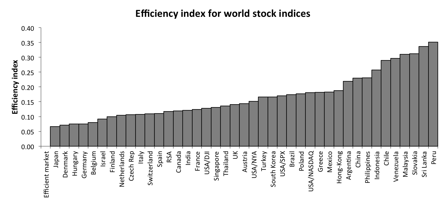
Figure 1: Efficiency index.

5 Results and discussion

We analyze efficiency of 41 stock market indices, which are described in Table 1. The dataset covers indices from the North and Latin America, Western Europe, Eastern Europe, Asia, Oceania and Africa and it has been obtained from dukascopy.com public database. The analyzed period ranges from the beginning of 2000 to the end of August 2011 (except of the indices which were founded later than 2000). The period thus includes each of the years of relatively stable growth, years of stable decrease after the DotCom bubble burst as well as the current crisis (crises). In Table 2, basic descriptive statistics of the logarithmic close/close returns are mentioned. Apart from the basic statistics (average, minimum, maximum, standard deviation, skewness and excess kurtosis), we show the KPSS statistics for the series. According to this test, all the series but CSE (Sri Lanka index) are weakly stationary. We do not show the results for ADF and PP unit-root tests since the test strongly rejects unit-root for all the indices with p-values practically equal to zero.

Let us now turn to the results. The results for efficiency index $EI$ are summarized in Fig. 1. In the figure, the indices are sorted so that the more to the left the index is, the more efficient it is. The most efficient market turns out to be the Japanese NIKKEI and the least efficient is the Peruvian IGRA. The ”Top 5” of the most efficient indices contains the Japanese NIKKEI, Danish KFX, Hungarian BUX, German DAX and Belgian BEL20. From the opposite side, the ”Bottom 5” includes Venezuelan IBC, Malaysian KLSE, Slovakian SAX, CSE of Sri Lanka and the already mentioned Peruvian IGRA. These are the results which might be labeled as relatively expected. However, when we look at the other indices, we can find more interesting results. First, the efficiency of the indices is geographically-dependent. For the more efficient half of the analyzed markets, there 13 European, 5 Asian, 2 North American and 1 African stock exchanges. The less efficient half contains 6 Latin American, 4 Asian, 4 European, 3 North American and 3 Oceanian. Therefore, the more efficient markets are dominated by European stock exchanges while the less efficient markets are dominated by Latin America, Asia and Oceania. Probably the most interesting are the performances of the US stock exchanges, which all score around the middle of the ranking. However, this should not be very surprising as the analyzed period contains both the DotCom bubble and the Global Financial Crisis of the late 2000s, which most severely hit the US markets and can be evidently taken as a source of inefficiency. Out of the four analyzed US indices, the most efficient turns out to be DJI and the least efficient is NASDAQ. Note that the most efficient US index, i.e. DJI, is less efficient than the biggest EU index – German DAX. British FTSE, which can be considered as tightly connected to the US indices ranks very similarly to the US indices, in the middle of the ranking. To be able to comment on the sources of inefficiency, we now focus on the separate measures.

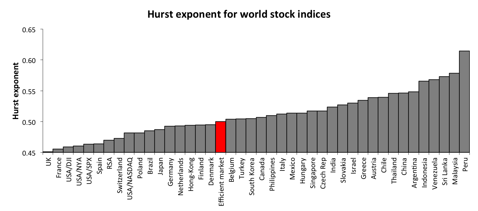
Figure 2: Hurst exponent.

Focusing on the Hurst exponent estimates, we observe that the deviations from the ideal $H=0.5$ are not that severe for majority of the indices and generally range between 0.45 and 0.55. In Fig. 2, we show the average values of the Hurst exponent estimates. Interestingly, we find that majority of the most developed markets (but not necessarily the most efficient as shown above) are below the $H=0.5$ level, which is in hand with the results of Di Matteo et al. [19]. Generally, we don’t observe strong global correlation structure in the processes. This is, however, not a big surprise as the existence of strong global auto-correlations would lead to arbitrage opportunities, which are not likely to last for long taking into account the computerized trading in the current markets. The indices with the highest Hurst exponents are the same as the least efficient markets. From these, the Peruvian IGRA shows higher persistence than the non-stationary CSE of Sri Lanka. Results for the first order autocorrelation are very similar for all indices and close to zero so that we do not present them.

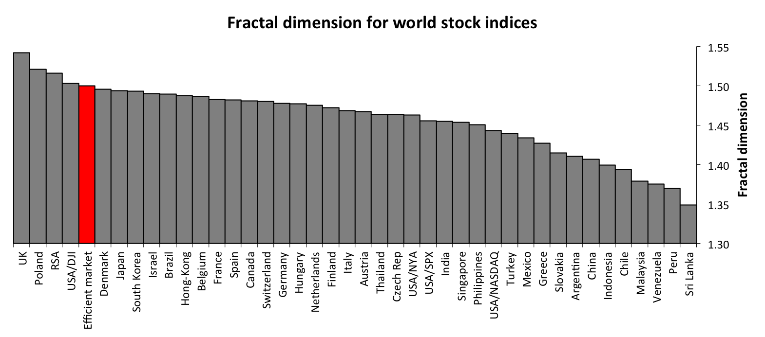
Figure 3: Fractal dimension.

The results for fractal dimension $D$ (Fig. 3) tell a more informative story. We observe that majority of the indices are characterized by the fractal dimension below 1.5, which indicates local persistence. For several indices, we observe the opposite. These are British FTSE, Polish WIG20, JSE of the Republic South Africa and DJI of the USA. Again the least efficient markets show the biggest deviation from $D=1.5$ and fall below 1.4. These markets thus experience relatively strong short-term trends and are at least partially predictable in the short term. Such a correlation structure even translates into global perspective as the markets with the lowest fractal dimension are also the markets with highest Hurst exponent. The general relationship between $H$ and $D$ for the analyzed indices is illustrated in Fig. 4. We observe that even though $D$ and $H$ are not independent, the relationship is not exactly of form $D=2-H$ of self-affine processes, yet it is very close to it. Specifically, the estimated relationship is $\widehat{D}=1.94-0.95\widehat{H}$ with $R^{2}=0.66$ which implies that fractal dimensions $D$ are paired with lower Hurst exponents $H$ than for the self-affine processes. This is exactly in hand with an economic interpretation that the local herding and crowd behavior are short-lasting and are thus not reflected in the global measure of the Hurst exponent $H$ perfectly but only partially. Such a result obviously makes sense in the stock markets where such a strong global dependence would lead to profitable opportunities which would vanish due to the interaction between supply and demand in the market. Nonetheless, the deviations of $D$ and $H$ from their efficient market values for the least efficient markets show that not only the profit opportunities are important for investors but also an institutional framework such as legal and regulation issues as well as liquidity issues. Otherwise, the profit opportunities even for the least efficient markets would vanish quickly.

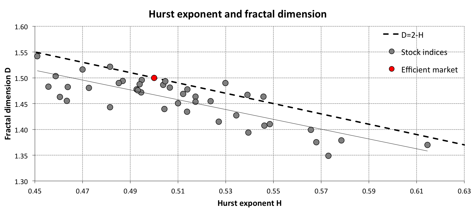
Figure 4: Relationship between Hurst exponent and fractal dimension.

To further illustrate different the effects of local and global inefficiencies into the total $EI$ measure, we present Fig. 5. We can see that for majority of indices, the local inefficiencies (deviation of the fractal dimension from 1.5) dominate the global inefficiencies (short-term and long-term memory). Interestingly for the least efficient markets, the dominance is the most evident. There are two exceptions for which the global inefficiencies dominate and these are Israeli TA100 and Austrian ATX. For the more efficient markets, the proportion of local inefficiencies is around 40% and for the less efficient markets, it is around 80% of the total.

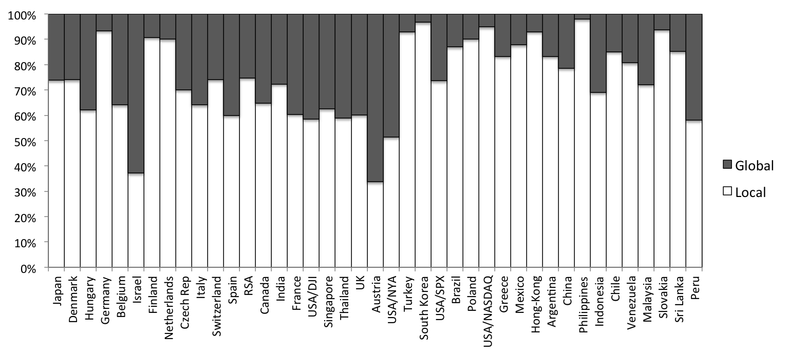
Figure 5: Separation between local and global inefficiencies from the most efficient market on the left to the least efficient market on the right.

6 Conclusions

We have introduced a novel approach to measuring capital market efficiency. With a use of bounded measures of dynamic systems connected to a standard martingale definition of the capital market efficiency, we constructed a vector containing long-term memory, short-term memory and fractal dimension measures. The efficiency index $EI$ is calculated as a simple norm of this vector from its ideal efficient case. Therefore, a distance of a specific market situation from a centre of an $n$-dimensional cube is taken as a measure of efficiency. The further the market is from the ideal state, the less efficient it is. Such procedure can be easily generalized to more bounded efficiency quantities.

Applying the methodology on a set of 41 stock indices in period between 2000 and 2011, we found that the Japanese NIKKEI is the most efficient market. From geographical point of view, the more efficient markets are dominated by European stock indices and the less efficient markets cover mainly the Latin America, Asia and Oceania. More specifically, the least efficient markets are Venezuelan IBC, Malaysian KLSE, Slovakian SAX, CSE of Sri Lanka and Peruvian IGRA (the most inefficient stock market in the analyzed set). We also found that the local characteristics of the series (crowd and herding behavior) partially translate into the global characteristics (correlation structure). Moreover, the local inefficiencies in general dominate the total inefficiency for strong majority of the indices.

References

References

- Alessio et al. [2002] Alessio, E., A. Carbone, G. Castelli, and V. Frappietro (2002). Second-order moving average and scaling of stochastic time series. European Physical Journal B 27, 197–200.
- Alexeev and Tapon [2011] Alexeev, V. and F. Tapon (2011). Testing weak form efficiency on the Toronto Stock Exchange. Journal of Empirical Finance 18, 661–691.
- Alvarez-Ramirez et al. [2002] Alvarez-Ramirez, J., M. Cisneros, C. Ibarra-Valdez, and A. Soriano (2002). Multifractal Hurst analysis of crude oil prices. Physica A 313, 651–670.
- Barabasi et al. [1991] Barabasi, A.-L., P. Szepfalusy, and T. Vicsek (1991). Multifractal spectre of multi-affine functions. Physica A 178, 17–28.
- Barkoulas and Baum [1996] Barkoulas, J. and C. Baum (1996). Long-term dependence in stock returns. Economics Letters 53, 253–259.
- Barunik et al. [2012] Barunik, J., T. Aste, T. Di Matteo, and R. Liu (2012). Understanding the source of multifractality in financial markets. Physica A 391, 4234–4251.
- Barunik and Kristoufek [2010] Barunik, J. and L. Kristoufek (2010). On Hurst exponent estimation under heavy-tailed distributions. Physica A 389(18), 3844–3855.
- Cajueiro and Tabak [2004a] Cajueiro, D. and B. Tabak (2004a). Evidence of long range dependence in Asian equity markets: the role of liquidity and market restrictions. Physica A 342, 656–664.
- Cajueiro and Tabak [2004b] Cajueiro, D. and B. Tabak (2004b). The Hurst exponent over time: testing the assertion that emerging markets are becoming more efficient. Physica A 336, 521–537.
- Cajueiro and Tabak [2004c] Cajueiro, D. and B. Tabak (2004c). Ranking efficiency for emerging markets. Chaos, Solitons and Fractals 22, 349–352.
- Cajueiro and Tabak [2005] Cajueiro, D. and B. Tabak (2005). Ranking efficiency for emerging equity markets II. Chaos, Solitons and Fractals 23, 671–675.
- Cajueiro and Tabak [2007] Cajueiro, D. and B. Tabak (2007). Long-range dependence and multifractality in the term structure of LIBOR interest rates. Physica A 373, 603–614.
- Carbone et al. [2004] Carbone, A., G. Castelli, and H. Stanley (2004). Time-dependent Hurst exponent in financial time series. Physica A 344, 267 271.
- Chan et al. [1996] Chan, G., P. Hall, and D. Poskitt (1996). Periodogram-based estimators of fractal properties. Annals of Statistics 23(5), 1684–1711.
- Charles et al. [2011] Charles, A., O. Darne, and J. Fouilloux (2011). Testing the martingale difference hypothesis in emission allowances. Economic Modelling 28, 27–35.
- Chong et al. [2011] Chong, T., T.-H. Lam, and I. Yan (2011). Is the Chinese stock market really inefficient? China Economic Review 23(1), 122 137.
- Di Matteo [2007] Di Matteo, T. (2007). Multi-scaling in finance. Quantitatice Finance 7(1), 21–36.
- Di Matteo et al. [2003] Di Matteo, T., T. Aste, and M. Dacorogna (2003). Scaling behaviors in differently developed markets. Physica A 324, 183–188.
- Di Matteo et al. [2005] Di Matteo, T., T. Aste, and M. Dacorogna (2005). Long-term memories of developed and emerging markets: Using the scaling analysis to characterize their stage of development. Journal of Banking & Finance 29, 827–851.
- Eom et al. [2008] Eom, C., G. Oh, and W.-S. Jung (2008). Relationship between efficiency and predictability in stock price change. Physica A 387, 5511–5517.
- Fama [1970] Fama, E. (1970). Efficient Capital Markets: A Review of Theory and Empirical Work. Journal of Finance 25, 383–417.
- Fama [1991] Fama, E. (1991). Efficient Capital Markets: II. Journal of Finance 46(5), 1575–1617.
- Genton [1998] Genton, M. (1998). Highly robust variogram estimation. Mathematical Geology 30, 213–221.
- Gneiting and Schlather [2004] Gneiting, T. and M. Schlather (2004). Stochastic Models That Separate Fractal Dimension and the Hurst Effect. SIAM Review 46(2), 269–282.
- Gneiting et al. [2010] Gneiting, T., H. Sevcikova, and D. Percival (2010). Estimators of fractal dimension: Assessing the roughness of time series and spatial data. Technical report, Department of Statistics, University of Washington.
- Hall and Wood [1993] Hall, P. and A. Wood (1993). On the performane of box-counting estimators of fractal dimension. Biometrika 80(1), 246–252.
- Hurst [1951] Hurst, H. (1951). Long term storage capacity of reservoirs. Transactions of the American Society of Engineers 116, 770–799.
- Kantelhardt et al. [2002] Kantelhardt, J., S. Zschiegner, E. Koscielny-Bunde, A. Bunde, S. Havlin, and E. Stanley (2002). Multifractal Detrended Fluctuation Analysis of Nonstationary Time Series. Physica A 316(1-4), 87–114.
- Kristoufek [2010a] Kristoufek, L. (2010a). On spurious anti-persistence in the US stock indices. Chaos, Solitons and Fractals 43, 68–78.
- Kristoufek [2010b] Kristoufek, L. (2010b). Rescaled range analysis and detrended fluctuation analysis: Finite sample properties and confidence intervals. AUCO Czech Economic Review 4, 236–250.
- Kristoufek [2012a] Kristoufek, L. (2012a). Fractal Markets Hypothesis and the Global Financial Crisis: Scaling, Investment Horizons and Liquidity. Advances in Complex Systems 15(6), 1250065.
- Kristoufek [2012b] Kristoufek, L. (2012b). How are rescaled range analyses affected by different memory and distributional properties? A Monte Carlo study. Physica A 391, 4252–4260.
- Lam and Tam [2011] Lam, K. and L. Tam (2011). Liquidity and asset pricing: Evidence from Hong Kong stock market. Journal of Banking & Finance 35, 2217–2230.
- Lim et al. [2008] Lim, K.-P., R. Brooks, and J. Kim (2008). Financial crisis and stock market efficiency: Empirical evidence from Asian countries. International Review of Financial Analysis 17, 571–591.
- Malkiel [2003] Malkiel, B. (2003). The efficient market hypothesis and its critics. Journal of Economic Perspectives 17(1), 59 82.
- Mandelbrot [1982] Mandelbrot, B. (1982). The fractal geometry of nature. W. H. Freeman Press.
- Mandelbrot and van Ness [1968] Mandelbrot, B. and J. van Ness (1968). Fractional Brownian motions, fractional noises and applications. SIAM Review 10(4), 422–437.
- Morales et al. [2012] Morales, R., T. Di Matteo, R. Gramatica, and T. Aste (2012). Dynamical generalized Hurst exponent as a tool to monitor unstable periods in financial series. Physica A 391, 3180–3189.
- Neves et al. [2011] Neves, L., F. Oliveira, F. Peres, R. Moreira, A. Moriel, M. de Godoy, and L. Murta Junior (2011). Maximum entropy, fractal dimension and lacunarity in quantification of cellular rejection in myocardial biopsy of patients submitted to heart transplantation. Journal of Physics: Conference Series 285, 012032.
- Panas [2001] Panas, E. (2001). Estimating fractal dimension using stable distributions and exploring long memory through ARFIMA models in Athens Stock Exchange. Applied Financial Economics 11, 395–402.
- Peng et al. [1993] Peng, C., S. Buldyrev, A. Goldberger, S. Havlin, M. Simons, and H. Stanley (1993). Finite-size effects on long-range correlations: Implications for analyzing DNA sequences. Physical Review E 47(5), 3730–3733.
- Peng et al. [1994] Peng, C., S. Buldyrev, S. Havlin, M. Simons, H. Stanley, and A. Goldberger (1994). Mosaic organization of DNA nucleotides. Physical Review E 49(2), 1685–1689.
- Percival and Walden [2000] Percival, D. and A. Walden (2000). Wavelet Methods for Time Series Analysis. Cambridge University Press.
- Podobnik et al. [2006] Podobnik, B., D. Fu, T. Jagric, I. Grosse, and H. E. Stanley (2006). Fractionally integrated process for transition economics. Physica A 362, 465–470.
- Vandewalle et al. [1997] Vandewalle, N., M. Ausloos, and P. Boveroux (1997). Detrended Fluctuation Analysis of the Foreign Exchange Market. In Econophysic Workshop, Budapest, Hungary.
- Weron [2002] Weron, R. (2002). Estimating long-range dependence: finite sample properties and confidence intervals. Physica A 312, 285 –299.
- Wright [2001] Wright, J. H. (2001). Long memory in emerging market stock returns. Emerging Markets Quarterly 5, 50–55.