Pair condensation in the BCS-BEC crossover
of ultracold atoms loaded onto a 2D square lattice

Abstract

We investigate the crossover from the Bardeen-Cooper-Schrieffer (BCS) state of weakly-bound Cooper pairs to the Bose-Einstein Condensate (BEC) of strongly-bound molecular dimers in a gas of ultracold atoms loaded on a two-dimensional optical lattice. By using the the mean-field BCS equations of the emerging Hubbard model and the concept of off-diagonal-long-range-order for fermions we calculate analytically and numerically the pair binding energy, the energy gap and the condensate fraction of Cooper pairs as a function of interaction strength and filling fractor of atoms in the lattice at zero temperature.

I Introduction

Several experimental groups greiner ; regal ; kinast ; zwierlein ; chin ; ueda have observed in ultracold alkali-metal atoms the predicted eagles ; leggett ; noziers crossover from the Bardeen-Cooper-Schrieffer (BCS) state of weakly bound Fermi pairs to the Bose-Einstein condensate (BEC) of molecular dimers. In two zwierlein ; ueda of these experiments the condensate fraction of Cooper pairs yang has been studied with two hyperfine component Fermi vapours of ⁶Li atoms. The experimental data of the condensate fraction, which is directly related to the off-diagonal-long-range order of the two-body density matrix of fermions penrose ; campbell , are in quite good agreement with mean-field theoretical predictions sala-odlro ; ortiz and Monte-Carlo simulations astrakharchik at zero temperature, while at finite temperature beyond-mean-field corrections are needed ohashi . Recently the condensate fraction in the BCS-BEC crossover has been theoretically investigated for a two-dimensional (2D) uniform Fermi gas sala-odlro2 , for a uniform three-spin-component Fermi gas with SU(3) symmetry sala-odlro3 , for a 2D uniform two-component Fermi gas with Rashba spin-orbit coupling sala-odlro4 ; cinesi , and also for neutron matter sala-odlro5 . Two years ago 2D degenerate Fermi gases have been experimentally realized for ultra-cold atoms in a highly anisotropic disk-shaped potential turlapov .

Motivated by these recent theoretical and experimental achievements, in the present paper we analyze the condensate fraction in the BCS-BEC crossover for a quasi-2D two-component Fermi gas under optical confinement, which gives rise to a two-dimensional square lattice stoof . In particular we study the energy gap and the condensate fraction of Cooper pairs as a function of the interaction strength (or equivalently as a function of binding energy of pairs) and filling factor of atoms in the lattice by using the concept of off-diagonal-long-range-order yang ; penrose ; campbell and solving the mean-field BCS equations stoof . The paper is organized as follows. In Section II we introduce the model Hamiltonian which describes two-spin-component Fermi atoms loaded onto a quasi-2D optical lattice. In Section III we discuss and solve the zero-temperature mean-field BCS equations as a function of the adimensional ratio between the interaction energy per site and the tunneling energy, calculating the binding energy of atomic pairs, the chemical potential and the energy gap order parameter. In particular, we compare the numerical results obtained by using the exact density of states with the analytical ones derived from an approximated density of states. In Section IV we calculate the condensate fraction of atomic pairs investigating the dependence of the condensate fraction on the relevant parameters of the system: scaled inter-atomic strength and filling factor. The paper is concluded by Section V.

II Fermi atoms on a quasi-2D lattice

The Hamiltonian of a confined dilute and ultracold gas of two-component Fermi atoms is given by

$${\hat{H}} = \int d^{3}{\bf r}\sum_{\sigma}{\hat{\psi}}_{\sigma}^{+}({\bf r})\left[-{\hbar^{2}\over 2m}\nabla^{2}+V_{ext}({\bf r})\right]{\hat{\psi}}_{\sigma}({\bf r})$$ (1)

$$+ g\int d^{3}{\bf r}\,{\hat{\psi}}_{\uparrow}^{+}({\bf r})\,{\hat{\psi}}^{+}_{\downarrow}({\bf r})\,{\hat{\psi}}_{\downarrow}({\bf r})\,{\hat{\psi}}_{\uparrow}({\bf r})\;,$$

where ${\hat{\psi}}_{\sigma}({\bf r})$ is the fermionic field operator that destroys an atom of pseudo-spin $\sigma$ ($\sigma=\uparrow,\downarrow$) at the position ${\bf r}$ and $g=4\pi\hbar^{2}a_{s}/m$ is the interaction strength of the contact inter-particle potential with $a_{s}$ the s-wave scattering length. The external optical potential

$$V_{ext}({\bf r})=V_{lat}(x,y)+{1\over 2}m\omega_{z}^{2}z^{2}$$ (2)

produces a harmonic confinement along the $z$ axis and a periodic potential

$$V_{lat}(x,y)=V_{0}\,\left(\cos^{2}{({2\pi\over\lambda}x)}+\cos^{2}{({2\pi\over\lambda}y)}\right)\;$$ (3)

in the $(x,y)$ plane, with $\lambda$ the wavelength of the laser light which determines the optical lattice stoof . The minima of the lattice potential form a two-dimensional square lattice with sites in the positions ${\bf R}_{\bf i}=a\,{\bf i}=a\,(i_{x},i_{y})$, where $a=\lambda/2$ is the lattice spacing and ${\bf i}=(i_{x},i_{y})$ is a 2D vector of integer numbers.

Using the set of Wannier functions in the lowest Bloch band stoof , where the Wannier function $W_{{\bf i}}(x,y)$ is maximally localized at site ${\bf R}_{\bf i}$, we can expand the fermionic field operator as:

$${\hat{\psi}}_{\sigma}({\bf r})=\sum_{\bf i}{\hat{c}}_{{\bf i}\sigma}\,W_{\bf i}(x,y)\,{e^{-z^{2}/(2a_{z}^{2})}\over\pi^{1/4}a_{z}^{1/2}}\;,$$ (4)

where ${\hat{c}}_{{\bf i}\sigma}$ and ${\hat{c}}_{{\bf i}\sigma}$ obey the usual Fermi anti-commutation relations, and $a_{z}=\sqrt{\hbar/(m\omega_{z})}$ is the characteristic length of the strong harmonic confinement along the $z$ axis, which induces a quasi-2D confinement if $\hbar\omega_{z}$ is much larger than the other energies of the system. Under these conditions, the Hamiltonian (1) can be written as

$${\hat{H}}=-t\sum_{\langle{\bf i}{\bf j}\rangle\,\sigma}{\hat{c}}^{+}_{{\bf i}\sigma}{\hat{c}}_{{\bf j}\sigma}+U\sum_{\bf i}{\hat{n}}_{{\bf i}\uparrow}{\hat{n}}_{{\bf i}\downarrow}\;,$$ (5)

where $\langle{\bf i}{\bf j}\rangle$ means nearest neighbor sites,

$$t=-\int dx\,dy\,W_{{\bf i}}^{*}(x,y)\left[-{\hbar^{2}\over 2m}\nabla^{2}+V_{latt}(x,y)\right]W_{{\bf j}}(x,y)$$ (6)

is the hopping parameter ($t>0$), i.e. the tunneling energy between nearest neighbor sites, and

$$U={g\over\pi a_{z}}\int dx\,dy\,|W_{{\bf i}}(x,y)|^{4}$$ (7)

is the on-site strength of the inter-atomic interaction. ${\hat{n}}_{{\bf i}\sigma}={\hat{c}}_{{\bf i}\sigma}^{+}{\hat{c}}_{{\bf i}\sigma}$ is the number operator which describes the number of atoms with spin $\sigma$ at the site ${\bf i}$, and consequently the total number operator reads

$${\hat{N}}=\sum_{{\bf i}\,\sigma}\,{\hat{n}}_{{\bf i}\sigma}\;.$$ (8)

Notice that Eq. (7) holds under the conditions $|a_{s}|\ll a_{z}$ and $|a_{s}|\ll a$, which ensure the absence of confinement induced resonance cir and no distorsion of Cooper pairs due to neighbor valleys of the optical confinement. In the Hubbard-like Hamiltonian (5) we have not included the tunneling energies between sites which are not nearest neighbor because they are exponentially suppressed. We have also assumed the on-site one-body energies to be the same on all sites and therfore dropped them as irrelevant stoof .

III Mean-field BCS equations

It is well known that the BCS state appears only in the case of an attractive strength, i.e. $U<0$ stoof . In the past the negative-$U$ Hubbard Hamiltonian has been investigated by various authors review as a model for high-$T_{c}$ superconductivity. More recently, it has been used to study the BCS-BEC crossover on 2D and 3D lattices both at zero andrenacci ; kujawa ; capone and finite temperature dupuis ; tamaki . As stressed in the introduction, motivated by recent theoretical and experimental achievement with ultracold atoms in optical lattices, here we reconsider the 2D negative-$U$ Hubbard Hamiltonian to investigate the pair condensation, and in particular the condensate fraction of Fermi atoms in the 2D lattice at zero temperature. Note that he condensate fraction has been calculated by Kujawa kujawa in the 3D square lattice with a generalized Hubbard model, but only in the special case $|U|/t=\infty$ . In the following sections we calculate, as a function of $|U|/t$ and of the filling factor, the energy gap and condensate fraction in the 2D square lattice, analyzing also the pair binding energy, which is always finite in the 2D BCS-BEC crossover.

We start by decoupling the interaction Hamiltonian of Eq. (5) in both normal and anomalous channels privitera

$${\hat{n}}_{{\bf i}\uparrow}{\hat{n}}_{{\bf i}\downarrow} \simeq \langle{\hat{n}}_{{\bf i}\uparrow}\rangle{\hat{n}}_{{\bf i}\downarrow}+{\hat{n}}_{{\bf i}\uparrow}\langle{\hat{n}}_{{\bf i}\downarrow}\rangle-\langle{\hat{c}}_{{\bf i}\uparrow}^{+}{\hat{c}}_{{\bf i}\downarrow}^{+}\rangle{\hat{c}}_{{\bf i}\uparrow}{\hat{c}}_{{\bf i}\downarrow}$$

$$- {\hat{c}}_{{\bf i}\uparrow}^{+}{\hat{c}}_{{\bf i}\downarrow}^{+}\langle{\hat{c}}_{{\bf i}\uparrow}{\hat{c}}_{{\bf i}\downarrow}\rangle-\langle{\hat{n}}_{{\bf i}\uparrow}\rangle\langle{\hat{n}}_{{\bf i}\downarrow}\rangle+\langle{\hat{c}}_{{\bf i}\uparrow}^{+}{\hat{c}}_{{\bf i}\downarrow}^{+}\rangle\langle{\hat{c}}_{{\bf i}\uparrow}{\hat{c}}_{{\bf i}\downarrow}\rangle\;.$$

We also assume

$${n\over 2}=\langle{\hat{n}}_{{\bf i}\uparrow}\rangle=\langle{\hat{n}}_{{\bf i}\uparrow}\rangle$$ (10)

and introduce the (real) mean-field, site-independent, gap order parameter

$$\Delta=-U\langle{\hat{c}}_{{\bf i}\uparrow}^{+}{\hat{c}}_{{\bf i}\downarrow}^{+}\rangle=-U\langle{\hat{c}}_{{\bf i}\downarrow}{\hat{c}}_{{\bf i}\uparrow}\rangle\;.$$ (11)

In this way we obtain the mean-field Hamiltonian

$${\hat{H}}_{MF} = -t\sum_{\langle{\bf i}{\bf j}\rangle\,\sigma}{\hat{c}}^{+}_{{\bf i}\sigma}{\hat{c}}_{{\bf j}\sigma}+{Un\over 2}\sum_{\bf i}\left({\hat{n}}_{{\bf i}\uparrow}+{\hat{n}}_{{\bf i}\downarrow}\right)$$

$$+ \Delta\sum_{\bf i}\left({\hat{c}}_{{\bf i}\uparrow}{\hat{c}}_{{\bf i}\downarrow}+{\hat{c}}_{{\bf i}\downarrow}^{+}{\hat{c}}_{{\bf i}\uparrow}^{+}\right)-{Un^{2}\over 4}N_{s}+{\Delta^{2}\over U}N_{s}\;,$$

where $N_{s}$ is the number of lattice sites.

In the dual space of wavevectors ${\bf k}=(k_{x},k_{y})$, setting

$${\hat{c}}_{{\bf i}\sigma}=\sum_{\bf k}{\hat{c}}_{{\bf k}\sigma}\ {e^{i{\bf k}\cdot{\bf R}_{\bf i}}\over\sqrt{N_{s}}}\;,$$ (13)

where ${\hat{c}}_{{\bf k}\sigma}$ destroys an atom of spin $\sigma$ and wavevector ${\bf k}$, the mean-field Hamiltonian (III) becomes

$${\hat{H}}_{MF} = \sum_{\bf k}\left(\epsilon_{\bf k}+{Un\over 2}\right){\hat{c}}_{{\bf k}\sigma}^{+}{\hat{c}}_{{\bf k}\sigma}$$

$$+ \Delta\sum_{{\bf k}}\left({\hat{c}}_{{\bf k}\uparrow}{\hat{c}}_{-{\bf k}\downarrow}+{\hat{c}}_{-{\bf k}\downarrow}^{+}{\hat{c}}_{{\bf k}\uparrow}^{+}\right)-{Un^{2}\over 4}N_{s}+{\Delta^{2}\over U}N_{s}\;,$$

where

$$\epsilon_{\bf k}=-2t\left(\cos{(k_{x}a)}+\cos{(k_{y}a)}\right)\;,$$ (15)

is the single-particle energy. We stress that we are considering only the lowest Bloch band. This single-band approximation for the BCS-BEC crossover is reliable since the crossover occours at magnetic fields that are relatively far away from the Feshbach resonance underlying it stoof2 . Moreover the approximation is reliable under the following conditions stoof2 ; georges : i) there are no more than two fermions per site; ii) the two lowest bands do not overlap, implying that $V_{0}\gg E_{r}$, which means $8t\ll E_{r}$, and $|U|\ll E_{g}$. $E_{r}=\hbar^{2}k_{L}^{2}/(2m)$ is the recoil energy with $k_{L}=2\pi/a$ the wavevector of the 2D optical lattice, and $E_{g}$ is the energy gap between the first and the second Bloch band.

We calculate the thermodynamic potential

$$\Omega=\langle{\hat{H}}_{MF}\rangle-\mu\,\langle\hat{N}\rangle\;,$$ (16)

where $\mu$ is the chemical potential which determines the average number $N=\langle{\hat{N}}\rangle$ of fermions, by introducing the Bogoliubov canonical transformation:

$${\hat{\alpha}}_{\bf k}=u_{\bf k}\,{\hat{c}}_{{\bf k}\uparrow}-v_{\bf k}\,{\hat{c}}_{-{\bf k}\downarrow}^{+}\;,\quad\quad{\hat{\beta}}_{\bf k}=u_{\bf k}\,{\hat{c}}_{-{\bf k}\downarrow}+v_{\bf k}\,{\hat{c}}_{{\bf k}\uparrow}^{+}\;,$$ (17)

where $u_{\bf k}$ and $v_{\bf k}$ are real and $u_{\bf k}^{2}+v_{\bf k}^{2}=1$. After the mimimization of $\Omega$ with respect to $\mu$ and $\Delta$ we recover the standard BCS equation stoof ; privitera for the average number of particles per site

$$n=2{1\over N_{s}}\sum_{\bf k}v_{\bf k}^{2}\;,$$ (18)

and the familiar BCS gap equation

$${1\over|U|}={1\over N_{s}}\sum_{\bf k}{1\over 2E_{\bf k}}\;,$$ (19)

where the quasi-particle amplitudes $u_{\bf k}$ and $v_{\bf k}$ are given by

$$v_{\bf k}^{2}={1\over 2}\left(1-\frac{\epsilon_{\bf k}-h}{E_{\bf k}}\right)\,,$$ (20)

and $u_{\bf k}^{2}=1-v_{\bf k}^{2}$. Here the Bogoliubov energy reads

$$E_{\bf k}=\left[\left(\epsilon_{\bf k}-h\right)^{2}+\Delta^{2}\right]^{1/2}$$ (21)

where

$$h=\mu-{Un\over 2}\;,$$ (22)

is the effective chemical potential which takes into account the Hartree interaction. The effective chemical potential $h$ and the gap energy $\Delta$ are obtained by solving equations (18) and (19). In the continuum limit $\sum_{\bf k}\to a^{2}N_{s}\int_{\cal BZ}d^{2}{\bf k}/(2\pi)^{2}$ and introducing the density of states (DOS) per site

$${\cal D}(\epsilon) = a^{2}\int_{\cal BZ}{d^{2}{\bf k}\over(2\pi)^{2}}\;\delta(\epsilon_{\bf k}-\epsilon)$$

$$= {1\over 2\pi^{2}t}K\left(\sqrt{1-{\epsilon^{2}\over 16t^{2}}}\right)\,\Theta\left(1-{\epsilon^{2}\over 16t^{2}}\right)\;,$$

where ${\cal BZ}=[-\pi/2,\pi/a]\times[-\pi/a,\pi/2]$ is the first Brillouin zone, $K(x)$ is the complete Elliptic integral of the first kind and $\Theta(x)$ is the step function, the number equation (18) and the gap equation (19) can be written as

$$n = \int_{-4t}^{4t}d\epsilon\,{\cal D}(\epsilon)\,\left(1-{\epsilon-h\over\sqrt{(\epsilon-h)^{2}+\Delta^{2}}}\right)\;,$$ (24)

$${1\over|U|} = \int_{-4t}^{4t}d\epsilon\,{\cal D}(\epsilon)\,{1\over 2\sqrt{(\epsilon-h)^{2}+\Delta^{2}}}\;.$$ (25)

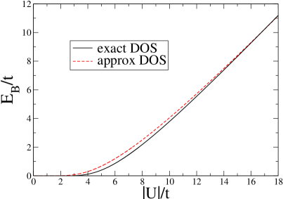
Figure 1: (Color online). Scaled binding energy $E_{B}/t$ as a function of the scaled interaction strength $|U|/t$, with $t$ the tunneling energy. Solid lines are the results obtained with the exact density of states (exact DOS) given by Eq. (III), while dashed lines are the results obtained with the approximate density of states (approx DOS) given by Eq. (27).

As discussed in review , quite generally in two dimensions a bound-state energy $E_{B}$ exists for any value of the negative interaction strength $U$. For the contact potential the bound-state equation in the lattice is

$${1\over|U|}=\int_{-4t}^{4t}d\epsilon\,{\cal D}(\epsilon)\,{1\over 2(\epsilon-\epsilon_{\bf 0})+E_{B}}\,,$$ (26)

where $\epsilon_{\bf 0}=-4t$ is the lower value of the single-particle energy $\epsilon_{\bf k}$, occurring at ${\bf k}={\bf 0}$. If we approximate the true DOS with a constant value in the interval $[-4t,4t]$, i.e.

$${\cal D}(\epsilon)\simeq{1\over 8t}\,\Theta\left(1-{\epsilon^{2}\over 16t^{2}}\right)\;,$$ (27)

that ensures the normalization

$$\int_{-4t}^{4t}d\epsilon\,{\cal D}(\epsilon)=1\,,$$ (28)

the bound-state equation can be solved analytically giving

$${1\over|U|}={1\over 16t}\ln{\left|{E_{B}+16t\over E_{B}}\right|}\;.$$ (29)

In Fig. 1 we plot the binding energy $E_{B}/t$ as a function of the interaction strength $|U|$ obtained with this approximate formula (dashed line). For comparison we plot also the exact result (solid line), obtained by numerically solving Eq. (26). The figure shows that the agreement between the two curves is extremely good. The BCS-BEC crossover is governed by the adimensional parameter $|U|/t$ or equivalently by the scaled binding energy $E_{B}/t$. The limit of large tunneling and small interaction $|U|/t\ll 1$ corresponds to the BCS regime where $E_{B}/t$ is close to zero. Instead the limit of strong localization and large interaction $|U|/t\gg 1$ corresponds to the BEC regime where $E_{B}/t$ is large.

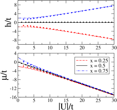
Figure 2: (Color online). Scaled effective chemical potential $h/t$ (upper panel) and scaled chemical potential $\mu/t$ (lower panel) as a function of the scaled interaction strength $|U|/t$, with $t$ the tunneling energy. Results obtained for three values of the filling factor $x=n/2$. Filled circles are the results obtained with the exact density of states given by Eq. (III), while lines are the results obtained with the approximate density of states given by Eq. (27).

The quite good agreement between the solid curve and the dashed curve of Fig. 1 suggests that one could use the approximate DOS to study various ground-state properties of the system in the BCS-BEC. Within the approximation of a constant DOS in the band, i.e. Eq. (27), the number density equation and the gap equation read

$$n = {1\over 8t}\Big{(}8t-\sqrt{(4t-h)^{2}+\Delta^{2}}$$

$$+ \sqrt{(4t+h)^{2}+\Delta^{2}}\Big{)}\;,$$

$${1\over|U|} = {1\over 16t}\,\ln{\left|{h+\sqrt{h^{2}+\Delta^{2}}\over h-8t+\sqrt{(h-8t)^{2}+\Delta^{2}}}\right|}\;.$$ (31)

It is then straightforward to plot (see Fig. 2) the effective chemical potential $h$ (upper panel) and the chemical potential $\mu$ (lower panel) as a function of the scaled interaction strength $|U|/t$, for different values of the filling factor $x=n/2$ ($0\leq x\leq 1$). In the figure the lines are obtained by using Eqs. (III) and (III) based on the approximate DOS of Eq. (27), while the filled circles are obtained by using Eqs. (24) and (25) with the exact DOS of Eq. (III).

Fig. 2 shows that at half filling ($x=0.5$) the effective chemical potential $h$ remains always constant and equal to zero, and the corresponding chemical potential $\mu$ follows the simple law $\mu=-|U|/2$. Moreover, the lower panel of Fig. 2 shows that, at fixed filling factor $x$, the chemical potential $\mu$ as a function of $U$ is close to a straight line (it is true straight line only for $x=0.5$) and approaches $\mu\simeq-|U|/2$ for large $|U|$.

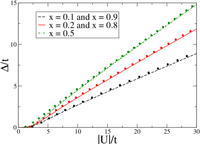
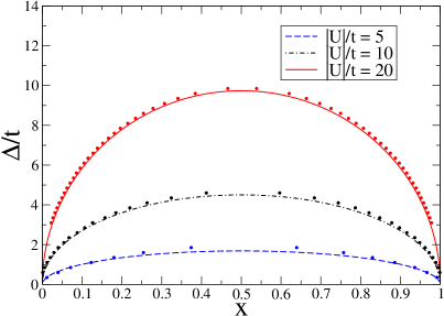
Figure 3: (Color online). Upper panel: Scaled energy gap $\Delta/t$ as a function of scaled interaction strength $|U|/t$ with $t$ the tunneling energy. The three curves correspond to five different values of the filling factor $x=n/2$. Lower panel: Scaled energy gap $\Delta/t$ as a function of filling factor $x=n/2$, where the three curves correspond to three different values of the scaled interaction strength $|U|/t$, with $t$ the tunneling energy. Filled circles are the results obtained with the exact density of states given by Eq. (III), while lines are the results obtained with the approximate density of states given by Eq. (27).

In Fig. 3 we plot the energy gap $\Delta$ vs interaction strength $|U|$ (upper panel) and vs filling factor $x$ (lower panel). The upper panel shows that, at fixed filling factor $x$, the energy gap $\Delta$ grows by increasing the scaled interaction strength $|U|/t$, that is by increasing the localization. Instead, the lower panel shows that, at fixed scaled interaction strength $|U|/t$, the scaled energy gap $\Delta/t$ reaches its maximum value at half filling $x=1/2$, i.e. when on the average there is one atom per site. This effect is clearly seen in the lower panel of Fig. 3 where we consider three values of $|U|/t$. Notice that the behavior of $\Delta$ as a function of $x$ is perfectly symmetric with respect to $x=1/2$ (half filling). Also in Fig. 3 the agreement between the results obtained with the exact DOS and the ones calculated with the approximate DOS is quite good, and it improves by increasing $|U|/t$. Motivated by this finding, in the remaining part of the paper we use the approximate DOS, which is much simpler for numerical computations and produces analytical results.

IV Condensate fraction

The main task of the paper is to analyze the condensate fraction of fermions. As shown by Yang yang , the BCS state guarantees the off-diagonal-long-range-order penrose of the Fermi gas, namely that, in the limit wherein both unprimed coordinates approach an infinite distance from the primed coordinates, the two-body density matrix factorizes as follows:

$$\langle{\hat{\psi}}^{+}_{\uparrow}({\bf r}_{1}^{\prime}){\hat{\psi}}^{+}_{\downarrow}({\bf r}_{2}^{\prime}){\hat{\psi}}_{\downarrow}({\bf r}_{1}){\hat{\psi}}_{\uparrow}({\bf r}_{2})\rangle$$ (32)

$$=\langle{\hat{\psi}}^{+}_{\uparrow}({\bf r}_{1}^{\prime}){\hat{\psi}}^{+}_{\downarrow}({\bf r}_{2}^{\prime})\rangle\langle{\hat{\psi}}_{\downarrow}({\bf r}_{1}){\hat{\psi}}_{\uparrow}({\bf r}_{2})\rangle\,.$$

The largest eigenvalue of the two-body density matrix (32) gives the number of pairs in the lowest two-particle state, i.e. the condensate number of Fermi pairs leggett ; yang ; campbell . In this way, the number $N_{0}$ of condensed fermions is given by

$$N_{0}=2\int d^{3}{\bf r}\,d^{3}{\bf r}^{\prime}\;|\langle{\hat{\psi}}_{\downarrow}({\bf r}){\hat{\psi}}_{\uparrow}({\bf r}^{\prime})\rangle|^{2}=2\sum_{{\bf i}{\bf j}}\;|\langle{\hat{c}}_{{\bf i}\downarrow}{\hat{c}}_{{\bf j}\uparrow}\rangle|^{2}.$$ (33)

Notice that, as said above, $N_{0}$ counts the number of condensed fermions: $0\leq N_{0}\leq N$ sala-odlro3 and not of condensed pairs. It is then quite easy to show that the the condensate number of atoms per site is

$$n_{0}=2{1\over N_{s}}\sum_{\bf k}u_{\bf k}^{2}v_{\bf k}^{2}\;.$$ (34)

With the help of Eqs. (20) this number is thus given by :

$$n_{0}={\Delta^{2}\over 2}\int_{-4t}^{4t}d\epsilon\,{\cal D}(\epsilon)\,{1\over(\epsilon-h)^{2}+\Delta^{2}}\;,$$ (35)

and using the approximate DOS of Eq. (27) it reads:

$$n_{0}={\Delta\over 16t}\left(\arctan{\left({4t-h\over\Delta}\right)}+\arctan{\left({4t+h\over\Delta}\right)}\right)\;.$$ (36)

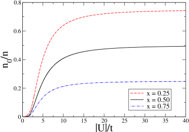
Figure 4: (Color online). Condensate fraction $n_{0}/n$ as a function of scaled interaction strength $|U|/t$ with $t$ the tunneling energy. The three curves correspond to three different values of the filling factor $x=n/2$.

Fig. 4 shows the condensate fraction $n_{0}/n$ of fermions, calculated with Eqs. (III), (31) and (36), as a function of scaled interaction strength $|U|/t$ for three values of the filling factor $x$. We have verified that the plotted results are in good agreement with the ones obtained by using the exact DOS, except in the case of very small values of $|U|/t$. In any case, the condensate fraction $n_{0}/n$ vanishes when the scaled interaction strength $|U|/t$ goes to zero. Moreover, as shown in the figure, the condensed fraction grows very fast for values of the scaled interaction strength $|U|/t\leq 8$, it shows a shoulder, and then it reaches its asymptotic value $n_{0}/n\simeq 1-x$ rather slowly.

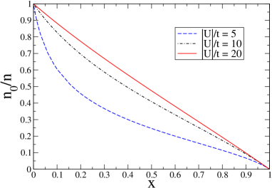
Figure 5: (Color online). Upper panel: Condensate fraction $n_{0}/n$ as a function of the filling factor $x=n/2$. Lower panel: Number $n_{0}$ of condensed atoms per site. The curves correspond to three different values of the scaled interaction strength $|U|/t$, with $t$ the tunneling energy.

This result is confirmed in the upper panel of Fig. 5, where we report the condensate fraction $n_{0}/n$ as a function of the filling factor $x$ at fixed scaled interaction strength $|U|/t$. The figure clearly shows that $n_{0}/n$ ranges from one to zero, being extremely close to one for $x\ll 1$ and approaching zero as $x$ goes to $1$. This means that there is a full BEC-BCS crossover by increasing $x$ at constant scaled interaction strength $|U|/t$. Moreover, if the scaled interaction strength $|U|/t$ is large, the condensate fraction $n_{o}/n$ follows a straight line during the BEC-BCS crossover. For the sake of completeness, in the lower panel of Fig. 5 we plot also the number $n_{0}$ of condensed atoms per site as a function of the filling factor $x$. The results show that the curves of $n_{o}$ vs $x$ have a behavior similar to those of $\Delta$ vs $x$ (see Fig. 3). In the limit $|U|/t\to\infty$ one finds that $n_{0}=(1-x)2x$ and consequently $n_{0}/n=(1-x)$.

Finally, we observe that, after a simple rescaling of the chemical potential, namely ${\tilde{h}}=h+4t$, in the limit $t\to\infty$ with $ta^{2}\to\pi\hbar^{2}/m$, Eq. (36) becomes the condensate number equation found in Ref. sala-odlro2 for the 2D uniform superfluid Fermi gas.

V Conclusions

By using the mean-field extended BCS theory and the concept of off-diagonal long-range order, that is the existence of a macroscopic eigenvalue of the two-body density matrix, we have investigated the condensate fraction of fermionic pairs in a uniform 2D Fermi gas. We have shown that the condensate number $n_{0}$ of fermi atoms per site is extremely useful to characterize the BCS-BEC crossover, that is induced by changing the adimensional ratio $|U|/t$ between the interaction energy $|U|$ and the tunneling energy $t$. In particular, we have found that both the scaled binding energy $E_{B}/t$ of atomic pairs and the condensate fraction $n_{0}/n$ grow by increasing the ratio $|U|/t$ at fixed filling factor $x=n/2$ (with $n$ the average number of fermions per site). In addition, our results suggest that fixing the ratio $|U|/t$, or equivalently the scaled binding energy $E_{B}/t$, there is a full BEC-BCS crossover by increasing the filling factor from zero to one. Finally, we have found that the analytical results obtained by using an approximate density of states are in quite good agreement with the numerical ones deduced from the exact density of states. In our calculations we have used the mean-field theory and it is important to stress that recent Monte Carlo simulations have shown that, at zero-temperature, beyond-mean-field effects are negligible in the BCS side of the BCS-BEC crossover while they become relevant in the deep BEC side astrakharchik ; bertaina . In any case, we think that our mean-field results, and the reliable analytical formulas we have obtained, can be of interest for near future experiments with degenerate gases made of alkali-metal atoms confined in quasi-2D optical lattices.

In this paper we have investigated zero-temperature pair condensation. According to the Mermin-Wagner theorem stoof , for an infinite 2D system there is condensation (off-diagonal-long-range order) only at zero temperature. However, for a finite 2D system condensation could be possible also at non-zero temperature. The investigation of this issue, which requires a beyond mean-field approach, for 2D fermions in a lattice is in progress. Another puzzling issue is the filling of the second Bloch band: we plan to investigate its effect on pair condensation by analyzing a multi-band version of the present theory.

References

- (1) M. Greiner, C.A. Regal, and D.S. Jin, Nature (London) 426, 537 (2003).
- (2) C.A. Regal, M. Greiner, and D.S. Jin, Phys. Rev. Lett. 92, 040403 (2004).
- (3) J. Kinast, S.L. Hemmer, M.E. Gehm, A. Turlapov, J.E. Thomas, Phys. Rev. Lett. 92, 150402 (2004).
- (4) M.W. Zwierlein et al., Phys. Rev. Lett. 92, 120403 (2004); M.W. Zwierlein, C.H. Schunck, C.A. Stan, S.M.F. Raupach, W. Ketterle, Phys. Rev. Lett. 94, 180401 (2005).
- (5) C. Chin et al., Science 305, 1128 (2004); M. Bartenstein et al., Phys. Rev. Lett. 92, 203201 (2004).
- (6) Y. Inada, M. Horikoshi, S. Nakajima, M. Kuwata-Gonokami, M. Ueda, and T. Mukaiyama, Phys. Rev. Lett. 101, 180406 (2008).
- (7) D.M. Eagles, Phys. Rev. 186, 456 (1969).
- (8) A.J. Leggett, in Modern Trends in the Theory of Condensed Matter, p. 13, edited by A. Pekalski and J. Przystawa (Springer, Berlin, 1980).
- (9) P. Noziers, S. Schmitt-Rink, J. Low Temp. Phys. 59, 195 (1985).
- (10) C.N. Yang, Rev. Mod. Phys. 34, 694 (1962).
- (11) O. Penrose, Phil. Mag. 42, 1373 (1951); O. Penrose and L. Onsager, Phys. Rev. 104, 576 (1956).
- (12) C.E. Campbell, in Condensed Matter Theories, vol. 12, 131 (Nova Science, New York, 1997).
- (13) L. Salasnich, N. Manini, and A. Parola, Phys. Rev. A 72, 023621 (2005).
- (14) G. Ortiz and J. Dukelsky, Phys. Rev. A 72, 043611 (2005).
- (15) G. E. Astrakharchik, J. Boronat, J. Casulleras, and S. Giorgini, Phys. Rev. Lett. 93, 200404 (2004).
- (16) Y. Ohashi and A. Griffin, Phys. Rev. A 72, 063606 (2005); N. Fukushima, Y. Ohashi, E. Taylor, and A. Griffin, Phys. Rev. A 75, 033609 (2007).
- (17) L. Salasnich, Phys. Rev. A 76, 015601 (2007).
- (18) L. Salasnich, Phys. Rev. A 83, 033630 (2011).
- (19) L. Dell’Anna, G. Mazzarella, and L. Salasnich, Phys. Rev. A 84, 033633 (2011).
- (20) J. Zhou, W. Zhang, and W. Yi, Phys. Rev. A 84, 063603 (2011); L. Jiang, X-J. Liu, H. Hu, and H. Pu, Phys. Rev. A 84, 063618 (2011); G. Chen, M. Gong, and C. Zhang, Phys. Rev. A 85 013601 (2012); K. Zhou and Z. Zhang, Phys. Rev. Lett. 108, 025301 (2012); L. He and X-G. Huang, Phys. Rev. Lett. 108, 145302 (2012).
- (21) L. Salasnich, Phys. Rev. C 84, 067301 (2011).
- (22) K. Martiyanov, V. Makhalov, and A. Turlapov, Phys. Rev. Lett. 105, 030404 (2010).
- (23) E. Haller, M.J. Mark, R. Hart, J.G. Danzl, L. Reichsöllner, V. Melezhik, P. Schmelcher, and H-C. Nägerl, Phys. Rev. Lett. 104, 153203 (2010).
- (24) H.T.C. Stoof, B.M. Dennis, and K. Gubbels, Ultracold Quantum Fields (Springer, Berlin, 2009).
- (25) For a review, see R. Micnas, J. Ranninger, and S. Robaszkiewicz, Rev. Mod. Phys. 62, 113 (1990).
- (26) N. Andrenacci, A. Perali, P. Pieri, and C.G. Strinati, Phys. Rev. B 60, 12410 (1999).
- (27) A. Kujawa, Acta Phys. Pol. A 111, 745 (2007).
- (28) A. Privitera and M. Capone, Phys. Rev. A 85, 013640 (2012).
- (29) N. Dupuis, Phys. Rev. B 70, 134502 (2004).
- (30) H. Tamaki, Y. Ohashi, and K. Miyake, Phys. Rev. A 77, 063616 (2008).
- (31) A. Privitera, Lattice Approach to the BCS-BEC Crossover in Dilute Systems: a MF and DMFT Approach, Ph.D. Thesis (Universitá “La Sapienza” di Roma, Rome, 2008).
- (32) A. Koetsier, D.B.M. Dickerscheid, and H.T.C. Stoof, Phys. Rev. A 74, 033621 (2006).
- (33) A. Georges, in Ultra-cold Fermi gases, Proceedings of the International School of Physics “Enrico Fermi”, vol. 164, edited by M. Inguscio, W. Ketterle and C. Salomon IOS Press, Amsterdam, 2008); arXiv:cond-mat/0702122.
- (34) G. Bertaina and S. Giorgini, Phys. Rev. Lett. 106, 110403 (2011).