Payment Rules through Discriminant-Based Classifiers

Abstract

In mechanism design it is typical to impose incentive compatibility and then derive an optimal mechanism subject to this constraint. By replacing the incentive compatibility requirement with the goal of minimizing expected ex post regret, we are able to adapt statistical machine learning techniques to the design of payment rules. This computational approach to mechanism design is applicable to domains with multi-dimensional types and situations where computational efficiency is a concern. Specifically, given an outcome rule and access to a type distribution, we train a support vector machine with a special discriminant function structure such that it implicitly establishes a payment rule with desirable incentive properties. We discuss applications to a multi-minded combinatorial auction with a greedy winner-determination algorithm and to an assignment problem with egalitarian outcome rule. Experimental results demonstrate both that the construction produces payment rules with low ex post regret, and that penalizing classification errors is effective in preventing failures of ex post individual rationality.

1 Introduction

Mechanism design studies situations where a set of agents each hold private information about their preferences over different outcomes. The designer chooses a center that receives claims about such preferences, selects and enforces an outcome, and optionally collects payments. The classical approach is to impose incentive compatibility, ensuring that agents truthfully report their preferences in strategic equilibrium. Subject to this constraint, the goal is to identify a mechanism, i.e., a way of choosing an outcome and payments based on agents’ reports, that optimizes a given design objective like social welfare, revenue, or some notion of fairness.

There are, however, significant challenges associated with this classical approach. First of all, it can be analytically cumbersome to derive optimal mechanisms for domains that are “multi-dimensional” in the sense that each agent’s private information is described through more than a single number, and few results are known in this case. Second, incentive compatibility can be costly, in that adopting it as a hard constraint can preclude mechanisms with useful economic properties. For example, imposing the strongest form of incentive compatibility, truthfulness in a dominant strategy equilibrium or strategyproofness, necessarily leads to poor revenue, vulnerability to collusion, and vulnerability to false-name bidding in combinatorial auctions where valuations exhibit complementarities among items [2, 21]. A third difficulty occurs when the optimal mechanism has an outcome or payment rule that is computationally intractable.

In the face of these difficulties, we adopt statistical machine learning to automatically infer mechanisms with good incentive properties. Rather than imposing incentive compatibility as a hard constraint, we start from a given outcome rule and use machine learning techniques to identify a payment rule that minimizes agents’ expected ex post regret relative to this outcome rule. Here, the ex post regret an agent has for truthful reporting in a given instance is the amount by which its utility could be increased through a misreport. While a mechanism with zero ex post regret for all inputs is obviously strategyproof, we are not aware of any additional direct implication in terms of equilibrium properties. Support for expected ex post regret as a quantifiable target for mechanism design rather comes from a simple model of manipulation where agents face a certain cost for strategic behavior. If this cost is higher than the expected gain, agents can be assumed to behave truthfully. We do insist on mechanisms in which the price to an agent, conditioned on an outcome, is independent of its report. This provides additional robustness against manipulation in the sense that there is no local price sensitivity.

Our approach is applicable to domains that are multi-dimensional or for which the computational efficiency of outcome rules is a concern. Given the implied relaxation of incentive compatibility, the intended application is to domains in which incentive compatibility is unavailable or undesirable for outcome rules that meet certain economic and computational desiderata. The payment rule is learned on the basis of a given outcome rule, and as such the framework is most meaningful in domains where revenue considerations are secondary to outcome considerations.

The essential insight is that the payment rule of a strategyproof mechanism can be thought of as a classifier for predicting the outcome: the payment rule implies a price to each agent for each outcome, and the selected outcome must be one that simultaneously maximizes reported value minus price for every agent. By limiting classifiers to discriminant functions with this “value-minus-price” structure, where the price can be an arbitrary function of the outcome and the reports of other agents, we obtain a remarkably direct connection between multi-class classification and mechanism design. For an appropriate loss function, the discriminant function of a classifier that minimizes generalization error over a hypothesis class has a corresponding payment rule that minimizes expected ex post regret among all payment rules corresponding to classifiers in this class. Conveniently, an appropriate method exists for multi-class classification with large outcome spaces that supports the specific structure of the discriminant function, namely the method of structural support vector machines [24, 12]. Just like standard support vector machines, it allows us to adopt non-linear kernels, thus enabling price functions that depend in a non-linear way on the outcome and on the reported types of other agents.

In illustrating the framework, we focus on two situations where strategyproof payment rules are not available: a greedy outcome rule for a multi-minded combinatorial auction in which each agent is interested in a constant number of bundles, and an assignment problem with an egalitarian outcome rule, i.e., an outcome rule that maximizes the minimum value of any agent. The experimental results we obtain are encouraging, in that they demonstrate low expected ex post regret even when the $0/1$ classification accuracy is only moderately good, and in particular better regret properties than those obtained through simple VCG-based payment rules that we adopt as a baseline. In addition, we give special consideration to the failure of ex post individual rationality, and introduce methods to bias the classifier to avoid these kinds of errors as well as post hoc adjustments that eliminate them. As far as scalability is concerned, we emphasize that the computational cost associated with our approach occurs offline during training. The learned payment rules have a succinct description and can be evaluated quickly in a deployed mechanism.

Related Work

Conitzer and Sandholm [6] introduced the agenda of automated mechanism design (AMD), which formulates mechanism design as an optimization problem. The output is the description of a mechanism, i.e., an explicit mapping from types to outcomes and payments. AMD is intractable in general, as the type space can be exponential in both the number of agents and the number of items, but progress has recently been made in finding approximate solutions for domains with additive value structure and symmetry assumptions, and adopting Bayes-Nash incentive compatibility (BIC) as the goal [4]. Another approach is to search through a parameterized space of incentive-compatible mechanisms [9].

A parallel literature allows outcome rules to be represented by algorithms, like our work, and thus extends to richer domains. Lavi and Swamy [15] employ LP relaxation to obtain mechanisms satisfying BIC for set-packing problems, achieving worst-case approximation guarantees for combinatorial auctions. Hartline and Lucier [10] and Hartline et al. [11] propose a general approach, applicable to both single-parameter and multi-parameter domains, for converting any approximation algorithm into a mechanism satisfying BIC that has essentially the same approximation factor with respect to social welfare. This approach differs from ours in that it adopts BIC as a target rather than the minimization of expected ex post regret. In addition, it evaluates the outcome rule on a number of randomly perturbed replicas of the instance that is polynomial in the size of a discrete type space, which is infeasible for combinatorial auctions where this size is exponential in the number of items. The computational requirements of our trained rule are equivalent to that of the original outcome rule.

Lahaie [13, 14] also adopts a kernel-based approach for combinatorial auctions, but focuses not on learning a payment rule for a given outcome rule but rather on solving the winner determination and pricing problem for a given instance of a combinatorial auction. Lahaie introduces the use of kernel methods to compactly represent non-linear price functions, which is also present in our work, but obtains incentive properties more indirectly through a connection between regularization and price sensitivity.

2 Preliminaries

A mechanism design problem is given by a set $N=\{1,2,\dots,n\}$ of agents that interact to select an element from a set $\Omega\subseteq\vartimes_{i\in N}\Omega_{i}$ of outcomes, where $\Omega_{i}$ denotes the set of possible outcomes for agent $i\in N$. Agent $i\in N$ is associated with a type $\theta_{i}$ from a set $\Theta_{i}$ of possible types, corresponding to the private information available to this agent. We write $\theta=(\theta_{1},\dots,\theta_{n})$ for a profile of types for the different agents, $\Theta=\vartimes_{i\in N}\Theta_{i}$ for the set of possible type profiles, and $\theta_{-i}\in\Theta_{-i}$ for a profile of types for all agents but $i$. Each agent $i\in N$ is further assumed to employ preferences over $\Omega_{i}$, represented by a valuation function $v_{i}:\Theta_{i}\times\Omega_{i}\rightarrow\mathbb{R}$. We assume that for all $i\in N$ and $\theta_{i}\in\Theta_{i}$ there exists an outcome $o\in\Omega$ with $v_{i}(\theta_{i},o_{i})=0$.

A (direct) mechanism is a pair $(g,p)$ of an outcome rule $g:\Theta\rightarrow\vartimes_{i\in N}\Omega_{i}$ and a payment rule $p:\Theta\rightarrow\mathbb{R}^{n}_{\geq 0}$. The intuition is that the agents reveal to the mechanism a type profile $\theta\in\Theta$, possibly different from their true types, and the mechanism chooses outcome $g(\theta)$ and charges each agent $i$ a payment of $p_{i}(\theta)=(p(\theta))_{i}$. We assume quasi-linear preferences, so the utility of agent $i$ with type $\theta_{i}\in\Theta_{i}$ given a profile $\theta^{\prime}\in\Theta$ of revealed types is $u_{i}(\theta^{\prime},\theta_{i})=v_{i}(\theta_{i},g_{i}(\theta^{\prime}))-p_{i}(\theta^{\prime})$, where $g_{i}(\theta)=(g(\theta)_{i})$ denotes the outcome for agent $i$. A crucial property of mechanism $(g,p)$ is that its outcome rule is feasible, i.e., that $g(\theta)\in\Omega$ for all $\theta\in\Theta$.

Outcome rule $g$ satisfies consumer sovereignty if for all $i\in N$, $o_{i}\in\Omega_{i}$, and $\theta^{\prime}_{-i}\in\Theta_{-i}$, there exists $\theta^{\prime}_{i}\in\Theta_{i}$ such that $g_{i}(\theta^{\prime}_{i},\theta^{\prime}_{-i})=o_{i}$; and reachability of the null outcome if for all $i\in N$, $\theta_{i}\in\Theta_{i}$, and $\theta^{\prime}_{-i}\in\Theta_{-i}$, there exists $\theta^{\prime}_{i}\in\Theta_{i}$ such that $v_{i}(\theta_{i},g_{i}(\theta^{\prime}_{i},\theta^{\prime}_{-i}))=0$.

Mechanism $(g,p)$ is dominant strategy incentive compatible, or strategyproof, if each agent maximizes its utility by reporting its true type, irrespective of the reports of the other agents, i.e., if for all $i\in N$, $\theta_{i}\in\Theta_{i}$, and $\theta^{\prime}=(\theta^{\prime}_{i},\theta^{\prime}_{-i})\in\Theta$, $u_{i}((\theta_{i},\theta^{\prime}_{-i}),\theta_{i})\geq u_{i}((\theta^{\prime}_{i},\theta^{\prime}_{-i}),\theta_{i})$; it satisfies individual rationality (IR) if agents reporting their true types are guaranteed non-negative utility, i.e., if for all $i\in N$, $\theta_{i}\in\Theta_{i}$, and $\theta^{\prime}_{-i}\in\Theta_{-i}$, $u_{i}((\theta_{i},\theta^{\prime}_{-i}),\theta_{i})\geq 0$. Observe that given reachability of the null outcome, strategyproofness implies individual rationality.

It is known that a mechanism $(g,p)$ is strategyproof if and only if the payment of an agent is independent of its reported type and the chosen outcome simultaneously maximizes the utility of all agents, i.e., if for every $\theta\in\Theta$,

$$p_{i}(\theta) =t_{i}(\theta_{-i},g_{i}(\theta)) \text{for all}\ i\in N,\ \text{and}$$ (1)

$$g_{i}(\theta) \in\arg\max_{\mathchoice{\hbox to0.0pt{\hss$\displaystyle{o^{\prime}_{i}\in\Omega_{i}}$\hss}}{\hbox to0.0pt{\hss$\textstyle{o^{\prime}_{i}\in\Omega_{i}}$\hss}}{\hbox to0.0pt{\hss$\scriptstyle{o^{\prime}_{i}\in\Omega_{i}}$\hss}}{\hbox to0.0pt{\hss$\scriptscriptstyle{o^{\prime}_{i}\in\Omega_{i}}$\hss}}}\bigl{(}v_{i}(\theta_{i},o^{\prime}_{i})-t_{i}(\theta_{-i},o_{i}^{\prime})\bigr{)} \text{for all}\ i\in N,$$ (2)

for a price function $t_{i}:\Theta_{-i}\times\Omega_{i}\rightarrow\mathbb{R}$. This simple characterization is crucial for the main results in the present paper, providing the basis with which the discriminant function of a classifier can be used to induce a payment rule.

In addition, a direct characterization of strategyproofness in terms of monotonicity properties of outcome rules explains which outcome rules can be associated with a payment rule in order to be “implementable” within a strategyproof mechanism [22, 1]. These monotonicity properties provide a fundamental constraint on when our machine learning framework can hope to identify a payment rule that provides full strategyproofness.

We quantify the degree of strategyproofness of a mechanism in terms of the regret experienced by an agent when revealing its true type, i.e., the potential gain in utility by revealing a different type instead. Formally, the ex post regret of agent $i\in N$ in mechanism $(g,p)$, given true type $\theta_{i}\in\Theta_{i}$ and reported types $\theta^{\prime}_{-i}\in\Theta_{-i}$ of the other agents, is

$$\mathit{rgt}_{i}(\theta_{i},\theta^{\prime}_{-i})=\max_{\mathchoice{\hbox to0.0pt{\hss$\displaystyle{\theta^{\prime}_{i}\in\Theta_{i}}$\hss}}{\hbox to0.0pt{\hss$\textstyle{\theta^{\prime}_{i}\in\Theta_{i}}$\hss}}{\hbox to0.0pt{\hss$\scriptstyle{\theta^{\prime}_{i}\in\Theta_{i}}$\hss}}{\hbox to0.0pt{\hss$\scriptscriptstyle{\theta^{\prime}_{i}\in\Theta_{i}}$\hss}}}u_{i}\bigl{(}(\theta^{\prime}_{i},\theta^{\prime}_{-i}),\theta_{i}\bigr{)}-u_{i}\bigl{(}(\theta_{i},\theta^{\prime}_{-i}),\theta_{i}\bigr{)}.$$

Analogously, the ex post violation of individual rationality of agent $i\in N$ in mechanism $(g,p)$, given true type $\theta_{i}\in\Theta_{i}$ and reported types $\theta^{\prime}_{-i}\in\Theta_{-i}$ of the other agents, is

$$\mathit{irv}_{i}(\theta_{i},\theta^{\prime}_{-i})=|\min(u_{i}((\theta_{i},\theta^{\prime}_{-i}),\theta_{i}),0)|.$$

We consider situations where types are drawn from a distribution with probability density function $D:\Theta\rightarrow\mathbb{R}$ such that $D(\theta)\geq 0$ and $\int_{\theta\in\Theta}D(\theta)=1$. Given such a distribution, and assuming that all agents report their true types, the expected ex post regret of agent $i\in N$ in mechanism $(g,p)$ is $\operatornamewithlimits{\mathbb{E}}_{\theta\sim D}[\mathit{rgt}_{i}(\theta_{i},\theta_{-i})]$.

Outcome rule $g$ is agent symmetric if for every permutation $\pi$ of $N$ and all types $\theta,\theta^{\prime}\in\Theta$ such that $\theta_{i}=\theta^{\prime}_{\pi(i)}$ for all $i\in N$, $g_{i}(\theta)=g_{\pi(i)}(\theta^{\prime})$ for all $i\in N$. Note that this specifically requires that $\Theta_{i}=\Theta_{j}$ and $\Omega_{i}=\Omega_{j}$ for all $i,j\in N$. Similarly, type distribution $D$ is agent symmetric if $D(\theta)=D(\theta^{\prime})$ for every permutation $\pi$ of $N$ and all types $\theta,\theta^{\prime}\in\Theta$ such that $\theta_{i}=\theta^{\prime}_{\pi(i)}$ for all $i\in N$. Given agent symmetry, a price function $t_{1}:\Theta_{-1}\times\Omega_{i}\rightarrow\mathbb{R}$ for agent $1$ can be used to generate the payment rule $p$ for a mechanism $(g,p)$, with

$$p(\theta) =\bigl{(}t_{1}(\theta_{-1},g_{1}(\theta)),t_{1}(\theta_{-2},g_{2}(\theta)),\ldots,t_{1}(\theta_{-n},g_{n}(\theta))\bigr{)},$$

so that the expected ex post regret is the same for every agent.

We assume agent symmetry in the sequel, which precludes outcome rules that break ties based on agent identity, but obviates the need to train a separate classifier for each agent while also providing some benefits in terms of presentation. Because ties occur only with negligible probability in our experimental framework, the experimental results are not affected by this assumption.

3 Payment Rules from Multi-Class Classifiers

A multi-class classifier is a function $h:X\rightarrow Y$, where $X$ is an input domain and $Y$ is a discrete output domain. One could imagine, for example, a multi-class classifier that labels a given image as that of a dog, a cat, or some other animal. In the context of mechanism design, we will be interested in classifiers that take as input a type profile and output an outcome. What distinguishes this from an outcome rule is that we will impose restrictions on the form the classifier can take.

Classification typically assumes an underlying target function $h^{\ast}:X\rightarrow Y$, and the goal is to learn a classifier $h$ that minimizes disagreements with $h^{\ast}$ on a given input distribution $D$ on $X$, based only on a finite set of training data $\{(x^{1},y^{1}),\ldots,(x^{\ell},y^{\ell})\}=\{(x^{1},h^{\ast}(x^{1})),\ldots,(x^{\ell},h^{\ast}(x^{\ell}))\}$ with $x^{1},\dots,x^{\ell}$ drawn from $D$. This may be challenging because the amount of training data is limited, or because $h$ is restricted to some hypothesis class ${\mathcal{H}}$ with a certain simple structure, e.g., linear threshold functions. If $h(x)=h^{\ast}(x)$ for all $x\in X$, we say that $h$ is a perfect classifier for $h^{\ast}$.

We consider classifiers that are defined in terms of a discriminant function $f:X\times Y\rightarrow\mathbb{R}$, such that

$$h(x)\in\arg\max_{y\in Y}f(x,y)$$

for all $x\in X$. More specifically, we will be concerned with linear discriminant functions of the form

$$f_{w}(x,y)=w^{T}\psi(x,y)$$

for a weight vector $w\in\mathbb{R}^{m}$ and a feature map $\psi:X\times Y\rightarrow\mathbb{R}^{m}$, where $m\in\mathbb{N}\cup\{\infty\}$. The function $\psi$ maps input and output into an $m$-dimensional space, which generally allows non-linear features to be expressed.

3.1 Mechanism Design as Classification

Assume that we are given an outcome rule $g$ and access to a distribution $D$ over type profiles, and want to design a corresponding payment rule $p$ that gives the mechanism $(g,p)$ the best possible incentive properties. Assuming agent symmetry, we focus on a partial outcome rule $g_{1}:\Theta\rightarrow\Omega_{1}$ and train a classifier to predict the outcome to agent $1$. To train a classifier, we generate examples by drawing a type profile $\theta\in\Theta$ from distribution $D$ and applying outcome rule $g$ to obtain the target class $g_{1}(\theta)\in\Omega_{1}$.

We impose a special structure on the hypothesis class. A classifier $h_{w}:\Theta\rightarrow\Omega_{1}$ is admissible if it is defined in terms of a discriminant function $f_{w}$ of the form

$$f_{w}(\theta,o_{1})=w_{1}v_{1}(\theta_{1},o_{1})+w^{T}_{-1}\psi(\theta_{-1},o_{1})$$

for weights $w$ such that $w_{1}\in\mathbb{R}_{>0}$ and $w_{-1}\in\mathbb{R}^{m}$, and a feature map $\psi:\Theta_{-1}\times\Omega_{1}\rightarrow\mathbb{R}^{m}$ for $m\in\mathbb{N}\cup\{\infty\}$.

The first term of $f_{w}(\theta,o_{1})$ only depends on the type of agent $1$ and increases in its valuation for outcome $o_{1}$, while the remaining terms ignore $\theta_{1}$ entirely. This restriction allows us to directly infer agent-independent prices from a trained classifier. For this, define the associated price function of an admissible classifier $h_{w}$ as

$$t_{w}(\theta_{-1},o_{1})=-\frac{1}{w_{1}}w^{T}_{-1}\psi(\theta_{-1},o_{1}),$$

where we again focus on agent $1$ for concreteness. By agent symmetry, we obtain the mechanism $(g,p_{w})$ corresponding to classifier $h_{w}$ by letting

$$p_{w}(\theta)=\bigl{(}t_{w}(\theta_{-1},g_{1}(\theta)),t_{w}(\theta_{-2},g_{2}(\theta)),\ldots,t_{w}(\theta_{-n},g_{n}(\theta))\bigr{)}.$$

Even with admissibility, appropriate choices for the feature map $\psi$ will produce rich families of classifiers, and thus ultimately useful payment rules. Moreover, this form is compatible with structural support vector machines, discussed in Section 4.1.

3.2 Example: Single-Item Auction

Before proceeding further, we illustrate the ideas developed so far in the context of a single-item auction. In a single-item auction, the type of each agent is a single number, corresponding to its value for the item being auctioned, and there are two possible allocations from the point of view of agent $1$: one where it receives the item, and one where it does not. Formally, $\Theta=\mathbb{R}^{n}$ and $\Omega_{1}=\{0,1\}$.

Consider a setting with three agents and a training set

$$(\theta^{1},o_{1}^{1})=((1,3,5),0),\quad(\theta^{2},o_{1}^{2})=((5,4,3),1),\quad(\theta^{3},o_{1}^{3})=((2,3,4),0),$$

and note that this training set is consistent with an optimal outcome rule, i.e., one that assigns the item to an agent with maximum value. Our goal is to learn an admissible classifier

$$h_{w}(\theta)=\arg\max_{\mathchoice{\hbox to0.0pt{\hss$\displaystyle{o_{1}\in\{0,1\}}$}}{\hbox to0.0pt{\hss$\textstyle{o_{1}\in\{0,1\}}$}}{\hbox to0.0pt{\hss$\scriptstyle{o_{1}\in\{0,1\}}$}}{\hbox to0.0pt{\hss$\scriptscriptstyle{o_{1}\in\{0,1\}}$}}}\;f_{w}(\theta,o_{1})=\arg\max_{\mathchoice{\hbox to0.0pt{\hss$\displaystyle{o_{1}\in\{0,1\}}$\hss}}{\hbox to0.0pt{\hss$\textstyle{o_{1}\in\{0,1\}}$\hss}}{\hbox to0.0pt{\hss$\scriptstyle{o_{1}\in\{0,1\}}$\hss}}{\hbox to0.0pt{\hss$\scriptscriptstyle{o_{1}\in\{0,1\}}$\hss}}}\;w_{1}v_{1}(\theta_{1},o_{1})+w^{T}_{-1}\psi(\theta_{-1},o_{1})$$

that performs well on the training set. Since there are only two possible outcomes, the outcome chosen by $h_{w}$ is simply the one with the larger discriminant. A classifier that is perfect on the training data must therefore satisfy the following constraints:

$$\allowdisplaybreaks w_{1}\cdot 0+w^{T}_{-1}\psi((3,5),0)>w_{1}\cdot 1+w^{T}_{-1}\psi((3,5),1),$$

$$w_{1}\cdot 5+w^{T}_{-1}\psi((4,3),1)>w_{1}\cdot 0+w^{T}_{-1}\psi((4,3),0),$$

$$w_{1}\cdot 0+w^{T}_{-1}\psi((3,4),0)>w_{1}\cdot 2+w^{T}_{-1}\psi((3,4),1).$$

This can for example be achieved by setting $w_{1}=1$ and

$$w_{-1}^{T}\psi((\theta_{2},\theta_{3}),o_{1})=\begin{cases}-\max(\theta_{2},\theta_{3})&\text{if $o_{1}=1$ and}\\ 0&\text{if $o_{1}=0$.}\end{cases}$$ (3)

Recalling our definition of the price function as $t_{w}(\theta_{-1},o_{1})=-(1/w_{1})w_{-1}^{T}\psi(\theta_{-1},o_{1})$, we see that this choice of $w$ and $\psi$ corresponds to the second-price payment rule. We will see in the next section that this relationship is not a coincidence.

3.3 Perfect Classifiers and Implementable Outcome Rules

We now formally establish a connection between implementable outcome rules and perfect classifiers.

Theorem 1.

Let $(g,p)$ be a strategyproof mechanism with an agent symmetric outcome rule $g$, and let $t_{1}$ be the corresponding price function. Then, a perfect admissible classifier $h_{w}$ for partial outcome rule $g_{1}$ exists if $\arg\max_{o_{1}\in\Omega_{1}}\left(v_{1}(\theta_{1},o_{1})-t_{1}(\theta_{-1},o_{1}))\right)$ is unique.

Proof.

By the first characterization of strategyproof mechanisms, $g$ must select an outcome that maximizes the utility of agent $1$ at the current prices, i.e.,

$$g_{1}(\theta)\in\arg\max_{\mathchoice{\hbox to0.0pt{\hss$\displaystyle{o_{1}\in\Omega_{1}}$\hss}}{\hbox to0.0pt{\hss$\textstyle{o_{1}\in\Omega_{1}}$\hss}}{\hbox to0.0pt{\hss$\scriptstyle{o_{1}\in\Omega_{1}}$\hss}}{\hbox to0.0pt{\hss$\scriptscriptstyle{o_{1}\in\Omega_{1}}$\hss}}}(v_{1}(\theta_{i},o_{1})-t_{1}(\theta_{-1},o_{1})).$$

Consider the admissible discriminant $f_{(1,1)}(\theta,o_{1})=v_{1}(\theta_{1},o_{1})-t_{1}(\theta_{-1},o_{1})$, which uses the price function $t_{1}$ as its feature map. Clearly, the corresponding classifier $h_{(1,1)}$ maximizes the same quantity as $g_{1}$, and the two must agree if there is a unique maximizer. ∎

The relationship also works in the opposite direction: a perfect, admissible classifier $h_{w}$ for outcome rule $g$ can be used to construct a payment rule that turns $g$ into a strategyproof mechanism.

Theorem 2.

Let $g$ be an agent symmetric outcome rule, $h_{w}:\Theta\rightarrow\Omega_{1}$ an admissible classifier, and $p_{w}$ the payment rule corresponding to $h_{w}$. If $h_{w}$ is a perfect classifier for the partial outcome rule $g_{1}$, then the mechanism $(g,p_{w})$ is strategyproof.

We prove this result by expressing the regret of an agent in mechanism $(g,p_{w})$ in terms of the discriminant function $f_{w}$. Let $\Omega_{i}(\theta_{-i})\subseteq\Omega_{i}$ denote the set of partial outcomes for agent $i$ that can be obtained under $g$ given reported types $\theta_{-i}$ from all agents but $i$, keeping the dependence on $g$ silent for notational simplicity.

Lemma 1.

Suppose that agent $1$ has type $\theta_{1}$ and that the other agents report types $\theta_{-1}$. Then the regret of agent $1$ for bidding truthfully in mechanism $(g,p_{w})$ is

$$\frac{1}{w_{1}}\bigl{(}\max_{o_{1}\in\Omega(\theta_{-1})}f_{w}(\theta,o_{1})-f_{w}(\theta,g_{1}(\theta))\bigr{)}.$$

Proof.

We have

$$\mathit{rgt}_{1}(\theta) =\hskip 9.95863pt\max_{\theta^{\prime}_{1}\in\Theta_{1}}\hskip 9.95863pt\bigl{(}v_{1}(\theta_{1},g_{1}(\theta^{\prime}_{1},\theta_{-1}))-p_{w,1}(\theta^{\prime}_{1},\theta_{-1})\bigr{)}-\bigl{(}v_{1}(\theta_{1},g_{1}(\theta))-p_{w,1}(\theta)\bigr{)}$$

$$=\max_{o_{1}\in\Omega_{1}(\theta_{-1})}\bigl{(}v_{1}(\theta_{1},o_{1})-t_{w}(\theta_{-1},o_{1})\bigr{)}-\bigl{(}v_{1}(\theta_{1},g_{1}(\theta))-t_{w}(\theta_{-1},g_{1}(\theta))\bigr{)}$$

$$=\max_{o_{1}\in\Omega_{1}(\theta_{-1})}\bigl{(}v_{1}(\theta_{1},o_{1})+\frac{1}{w_{1}}w_{-1}^{T}\psi(\theta_{-1},o_{1})\bigr{)}-\bigl{(}v_{1}(\theta_{1},g_{1}(\theta))+\frac{1}{w_{1}}w_{-1}^{T}\psi(\theta_{-1},g_{1}(\theta))\bigr{)}$$

$$=\hskip 11.38092pt\frac{1}{w_{1}}\bigl{(}\max_{o_{1}\in\Omega_{1}(\theta_{-1})}f_{w}(\theta,o_{1})-f_{w}(\theta,g_{1}(\theta))\bigr{)}.$$ ∎

Proof of Theorem 2.

If $h_{w}$ is a perfect classifier, then the discriminant function $f_{w}$ satisfies $\arg\max_{o_{1}\in\Omega_{1}}f_{w}(\theta,o_{1})=g_{1}(\theta)$ for every $\theta\in\Theta$. Since $g_{1}(\theta)\in\Omega_{1}(\theta_{-1})$, we thus have that $\max_{o_{1}\in\Omega_{1}(\theta_{-1})}f_{w}(\theta,o_{1})=f_{w}(\theta,g_{1}(\theta))$. By Lemma 1, the regret of agent $1$ for bidding truthfully in mechanism $(g,p_{w})$ is always zero, which means that the mechanism is strategyproof. ∎

It bears emphasis that classifier $h_{w}$ is only used to derive the payment rule $p_{w}$, while the outcome is still selected according to $g$. In principle, classifier $h_{w}$ could be used to obtain an agent symmetric outcome rule $g_{w}$ and, since $h_{w}$ is a perfect classifier for itself, a strategyproof mechanism $(g_{w},p_{w})$. Unfortunately, outcome rule $g_{w}$ is not in general feasible. Mechanism $(g,p_{w})$, on the other hand, is not strategyproof when $h_{w}$ fails to be a perfect classifier for $g$. While payment rule $p_{w}$ always satisfies the agent-independence property (1) required for strategyproofness, the “optimization” property (2) might be violated when $h_{w}(\theta)\neq g_{1}(\theta)$.

3.4 Approximate Classification and Approximate Strategyproofness

A perfect admissible classifier for outcome rule $g$ leads to a payment rule that turns $g$ into a strategyproof mechanism. We now show that this result extends gracefully to situations where no such payment rule is available, by relating the expected ex post regret of a mechanism $(g,p)$ to a measure of the generalization error of a classifier for $g$.

Fix a feature map $\psi$, and denote by $\mathcal{H}_{\psi}$ the space of all admissible classifiers with this feature map. The discriminant loss of a classifier $h_{w}\in\mathcal{H}_{\psi}$ with respect to a type profile $\theta$ and an outcome $o_{1}\in\Omega_{1}$ is given by

$$\Delta_{w}(o_{1},\theta)=\frac{1}{w_{1}}\bigl{(}f_{w}(\theta,h_{w}(\theta))-f_{w}(\theta,o_{1})\bigr{)}.$$

Intuitively the discriminant loss measures how far, in terms of the normalized discriminant, $h_{w}$ is from predicting the correct outcome for type profile $\theta$, assuming the correct outcome is $o_{1}$. Note that $\Delta(o_{1},\theta)\geq 0$ for all $o_{1}\in\Omega_{1}$ and $\theta\in\Theta$, and $\Delta(o_{1},\theta)=0$ if $o_{1}=h_{w}(\theta)$. Note further that $h_{w}(\theta)=h_{w^{\prime}}(\theta)$ does not imply that $\Delta_{w}(o_{1},\theta)=\Delta_{w^{\prime}}(o_{1},\theta)$ for all $o_{1}\in\Omega_{1}$: even if two classifiers predict the same outcome, one of them may still be closer to predicting the correct outcome $o_{1}$.

The generalization error of classifier $h_{w}\in\mathcal{H}_{\psi}$ with respect to a type distribution $D$ and a partial outcome rule $g_{1}:\Theta\rightarrow\Omega_{1}$ is then given by

$$R_{w}(D,g)=\int_{\theta\in\Theta}\Delta_{w}\bigl{(}g_{1}(\theta),\theta\bigr{)}D(\theta)d\theta.$$

The following result establishes a connection between the generalization error and the expected ex post regret of the corresponding mechanism.

Theorem 3.

Consider an outcome rule $g$, a space ${\mathcal{H}}_{\psi}$ of admissible classifiers, and a type distribution $D$. Let $h_{w^{*}}\in\mathcal{H}_{\psi}$ be a classifier that minimizes generalization error with respect to $D$ and $g$ among all classifiers in $\mathcal{H}_{\psi}$. Then the following holds:

1. If $g$ satisfies consumer sovereignty, then $(g,p_{w^{*}})$ minimizes expected ex post regret with respect to $D$ among all mechanisms $(g,p_{w})$ corresponding to classifiers $h_{w}\in\mathcal{H}_{\psi}$.

2. Otherwise, $(g,p_{w^{*}})$ minimizes an upper bound on expected ex post regret with respect to $D$ amongst all mechanisms $(g,p_{w})$ corresponding to classifiers $h_{w}\in\mathcal{H}_{\psi}$.

Proof.

For the second property, observe that

$$\Delta_{w}(g_{1}(\theta),\theta) =\frac{1}{w_{1}}\bigl{(}f_{w}(\theta,h_{w}(\theta))-f_{w}(\theta,g_{1}(\theta))\bigr{)}$$

$$=\frac{1}{w_{1}}\bigl{(}\max_{o_{1}\in\Omega_{1}}f_{w}(\theta,o_{1})-f_{w}(\theta,g_{1}(\theta))\bigr{)}$$

$$\geq\frac{1}{w_{1}}\bigl{(}\max_{o_{1}\in\Omega(\theta_{-1})}f_{w}(\theta,o_{1})-f_{w}(\theta,g_{1}(\theta))\bigr{)}=\mathit{rgt}_{1}(\theta),$$

where the last equality holds by Lemma 1. If $g$ satisfies consumer sovereignty, then the inequality holds with equality, and the first property follows as well. ∎

Minimization of expected regret itself, rather than an upper bound, can also be achieved if the learner has access to the set $\Omega_{1}(\theta_{-1})$ for every $\theta_{-1}\in\Theta_{-1}$.

4 A Solution using Structural Support Vector Machines

In this section we discuss the method of structural support vector machines (structural SVMs) [24, 12], and show how it can be adapted for the purpose of learning classifiers with admissible discriminant functions.

4.1 Structural SVMs

Given an input space $X$, a discrete output space $Y$, a target function $h^{\ast}:X\rightarrow Y$, and a set of training examples $\{(x^{1},h^{\ast}(x^{1})),\ldots,(x^{\ell},h^{\ast}(x^{\ell}))\}=\{(x^{1},y^{1}),\ldots,(x^{\ell},y^{\ell})\}$, structural SVMs learn a multi-class classifier $h$ that on input $x\in X$ selects an output $y\in Y$ that maximizes $f_{w}(x,y)=w^{T}\psi(x,y)$. For a given feature map $\psi$, the training problem is to find a vector $w$ for which $h_{w}$ has low generalization error.

Given examples $\{(x^{1},y^{1}),\ldots,(x^{\ell},y^{\ell})\}$, training is achieved by solving the following convex optimization problem:

$$\min_{\mathchoice{\hbox to0.0pt{\hss$\displaystyle{w,\xi\geq 0}$\hss}}{\hbox to0.0pt{\hss$\textstyle{w,\xi\geq 0}$\hss}}{\hbox to0.0pt{\hss$\scriptstyle{w,\xi\geq 0}$\hss}}{\hbox to0.0pt{\hss$\scriptscriptstyle{w,\xi\geq 0}$\hss}}}\;\; \frac{1}{2}w^{T}w+\frac{C}{\ell}\sum_{k=1}^{\ell}\xi^{k}$$ (Training Problem 1)

s.t. $$w^{T}\big{(}\psi(x^{k},y^{k})-\psi(x^{k},y)\big{)}\geq{\mathcal{L}}(y^{k},y)-\xi^{k}\quad\text{for all $k=1,\ldots,\ell$, $y\in Y$}$$

$$\xi^{k}\geq 0\quad\text{for all $k=1,\ldots,\ell$.}$$

The goal is to find a weight vector $w$ and slack variables $\xi^{k}$ such that the objective function is minimized while satisfying the constraints. The learned weight vector $w$ parameterizes the discriminant function $f_{w}$, which in turn defines the classifier $h_{w}$. The $k$th constraint states that the value of the discriminant function on $(x^{k},y^{k})$ should exceed the value of the discriminant function on $(x^{k},y)$ by at least ${\mathcal{L}}(y^{k},y)$, where ${\mathcal{L}}$ is a loss function that penalizes misclassification, with ${\mathcal{L}}(y,y)=0$ and ${\mathcal{L}}(y,y^{\prime})\geq 0$ for all $y,y^{\prime}\in Y$. We generally use a $0/1$ loss function, but consider an alternative in Section 4.2.2 to improve ex post IR properties. Positive values for the slack variables $\xi^{k}$ allow the weight vector to violate some of the constraints.

The other term in the objective, the squared norm of $w$, penalizes scaling of $w$. This is necessary because scaling of $w$ can arbitrarily increase the margin between $f_{w}(x^{k},y^{k})$ and $f_{w}(x^{k},y)$ and make the constraints easier to satisfy. Smaller values of $w$, on the other hand, increases the ability of the learned classifier to generalize by decreasing the propensity to over-fit to the training data. Parameter $C$ is therefore a regularization parameter: larger values of $C$ encourage small $\xi^{k}$ and larger $w$, such that more points are classified correctly, but with a smaller margin.

4.1.1 The Feature Map and the Kernel Trick

Given a feature map $\psi$, the feature vector $\psi(x,y)$ for $x\in X$ and $y\in Y$ provides an alternate representation of the input-output pair $(x,y)$. It is useful to consider feature maps $\psi$ for which $\psi(x,y)=\phi(\chi(x,y))$, where $\chi:X\times Y\rightarrow\mathbb{R}^{s}$ for some $s\in{\mathbb{N}}$ is an attribute map that combines $x$ and $y$ into a single attribute vector $\chi(x,y)$ compactly representing the pair, and $\phi:\mathbb{R}^{s}\rightarrow\mathbb{R}^{m}$ for $m>s$ maps the attribute vector to a higher-dimensional space in a non-linear way. In this way, SVMs can achieve non-linear classification in the original space.

While we work hard to keep $s$ small, the so-called kernel trick means that we do not have the same problem with $m$: it turns out that in the dual of Training Problem 1, $\psi(x,y)$ only appears in an inner product of the form $\langle\psi(x,y),\psi(x^{\prime},y^{\prime})\rangle$, or, for a decomposable feature map, $\langle\phi(z),\phi(z^{\prime})\rangle$ where $z=\chi(x,y)$ and $z^{\prime}=\chi(x^{\prime},y^{\prime})$. For computational tractability it therefore suffices that this inner product can be computed efficiently, and the “trick” is to choose $\phi$ such that $\langle\phi(z),\phi(z^{\prime})\rangle=K(z,z^{\prime})$ for a simple closed-form function $K$, known as the kernel.

In this paper, we consider polynomial kernels $K_{\mathit{polyd}}$, parameterized by $d\in\mathbb{N}^{+}$, and radial basis function (RBF) kernels $K_{\mathit{RBF}}$, parameterized by $\gamma=1/(2\sigma^{2})$ for $\sigma\in\mathbb{R}^{+}$:

$$K_{\mathit{polyd}}(z,z^{\prime})=(z\cdot z^{\prime})^{d},$$

$$K_{\mathit{RBF}}(z,z^{\prime})=\exp\left(-\gamma\left(\lVert z\rVert^{2}+\lVert z^{\prime}\rVert^{2}-2z\cdot z^{\prime}\right)\right).$$

Both polynomial and RBF kernels use the standard inner product of their arguments, so their efficient computation requires that $\chi(x,y)\cdot\chi(x,y^{\prime})$ can be computed efficiently.

4.1.2 Dealing with an Exponentially Large Output Space

Training Problem 1 has $\Omega(|Y|\ell)$ constraints, where $Y$ is the output space and $\ell$ the number of training instances, and enumerating all of them is computationally prohibitive when $Y$ is large. Joachims et al. [12] address this issue for structural SVMs through constraint generation: starting from an empty set of constraints, this technique iteratively adds a constraint that is maximally violated by the current solution until that violation is below a desired threshold $\epsilon$. Joachims et al. show that this will happen after no more than $O(\frac{C}{\epsilon})$ iterations, each of which requires $O(\ell)$ time and memory. However, this approach assumes the existence of an efficient separation oracle, which given a weight vector $w$ and an input $x$ finds an output $y\in\arg\max_{y′\in Y}f_{w}(x,y′)$. The existence of such an oracle remains an open question in application to combinatorial auctions; see Section 5.1.3 for additional discussion.

4.1.3 Required Information

In summary, the use of structural SVMs requires specification of the following:

1. The input space $X$, the discrete output space $Y$, and examples of input-output pairs.

2. An attribute map $\chi:X\times Y\rightarrow\mathbb{R}^{s}$. This function generates an attribute vector that combines the input and output data into a single object.

3. A kernel function $K(z,z^{\prime})$, typically chosen from a well-known set of candidates, e.g., polynomial or RBF. The kernel implicitly calculates the inner product $\langle\phi(z),\phi(z^{\prime})\rangle$, e.g., between a mapping of the inputs into a high dimensional space.

4. If the space $Y$ is prohibitively large, a routine that allows for efficient separation, i.e., a function that computes $\arg\max_{y\in Y}f_{w}(x,y)$ for a given $w,x$.

In addition, the user needs to stipulate particular training parameters, such as the regularization parameter $C$, and the kernel parameter $\gamma$ if the RBF kernel is being used.

4.2 Structural SVMs for Mechanism Design

We now specialize structural SVMs such that their learned discriminant function will manifest as a payment rule for a given symmetric outcome function $g$ and distribution $D$. In this application, the input domain $X$ is the space of type profiles $\Theta$, and the output domain $Y$ is the space $\Omega_{1}$ of outcomes for agent $1$. Thus we construct training data by sampling $\theta\sim D$ and applying $g$ to these inputs: $\{(\theta^{1},g_{1}(\theta^{1})),\ldots,(\theta^{\ell},g_{1}(\theta^{\ell}))\}=\{(\theta^{1},o_{1}^{1}),\ldots,(\theta^{\ell},o_{1}^{\ell})\}$. For admissibility of the learned hypothesis $h_{w}(\theta)=\arg\max_{o_{1}\in\Omega_{1}}w^{T}\psi(\theta,o_{1})$, we require that

$$\psi(\theta,o_{1})=(v_{1}(\theta_{1},o_{1}),\psi^{\prime}(\theta_{-1},o_{1}))$$

When learning payment rules, we therefore use an attribute map $\chi^{\prime}:\Theta_{-1}\times\Omega_{1}\rightarrow\mathbb{R}^{s}$ rather than $\chi:\Theta\times\Omega_{1}\rightarrow\mathbb{R}^{s}$, and the kernel $\phi^{\prime}$ we specify will only be applied to the output of $\chi^{\prime}$. This results in the following more specialized training problem:

$$\min_{\mathchoice{\hbox to0.0pt{\hss$\displaystyle{w,\xi\geq 0}$\hss}}{\hbox to0.0pt{\hss$\textstyle{w,\xi\geq 0}$\hss}}{\hbox to0.0pt{\hss$\scriptstyle{w,\xi\geq 0}$\hss}}{\hbox to0.0pt{\hss$\scriptscriptstyle{w,\xi\geq 0}$\hss}}}\;\; \frac{1}{2}w^{T}w+\frac{C}{\ell}\sum_{k=1}^{\ell}\xi^{k}$$ (Training Problem 2)

s.t. $$(w_{1}v_{1}(\theta_{1}^{k},o_{1}^{k})+w_{-1}^{T}\psi^{\prime}(\theta_{-1}^{k},o_{1}^{k}))-(w_{1}v_{1}(\theta_{1}^{k},o_{1})+w_{-1}^{T}\psi^{\prime}(\theta_{-1}^{k},o_{1}))\geq{\mathcal{L}}(o_{1}^{k},o_{1})-\xi^{k}$$

for all $$k=1,\dots,\ell o_{1}\in\Omega_{1}$$,

$$\xi^{k}\geq 0\quad\text{for all $k=1,\dots,\ell$.}$$

If $w_{1}>0$ then the weights $w$ together with the feature map $\psi^{\prime}$ define a price function $t_{w}(\theta_{-1},o_{1})=-(1/w_{1})w_{-1}^{T}\psi^{\prime}(\theta_{-1},o_{1})$ that can be used to define payments $p_{w}(\theta)$, as described in Section 3.1. In this case, we can also relate the regret in the induced mechanism $(g,p_{w})$ to the classification error as described in Section 3.3.

Theorem 4.

Consider training data $\{(\theta^{1},o_{1}^{1}),\ldots,(\theta^{\ell},o_{1}^{\ell})\}$. Let $g$ be an outcome function such that $g_{1}(\theta^{k})=o_{1}^{k}$ for all $k$. Let $w,\xi^{k}$ be the weight vector and slack variables output by Training Problem 2, with $w_{1}>0$. Consider corresponding mechanism $(g,p_{w})$. For each $\theta^{k}$,

$$\mathit{rgt}_{1}(\theta^{k})\leq\frac{1}{w_{1}}\xi^{k}$$

Proof.

Consider input $\theta^{k}$. The constraints in the training problem impose that for every outcome $o_{1}\in\Omega_{1}$,

$$w_{1}v_{1}(\theta_{1}^{k},o_{1}^{k})+w_{-1}^{T}\psi^{\prime}(\theta_{-1}^{k},o_{1}^{k})-\big{(}w_{1}v_{1}(\theta_{1}^{k},o_{1})+w_{-1}^{T}\psi^{\prime}(\theta_{-1}^{k},o_{1})\big{)}\geq{\mathcal{L}}(o_{1}^{k},o_{1})-\xi^{k}$$

Rearranging,

$$\xi^{k} \geq{\mathcal{L}}(o_{1}^{k},o_{1})+\big{(}w_{1}v_{1}(\theta_{1}^{k},o_{1})+w_{-1}^{T}\psi^{\prime}(\theta_{-1}^{k},o_{1})\big{)}-\big{(}w_{1}v_{1}(\theta_{1}^{k},o_{1}^{k})+w_{-1}^{T}\psi^{\prime}(\theta_{-1}^{k},o_{1}^{k})\big{)}$$

$$\Rightarrow\xi^{k} \geq{\mathcal{L}}(o_{1}^{k},o_{1})+f_{w}(\theta^{k},o_{1})-f_{w}(\theta^{k},o_{1}^{k})$$

This inequality holds for every $$o_{1}\in\Omega_{1}$$, so

$$\xi^{k} \geq\max_{o_{1}\in\Omega_{1}}\left({\mathcal{L}}(o_{1}^{k},o_{1})+f_{w}(\theta^{k},o_{1})-f_{w}(\theta^{k},o_{1}^{k})\right)$$

$$\geq\max_{o_{1}\in\Omega_{1}}\left(f_{w}(\theta^{k},o_{1})-f_{w}(\theta^{k},o_{1}^{k})\right)$$

$$\geq w_{1}\mathit{rgt}_{1}(\theta^{k})$$

where the second inequality holds because ${\mathcal{L}}(o_{1}^{k},o_{1})\geq 0$, and the final inequality follows from Lemma 1. This completes the proof. ∎

We choose not to enforce $w_{1}>0$ explicitly in Training Problem 2, because adding this constraint leads to a dual problem that references $\psi^{\prime}$ outside of an inner product and thus makes computation of all but linear or low-dimensional polynomial kernels prohibitively expensive. Instead, in our experiments we simply discard hypotheses where the result of training is $w_{1}\leq 0$. This is sensible since the discriminant function value should increase as an agent’s value increases, and negative values of $w_{1}$ typically mean that the training parameter $C$ or the kernel parameter $\gamma$ (if the RBF kernel is used) are poorly chosen. It turns out that $w_{1}$ is indeed positive most of the time, and for every experiment a majority of the choices of $C$ and $\gamma$ yield positive $w_{1}$ values. For this reason, we do not expect the requirement that $w_{1}>0$ to be a problem in practice.

4.2.1 Payment Normalization

One issue with the framework as stated is that the payments $p_{w}$ computed from the solution to Training Problem 2 could be negative.

We solved this problem by normalizing payments, using a baseline outcome $o_{b}$: if there exists an outcome $o^{\prime}$ such that $v_{1}(\theta_{1},o^{\prime})=0$ for every $\theta_{1}$, this “null outcome” is used as the baseline; otherwise, we use the outcome with the lowest payment. Let $t_{w}(\theta_{-1},o_{1})$ be the price function corresponding to the solution $w$ to Training Problem 2. Adopting the baseline outcome, the normalized payments $t_{w}^{\prime}(\theta_{-1},o_{1})$ are defined as

$$t_{w}^{\prime}(\theta_{-1},o_{1})=\max(0,t_{w}(\theta_{-1},o_{1})-t_{w}(\theta_{-1},o_{b})).$$

Note that $o_{b}$ is only a function of $\theta_{-1}$, even when there is no null outcome, so $t_{w}^{\prime}$ is still only a function of $\theta_{-1}$ and $o_{1}$.

4.2.2 Individual Rationality Violation

Even after normalization, the learned payment rule $p_{w}$ may not satisfy IR. We offer three solutions to this problem, which can be used in combination.

Payment offsets

One way to decrease the rate of IR violation is to add a payment offset, which decreases all payments (for all type reports) by a given amount. We apply this payment offset to all bundles other than $o_{b}$; as with payment normalization, the adjusted payment is set to $0$ if it is negative. Note that payment offsets decrease IR violation, but may increase regret. For instance, suppose there are only two outcomes $o_{11},o_{12}$, where $o_{12}$ is the null outcome. Suppose agent 1 values $o_{11}$ at 5 and receives the null outcome if he reports truthfully. Suppose further that payments $t_{w}$ are 7 for $o_{11}$ and 0 for the null outcome. With no payment offset, the agent experiences no regret, since he receives utility 0 from the null outcome, but negative utility from $o_{11}$. However, if the payment offset is greater than 2, the agent’s regret becomes positive (assuming consumer sovereignty) because he could have reported differently and received $o_{11}$ and received positive utility.

Adjusting the loss function ${\mathcal{L}}$

We incur an IR violation when there is a null outcome $o_{\mathit{null}}$ such that $g_{1}(\theta)\neq o_{\mathit{null}}$ and $f_{w}(\theta,o_{\mathit{null}})>f_{w}(\theta,g_{1}(\theta))$ for some type $\theta$, assuming truthful reports. This happens because $f_{w}(\theta,o_{1})$ is a scaled version of the agent’s utility for outcome $o_{1}$ under payments $p_{w}$. If the utility for the null outcome is greater than the utility for $g_{1}(\theta)$, then the payment $t_{w}(\theta_{-1},g_{1}(\theta))$ must be greater than $v_{1}(\theta_{1},g_{1}(\theta))$, causing an IR violation. We can discourage these types of errors by modifying the constraints of Training Problem 2: when $o_{1}^{k}\neq o_{\mathit{null}}$ and $o_{1}=o_{\mathit{null}}$, we can increase ${\mathcal{L}}(o_{1}^{k},o_{1})$ to heavily penalize misclassifications of this type. With a larger ${\mathcal{L}}(o_{1}^{k},o_{1})$, a larger $\xi^{k}$ will be required if $f_{w}(\theta,o_{1}^{k})<f_{w}(\theta,o_{\mathit{null}})$. As with payment offsets, this technique will decrease IR violations but is not guaranteed to eliminate all of them. In our experimental results, we refer to this as the null loss fix, and the null loss refers to the value we choose for ${\mathcal{L}}(o_{1}^{k},o_{\mathit{null}})$ where $o_{1}^{k}\neq o_{\mathit{null}}$.

Deallocation

In settings that have a null outcome and are downward closed (i.e., settings where a feasible outcome $o$ remains feasible if $o_{i}$ is replaced with the null outcome), we modify the function $g$ to allocate the null outcome whenever the price function $t_{w}$ creates an IR violation. This reduces ex post regret and in particular ensures ex post IR. On the other hand, the total value to the agents necessarily decreases under the modified allocation. In our experimental results, we refer to this as the deallocation fix.

5 Applying the Framework

In this section, we discuss the application of our framework to two domains: multi-minded combinatorial auctions and egalitarian welfare in the assignment problem.

5.1 Multi-Minded Combinatorial Auctions

A combinatorial auction allocates items $\{1,\ldots,r\}$ among $n$ agents, such that each agent receives a possibly empty subset of the items. The outcome space $\Omega_{i}$ for agent $i$ thus is the set of all subsets of the $r$ items, and the type of agent $i$ can be represented by a vector $\theta_{i}\in\Theta_{i}=\mathbb{R}^{2^{r}}$ that specifies its value for each possible bundle. The set of possible type profiles is then $\Theta=\mathbb{R}^{2^{r}n}$, and the value $v_{i}(\theta_{i},o_{i})$ of agent $i$ for bundle $o_{i}$ is equal to the entry in $\theta_{i}$ corresponding to $o_{i}$. We require that valuations are monotone, such that $v_{i}(\theta_{i},o_{i})\geq v_{i}(\theta_{i},o_{i}^{\prime})$ for all $o_{i},o_{i}^{\prime}\in\Omega_{i}$ with $o_{i}^{\prime}\subseteq o_{i}$, and normalized such that $v_{i}(\theta_{i},\emptyset)=0$. Assuming agent symmetry and adopting the view of agent $1$, the partial outcome rule $g_{1}:\Theta\rightarrow\Omega_{1}$ specifies the bundle $g_{1}(\theta)$ allocated to agent $1$; we require feasibility, so that no item is allocated more than once.

In a multi-minded CA, each agent is interested in at most $b$ bundles for some constant $b$. The special case where $b=1$ is called a single-minded CA. In our framework, the restriction to multi-minded CAs leads to a number of computational advantages. First, valuation profiles and thus the training data can be represented in a compact way, by explicitly writing down the valuations for the constant number of bundles each agent is interested in. Second, inner products between valuation profiles, which are required to apply the kernel trick, can be computed in constant time.

5.1.1 Attribute Maps

To apply structural SVMs to multi-minded CAs, we need to specify an appropriate attribute map $\chi$. In our experiments we use two attribute maps $\chi_{1}:\Theta_{-1}\times\Omega_{1}\rightarrow\mathbb{R}^{2^{r}(2^{r}(n-1))}$ and $\chi_{2}:\Theta_{-1}\times\Omega_{1}\rightarrow\mathbb{R}^{2^{r}(n-1)}$, which are defined as follows:

$$\chi_{1}(\theta_{-1},o_{1})=\left[\begin{array}[]{@{}c@{}}0\\ \cdots\\ 0\\ \theta_{-1}\\ 0\\ \cdots\\ 0\end{array}\right]\begin{array}[]{l}\left.\begin{array}[]{c}\\ \phantom{\cdots}\\ \\ \end{array}\right\}dec(o_{1})(2^{r}(n-1))\\ \begin{array}[]{c}\\ \end{array}\\ \left.\begin{array}[]{c}\\ \phantom{\cdots}\\ \\ \end{array}\right\}(2^{r}-dec(o_{1})-1)(2^{r}(n-1))\end{array}\quad,~{}\chi_{2}(\theta_{-1},o_{1})=\left[\begin{array}[]{c}\theta_{2}\setminus o_{1}\\ \theta_{3}\setminus o_{1}\\ \ldots\\ \theta_{n}\setminus o_{1}\end{array}\right].\vspace*{.5ex}$$

Here, $dec(o_{1})=\sum_{j=1}^{r}2^{j-1}\mathbf{I}_{j\in o_{1}}$ is a decimal index of bundle $o_{1}$, where $\mathbf{I}_{j\in o_{1}}=1$ if $j\in o_{1}$ and $\mathbf{I}_{j\in o_{1}}=0$ otherwise. Attribute map $\chi_{1}$ thus stacks the vector $\theta_{-1}$, which represents the valuations of all agents except agent $1$, with zero vectors of the same dimension, where the position of $\theta_{-1}$ is determined by the index of bundle $o_{1}$. The resulting attribute vector is simple but potentially restrictive. It precludes two instances with different allocated bundles from sharing attributes, which provides an obstacle to generalization of the discriminant function across bundles. Attribute map $\chi_{2}$ stacks vectors $\theta_{i}\setminus o_{1}$, which are obtained from $\theta_{i}$ by setting the entries for all bundles that intersect with $o_{1}$ to $0$. This captures the fact that agent $i$ cannot be allocated any of the bundles that intersect with $o_{1}$ if $o_{1}$ is allocated to agent $1$.

5.1.2 Efficient Computation of Inner Products

Efficient computation of inner products is possible for both $\chi_{1},\chi_{2}$. A full discussion can be found in Appendix A.

5.1.3 Dealing with an Exponentially Large Output Space

Recall that Training Problems 1 and 2 have constraints for every training example $(\theta^{k},o_{1}^{k})$ and every possible bundle of items $o_{1}\in\Omega_{1}$, of which there are exponentially many in the number of items in the case of CAs. In lieu of an efficient separation oracle, a workaround exists when the discriminant function has additional structure, such that the induced payment weakly increases as items are added to a bundle. Given this item monotonicity, it would suffice to include constraints for bundles that have a strictly larger value to the agent than any of their respective subsets.

Still, it remains an open problem whether item monotonicity itself can be imposed on the hypothesis class with a small number of constraints. An alternative is to optimistically assume item monotonicity, only including the constraints associated with bundles that are explicit in agent valuations. The baseline experimental results in Section 6 do not assume item monotonicity and instead use a separation oracle that iterates over all possible bundles $o_{1}\in\Omega_{1}$. We also present results which test the idea of optimistically assuming item monotonicity, and while there is a degradation in performance, results are mostly comparable.

5.2 The Assignment Problem

In the assignment problem, we are given a set of $n$ agents and a set $\{1,\ldots,n\}$ of items, and wish to assign each item to exactly one agent. The outcome space of agent $i$ is thus $\Omega_{i}=\{1,\ldots,n\}$, and its type can be represented by a vector $\theta_{i}\in\Theta_{i}=\mathbb{R}^{n}$. The set of possible type profiles is then $\Theta=\mathbb{R}^{n^{2}}$. We consider an outcome rule that maximizes egalitarian welfare in a lexicographic manner: first, the minimum value of any agent is maximized; if more than one outcome achieves the minimum, the second lowest value is maximized, and so forth. This outcome rule can be computed by solving a sequence of integer programs. As before, we assume agent symmetry and adopt the view of agent $1$.

To complete our specification of the structural SVM framework for this problem, we need to define an attribute map $\chi_{3}:\mathbb{R}^{n^{2}-n}\times\mathbb{N}\rightarrow\mathbb{R}^{s}$, where the first argument is the type profile of all agents but agent $1$, the second argument is the item assigned to agent $1$, and $s$ is a dimension of our choosing. A natural choice for $\chi_{3}$ is to set

$$\chi_{3}(\theta_{-1},j) =(\theta_{2}[-j],\theta_{3}[-j],\ldots,\theta_{n}[-j])\in\mathbb{R}^{(n-1)^{2}},$$

where $\theta_{i}[-j]$ denotes the vector obtained from $\theta_{i}$ by removing the $j$th entry. The attribute map thus reflects the agents’ values for all items except item $j$, capturing the fact that the item assigned to agent $1$ cannot be assigned to any other agent. Since the outcome space is very small, we choose not to use a non-linear kernel on top of this attribute vector.

6 Experimental Evaluation

We perform a series of experiments to test our theoretical framework. To run our experiments, we use the SVM${}^{\textit{struct}}$ package [12], which allows for the use of custom kernel functions, attribute maps, and separation oracles.

6.1 Setup

We begin by briefly discussing our experimental methodology, performance metrics, and optimizations used to speed up the experiments.

6.1.1 Methodology

For each of the settings we consider, we generate three data sets: a training set, a validation set, and a test set. The training set is used as input to Training Problem 2, which in turn yields classifiers $h_{w}$ and corresponding payment rules $p_{w}$. For each choice of the parameter $C$ of Training Problem 2, and the parameter $\gamma$ if the RBF kernel is used, a classifier $h_{w}$ is learned based on the training set and evaluated based on the validation set. The classifier with the highest accuracy on the validation set is then chosen and evaluated on the test set. During training, we take the perspective of agent $1$, so a training set size of $\ell$ means that we train an SVM on $\ell$ examples. Once a partial outcome rule has been learned, however, it can be used to infer payments for all agents. We exploit this fact during testing, and report performance metrics across all agents for a given instance in the test set.

6.1.2 Metrics

We employ three metrics to measure the performance of the learned classifiers. These metrics are computed over the test set $\{(\theta^{k},o^{k})\}_{k=1}^{\ell}$.

Classification accuracy

Classification accuracy measures the accuracy of the trained classifier in predicting the outcome. Each instance of the $\ell$ instances has $n$ agents, so in total we measure accuracy over $n\ell$ instances:

$$\text{{\em accuracy}}=100\cdot\frac{\sum_{k=1}^{\ell}\sum_{i=1}^{n}I(h_{w}(\theta_{i},\theta_{-i})=o_{i}^{k}))}{n\ell}.$$

Ex post regret

We measure ex post regret by summing over the ex post regret experienced by all agents in each of the $\ell$ instances in the dataset, i.e.,

$$\text{{\em regret}}=\frac{\sum_{k=1}^{\ell}\sum_{i=1}^{n}\mathit{rgt}_{i}(\theta_{i}^{k},\theta_{-i}^{k})}{n\ell}.$$

Individual rationality violation

This metric measures the fraction of individual rationality violation across all agents:

$$\text{{\em ir-violation}}=\frac{\sum_{k=1}^{\ell}\sum_{i=1}^{n}I(\mathit{irv}_{i}(\theta_{i},\theta_{-i})>0)}{n\ell}.$$

6.1.3 Optimizations

In the case of multi-minded CAs we map the inputs $\theta_{-1}$ into a smaller space, which allows us to learn more effectively with smaller amounts of data. We use instance-based normalization, which normalizes the values in $\theta_{-1}$ by the highest observed value and then rescales the computed payment appropriately, and sorting, which orders agents based on bid values.

Instance-Based Normalization

The first technique we use is instance-based normalization. Before passing examples $\theta$ to the learning algorithm or learned classifier, they are normalized by a positive multiplier so that the value of the highest bid by agents other than agent $1$ is exactly $1$, before passing it to the learning algorithm or classifier. The values and the solution are then transformed back to the original scale before computing the payment rule $p_{w}$. This technique leverages the observation that agent 1’s allocation depends on the relative values of the other agent’s reports (scaling all reports by a factor should not affect the outcome chosen).

Sorting

The second technique we use is sorting. With sorting, instead of choosing an arbitrary ordering of agents in $\theta_{-i}$, we choose a specific ordering based on the maximum value the agent reports. In the single-item setting, this amounts to ordering agents by their value. In the multi-minded CA setting, agents are ordered by the value they report for their most desired bundle. The intuition behind sorting is that we can again decrease the space of possible $\theta_{-i}$ reports the learner sees and learn more quickly. In the single-item case, we know that the second price payment rule only depends on the maximum value across all other agents, and sorting places this value in the first coordinate of $\theta_{-i}$.

6.2 Single-Item Auction

As a sanity check, we perform experiments on the single-item auction with the optimal outcome rule, where the agent with the highest bid receives the item. In the single-item case, we run experiments where $D$ is the distribution where agent values are drawn independently and uniformly from $[0,1]$. The outcome rule $g$ we use is the value-maximizing rule, i.e., the agent with the highest value receives the item. We use a training set size of 300 and validation and test set sizes of 1000. In this case, we know that the associated payment function that makes $(g,p)$ strategyproof is the second price payment rule.

The results reported in Table 1 and Figure 1 are for the $\chi_{1},\chi_{2}$ attribute maps, which can be applied to this setting by observing that single-item auctions are a special case of multi-minded CAs. In particular, letting $z$ be the $0$ vector of dimension $n-1$, $\chi_{1}(\theta_{-1},o_{1})=(\theta_{-1},z)$ if $o_{1}=\emptyset$ and $\chi_{1}(\theta_{-1},o_{1})=(z,\theta_{-1})$ if $o_{1}=\{1\}$ and $\chi_{2}(\theta_{-1},o_{1})=\theta_{-1}$ if $o_{1}=\emptyset$ and $\chi_{2}(\theta_{-1},o_{1})=z$ if $o_{1}=\{1\}$.

For both choices of the attribute map we obtain excellent accuracy and very close approximation to the second-price payment rule. This shows that the framework is able to automatically learn the payment rule of Vickrey’s auction.

$n$	accuracy		regret		ir-violation
	$\chi_{1}$	$\chi_{2}$	$\chi_{1}$	$\chi_{2}$	$\chi_{1}$	$\chi_{2}$
2	99.7	93.1	0.000	0.003	0.00	0.07
3	98.7	97.6	0.000	0.000	0.01	0.00
4	98.4	99.1	0.000	0.000	0.00	0.01
5	97.3	96.6	0.001	0.001	0.02	0.00
6	97.6	97.4	0.000	0.001	0.00	0.02

Table 1: Performance metrics for single-item auction.

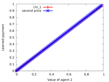
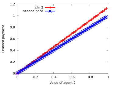
Figure 1: Learned payment rule vs. second-price payment rule for single-item auction with $2$ agents, for $\chi_{1}$ (left) and $\chi_{2}$ (right).

6.3 Multi-Minded CAs

6.3.1 Type Distribution

Recall that in a multi-minded setting, there are $r$ items, and each agent is interested in exactly $b$ bundles. For each bundle, we use the following procedure (inspired by Sandholm’s decay distribution for the single-minded setting [23]) to determine which items are included in the bundle. We first assign an item to the bundle uniformly at random. Then with probability $\alpha$, we add another random item (chosen uniformly from the remaining items), and with probability $(1-\alpha)$ we stop. We continue this procedure until we stop or have exhausted the items. We use $\alpha=0.75$ to be consistent with [23], as they report that the winner determination problem (finding the feasible allocation that maximizes total value) is difficult for this setting of $\alpha$.

Once the bundle identities have been determined, we sample values for these bundles. Let $\mathbf{c}$ be an $r$-dimensional vector with entries chosen uniformly from $(0,1]$. For each agent $i$, let $\mathbf{d}_{i}$ be an $r$-dimensional vector with entries chosen uniformly from $(0,1]$. Each entry of $\mathbf{c}$ denotes the common value of a specific item, while each entry of $\mathbf{d}_{i}$ denotes the private value of a specific item for agent $i$. The value of bundle $S_{ij}$ is then given by

$$v_{ij}=\min_{S_{ij^{\prime}}\leq S_{ij}}\left(\frac{\langle S_{ij^{\prime}},\beta\mathbf{c}+(1-\beta)\mathbf{d}_{i}\rangle}{r}\right)^{\zeta}$$

for parameters $\beta\in[0,1]$ and $\zeta$. The inner product in the numerator corresponds to a sum over values of items, where common and private values for each item are respectively weighted with $\beta$ and $(1-\beta)$. The denominator normalizes all valuations to the interval $(0,1]$. Parameter $\zeta$ controls the degree of complementarity among items: $\zeta>1$ implies that goods are complements, whereas $\zeta<1$ means that goods are substitutes. Choosing the minimum over bundles $S_{ij^{\prime}}$ contained in $S_{ij}$ finally ensures that the resulting valuations are monotonic.

6.3.2 Outcome Rules

We use two outcome rules in our experiments. For the optimal outcome rule, the payment rule $p_{vcg}$ makes the mechanism $(g_{opt},p_{vcg})$ strategyproof. Under this payment rule, agent $i$ pays the externality it imposes on other agents. That is,

$$p_{vcg,1}(\theta)=\left(\max_{o\in\Omega}\sum_{i\neq 1}v_{i}(\theta_{i},o_{i})\right)-\sum_{i\neq 1}v_{i}(\theta_{i},g_{i}(\theta)).$$

The second outcome rule with which we experiment is a generalization of the greedy outcome rule for single-minded CA Lehmann et al. [16]. Our generalization of the greedy rule is as follows. Let $\theta$ be the agent valuations and $o_{i}(j)$ denote the $j$-th bundle desired by agent $i$. For each bundle $o_{i}(j)$, assign a score $v_{i}(\theta_{i},o_{i}(j))/\sqrt{|o_{i}(j)|}$, where $|o_{i}(j)|$ indicates the total items in bundle $o_{i}(j)$. The greedy outcome rule orders the desired bundles by this score, and takes the bundle $o_{i}(j)$ with the next highest score as long as agent $i$ has not already been allocated a bundle and $o_{i}(j)$ does not contain any items already allocated. While this greedy outcome rule has an associated payment rule that makes it strategyproof in the single-minded case, it is not implementable in the multi-minded case as the example in Appendix B shows.

6.3.3 Description of Experiments

We experiment with training sets of sizes $100$, $300$, and $500$, and validation and test sets of size $1000$. All experiments we report on are for a setting with $5$ agents, $5$ items, and $3$ bundles per agent, and use $\beta=0.5$, the RBF kernel, and parameters $C\in\{10^{4},10^{5}\}$ and $\gamma\in\{0.01,0.1,1\}$.

6.3.4 Basic Results

		Optimal outcome rule									Greedy outcome rule
		accuracy			regret			ir-violation			accuracy			regret			ir-violation
$n$	$\zeta$	$p_{vcg}$	$\chi_{1}$	$\chi_{2}$	$p_{vcg}$	$\chi_{1}$	$\chi_{2}$	$p_{vcg}$	$\chi_{1}$	$\chi_{2}$	$p_{vcg}$	$\chi_{1}$	$\chi_{2}$	$p_{vcg}$	$\chi_{1}$	$\chi_{2}$	$p_{vcg}$	$\chi_{1}$	$\chi_{2}$
2	0.5	100	70.7	91.9	0	0.014	0.002	0.0	0.06	0.03	50.9	59.1	40.6	0.079	0.030	0.172	0.22	0.12	0.33
3	0.5	100	54.5	75.4	0	0.037	0.017	0.0	0.19	0.10	55.4	57.9	54.7	0.070	0.030	0.088	0.18	0.21	0.36
4	0.5	100	53.8	67.7	0	0.042	0.031	0.0	0.22	0.18	61.1	58.2	57.9	0.056	0.033	0.056	0.14	0.20	0.31
5	0.5	100	15.8	67.0	0	0.133	0.032	0.0	0.26	0.19	64.9	61.3	63.0	0.048	0.027	0.042	0.13	0.19	0.24
6	0.5	100	61.1	68.2	0	0.037	0.032	0.0	0.22	0.20	66.6	63.8	63.8	0.041	0.034	0.045	0.12	0.20	0.24
2	1.0	100	84.5	93.4	0	0.008	0.001	0.0	0.08	0.02	87.8	86.6	84.0	0.007	0.005	0.008	0.04	0.06	0.09
3	1.0	100	77.1	83.5	0	0.012	0.005	0.0	0.13	0.09	85.3	86.7	85.7	0.006	0.006	0.006	0.04	0.07	0.05
4	1.0	100	74.6	81.1	0	0.014	0.009	0.0	0.16	0.12	82.4	86.5	84.2	0.006	0.006	0.007	0.05	0.08	0.08
5	1.0	100	73.4	77.4	0	0.018	0.011	0.0	0.19	0.12	82.7	85.8	84.9	0.007	0.009	0.009	0.04	0.10	0.10
6	1.0	100	75.0	77.7	0	0.020	0.013	0.0	0.20	0.16	80.0	87.4	88.1	0.006	0.007	0.005	0.04	0.08	0.07
2	1.5	100	91.5	96.9	0	0.004	0.000	0.0	0.06	0.02	94.7	91.1	91.7	0.002	0.002	0.002	0.02	0.04	0.04
3	1.5	100	91.0	93.4	0	0.004	0.001	0.0	0.05	0.03	97.1	92.8	93.2	0.001	0.002	0.001	0.01	0.02	0.04
4	1.5	100	92.5	94.2	0	0.003	0.001	0.0	0.03	0.04	96.4	91.5	92.1	0.001	0.003	0.002	0.02	0.07	0.07
5	1.5	100	91.7	93.9	0	0.004	0.002	0.0	0.06	0.03	97.5	90.5	91.4	0.001	0.004	0.002	0.01	0.06	0.04
6	1.5	100	91.9	93.7	0	0.003	0.001	0.0	0.05	0.04	98.4	92.2	92.8	0.000	0.003	0.002	0.01	0.06	0.06

Table 2: Results for multi-minded CA with training set size 500.

Table 6.3.4 presents the basic results for multi-minded CAs with optimal and greedy outcome rules, respectively. For both outcome rules, we present the results for $p_{vcg}$ as a baseline. Because $p_{vcg}$ is the strategyproof payment rule for the optimal outcome rule, $p_{vcg}$ always has accuracy $100$, regret $0$, and IR violation $0$ for the optimal outcome rule.

Across all instances, as expected, accuracy is negatively correlated with regret and ex post IR violation. The degree of complementarity between items, $\zeta$, as well as the outcome rule chosen, has a major effect on the results. Instances with low complementarity ($\zeta=0.5$) yield payment rules with higher regret, and $\chi_{1}$ performs better on the greedy outcome rule while $\chi_{2}$ performs better on the optimal outcome rule. For high complementarity between items the greedy outcome tends to allocate all items to a single agent, and the learned price function sets high prices for small bundles to capture this property. For low complementarity the allocation tends to be split and less predictable. Still, the best classifiers achieve average ex post regret of less than 0.032 (for values normalized to [0,1]) even though the corresponding prediction accuracy can be as low as 67%. For the greedy outcome rule, the performance of $p_{vcg}$ is comparable for $\zeta\in\{1.0,1.5\}$ but worse than the payment rule learned in our framework in the case of $\zeta=0.5$, where the greedy outcome rule becomes less optimal.

Table 3: Effect of training set size on accuracy of learned classifier. Multi-minded CA, greedy outcome rule. Training set size is given in the column labels for $\chi_{1},\chi_{2}$. $p_{vcg}$ does not have a training set size.

6.3.5 Effect of Training Set Size

Table 6.3.4 charts performance as the training set size is varied for the greedy outcome rule. While training data is readily available (we can simply sample from $D$ and run the outcome rule $g$), training time becomes prohibitive for larger training set sizes. Table 6.3.4 shows that regret decreases with larger training sets, and for a training set size of 500, the best of $\chi_{1}$ and $\chi_{2}$ outperforms $p_{vcg}$ for $\zeta=0.5$ and is comparable to $p_{vcg}$ for $\zeta\in\{1.0,1.5\}$.

6.3.6 IR Fixes

Table 4: Impact of payment offset and null loss fix for $\zeta=0.5$ and greedy outcome rule, training set size 300. All results are for $\chi_{2}$, null loss values appear in the second row.

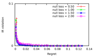
Figure 2: Impact of payment offset and null loss fix for greedy outcome rule, training set size 300.

Table 6.3.4 summarizes our results regarding the various fixes to IR violations, for the particularly challenging case of the greedy outcome rule and $\zeta=0.5$. The extent of IR violation decreases with larger payment offset and null loss. Regret tends to move in the opposite direction, but there are cases where IR violation and regret both decrease. The three rightmost columns of Table 6.3.4 list the average ratio between welfare after and before the deallocation fix, across the instances in the test set. With a payment offset of $0$, a large welfare hit is incurred if we deallocate agents with IR violations. However, this penalty decreases with increasing payment offsets and increasing null loss. At the most extreme payment offset and null loss adjustment, the IR violation is as low as $2\%$, and the deallocation fix incurs a welfare loss of only $7\%$.

Figure 2 shows a graphical representation of the impact of payment offsets and null losses. Each line in the plot corresponds to a payment rule learned with a different null loss, and each point on a line corresponds to a different payment offset. The payment offset is zero for the top-most point on each line, and equal to $0.29$ for the lowest point on each line. Increasing the payment offset always decreases the rate of IR violation, but may decrease or increase regret. Increasing null loss lowers the top-most point on a given line, but arbitrarily increasing null loss can be harmful. Indeed, in the figure on the left, a null loss of $1.5$ results in a slightly higher top-most point but significantly lower regret at this top-most point compared to a null loss of $2.0$. It is also interesting to note that these adjustments have much more impact on the hardest distribution with $\zeta=0.5$.

$n$	$\zeta$	accuracy		regret		ir-violation
		$\chi_{2}$	$\chi_{2}$ (i-mon)	$\chi_{2}$	$\chi_{2}$ (i-mon)	$\chi_{2}$	$\chi_{2}$ (i-mon)
2	0.5	46.9	46.3	0.098	0.232	0.28	0.38
3	0.5	54.4	8.6	0.082	0.465	0.33	0.06
4	0.5	58.5	48.2	0.061	0.811	0.31	0.25
5	0.5	61.8	57.0	0.048	0.136	0.26	0.26
6	0.5	63.9	61.3	0.049	0.078	0.25	0.20
2	1.0	84.1	82.2	0.008	0.010	0.06	0.08
3	1.0	80.6	80.1	0.009	0.010	0.10	0.09
4	1.0	83.1	79.7	0.009	0.012	0.11	0.11
5	1.0	84.3	77.2	0.009	0.020	0.10	0.11
6	1.0	88.3	83.9	0.005	0.013	0.08	0.11
2	1.5	89.8	89.1	0.002	0.003	0.03	0.06
3	1.5	91.5	91.3	0.002	0.003	0.04	0.04
4	1.5	90.8	89.7	0.003	0.003	0.06	0.06
5	1.5	90.5	87.3	0.003	0.005	0.04	0.05
6	1.5	92.5	70.8	0.002	0.081	0.06	0.17

Table 5: Comparison of performance with and without optimistically assuming item monotonicity. (i-mon) indicates a payment rule learned by optimistically assuming item monotonicity. Greedy outcome rule. Training set size 300.

6.3.7 Item Monotonicity

Table 5 presents a comparison of a payment rule learned with explicit enumeration of all bundle constraints (the default that we have been using for our other results) and a payment rule learned by optimistically assuming item monotonicity (see Section 5.1.3). Performance is affected when we drop constraints and optimistically assume item monotonicity, although the effects are small for $\zeta\in\{1.0,1.5\}$ and larger for $\zeta 5=0.5$. Because item monotonicity allows for the training problem to be succinctly specified, we may be able to train on more data, and this seems a very promising avenue for further consideration (perhaps coupled with heuristic methods to add additional constraints to the training problem).

6.4 The Assignment Problem

In the assignment problem, agents’ values for the items are sampled uniformly and independently from $[0,1]$. We use a training set of size $600$, validation and test sets of size $1000$, and the RBF kernel with parameters $C\in\{10,1000,100000\}$ and $\gamma\in\{0.1,0.5,1.0\}$.

The performance of the learned payment rules is compared to that of three VCG-based payment rules. Let $W$ be the total welfare of all agents other than $i$ under the outcome chosen by $g$, and $W_{eg}$ be the minimum value any agent other than $i$ receives under this outcome. We then consider the following payment rules: (1) the vcg payment rule, where agent $i$ pays the difference between the maximum total welfare of the other agents under any allocation and $W$; (2) the tot-vcg payment rule, where agent $i$ pays the difference between the total welfare of the other agents under the allocation maximizing egalitarian welfare and $W$; and (3) the eg-vcg payment rule, where agent $i$ pays the difference between the minimum value of any agent under the allocation maximizing egalitarian welfare and $W_{eg}$.

Table 6: Results for assignment problem with egalitarian outcome rule

The results for attribute map $\chi_{3}$ are shown in Table 6.3.4. We see that the learned payment rule $p_{w}$ yields significantly lower regret than any of the VCG-based payment rules, and average ex post regret less than $0.074$ for values normalized to $[0,1]$. Since we are not maximizing the sum of values of the agents, it is not very surprising that VCG-based payment rules perform rather poorly. The learned payment rule $p_{w}$ can adjust to the outcome rule, and also achieves a low fraction of ex post IR violation of at most $3\%$.

7 Conclusions

We have introduced a new paradigm for computational mechanism design in which statistical machine learning is adopted to design payment rules for given algorithmically specified outcome rules, and have shown encouraging experimental results. Future directions of interest include (1) an alternative formulation of the problem as a regression rather than classification problem, (2) constraints on properties of the learned payment rule, concerning for example the core or budgets, (3) methods that learn classifiers more likely to induce feasible outcome rules, so that these learned outcome rules can be used, (4) optimistically assuming item monotonicity and dropping constraints implied by it, thereby allowing for better scaling of training time with training set size at the expense of optimizing against a subset of the full constraints in the training problem, and (5) an investigation of the extent to which alternative goals such as regret percentiles or interim regret can be achieved through machine learning.

Acknowledgments

We thank Shivani Agarwal, Vince Conitzer, Amy Greenwald, Jason Hartline, and Tim Roughgarden for valuable discussions and the anonymous referees for helpful feedback. All errors remain our own. This material is based upon work supported in part by the National Science Foundation under grant CCF-1101570, the Deutsche Forschungsgemeinschaft under grant FI 1664/1-1, an EURYI award, and an NDSEG fellowship.

Appendix A Efficient Computation of Inner Products

For both $\chi_{1}$ and $\chi_{2}$, computing inner products reduces to the question of whether inner products between valuation profiles are efficiently computable. For $\chi_{1}$, we have that

$$\left\langle\chi_{1}(\theta_{-1},o_{1}),\chi_{1}(\theta_{-1}^{\prime},o_{1}^{\prime})\right\rangle =\mathbf{I}_{o_{1}=o_{1}^{\prime}}\sum_{i=2}^{n}\left\langle\theta_{i},\theta^{\prime}_{i}\right\rangle,$$

where indicator $$\mathbf{I}_{o_{1}=o_{1}^{\prime}}=1 o_{1}=o_{1}^{\prime} \mathbf{I}_{o_{1}=o_{1}^{\prime}}=0 \chi_{2}$$ if and otherwise. For ,

$$\left\langle\chi_{2}(\theta_{-1},o_{1}),\chi_{2}(\theta_{-1}^{\prime},o_{1}^{\prime})\right\rangle =\sum_{i=2}^{n}\left\langle\theta_{i}\setminus o_{1},\theta^{\prime}_{i}\setminus o_{1}\right\rangle.$$

We next develop efficient methods for computing the inner products $\left\langle\theta_{i},\theta^{\prime}_{i}\right\rangle$ on compactly represented valuation functions. The computation of $\left\langle\theta_{i}\setminus o_{1},\theta^{\prime}_{i}\setminus o_{1}\right\rangle$ can be done through similar methods.

In the single-minded setting, let $\theta_{i}$ correspond to a bundle $S_{i}\subseteq\{1,\ldots,r\}$ of items with value $v_{i}$, and $\theta^{\prime}_{i}$ correspond to a set $S^{\prime}_{i}\subseteq\{1,\ldots,r\}$ of items valued at $v^{\prime}_{i}$.

Each set containing both $S_{i}$ and $S^{\prime}_{i}$ contributes $v_{i}v^{\prime}_{i}$ to $\theta_{i}^{T}\theta^{\prime}_{i}$, while all other sets contribute $0$. Since there are exactly $2^{r-|S_{i}\cup S^{\prime}_{i}|}$ sets containing both $S_{i}$ and $S^{\prime}_{i}$, we have

$$\theta_{i}^{T}\theta^{\prime}_{i}=v_{i}v^{\prime}_{i}2^{r-|S_{i}\cup S^{\prime}_{i}|}.$$

This is a special case of the formula for the multi-minded case.

Lemma 2.

Consider a multi-minded CA and two bid vectors $x_{1}$ and $x^{\prime}_{1}$ corresponding to sets $S=\{S_{1},\dots,S_{s}\}$ and $S^{\prime}=\{S^{\prime}_{1},\dots,S^{\prime}_{t}\}$, with associated values $v_{1},\dots,v_{s}$ and $v^{\prime}_{1},\dots,v^{\prime}_{t}$. Then,

$$x_{1}^{T}x^{\prime}_{1}=\sum_{T\subseteq S,T^{\prime}\subseteq S^{\prime}}\Bigl{(}(-1)^{|T|+|T^{\prime}|}\cdot(\min_{S_{i}\in T}v_{i})\cdot(\min_{S^{\prime}_{j}\in T^{\prime}}v^{\prime}_{j})\cdot 2^{r-|(\bigcup_{S_{i}\in T}S_{i})\cup(\bigcup_{S^{\prime}_{j}\in T^{\prime}}S^{\prime}_{j})|}\Bigr{)}.$$ (4)

Proof.

The contribution of a particular bundle $B$ of items to the inner product is $(\max_{S_{i}\in S,S_{i}\subseteq B}v_{i})\cdot(\max_{S^{\prime}_{j}\in S^{\prime},S^{\prime}_{j}\subseteq B}v^{\prime}_{j})$, and thus

$$x_{1}^{T}x^{\prime}_{1}=\sum_{B}\Bigl{(}(\max_{\genfrac{}{}{0.0pt}{}{S_{i}\in S}{S_{i}\subseteq B}}v_{i})\cdot(\max_{\genfrac{}{}{0.0pt}{}{S^{\prime}_{j}\in S^{\prime}}{S^{\prime}_{j}\subseteq B}}v^{\prime}_{j})\Bigr{)}.$$

By the maximum-minimums identity, which asserts that for any set $\{x_{1},\dots,x_{n}\}$ of $n$ numbers, $\max\{x_{1},\dots,x_{n}\}=\sum_{Z\subseteq X}((-1)^{|Z|+1}\cdot(\min_{x_{i}\in Z}x_{i}))$,

$$\max_{\genfrac{}{}{0.0pt}{}{S_{i}\in S}{S_{i}\subseteq B}}v_{i}=\sum_{\genfrac{}{}{0.0pt}{}{T\subseteq S}{\mathchoice{\hbox to0.0pt{\hss$\displaystyle{\bigcup_{S_{i}\in T}S_{i}\subseteq B}$\hss}}{\hbox to0.0pt{\hss$\textstyle{\bigcup_{S_{i}\in T}S_{i}\subseteq B}$\hss}}{\hbox to0.0pt{\hss$\scriptstyle{\bigcup_{S_{i}\in T}S_{i}\subseteq B}$\hss}}{\hbox to0.0pt{\hss$\scriptscriptstyle{\bigcup_{S_{i}\in T}S_{i}\subseteq B}$\hss}}}}\Bigl{(}(-1)^{|T|+1}\cdot(\min_{S_{i}\in T}v_{i})\Bigr{)}\quad\text{and}$$

$$\max_{\genfrac{}{}{0.0pt}{}{S^{\prime}_{j}\in S^{\prime}}{S^{\prime}_{j}\subseteq B}}v^{\prime}_{j}=\sum_{\genfrac{}{}{0.0pt}{}{T^{\prime}\subseteq S^{\prime}}{\mathchoice{\hbox to0.0pt{\hss$\displaystyle{\bigcup_{S^{\prime}_{j}\in T^{\prime}}S^{\prime}_{j}\subseteq B}$\hss}}{\hbox to0.0pt{\hss$\textstyle{\bigcup_{S^{\prime}_{j}\in T^{\prime}}S^{\prime}_{j}\subseteq B}$\hss}}{\hbox to0.0pt{\hss$\scriptstyle{\bigcup_{S^{\prime}_{j}\in T^{\prime}}S^{\prime}_{j}\subseteq B}$\hss}}{\hbox to0.0pt{\hss$\scriptscriptstyle{\bigcup_{S^{\prime}_{j}\in T^{\prime}}S^{\prime}_{j}\subseteq B}$\hss}}}}\Bigl{(}(-1)^{|T^{\prime}|+1}\cdot(\min_{S^{\prime}_{j}\in T^{\prime}}v^{\prime}_{j})\Bigr{)}.$$

The inner product can thus be written as

$$\theta_{1}^{T}\theta^{\prime}_{1}=\sum_{B}\sum_{\genfrac{}{}{0.0pt}{}{T\subseteq S,T^{\prime}\subseteq S^{\prime}}{\genfrac{}{}{0.0pt}{}{\bigcup_{S_{i}\in T}S_{i}\subseteq B}{\bigcup_{S^{\prime}_{j}\in T^{\prime}}S^{\prime}_{j}\subseteq B}}}\Bigl{(}(-1)^{|T|+|T^{\prime}|}\cdot(\min_{S_{i}\in T}v_{i})\cdot(\min_{S^{\prime}_{j}\in T^{\prime}}v^{\prime}_{j})\Bigr{)}.$$

Finally, for given $T\subseteq S$ and $T^{\prime}\subseteq S^{\prime}$, there exist exactly $2^{r-|(\bigcup_{S_{i}\in T}S_{i})\cup(\bigcup_{S^{\prime}_{j}\in T^{\prime}}S^{\prime}_{j})|}$ bundles $B$ such that $\bigcup_{S_{i}\in T}S_{i}\subseteq B$ and $\bigcup_{S^{\prime}_{j}\in T^{\prime}}S^{\prime}_{j}\subseteq B$, and we obtain

$$\theta_{1}^{T}\theta^{\prime}_{1}=\sum_{T\subseteq S,T^{\prime}\subseteq S^{\prime}}\Bigl{(}(-1)^{|T|+|T^{\prime}|}\cdot(\min_{S_{i}\in T}v_{i})\cdot(\min_{S^{\prime}_{j}\in T^{\prime}}v^{\prime}_{j})\cdot 2^{m-|(\bigcup_{S_{i}\in T}S_{i})\cup(\bigcup_{S^{\prime}_{j}\in T^{\prime}}S^{\prime}_{j})|}\Bigr{)}.$$

∎

If $S$ and $S^{\prime}$ have constant size, then the sum on the right hand side of (4) ranges over a constant number of sets and can be computed efficiently.

Appendix B Greedy Allocation Rule is not Weakly Monotone

Consider a setting with a single agent and four items.

If the valuations $\theta_{1}$ of the agent are

$$v_{1}(\theta_{1},o_{1})=\begin{cases}20&\text{if $o_{1}=\{1,2,3,4\}$}\\ 12&\text{if $1\in o_{1}$ and $j\notin o_{1}$ for some $j\in\{2,3,4\}$, and}\\ 0&\text{else}\end{cases}$$

then the allocation is $\{1\}$.

If the valuations are $\theta_{1}^{\prime}$ such that

$$v_{1}(\theta_{1}^{\prime},o_{1})=\begin{cases}12&\text{if $o_{1}=\{1,2,3,4\}$}\\ 5&\text{if $1\in o_{1}$ and $j\notin o_{1}$ for some $j\in\{2,3,4\}$, and}\\ 0&\text{else}\end{cases}$$

then the allocation is $\{1,2,3,4\}$.

We have $v_{1}(\theta_{1}^{\prime},\{1,2,3,4\})-v_{1}(\theta_{1}^{\prime},\{1\})<v_{1}(\theta_{1},\{1,2,3,4\})-v_{1}(\theta_{1},\{1\})$ contradicting weak monotonicity.

References

- Ashlagi et al. [2010] I. Ashlagi, M. Braverman, A. Hassidim, and D. Monderer. Monotonicity and implementability. Econometrica, 78(5):1749–1772, 2010.
- Ausubel and Milgrom [2006] L. M. Ausubel and P. Milgrom. The lovely but lonely Vickrey auction. In P. Cramton, Y. Shoham, and P. Steinberg, editors, Combinatorial Auctions, chapter 1, pages 17–40. MIT Press, 2006.
- Budish [2010] E. Budish. The combinatorial assignment problem: Approximate competitive equilibrium from equal incomes. Working Paper, 2010.
- Cai et al. [2012] Y. Cai, C. Daskalakis, and S. M. Weinberg. An algorithmic characterization of multi-dimensional mechanisms. In Proc. of 44th STOC, page Forthcoming, 2012.
- Carroll [2011] G. Carroll. A quantitative approach to incentives: Application to voting rules. Technical report, MIT, 2011.
- Conitzer and Sandholm [2002] V. Conitzer and T. Sandholm. Complexity of mechanism design. In Proc. of 18th UAI Conference, pages 103–110, 2002.
- Day and Milgrom [2008] R. Day and P. Milgrom. Core-selecting package auctions. International Journal of Game Theory, 36(3–4):393–407, 2008.
- Erdil and Klemperer [2010] A. Erdil and P. Klemperer. A new payment rule for core-selecting package auctions. Journal of the European Economic Association, 8(2–3):537–547, 2010.
- Guo and Conitzer [2010] M. Guo and V. Conitzer. Computationally feasible automated mechanism design: General approach and case studies. In Proc. of 24th AAAI Conference, 2010.
- Hartline and Lucier [2010] J. D. Hartline and B. Lucier. Bayesian algorithmic mechanism design. In Proc. of 42nd STOC, pages 301–310, 2010.
- Hartline et al. [2011] J. D. Hartline, R. Kleinberg, and A. Malekian. Bayesian incentive compatibility via matchings. In Proc. of 22nd SODA, pages 734–747, 2011.
- Joachims et al. [2009] T. Joachims, T. Finley, and C.-N. J. Yu. Cutting-plane training of structural SVMs. Machine Learning, 77(1):27–59, 2009.
- Lahaie [2009] S. Lahaie. A kernel method for market clearing. In Proc. of 21st IJCAI, pages 208–213, 2009.
- Lahaie [2010] S. Lahaie. Stability and incentive compatibility in a kernel-based combinatorial auction. In Proc. of 24th AAAI Conference, pages 811–816, 2010.
- Lavi and Swamy [2005] R. Lavi and C. Swamy. Truthful and near-optimal mechanism design via linear programming. In Proc. of 46th FOCS Symposium, pages 595–604, 2005.
- Lehmann et al. [2002] D. Lehmann, L. I. O’Callaghan, and Y. Shoham. Truth revelation in approximately efficient combinatorial auctions. Journal of the ACM, 49:577–602, 2002.
- Lubin [2010] B. Lubin. Combinatorial Markets in Theory and Practice: Mitigating Incentives and Facilitating Elicitation. PhD thesis, Department of Computer Science, Harvard University, 2010.
- Lubin and Parkes [2009] B. Lubin and D. C. Parkes. Quantifying the strategyproofness of mechanisms via metrics on payoff distributions. In Proc. of 25th UAI Conference, pages 349–358, 2009.
- Parkes et al. [2001] D. C. Parkes, J. Kalagnanam, and M. Eso. Achieving budget-balance with Vickrey-based payment schemes in exchanges. In Proc. of 17th IJCAI, pages 1161–1168, 2001.
- Pathak and Sönmez [2010] P. Pathak and T. Sönmez. Comparing mechanisms by their vulnerability to manipulation. Working Paper, 2010.
- Rastegari et al. [2011] B. Rastegari, A. Condon, and K. Leyton-Brown. Revenue monotonicity in deterministic, dominant-strategy combinatorial auctions. Artificial Intelligence, 175:441–456, 2011.
- Saks and Yu [2005] M. Saks and L. Yu. Weak monotonicity suffices for truthfulness on convex domains. In Proc. of 6th ACM-EC Conference, pages 286–293, 2005.
- Sandholm [2002] T. Sandholm. Algorithm for optimal winner determination in combinatorial auctions. Artificial Intelligence, 135(1-2):1–54, 2002.
- Tsochantaridis et al. [2005] I. Tsochantaridis, T. Joachims, T. Hofmann, and Y. Altun. Large margin methods for structured and interdependent output variables. Journal of Machine Learning Research, 6:1453–1484, 2005.