The Quark and Gluon Structure of the Proton

E. Perez^a and E. Rizvi^b

^a CERN, PH Department, Geneva, CH

^b Queen Mary University of London, School of Physics and Astronomy,
London, UK

In this article we present a review of the structure of the proton and the current status of our knowledge of the parton distribution functions (PDFs). The lepton-nucleon scattering experiments which provide the main constraints in PDF extractions are introduced and their measurements are discussed. Particular emphasis is given to the HERA data which cover a wide kinematic region. Hadron-hadron scattering measurements which provide supplementary information are also discussed. The methods used by various groups to extract the PDFs in QCD analyses of hard scattering data are presented and their results are compared. The use of existing measurements allows predictions for cross sections at the LHC to be made. A comparison of these predictions for selected processes is given. First measurements from the LHC experiments are compared to predictions and some initial studies of the impact of this new data on the PDFs are presented.

Submitted to Reports on Progress in Physics.

1 Introduction

The birth of modern experimental particle physics in which particles were used to probe the structure of composite objects began with the famous alpha particle scattering experiment of Geiger and Marsden under the direction of Rutherford. In 1911 Rutherford published an analysis of the data providing evidence for atomic structure consisting of a massive positively charged nucleus surrounded by electrons [1]. Since then the use of particle probes to deduce structure has become standard, albeit at increasingly higher energy and intensity which brings its own technological and experimental challenges.

Experiments of point-like electrons scattering off extended objects such as nuclei were expected to deviate from the predictions of Mott scattering - relativistic electron-electron Coulomb scattering [2]. This deviation, the nuclear form factor (expressed in terms of the 4-momentum transfer $Q$ between initial and final state electrons), was shown to be related to the Fourier transform of the nuclear charge density [3, 4]. In 1955 Hofstadter measured nuclear form factors with a $100-500$ MeV electron beam and obtained the charge density of the proton and other atomic nuclei [5, 6, 7]. The experiment was able to resolve the proton’s charge radius to $\simeq~{}0.7$ fm, at least an order of magnitude better than Rutherford’s experiment.

The idea that nucleons were composite particles was first proposed in 1964 by Zweig [8] and Gell-Mann [9]. Their quark model represented an underlying schema to classify the static properties of the known hadrons. However, this model had difficulties explaining why direct production of quarks did not occur.

Detailed study of the structure of the proton advanced in 1967 when a $20$ GeV linear electron accelerator commenced operation at the Stanford Linear Accelerator Centre (SLAC) with the aim of studying inelastic proton scattering, resonance production and the inelastic continuum in the region of $0.7\leq Q^{2}\leq 25$ GeV². This opened the field of deep inelastic scattering (DIS) in which the nucleon target was dissociated to large invariant mass states in the interaction. First observations of elastic scattering showed a rapid $1/Q^{4}$ behaviour of the cross section [10] as expected from earlier low energy elastic form factor measurements at SLAC, Cornell, DESY and CEA [11, 12, 13, 14, 15, 16]. This was found to be in stark contrast to the weaker $Q^{2}$ dependence of the inelastic cross section in the same energy range [17, 18].

For inelastic Coulomb scattering two form factors are required to describe the cross section, the so-called structure functions, which at fixed lepton beam energy can only depend on two kinematic quantities taken to be $Q^{2}$ and the electron energy loss in the nucleon rest frame, $\nu$ [19]. The SLAC structure function measurements were found to exhibit scaling behaviour i.e. were independent of $Q^{2}$. This behaviour had been predicted by Bjorken [20] in the same year.

The new SLAC data prompted Feynman to develop the parton model of deep inelastic scattering [21] in which the scaling behaviour is naturally explained as the point-like elastic scattering of free partons within the protons. Bjorken and Paschos then further developed the quark-parton model [22]. In the same year Callan and Gross showed that the behaviour of the longitudinally polarised part of the virtual photon scattering cross section required the constituents to be spin $\frac{1}{2}$ fermions [23]. The association of these point-like constituents as the quarks of Gell-Mann and Zweig was gradually made and widely accepted by 1974.

The inability to observe free quarks (confinement) and the free quarks of the parton model was a contradiction that was solved through the idea of a scale dependant coupling which was large at low energy and feeble at high energies [24, 25]. This lead to the rapid development of quantum-chromodynamics (QCD) which was soon established as the correct theory of strong interactions.

A wider programme of scattering experiments followed providing detailed insight into the structure of the proton and electroweak (EW) interactions between the quark and lepton sectors of the Standard Model. First observations of weak neutral currents by the Gargamelle neutrino-nucleon experiment [26, 27] were made in 1973, scaling violations of DIS cross sections were observed in 1974 [28], and the discovery of the gluon was made in 1979 by the TASSO $e^{+}e^{-}$ experiment [29] at DESY.

In 1993-2007 HERA, the only $ep$ collider, operated at DESY and opened up a wide kinematic region for precision measurements of proton structure and was capable of resolving structures to $10^{-3}$ fm. The precise HERA data together with fixed target DIS measurements and data from hadro-production experiments strongly constrain the proton’s parton distributions.

Experiments at CERN, DESY, SLAC and JLab (see for example [30, 31, 32, 33, 34, 35]) have extensively studied polarised DIS to understand how the proton’s spin arises from the orbital and intrinsic angular momenta of the constituent partons. In this article we omit any discussion of spin although a review of the field can be found for example in [36, 37].

The knowledge that we now have of QCD and proton structure is a vital tool in helping disentangle and interpret potential signals of new physics at the Large Hadron Collider (LHC) at CERN which has commenced operation colliding protons at a centre-of-mass energy $\sqrt{s}$ of up to $8$ TeV, and is expected to reach the design value of about $14$ TeV in the next few years.

In this report we review the current status of our understanding of proton structure. In section 1.1 and the remaining sections of this chapter the formalism for deep inelastic scattering is given and the parton distribution functions (PDFs) are introduced. A more formal introduction can be found for example in [38]. The experimental constraints on the proton structure measurements are discussed in detail in chapter 2 including data from non-DIS experiments. Chapter 3 provides an overview of the methods used to extract the PDFs from the various experimental measurements. Finally in chapter 4 the potential of the LHC in constraining our knowledge of proton structure is discussed.

1.1 Kinematic Quantities in DIS

In this section we outline the general formalism for unpolarised deeply inelastic lepton-nucleon scattering in perturbative QCD. Inclusive neutral current (NC) scattering of a charged lepton $l$ off a nucleon $N$ proceeds via the reaction $l^{\pm}N\rightarrow l^{\pm}X$ and the exchange of virtual neutral electroweak vector bosons, $\gamma$ or $Z^{0}$. Here $X$ represents any final state. The purely weak charged current (CC) process is $l^{\pm}N\rightarrow\overset{\raisebox{-3.0pt}{\scalebox{0.4}{ {(}}}\raisebox{-2.0pt}{{\_}}\raisebox{-3.0pt}{\scalebox{0.4}{{)}}}}{\nu}X$ and occurs via exchange of a virtual $W^{\pm}$ boson.

The measured cross sections are usually expressed in terms of three variables $x$, $y$ and $Q^{2}$ defined as

$$x=\frac{Q^{2}}{2p\cdot q}\hskip 56.9055pty=\frac{p\cdot q}{p\cdot k}\hskip 56.9055ptQ^{2}=-q^{2}\equiv-(k-k^{\prime})^{2}\,\,,$$ (1)

where $k$ and $k^{\prime}$ are the momenta of the initial and scattered lepton, $p$ is the nucleon momentum, and $q$ the momentum of the exchanged boson (see Fig. 1). The first of these, also known as $x_{Bjorken}$, is the fraction of the target nucleon’s momentum taken by the parton in the infinite momentum frame where the partons have zero transverse momenta. The inelasticity is measured by the quantity $y$ and is the fractional energy loss of the lepton in the rest frame of the target nucleon. It also quantifies the lepton-parton scattering angle $\theta^{*}$ measured with respect to the lepton direction in the centre-of-mass frame since $y=\frac{1}{2}(1-\cos\theta^{*})$. The 4-momentum transfer squared from the lepton $Q^{2}$, quantifies the virtuality of the exchange boson. The three quantities are related to the lepton-nucleon centre-of-mass energy, $\sqrt{s}$, via $Q^{2}=sxy$ which holds in the massless approximation since $s=(k+p)^{2}$. Thus for fixed centre-of-mass energy the cross sections are dependant on only two quantities. Modern experiments typically publish measured cross sections differentially in two variables, usually $x$ and $Q^{2}$ or $x$ and $y$.

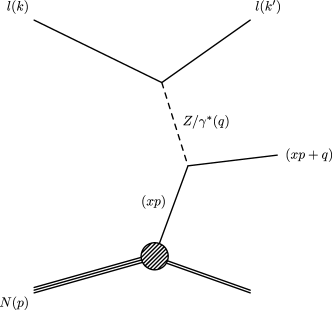
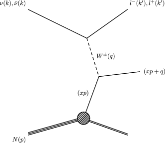
Figure 1: Left: Schematic diagram of NC DIS of a charged lepton $l$ with incoming and outgoing momenta $k$ and $k^{\prime}$ interacting with nucleon $N$ with momentum $p$ via the exchange of a virtual $Z/\gamma^{*}$ boson ($q$) between the lepton and a parton carrying fractional momentum $xp$ (see text). Right: Schematic of CC neutrino induced DIS via the exchange of a virtual $W^{\pm}$ boson.

Two other related kinematic quantities are also sometimes used and are given here for completeness. They are

$$W^{2}=(q+p)^{2}=Q^{2}\frac{1-x}{x}+m_{N}^{2}\hskip 85.35826pt\nu=\frac{p\cdot q}{m_{N}}\,\,\,.$$ (2)

$W^{2}$ is the invariant mass squared of the final hadronic system, and $\nu$ is the lepton energy loss in the rest frame of the nucleon, with $m_{N}$ the nucleon mass.

1.2 The Quark Parton Model

The Quark Parton Model (QPM)  [21, 22] describes nucleons as consisting of massless point-like spin $\frac{1}{2}$ quarks which are free within the nucleon. The gluon is completely neglected, but despite this failing it is nevertheless a useful conceptual model with which to illustrate a discussion of proton structure. Nucleon and quark masses are also neglected, an approximation that is valid provided the momentum scale of the scattering process $Q$ is large enough. The parton distribution functions $f_{i}(x)$ in the QPM are number densities of parton flavour $i$ with fraction $x$ of the parent nucleon’s energy and longitudinal momentum. Often the momentum weighted distributions $xf_{i}(x)$ are used. In standard notation the anti-quark PDFs are denoted $x{\overline{f}_{i}}(x)$, and PDFs for each quark flavour are written as $u,d,s,c,b$ for the up, down, strange, charm and bottom respectively. The PDFs obey counting sum rules which for the proton are written as

$$\int_{0}^{1}\left[u(x)-\bar{u}(x)\right]\,{\rm d}x=2\hskip 56.9055pt\int_{0}^{1}\left[d(x)-\bar{d}(x)\right]\,{\rm d}x=1\,\,\,$$ (3)

$${\rm{and}}\hskip 28.45274pt\int_{0}^{1}\left[q(x)-\bar{q}(x)\right]\,{\rm d}x=0\hskip 28.45274pt{\rm{for}}\quad q=s,c,b$$ (4)

and require the valence structure of the proton to correspond to $uud$. The valence distributions are defined as $u_{v}=u-{\bar{u}}$ and $d_{v}=d-{\bar{d}}$. The constraint of momentum conservation in the QPM is written as

$$\int_{0}^{1}\sum_{i}^{n_{f}}x\left[q_{i}(x)+\bar{q_{i}}(x)\right]\,{\rm d}x=1$$ (5)

where the sum runs over all active parton flavours $n_{f}$.

Deeply inelastic lepton-nucleon scattering cross sections are calculated from incoherent sums of elastic lepton-parton processes. More generally, the hadronic interaction cross section for a process $A+B\rightarrow X$ can be written as

$$\sigma_{A,B\rightarrow X}=\sum_{i,j}\iint f_{i}^{A}(x_{1})\cdot f_{j}^{B}(x_{2})\cdot\hat{\sigma}_{i,j\rightarrow X}\,dx_{1}dx_{2}+[x_{1}\leftrightarrow x_{2}]$$ (6)

where $\hat{\sigma}_{i,j\rightarrow X}$ is the partonic cross section for interactions of two partons with flavour $i$ and $j$. The fact that the PDFs in Eq. 6 are universal is known as the factorisation property: PDFs extracted from an analysis of e.g. inclusive DIS measurements can be used to calculate the cross sections of other processes in lepton-hadron or hadron-hadron interactions. A proof of the factorisation theorem in perturbative QCD can be found in [39].

The QPM represents the lowest order approximation of QCD and as such does not take into account gluon contributions to the scattering process. This implies a scale ($Q$) invariance to all QPM predictions known as Bjorken scaling - the quarks are free within the nucleon and thus do not exchange momenta. Early DIS measurements [17, 18] demonstrated approximate scaling behaviour for $x\approx 0.3$ indicating the scattering of point-like constituents of the proton, but subsequent measurements extended over a wider $x$ range showed that scaling behaviour is violated [28]. This is interpreted as being due to gluon radiation suppressing high $x$ partons and creating a larger density of low $x$ partons with increasing $Q^{2}$. Thus in the absence of scaling, the PDFs $f_{i}(x)$ become $Q^{2}$ dependent, $f_{i}(x,Q^{2})$.

It is usual to consider the neutron PDFs ($f_{i}^{n}$) as being related to the proton PDFs ($f_{i}^{p}$) by invoking strong isospin symmetry, i.e. that $u^{p}=d^{n}$, $d^{p}=u^{n}$, $\bar{u}^{p}=\bar{d}^{n}$, $\bar{d}^{p}=\bar{u}^{n}$ and that the PDFs of other flavours remain the same for neutron and proton. This is used in order to exploit the structure function measurements performed in DIS off a deuterium target. For the remainder of this article PDFs always refer to proton PDFs.

The QPM provides a good qualitative description of scattering data. It was convincingly tested in the prediction of the $pp\rightarrow\mu^{+}\mu^{-}+X$ process  [40]. Sum rules similar to those in Eqs. 3 and 5 such as the Gross-Llewellyn-Smith (GLS) [41], Adler [42], Bjorken [43] and Gottfried [44] sum rules were also well predicted by the QPM (for details see [45, 46]).

1.3 DIS Formalism

The scattering of a virtual boson off a nucleon can be written in terms of a leptonic and a hadronic tensor with appropriate couplings of the exchanged boson to the lepton and the partons (see for example [46]). The hadronic tensor is not calculable from first principles and is expressed in terms of three general structure functions which for NC processes are $\tilde{F}_{2}$, $x\tilde{F}_{3}$ and $\tilde{F}_{L}$. The total virtual boson absorption cross section is related to the $\tilde{F}_{2}$ and $x\tilde{F}_{3}$ parts in which both the longitudinal and the transverse polarisation states of the virtual boson contribute, whereas only the longitudinally polarised piece contributes to $\tilde{F}_{L}$. These NC structure functions can be further decomposed into pieces relating to pure photon exchange, pure $Z^{0}$ exchange and an interference piece.

At the Born level the NC cross section for the process $e^{\pm}p\rightarrow e^{\pm}X$ is given by

$$\frac{{\rm d}^{2}\sigma_{NC}^{\pm}}{{\rm d}x\;{\rm d}\mbox{${Q^{2}}$}} = \frac{2\pi\alpha^{2}}{xQ^{4}}\left[Y_{+}\mbox{$\tilde{F}_{2}$}\mp Y_{-}x\mbox{$\tilde{F}_{3}$}-y^{2}\mbox{$\tilde{F}_{{}_{L}}$}\right]$$ (7)

where $\alpha\equiv\alpha(Q^{2}=0)$ is the fine structure constant. The helicity dependencies of the electroweak interactions are contained in $Y_{\pm}\equiv 1\pm(1-y)^{2}$.

The generalised proton structure functions [47], $\tilde{F}_{L,2,3}$, may be written as linear combinations of the hadronic structure functions $F_{L,2}$, $F_{L,2,3}^{\gamma Z}$, and $F_{L,2,3}^{Z}$ containing information on QCD parton dynamics as well as the EW couplings of the quarks to the neutral vector bosons. The function $F_{2}$ is associated to pure photon exchange terms, $F_{L,2,3}^{\gamma Z}$ correspond to photon-$Z^{0}$ interference and $F_{L,2,3}^{Z}$ correspond to the pure $Z^{0}$ exchange terms. Neglecting $\tilde{F}_{L}$, the linear combinations for arbitrary longitudinal lepton polarised $e^{\pm}p$ scattering are given by

$$\tilde{F}^{\pm}_{2}=F_{2}-(v_{e}\pm Pa_{e})\kappa\frac{Q^{2}}{Q^{2}+M_{Z}^{2}}F_{2}^{\gamma Z}+(v_{e}^{2}+a_{e}^{2}\pm 2Pv_{e}a_{e})\kappa^{2}\left[\frac{Q^{2}}{Q^{2}+M_{Z}^{2}}\right]^{2}F_{2}^{Z}$$ (8)

$$x\tilde{F}^{\pm}_{3}=-(a_{e}\pm Pv_{e})\kappa\frac{Q^{2}}{Q^{2}+M_{Z}^{2}}xF_{3}^{\gamma Z}+(2a_{e}v_{e}\pm P[v_{e}^{2}+a_{e}^{2}])\kappa^{2}\left[\frac{Q^{2}}{Q^{2}+M_{Z}^{2}}\right]^{2}xF_{3}^{Z}$$ (9)

where $P$ is the degree of lepton polarisation, $a_{e}$ and $v_{e}$ are the usual leptonic electroweak axial and vector couplings to the $Z^{0}$ and $\kappa$ is defined by $\kappa^{-1}=4\frac{M_{W}^{2}}{M_{Z}^{2}}(1-\frac{M_{W}^{2}}{M_{Z}^{2}})$, $M_{W}$ and $M_{Z}$ being the masses of the electroweak bosons.

The structure function $\tilde{F}_{{}_{L}}$ (proportional to the longitudinally polarised virtual photon scattering cross section, $\sigma_{L}$) may be decomposed in a manner similar to $\tilde{F}_{2}$ (proportional to the sum of longitudinally and transversely polarised virtual photon scattering cross sections $\sigma_{L}+\sigma_{T}$). Its contribution is significant only at high $y$ (see Eq. 7). The ratio $R$ defined as $R(x,Q^{2})=\sigma_{L}(x,Q^{2})/\sigma_{T}(x,Q^{2})=F_{L}/(F_{2}-F_{L})$ is often used instead of $F_{L}$ to describe the scattering cross section. The QPM predicts that longitudinally polarised virtual photon scattering is forbidden due to helicity conservation considerations, i.e. $F_{L}=0$ for spin half partons. The fact that $F_{L}$ is non-zero is a consequence of the existence of gluons and QCD as the underlying theory.

Over most of the experimentally accessible kinematic domain the dominant contribution to the NC cross section comes from the electromagnetic structure function $F_{2}$. Only at large values of $Q^{2}$ do the contributions from $Z^{0}$ boson exchange become important. For longitudinally unpolarised lepton beams $\tilde{F}_{2}$ is the same for $e^{-}$ and for $e^{+}$ scattering, while the $x\mbox{$\tilde{F}_{3}$}$ contribution changes sign as can be seen in Eq. 7.

In the QPM the structure functions $F_{2}$, $F_{2}^{\gamma Z}$ and $F_{2}^{Z}$ are related to the sum of the quark and anti-quark densities

$$[F_{2},F_{2}^{\gamma Z},F_{2}^{Z}]=x\sum_{q}[e_{q}^{2},2e_{q}v_{q},v_{q}^{2}+a_{q}^{2}]\{q+\bar{q}\}$$ (10)

and the structure functions $xF_{3}^{\gamma Z}$ and $xF_{3}^{Z}$ to their difference which determines the valence quark distributions $q_{v}$

$$[xF_{3}^{\gamma Z},xF_{3}^{Z}]=2x\sum_{q}[e_{q}a_{q},v_{q}a_{q}]\{q-\bar{q}\}=2x\sum_{q}[e_{q}a_{q},v_{q}a_{q}]q_{v}\,\,\,.$$ (11)

Here $e_{q}$ is the charge of quark $q$ in units of the positron charge and $v_{q}$ and $a_{q}$ are the vector and axial-vector weak coupling constants of the quarks to the $Z^{0}$.

For CC interactions the Born cross section may be expressed as

$$\frac{{\rm d}^{2}\sigma_{\rm CC}^{\pm}}{{\rm d}x\;{\rm d}Q^{2}} = (1\pm P)\frac{G_{F}^{2}}{4\pi x}\left[\frac{M_{W}^{2}}{Q^{2}+M_{W}^{2}}\right]^{2}\;(Y_{+}W_{2}(lp)\mp Y_{-}xW_{3}(lp)-y^{2}W_{L}(lp))$$ (12)

where $\sigma^{+}_{CC}$ ($\sigma^{-}_{CC}$) denotes the cross section for $e^{+}p$ or $\bar{\nu}p$ ($e^{-}p$ or $\nu p$) interactions. In the case of (anti-)neutrino interactions, $1\pm P=2$ in Eq.12. The weak coupling is expressed here as the Fermi constant $G_{F}$. The CC structure functions $W_{2}$, $W_{3}$ and $W_{L}$ are defined in a similar manner to the NC structure functions [48]. In the QPM (where $W_{L}\equiv 0$) they may be interpreted as sums and differences of quark and anti-quark densities and are given by

$$W_{2}(e^{+}p)=W_{2}(\nu p)=x(\bar{U}+D)\hskip 2.84544pt\mbox{,}\hskip 8.5359pt xW_{3}(e^{+}p)=xW_{3}(\nu p)=x(D-\bar{U})\hskip 2.84544pt\mbox{,}\hskip 8.5359pt$$ (13)

$$W_{2}(e^{-}p)=W_{2}(\bar{\nu}p)=x(U+\bar{D})\hskip 2.84544pt\mbox{,}\hskip 8.5359pt xW_{3}(e^{-}p)=xW_{3}(\bar{\nu}p)=x(U-\bar{D})\,\,\,$$ (14)

where $U$ represents the sum of up-type, and $D$ the sum of down-type quark densities,

$$U = u+c$$

$$\bar{U} = \bar{u}+\bar{c}$$

$$D = d+s+b$$

$$\bar{D} = \bar{d}+\bar{s}+\bar{b}.$$ (15)

Neutrino DIS experiments generally use a heavy target to compensate for the low interaction rates. For an isoscalar target, i.e. with the same number of protons and neutrons, the structure functions become, assuming $q=\bar{q}$ for $q=s,c,b$ :

$$W_{2}(\nu N)=W_{2}(\bar{\nu}N) = x(U+D+\bar{U}+\bar{D})\qquad,$$ (16)

$$W_{3}(\nu N) = x(u_{v}+d_{v}+2s+2b-2\bar{c})\qquad,$$ (17)

$$W_{3}(\bar{\nu}N) = x(u_{v}+d_{v}-2\bar{s}-2\bar{b}+2c)\qquad,$$ (18)

such that the difference between $\nu N$ and $\bar{\nu}N$ cross sections is directly sensitive to the total valence distribution.

Some analyses of DIS cross sections present the data in terms of “reduced cross sections” where kinematic pre-factors are factored out to ease visualisation. Typically they are defined as:

$$\tilde{\sigma}_{NC}(x,Q^{2})\equiv\frac{1}{Y_{+}}\ \frac{Q^{4}\ x}{2\pi\alpha^{2}}\ \frac{{\rm d}^{2}\sigma_{NC}}{{\rm d}x{\rm d}Q^{2}},\;\;\;\tilde{\sigma}_{CC}(x,Q^{2})\equiv\frac{2\pi x}{G_{F}^{2}}\left[\frac{M_{W}^{2}+Q^{2}}{M_{W}^{2}}\right]^{2}\frac{{\rm d}^{2}\sigma_{CC}}{{\rm d}x{\rm d}Q^{2}}.\;\;\;$$ (19)

1.4 QCD and the Parton Distribution Functions

The QPM is based on an apparent contradiction that DIS scattering cross sections may be determined from free quarks which are bound within the nucleon. Despite this the QPM was very successful at being able to take PDFs from one scattering process and predicting cross sections for other scattering experiments; it nevertheless has difficulties. The first of these is the failure of the model to accurately describe violations of scaling and scale dependence of DIS cross sections. The fact that partons are strongly bound into colourless states is an experimental fact, but why they behave as free particles when probed at high momenta is not explained. The QPM is also unable to account for the full momentum of the proton via measurements of the momentum sum rule of Eq. 5 indicating the existence of a new partonic constituent which does not couple to electroweak probes, the gluon ($g$), which modifies the momentum sum rule as below:

$$\int_{0}^{1}\sum_{i}x\left[q_{i}(x)+\bar{q_{i}}(x)\right]+xg(x)\,{\rm d}x=1$$ (20)

It is only by including the effects of the gluon and gluon radiation in hard scattering processes that an accurate description of experimental data can be given. These developments led to the formulation of quantum-chromodynamics.

Any theory of QCD must be able to accommodate the twin concepts of asymptotic freedom and confinement. The former applies at large scales ($Q$) where experiments are able to resolve the partonic content of hadrons which are quasi-free in the high energy (short time-scale) limit, and is a unique feature of non-abelian theories. The latter explains the strong binding of partons into colourless observable hadrons at low energy scales (or equivalently, over long time-scales). In 1973 Gross, Wilczek and Politzer [24, 25] showed that perturbative non-abelian field theories could give rise to asymptotically free behaviour of quarks and scaling violations. By introducing a scale dependent coupling strength $\alpha_{s}(Q)=g^{2}/4\pi$ (where $g$ is the QCD gauge field coupling and depends on $Q$), confinement and asymptotic freedom can be accommodated in a single theory. Perturbative QCD (pQCD) is restricted to the region where the $\alpha_{s}$ coupling is small enough to allow cross sections to be calculated as a rapidly convergent power series in $\alpha_{s}$. Furthermore any realistic theory of QCD must be renormalisable in order to avoid divergent integrals arising from infinite momenta circulating in higher order loop diagrams. The procedure chosen for removing these ultraviolet divergences fixes a renormalisation scheme and introduces an arbitrary renormalisation scale, $\mu_{R}$. A convenient and widely used scheme is the modified minimal subtraction ($\overline{\rm MS}$) scheme [49]. When the perturbative expansion is summed to all orders the scale dependence of observables on $\mu_{R}$ vanishes, as expressed by the renormalisation group equation. For truncated summations the scale dependence may be absorbed into the coupling i.e. $\alpha_{s}\rightarrow\alpha_{s}(\mu_{R})$.

In addition to the problems of ultraviolet divergent integrals, infrared singularities also appear in QCD calculations from soft collinear gluon radiation as the gluon transverse momentum $k_{T}\rightarrow 0$. These singularities are removed by absorbing the divergences into redefined PDFs within a given choice of scheme (the factorisation scheme) and choice of a second arbitrary momentum scale $\mu_{F}$ (the factorisation scale). By separating out the short distance and long distance physics at the factorisation scale $\mu_{F}$ the hadronic cross sections may be separated into perturbative and non-perturbative pieces. The non-perturbative piece is not a priori calculable, however it may be parametrised at a given scale from experimental data. This procedure introduces a scale dependence to the PDFs. By requiring that the $\mu_{F}$ scale dependence of $F_{2}$ vanishes in a calculation summing over all orders in the perturbative expansion a series of integro-differential equations may be derived that relates the PDFs at one scale to the PDFs at another given scale. These evolution equations obtained by Dokshitzer, Gribov, Lipatov, Altarelli and Parisi (DGLAP) [50, 51, 52, 53] are given in terms of a perturbative expansion of splitting functions ($P_{ba}$) which describe the probability of a parent parton $a$ producing a daughter parton $b$ with momentum fraction $z$ by the emission of a parton with momentum fraction $1-z$. Three leading order equations are derived for the non-singlet ($q_{ij}^{NS}=q_{i}-{\bar{q}_{j}}$), singlet ($q_{i}^{S}=q_{i}+{\bar{q}_{i}}$) , and gluon distributions:

$$\frac{\partial q^{NS}(x,\mu_{F}^{2})}{\partial\log\mu_{F}^{2}} = \frac{\alpha_{s}(\mu_{R}^{2})}{2\pi}\int_{x}^{1}\frac{dy}{y}\left[q^{NS}(y,\mu_{F}^{2})P_{qq}(x/y)\right]$$ (21)

$$\frac{\partial q^{S}(x,\mu_{F}^{2})}{\partial\log\mu_{F}^{2}} = \frac{\alpha_{s}(\mu_{R}^{2})}{2\pi}\int_{x}^{1}\frac{dy}{y}\left[q^{S}(y,\mu_{F}^{2})P_{qq}(x/y)+g(y,\mu_{F}^{2})P_{qg}(x/y)\right]$$ (22)

$$\frac{\partial g(x,\mu_{F}^{2})}{\partial\log\mu_{F}^{2}} = \frac{\alpha_{s}(\mu_{R}^{2})}{2\pi}\int_{x}^{1}\frac{dy}{y}\left[q^{S}(y,\mu_{F}^{2})P_{gq}(x/y)+g(y,\mu_{F}^{2})P_{gg}(x/y)\right]\,\,.$$ (23)

The corresponding splitting functions are given, at leading order (LO), by

$$P_{qq} = \frac{4}{3}\left[\frac{1+x^{2}}{(1-x)_{+}}+\frac{3}{2}\delta(1-z)\right]$$

$$P_{qg} = \frac{1}{2}\left[x^{2}+(1-x)^{2}\right]$$

$$P_{gq} = \frac{4}{3}\left[\frac{1+(1-x)^{2}}{x}\right]$$

$$P_{gg} = 6\left[\frac{1-x}{x}+x(1-x)+\frac{x}{(1-x)_{+}}\right]+\left[\frac{11}{2}-\frac{n_{f}}{3}\right]\delta(1-x)\,\,,$$

where $[f(x)]_{+}=f(x)-\delta(1-x)\int_{0}^{1}f(y){\rm d}y$. The DGLAP evolved PDFs then describe the PDFs integrated over transverse momentum $k_{T}$ up to the scale $\mu_{F}$. The splitting functions have also been calculated at next-to-leading order (NLO) [54] and more recently in next-to-next-to-leading order (NNLO) [55].

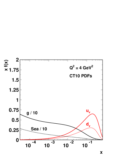
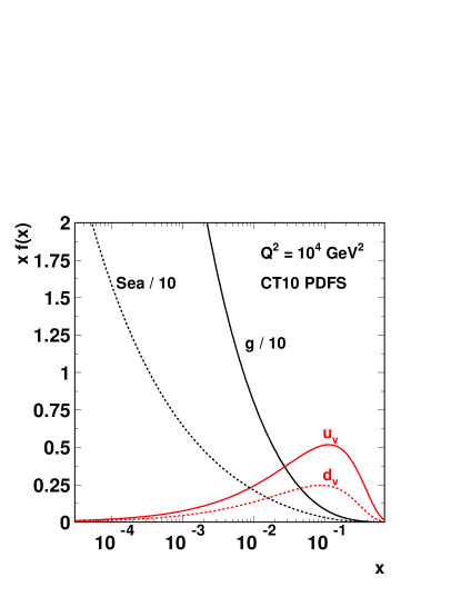
Figure 2: Example PDFs at NLO at $Q^{2}=4$ GeV² and $Q^{2}=10^{4}$ GeV²: the gluon density, the sea density $\sum\bar{q}$, and the valence densities $u_{v}=u-\bar{u}$ and $d_{v}=d-\bar{d}$.

The DGLAP equations allow the PDFs to be calculated perturbatively at any scale, once they have been measured at a given scale. Figure 2 shows example NLO PDFs for the gluon, the valence quarks and the sea quarks, for two values of $Q^{2}$. While the gluon and the sea distributions increase very quickly with $Q^{2}$, the non-singlet valence distributions are much less affected by the evolution.

Higher orders should also be accounted for in the partonic matrix element $\hat{\sigma}$ of Eq. 6, such that $\hat{\sigma}\rightarrow\hat{\sigma}_{0}+\hat{\sigma}_{1}(\mu_{F},\alpha_{s}(\mu_{R}))+...$. At LO in $\alpha_{s}$ the $\mu_{F}$ dependence can be absorbed into the PDFs but beyond LO this cannot be done in a process independent way, and hence $\hat{\sigma}$ depends on $\mu_{F}$ and on the factorisation scheme. An all orders calculation then cancels the $\mu_{F}$ dependence of the PDFs with the $\mu_{F}$ dependence of $\hat{\sigma}$. The factorisation scheme most commonly used is also the $\overline{\rm MS}$ scheme, and a common choice of factorisation and renormalisation scales is $\mu_{F}=\mu_{R}=Q$. It is conventional to estimate the influence of uncalculated higher order terms by varying both scales by factors of two.

At NLO the relationships between the structure functions (or any other scattering cross section) and the PDFs are modified in a factorisation scheme dependent way. The modifications are characterised by Wilson coefficient functions $C$ for the hard scattering process expressed as a perturbative series.

In the $\overline{\rm MS}$ scheme Eqs. 10 and 11 take additional corrections to the parton terms such that for $F_{2}$ the relation becomes, with the factorisation and renormalisation scales both set to $Q^{2}$ :

$$F_{2}(x,Q^{2}) = x\sum_{i}e_{i}^{2}q^{S}_{i}(x,Q^{2})+$$ (25)

$$\frac{\alpha_{s}(Q^{2})}{2\pi}x\int_{x}^{1}\frac{dy}{y}\left[\sum_{i}e_{i}^{2}C_{2,q}\left(\frac{x}{y}\right)q^{S}_{i}(y,Q^{2})+e^{2}_{i}C_{2,g}\left(\frac{x}{y}\right)g(y,Q^{2})\right]\,\,\,.$$

The $C_{2,q}$ and $C_{2,g}$ terms are the coefficient functions for $q$ induced and $g$ induced scattering contributing to $F_{2}$. Here the scaling violations are seen explicitly in the additional term proportional to $\alpha_{s}$ where the integrand is sensitive to partonic momentum fractions $y>x$. For low and medium $x$, the integral is dominated by the second term and $y\sim x$. Hence, from the scale dependence of $\alpha_{s}$, the derivative $\partial F_{2}/\partial\ln Q^{2}$, to the first order in $\ln Q^{2}$, is driven by the product of $\alpha_{s}$ and the gluon density. By replacing the $e_{i}^{2}$ couplings with the corresponding ones for $Z/\gamma^{*}$ interference and pure $Z$ exchange as in Eq. 10 the QCD corrected formulae for $F_{2}^{\gamma/Z}$ and $F^{Z}_{2}$ are obtained.

QCD corrections to $F_{L}$ and $xF_{3}$ must also be taken into account. For $xF_{3}$ the LO QCD corrected formula is

$$xF_{3}(x,Q^{2}) = x\sum_{i}q^{NS}_{i}(x,Q^{2})+\frac{\alpha_{s}(Q^{2})}{2\pi}x\int_{x}^{1}\frac{dy}{y}C_{3,q}\left(\frac{x}{y}\right)q^{NS}_{i}(y,Q^{2})\,\,,$$ (26)

and is independent of the $g$ density resulting in much weaker scaling violations than for $F_{2}$. Finally for $F_{L}$

$$F_{L}(x,Q^{2}) = \frac{\alpha_{s}(Q^{2})}{2\pi}x\int_{x}^{1}\frac{dy}{y}\left[\sum_{i}e_{i}^{2}C_{L,q}\left(\frac{x}{y}\right)q^{S}_{i}(y,Q^{2})+e^{2}_{i}C_{L,g}\left(\frac{x}{y}\right)g(y,Q^{2})\right]\,\,.$$ (27)

The coefficient functions at LO in the $\overline{\rm MS}$ scheme are given below for completeness

$$C_{2,q}(x) = \frac{4}{3}\left[\frac{1+x^{2}}{1-x}\left(\ln{\frac{1-x}{x}}-\frac{3}{4}\right)+\frac{1}{4}(9+5x)\right]_{+}$$

$$C_{2,g}(x) = n_{f}\left[(x^{2}+(1-x)^{2})\ln{\frac{1-x}{x}}-1+8x(1-x)\right]$$

$$C_{L,q}(x) = \frac{8}{3}x$$

$$C_{L,g}(x) = 4n_{f}x(1-x)$$

$$C_{3,q}(x) = C_{2,q}(x)-\frac{4}{3}(1+x)\,\,.$$ (28)

In the DIS scheme, $C_{2,q}(x)$ and $C_{2,g}(x)$ are zero.

To date an enormous variety of processes have been measured at colliders and confronted with the predictions of pQCD. These include not only inclusive measurements of DIS cross sections, but also semi-inclusive measurements of jet production rates, angular distributions, and multiplicities in DIS and in hadronic colliders as well as in $e^{+}e^{-}$ collisions. In all cases pQCD provides a good description of the measurements.

2 Experimental Constraints

In the following sections we describe the main features and results of experiments that put constraints on unpolarised proton PDFs. For reasons of space we do not provide a complete description of all experimental data, but rather focus on those experiments whose data is used in global approaches to extract the PDFs. The chapter naturally divides into common measurement techniques in DIS, measurements from fixed target DIS experiments, results from the HERA $ep$ collider which dominates the bulk of precision proton structure data, and results from hadro-production experiments. The LHC experiments will be described in chapter 4. A convenient online repository of experimental scattering data for PDF determinations can be found at [57]. A summary of the experimental constraints described here will be given in section 2.5 that concludes this chapter.

2.1 Measurement Techniques in DIS

The following sections outline some of the general issues faced by experimentalists in performing their measurements. These include corrections to the measured event rates to account for detector losses due to inefficiency and resolution effects, as well as theory-based corrections to extract structure functions and to take into account the sometimes large effects of QED radiation. Finally fixed target measurements are discussed which often require corrections for nuclear targets and kinematic effects that arise at low $Q^{2}$.

2.1.1 Detector efficiency and resolution corrections

Experimental corrections to account for the limited and imperfect detector acceptance are performed using Monte Carlo simulations but require an input PDF to be used. Thus the acceptance corrections are weakly dependent on these input PDFs. Experimenters circumvent this problem using an iterative approach whereby the measured structure functions are then further used to tune the MC input which leads to a modified measurement. The procedure is stopped when the iterations converge, i.e. the difference in the measurements changes by a small amount. Typically this occurs after one or two iterations [58].

2.1.2 Extraction of structure functions

The measured structure functions and differential cross sections are quoted at a point in $x$ and $Q^{2}$ and are derived from bin integrated values. A correction is needed to convert the measurement to a differential one. This is usually performed with a parameterisation of the cross section derivatives across the bin volume. This can be done by weighting each event by the ratio of structure functions at the bin centre and the $x$, $Q^{2}$ of that event [59]. Alternatively the bin integrated measurement can be corrected by a single factor which is the ratio of the structure function at the bin centre to the bin integrated value derived from an analytical calculation [60]. The dependence of the correction on the input parameterisation is usually small.

Early experiments often presented results as final corrected values of the electromagnetic structure functions $F_{2}$ and $F_{L}$ (or $R$). In order to make this decomposition of the cross section experimentalists restricted themselves to the phase space region of low $y$ where the contribution of $F_{L}$ is strongly suppressed in order to extract $F_{2}$. Alternatively a value of $F_{L}$ may be assumed in order to extract $F_{2}$. Both of these approaches have been used, but recent publications focus on the measurement of the differential cross section as the primary measurement which necessarily has fewer assumptions. Extractions of the individual structure functions are also provided for convenience. The H1 and ZEUS experiments recommend the use of differential cross sections only as input to further QCD analyses of the data [61].

By utilising different beam energies, scattering cross sections can be measured at fixed points in $x$ and $Q^{2}$ but different $y$ thus allowing direct measurements of the structure function $F_{L}$ to be made. Since the technique relies on the measurement of the difference between cross section measurements for two or more values of $\sqrt{s}$ the experimental uncertainties on $F_{L}$ are sensitive to systematic uncertainties in the relative normalisation of the data sets, and are often highly correlated point-to-point.

2.1.3 Reconstruction Methods

When the centre-of-mass energy of the interaction is known, the DIS cross section depends on two variables only, and the kinematic variables $x$, $y$ and $Q^{2}$ can be fully reconstructed from two independent measurements. Fixed target experiments of charged lepton DIS generally used the measurement of the energy and angle of the scattered lepton to reconstruct the kinematics - the lepton method.

The use of colliding beams to measure DIS cross sections allowed new detector designs to be employed whereby the HERA experiments could fully reconstruct the hadronic final state in most of the accessible kinematic domain. Hence, $x$, $y$ and $Q^{2}$ in NC interactions may be determined using energy and angular measurements of the scattered lepton alone, measurements of the inclusive hadronic final state (HFS), or some combination of these. This redundancy allows very good control of the measurements and of their systematic uncertainties. In contrast charged lepton CC interactions may only be reconstructed using measurements of the hadronic final state since the final state neutrino is unobserved. Each method has different experimental resolution and precision as well as different influence from QED radiative corrections (see below). A convenient summary of the different methods is given in [61] and are compared in [62].

At HERA the main NC reconstruction methods used are the double-angle method [63] (using the polar angles of the lepton and HFS), and the $e\Sigma$ method [64] which combines the scattered lepton energy and angle with the total energy and longitudinal momentum difference, $E-P_{Z}$, of the HFS.

DIS experiments using a (wide band) muon neutrino beam face an additional problem in determining the incident neutrino energy. It is usually reconstructed as the sum of the momentum of the scattered muon and of the energy of the HFS measured in a calorimeter. A third independent measurement, usually taken to be the angle of the scattered muon, is then needed to fully reconstruct the kinematics.

2.1.4 QED radiative corrections

The treatment of radiative corrections is an important aspect of DIS scattering cross sections measurements and was first discussed in [65]. The corrections allow measured data to be corrected back to the Born cross section in which the influence of real photon emission and virtual QED loops are removed. It is the Born cross sections that are then used in QCD analyses of DIS data to extract the proton PDFs (see section 3). This topic has been extensively discussed for HERA data in [66] and the references therein.

Corrections applied to the measured data are usually expressed as the ratio of the Born cross section to the radiative cross section and can have a strong kinematic dependence since for example, the emission of a hard real photon can significantly skew the observed lepton momentum. Thus the corrections also depend on the detailed experimental treatment and the choice of reconstruction method used to measure the kinematic quantities. In $ep$ scattering, hard final state QED radiation from the scattered electron is experimentally observable only at emission angles which are of the size of the detector spatial resolution.

Complete QED calculations at fixed order in $\alpha$ are involved and often approximations are used, particularly for soft collinear photon emission. These approximations are readily implemented into Monte Carlo simulations allowing experimentalists to account for radiative effects easily. For the HERA measurements [61] $\mathcal{O}(\alpha)$ diagrams are corrected for with the exception of real photon radiation off the quark lines. This is achieved using Monte Carlo implementations  [67, 68] checked against analytical calculations [48, 69] which agree to within  $0.3-1\%$ in the NC case ($2\%$ for $x>0.3$) and to within $2\%$ for the CC case. The quarkonic radiation piece is known to be small and is accounted for in the uncertainty given above.

The real corrections are dominated by emission from the lepton lines and are sizable at high and low $y$ [66]. For example, at $\sqrt{s}=301$ GeV and $Q=22~{}$GeV the leptonic $ep$ corrections are estimated to be $+40\%$ at $y=0.75$ when using the lepton reconstruction method. This is dramatically reduced to $+15\%$ if the $e\Sigma$ reconstruction method is used, and if an analysis cut of $E-P_{Z}>35$ GeV is employed the correction is further reduced to $+8\%$ [70].

The vacuum polarisation effects are also corrected for such that published cross sections correspond to $\alpha(Q\equiv 0)=1/137.04$. These photon self energy contributions depend only on $Q$ and amount to a correction of $-6\%$ for $Q=M_{Z}$ and $-4\%$ for $Q=12$ GeV.

2.1.5 Higher order weak corrections

The weak corrections are formally part of the complete set of $\mathcal{O}(\alpha)$ radiative corrections to DIS processes but are often experimentally treated separately to the QED radiative corrections discussed above. The weak parts include the self energy corrections, weak vertex corrections and so-called box diagrams in which two heavy gauge bosons are exchanged [66]. The self energy corrections depend on internal loops including all particles coupling to the gauge bosons e.g. the Higgs boson, the top quark and even new particle species. For this reason experimentalists sometimes publish measurements in which no corrections for higher order weak corrections are accounted for. Rather, comparisons to theoretical predictions are made in which the weak corrections are included in the calculations. Care must be taken to define the scheme (i.e. the set of input electroweak parameters used) within which the corrections are defined.

Two often used schemes are the on-mass-shell scheme [71], and the $G_{\mu}$ scheme [72]. In the former the EW parameters are all defined in terms of the on shell masses of the EW bosons. The weak mixing angle $\theta_{W}$ is then related to the weak boson masses by the relation $\sin^{2}{\theta_{W}}=1-M_{W}^{2}/M_{Z}^{2}$ to all perturbative orders. In the $G_{\mu}$ scheme, the Fermi constant which is very precisely known through the measurements of the muon lifetime [73], is used instead of $M_{W}$.

The scheme dependence is of particular importance in the CC scattering case where the influence of box diagrams is relatively small and the corrections are dominated by the self energy terms of the $W$ propagator affecting the normalisation of the cross section. In the $G_{\mu}$ scheme these leading contributions to the weak corrections are already absorbed in the measured value of $G_{\mu}$ and the remaining corrections are estimated to be at the level of $0.5\%$ at $Q^{2}=10\,000$ GeV² [74] where experimental uncertainties are an order of magnitude larger. For the HERA NC structure function measurements the EW corrections are estimated to reach the level of $\sim 3\%$ at the highest $Q^{2}$ [75] and should be properly accounted for in fits to the data.

2.1.6 Target mass corrections and higher twist corrections

For scattering processes at low scales approaching soft hadronic scales such as the target nucleon mass, additional hadronic effects lead to kinematic and dynamic $1/Q^{2}$ power corrections to the factorisation ansatz Eq. 6. Both of these corrections are important for DIS at low to moderate $Q^{2}$, in particular in the kinematic domain covered by fixed target DIS experiments.

In DIS, power corrections of kinematic origin, the target mass corrections (TMC), arise from the finite nucleon mass. For a mass $m_{N}$ of the target nucleon, the Bjorken $x$ variable is no longer equivalent to the fraction of the nucleon’s momentum carried by the interacting parton in the infinite momentum frame. This momentum fraction is instead given by the so-called Nachtmann variable $\xi$:

$$\xi=\frac{2x}{1+\gamma}\qquad{\mbox{ with }}\qquad\gamma=\sqrt{1+4x^{2}m_{N}^{2}/Q^{2}}$$

which differs from $x$ at large $x$ (above $\sim 0.5$) and low to moderate $Q^{2}$. Approximate formulae which relate the structure functions on a massive nucleon $F_{i}^{TMC}(x,Q^{2})$ to the massless limit structure functions $F_{i}$ can be found in [76, 77], for example:

$$F_{2}^{TMC}(x,Q^{2})=\frac{x^{2}}{\xi^{2}\gamma^{3}}F_{2}(\xi,Q^{2})+\frac{m_{N}^{2}}{Q^{2}}\frac{6x^{3}}{\gamma^{4}}\int_{\xi}^{1}d\xi^{\prime}/\xi^{\prime 2}F_{2}(\xi^{\prime},Q^{2})\qquad.$$

The ratios $F_{i}^{TMC}/F_{i}$ rise above unity at large $x$, with the rise beginning at larger values of $x$ as $Q^{2}$ increases. The target mass correction can be quite large: for $x=0.8$ it reaches $\sim 30\%$ at $Q^{2}=5$ GeV².

In addition, power corrections of dynamic origin, arising from correlations of the partons within the nucleon, can also be important at low $Q^{2}$. The contribution of these higher twist terms [78] to the experimentally measured structure functions $F_{i}^{exp}$ can be written as

$$F_{i}^{exp}(x,Q^{2})=F_{i}^{TMC}(x,Q^{2})+H_{i}(x)/Q^{2}+...$$ (29)

These terms have been studied in [79] and more recently in [80, 81] and found to be sizable at large $x$, however they remain poorly known. QCD analyses of proton structure that make use of low $Q^{2}$ data may impose kinematic cuts to exclude the measurements made at low $Q^{2}$ and high $x$ (i.e. at low $W^{2}$) that may be affected by these higher twist corrections. Alternatively, a model can be used for the $H_{i}(x)$ terms, whose parameters can be adjusted to the data.

2.1.7 Treatment of data taken with a nuclear target

Neutrino DIS experiments have used high $Z,A$ targets such as iron or lead, which provide reasonable event rates despite the low $\nu$ interaction cross section. The expression of the measured quantities, $F_{2}^{A}$, in terms of the proton parton densities, has to account for the facts that:

• the target is not perfectly isoscalar; e.g. in iron, there is a $6.8\%$ excess of neutrons over protons;

• nuclear matter modifies the parton distribution functions; i.e. the parton distributions in a proton bound within a nucleus of mass number $A$, $f^{A}(x,Q^{2})$, differ from the proton PDF $f(x,Q^{2})$. Physical mechanisms of these nuclear modifications (shadowing effect at low $x$, the nucleon’s Fermi motion at high $x$, nuclear binding effects at medium $x$) are summarised e.g. in [83, 84]. The ratios $R^{A}=f^{A}(x,Q^{2})/f(x,Q^{2})$ are called nuclear corrections, and can differ from unity by as much as $10-20\%$ in medium-size nuclei.

Nuclear corrections are obtained by dedicated groups, from fits to data of experiments that used nuclear ($A$) and deuterium ($d$) targets: the structure function ratios $F_{2}^{A}/F_{2}^{d}$ measured in DIS (at SLAC by E139, and at CERN by the EMC and NMC experiments), and the ratios of Drell-Yan $q\bar{q}$ annihilation cross sections $\sigma_{DY}^{A}/\sigma_{DY}^{d}$ measured by the E772, E866 experiments. Recent analyses also include the measurements of inclusive pion production obtained by the RHIC experiments in deuterium-gold collisions at the Brookhaven National Laboratory (BNL). The measurements of charged current DIS structure functions at experiments using a neutrino beam (see sections 2.2.4 and 2.2.6) can also be included, as done in [85] for example.

Figure 3 shows an example of nuclear corrections for the $u_{v}$, $\bar{u}$, $\bar{s}$ and $g$ densities at a scale of $Q^{2}=10$ GeV², as obtained from the recent analysis described in [85]. They are shown for beryllium ($A=9$), iron ($A=56$), gold ($A=197$) and for lead ($A=208$). The size of the nuclear corrections is larger for heavier nuclei. Nuclear effects in deuterium are usually neglected, although some QCD analyses [81] account for them explicitly. They were studied in [86] by analysing data on $F_{2}^{d}/F_{2}^{p}$ and were found to be small, ${\cal{O}}(1-2)\%$. In [81] nuclear corrections on $F_{2}^{d}$ were found to be below $2\%$ for $x<0.7$, rising above $10\%$ for $x>0.8$.

Nuclear corrections derived from other analyses are also overlaid in Fig. 3. While the correction factors obtained by these analyses are in reasonable agreement for the up and down quarks, sizable differences are observed for other flavours and for the gluon.

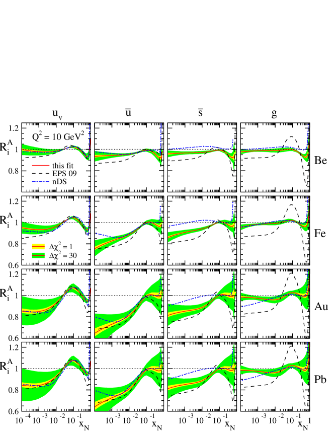
Figure 3: Example of nuclear corrections obtained from the analysis of [85], at $Q^{2}=10$ GeV², for four different nuclei. From [85].

Concerns have been raised in [87, 88, 89], regarding the possibility that nuclear corrections may be different for NC and CC DIS. Such a breaking of factorisation, if true, would cast serious doubts on the constraints on proton PDFs derived from neutrino DIS experiments. However, this was not confirmed by the recent analysis described in [85]. The analysis of [90] also reported no tension between the NC and CC DIS data off heavy nuclei.

2.2 Measurements from fixed target DIS experiments

A brief description of the main fixed target DIS experiments is given in this section. Further details can also be found in [91]. The $x$, $Q^{2}$ ranges and beam energies of the measurements are summarised in Tab. 1 in section 2.5. This latter section also contains a representative compilation of the measurements described here (see Fig. 15 and Fig. 16).

2.2.1 SLAC

The first experiments to probe the region of deep inelastic scattering were conducted by a collaboration between the Stanford Linear Accelerator group, the Massachusetts Institute of Technology, and the California Institute of Technology. The experiments used an electron linac capable of accelerating electrons up to $20$ GeV and a momentum analysing spectrometer arm equipped with scintillator hodoscopes and multi-wire proportional chambers (MWPCs) for electron detection, triggering and background rejection. The experiments were performed in the period 1970 to 1985 using one of three spectrometer arms selecting scattered electron momenta up to $1.6$, $8$, and $20$ GeV. All three were mounted on a common pivot around the target area and able to measure different scattering angles. The spectrometers were designed to decouple the measurement of scattering angle of the electron and its momentum. This was achieved by careful design of the spectrometer optics in which dipole and focusing quadrupole magnets were used to deflect electrons in the vertical plane depending on momentum, and causing horizontal dispersion of the electrons depending on the scattering angle.

The major experiments relevant to QCD analyses of proton structure are E49a/b, E61, E87, E89a/b, E139 and E140. In total some $6,000$ data points were measured for $ep$ and $ed$ scattering. The latter two high statistics experiments used the $8$ GeV spectrometer, with a $30^{\circ}$ vertical bend to deflect scattered electrons into the detector assembly region.

Using improved methods of applying radiative corrections, and better knowledge of $R$ [92], the SLAC data were re-evaluated with a more rigorous error treatment yielding smaller uncertainties for the relative normalisations between the individual experiments. A final summary dataset of all SLAC experiments combined with precise determinations of $F_{2}^{p}$ and $F_{2}^{d}$ were published [93, 94]. This combined data set achieved a typical $3$% statistical uncertainty, and similar systematic uncertainties. The measurements cover a region extending to high $x$, $0.06\leq x\leq 0.9$, and $0.6\leq Q^{2}\leq 30$ GeV². Despite their very good precision, the measurements at highest $x$ are usually not included in QCD analyses because higher twist effects are important in the domain where they were made (see section 3.2.1).

2.2.2 BCDMS

The BCDMS experiment [95] was a collaboration between the research institutes of Bologna, CERN, Dubna, Munich and Saclay, formed in 1978 and utilised the CERN SPS M2 muon beam with energies of $100$, $120$, $200$, $280$ GeV. The experiment was designed to enable precise measurements of $R$ to be made with tight control of systematic uncertainties using the high intensity muon beam. The intense beam spills placed stringent requirements on the experimental trigger and background rejection abilities. The experiment collected high statistics data on proton and deuteron targets [97, 96]. The targets were located serially along the common axis of eight iron toroid modules, with each module consisting of scintillator hodoscopes and MWPCs.

The primary measurements were the inclusive double differential cross sections corrected for radiative effects and presented as $F_{2}(x,Q^{2})$. Measurements of the total inclusive cross section at different centre of mass energies allowed $R$ to be determined. The data cover the region $0.06\leq x\leq 0.8$ and $7\leq Q^{2}\leq 260$ GeV². The final measured values of $F_{2}$ have a typical statistical precision of $1-2\%$ and a similar systematic uncertainty, which at high $x$ reaches up to $5\%$ arising from the spectrometer field calibration and resolution.

The BCDMS data provide a precise measurement of the $F_{2}$ structure function in the valence region of high $x$. The $R$ data show similar $x$ dependence of the two polarised pieces of the cross section at high $x$, but indicate an increasing longitudinal component at low $x$ consistent with the expectation of an increasing gluon component of the proton.

2.2.3 NMC

The New Muon Collaboration (NMC) was a muon scattering DIS experiment at CERN that collected data from $1986-1989$ using the M2 muon beam line from the CERN SPS. It was designed to measure structure function ratios with high precision.

The experimental apparatus [98] consisted of an upstream beam momentum station and hodoscopes, a downstream beam calibration spectrometer, a target region and a muon spectrometer. The muon beam ran at beam energies of $90,120,200,$ and $280$ GeV. The muon beams illuminated two target cells containing liquid hydrogen and liquid deuterium placed in series along the beam axis. Since the spectrometer acceptance was very different for both targets they were regularly alternated. The muon spectrometer was surrounded by several MWPCs and drift chambers to allow a full reconstruction of the interaction vertex and the scattered muon trajectory. Muons were identified using drift chambers placed behind a thick iron absorber.

The experiment published measurements of the proton and deuteron differential cross sections $d^{2}\sigma/dxdQ^{2}$ in the region $0.008<x<0.5$ and $0.8<Q^{2}<65$ GeV², from which the structure functions $F_{2}^{p}$ and $F_{2}^{d}$ were extracted [58]. A statistical precision of $~{}2\%$ across a broad region of the accessible phase space was achieved, and a systematic precision of between $2$ and $5\%$. NMC have also published direct measurements of $R(x,Q^{2})$ in the range $0.0045<x<0.11$ [58] which provides input to the gluon momentum distribution.

In addition the collaboration published precise measurements of the ratio $F_{2}^{d}/F_{2}^{p}$ [99] which is sensitive to the ratio of quark momentum densities $d/u$. By measuring the ratio of structure functions several sources of systematic uncertainty cancel including those arising from detector acceptance effects and normalisation. Thus measurements in regions of small detector acceptance could be performed and these cover the region $0.001<x<0.8$ and $0.1<Q^{2}<145$ GeV² with a typical systematic uncertainty of better than $1\%$. The ratio $F_{2}^{d}/F_{2}^{p}$ was seen to decrease as $x\rightarrow 1$, indicating that $d(x)$ falls more quickly than $u(x)$ at high $x$; the behaviour of $d/u$ as $x$ approaches $1$ remains however unclear.

In 1992 NMC published the first data on the Gottfried sum rule[100] which in the simple quark parton model states that $\int_{0}^{1}\frac{dx}{x}F_{2}^{p}-F_{2}^{n}=\frac{1}{3}\int_{0}^{1}dx(u_{v}-d_{v})+\frac{2}{3}\int_{0}^{1}dx(\bar{u}-\bar{d})\,\,,$ and assuming $\bar{u}-\bar{d}=0$, should take on a value of $\frac{1}{3}$. The initial NMC measurement indicated a violation of this assumption of a flavour symmetric sea. This was verified by the final NMC analysis[101] in which the Gottfried sum was determined to be $0.235\pm 0.026$ at $Q^{2}=4$ GeV², which implies that $\int dx(\bar{d}-\bar{u})\sim 0.15$, indicating a significant excess of $\bar{d}$ over $\bar{u}$.

2.2.4 CCFR/NuTeV

The Chicago-Columbia-Fermilab-Rochester detector (CCFR) was constructed at Fermilab to study DIS in neutrino induced lepton beams on an almost isoscalar iron target. The detector used the wide band mixed $\nu_{\mu}$ and $\bar{\nu}_{\mu}$ beam reaching energies of up to $600$ GeV. The CCFR experiment collected data in 1985 (experiment E744) and in 1987-88 (E770).

In 1996 the NuTeV experiment (E815), using the same detector, was used in a high statistics neutrino run with the primary aim of making a precision measurement of $\sin^{2}{\theta_{W}}$. The major difference between NuTeV and its predecessor CCFR was ability to select $\nu_{\mu}$ or ${\bar{\nu}}_{\mu}$ beams which also limited the upper energy of the wide band beam to $\simeq~{}500$ GeV. The neutrino beam was alternated every minute with calibration beams of electrons and hadrons throughout the one year data taking period. This allowed a precise calibration of the detector energy scales and response functions to be obtained.

The neutrino beam was produced by protons interacting with a beryllium target. Secondary pions and kaons were sign selected and focused into a decay volume. The detector was placed $1.4$ km downstream of the target region and consisted of a calorimeter composed of square steel plates interspersed with drift chambers and liquid scintillator counters. A toroidal iron spectrometer downstream of the calorimeter provided the muon momentum measurement using a $1.5$ T magnetic field. In total NuTeV logged $3\cdot 10^{18}$ protons on target.

Structure function measurements

CCFR published measurements of $F_{2}$ and $xF_{3}$  [102] with a typical precision of $2-3$% on $F_{2}$ which is largely dominated by the statistical uncertainty on the data. The data cover the region $0.015\leq x\leq 0.65$ and $1.26\leq Q^{2}\leq 126$ GeV². As discussed in 1.3, these measurements are a direct test of the total valence density. NuTeV measured the double differential cross sections $d^{2}\sigma/dxdy$ from which the structure functions $F_{2}$ and $xF_{3}$ were determined [103, 104, 105] from linear fits to the neutrino and anti-neutrino cross section data. The data generally show good agreement between the two experiments and the earlier low statistics CDHSW experiment [106]. However, at $x>0.4$ an increasing systematic discrepancy between CCFR and NuTeV was observed. A mis-calibration of the magnetic field map of the toroid in CCFR explains a large part of this discrepancy [103], and the NuTeV measurements are now believed to be more reliable.

Semi-inclusive di-muon production

In addition to providing inclusive cross section measurements, both experiments also measured the semi-inclusive $\mu^{+}\mu^{-}$ production cross section, in $\nu_{\mu}-$ and $\bar{\nu}_{\mu}-$nucleon interactions [107]. Such di-muon events arise predominantly from charged-current interactions off a strange quark, with the outgoing charmed meson undergoing a semi-leptonic decay, as illustrated in Fig. 4. These measurements thus provide a direct constraint on the strange quark density in the range $0.01<x<0.4$.

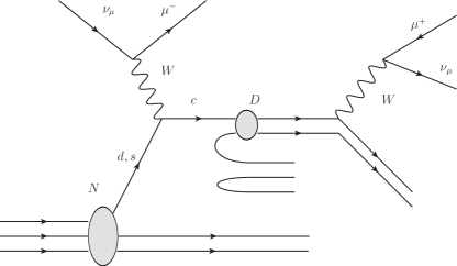
Figure 4: Exclusive di-muon production in $\nu_{\mu}$ deep inelastic scattering.

Moreover, the separation into $\nu_{\mu}$ and $\bar{\nu}_{\mu}$ cross sections allows a separation of the $s$ and $\bar{s}$ contributions to be made, since di-muon events are mainly produced from $W^{+}s\rightarrow c\rightarrow\mu^{+}+X$ with an incoming $\nu_{\mu}$ beam, or from $W^{-}\bar{s}\rightarrow\bar{c}\rightarrow\mu^{-}+X$ with a $\bar{\nu}_{\mu}$ beam. These data favour a non-vanishing asymmetry $s-\bar{s}$, as discussed further in section 3.5.5.

2.2.5 E665

This muon scattering experiment at Fermilab operated from $1987-1992$ measuring deep inelastic scattering of muons off proton and deuteron targets in regularly alternating target cells  [59]. The data cover the range $0.0009<x<0.4$ and $0.2<Q^{2}<64$ GeV².

The experiment consisted of a beam spectrometer, target region and main spectrometer. The beam spectrometer was designed to detect and reconstruct the beam muon momentum using trigger hodoscopes, multi-wire proportional chambers and a dipole magnet. The target region consisted of cells filled with liquid hydrogen and liquid deuterium placed in a field free region and which were alternated regularly. The main spectrometer was located immediately downstream of the target region and consisted of two large dipole magnets with reversed polarity. A series of drift and multi-wire proportional chambers placed inside and downstream of both magnets provided comprehensive tracking coverage. Further downstream a lead-gas sampling electromagnetic calorimeter was placed in front of iron absorbers followed by the muon detectors consisting of planes of proportional tubes and trigger hodoscopes.

The measurements of $F_{p}^{p}$ and $F_{2}^{d}$ typically have statistical uncertainties of $6$% and $5$% respectively and systematic uncertainties of better than $4$%. The E665 $\mu p$ and $\mu d$ data partially overlap with measurements from NMC at higher $Q^{2}$. The $x$ range of E665 data overlaps with that covered by the HERA experiments H1 and ZEUS (see section 2.3) though these data on $F_{2}^{p}$ lie at higher values of $Q^{2}$. Comparisons between the experiments show good agreement between NMC and E665, and the HERA data show a smooth continuous evolution for fixed $x$ with increasing $Q^{2}$.

2.2.6 CHORUS

The CERN Hybrid Oscillation Research ApparatUS (CHORUS) [108] was originally a $\nu_{\mu}\rightarrow\nu_{\tau}$ appearance experiment in operation at CERN from 1994-1997 [109]. In 1998 the run was exclusively used for differential measurements of neutrino induced CC DIS using the lead-scintillator calorimeter as an active target [110] as well as studying the $Z/A$ dependence of the total CC cross section [111]. The experiment utilised the $450$ GeV proton beam from the SPS which was directed to a target producing charged particles. These were sign selected and focused into a decay volume followed by iron and earth to filter out the neutrinos which emerged with a wide energy range $10<E_{\nu}<200$ GeV. The detector consisted of a lead-fibre scintillator calorimeter with nine planes of modules with alternating orientation in the plane transverse to the beam. The muon spectrometer was made of six toroidal iron magnets interspersed with drift chambers scintillators and streamer tubes to reconstruct the muon momentum.

The differential cross sections in $x$, $y$ and $E_{\nu}$ are measured in the range $0.02\leq x\leq 0.65$ and in $0.3\leq Q^{2}\leq 82$ GeV². These are used to extract the structure functions $F_{2}$ and $xF_{3}$ in a linear fit to the $y$ dependence of the cross sections for each $x,Q^{2}$ bin. The statistical uncertainty on $F_{2}$ is in the region of $1\%$ and the systematic contribution to the uncertainty is typically below $3\%$ for $x>0.1$ and increases at lower $x$. The data for $xF_{3}$ are in agreement with earlier measurements from CCFR [112] and the hydrogen target neutrino experiment CDHSW [106]. The $F_{2}$ measurements are in better agreement with those from CCFR than with NuTeV.

2.3 The H1 and ZEUS experiments

The HERA collider was the first colliding beam $ep$ accelerator operating at centre-of-mass energies of $301$ and later at $319$ GeV. At the end of the operating cycle two short low energy runs at $\sqrt{s}=225$ and $250$ GeV were taken for a dedicated $F_{L}$ measurement. At the highest centre of mass energy the beams had energies of $920$ GeV for the protons and $27.6$ GeV for the electrons. The two experiments utilising both HERA beams were H1 and ZEUS and they provide the bulk of the precision DIS structure function data over a wide kinematic region. In particular, HERA opened up the domain of $x$ below a few $10^{-3}$ which had been mostly unexplored by the fixed target experiments. The fixed target experiments HERMES and HERA-B will not be discussed in this article.

The accelerator operation is divided into three periods or datasets: HERA-I from 1992 to 2000, HERA-II from 2003 to 2007, and the dedicated Low Energy Runs taken in 2007 after which the accelerator was decommissioned. During the 2001-2003 upgrade of the accelerator and the experiments, spin rotators were installed in the lepton beam line allowing longitudinally polarised lepton beam data to be collected, with a polarisation of up to $\pm 40$%. In total H1 and ZEUS together collected almost $1$ fb^-1 of data evenly split between lepton charges and polarisations.

A review of the physics results of the H1 and ZEUS experiments can be found in [113], and the HERA structure function results have been recently reviewed in [114].

2.3.1 Experimental Apparatus

The two experiments were designed as general purpose detectors, nearly $4\pi$ hermetic, to analyse the full range of $ep$ physics with well controlled systematic uncertainties. The highly boosted proton beam led to asymmetric detector designs with more hadronic instrumentation in the forward (proton) direction which had to withstand high rates and high occupancies.

The most significant differences between them are the calorimeters, which had an inner electromagnetic section and an outer hadronic part. ZEUS employed a compensating Uranium scintillator calorimeter located outside the solenoidal magnet providing a homogeneous field of $1.4$ T. H1 used a lead/steel liquid argon sampling calorimeter located in a cryostat within the solenoid field of $1.16$ T and a lead/scintillating fibre backward electromagnetic calorimeter for detection of scattered leptons in neutral current processes. In both H1 and ZEUS, a muon detector was surrounding the calorimeter.

Both experiments utilised drift chambers in the central regions for charged particle detection and momentum measurements which were enhanced by the installation of precision silicon trackers. They allowed the momenta and polar angles $\theta$ of charged particles to be measured in the range of $7^{\circ}<\theta<165^{\circ}$, the backward region of large $\theta$ being where the scattered electron was detected in low $Q^{2}$ NC DIS events. In H1 an additional drift chamber gave access to larger angles of up to $\sim 172^{\circ}$.

2.3.2 Neutral Current measurements from H1 and ZEUS

Figure 5 (left) shows the spread in parameterisations of $F_{2}$ which existed prior to the first HERA data. Most extrapolations from pre-HERA data indicated a “flattish” $F_{2}$ at low $x$ - which was also expected from Regge-like arguments. The first HERA results [115, 116] presented in $1993$ were based on $30$ nb^-1 of data taken in $1992$ and showed a surprising, strong rise of $F_{2}$ towards low $x$. An example [115] of these measurements is shown in Fig. 5 (centre). With the full HERA-I dataset, the statistical uncertainty of these low $x$ and low $Q^{2}$ measurements could be reduced below $1\%$, with a systematic error of about $2\%$; the measurements are shown in Fig. 5 (right).

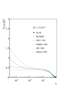
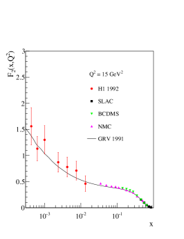
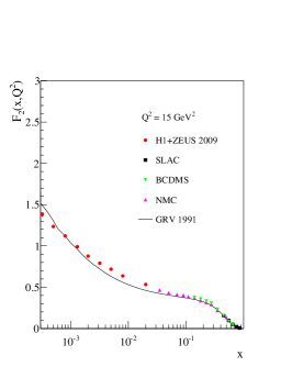
Figure 5: Left: the spread of the theoretical predictions for $F_{2}$ which were consistent with pre-HERA data for $Q^{2}=15$ GeV². Centre: The first $F_{2}$ measurements from H1 in 1992. Right: The complete HERA-I measurements of $F_{2}$.

With increasing luminosity, high statistics were accumulated over the whole kinematic domain [61]. Fig. 15 in the summary section 2.5 shows an overview of HERA $F_{2}$ measurements together with data points from fixed target experiments. The very strong scaling violations are clearly observed at low $x$. This indicates a large gluon density since at leading order $\partial F_{2}/\partial\ln Q^{2}$ is driven at low $x$ by the product of $\alpha_{s}$ and the gluon density $g(x,Q^{2})$ (see Eq. 25). At high $x$ the scaling violations are negative: high $x$ quarks split into a gluon and a lower $x$ quark. The curves overlaid are the result of QCD fits (see section 3) based on the DGLAP evolution equations. The data show an excellent agreement with DGLAP predictions, over five orders of magnitude in $Q^{2}$ and four orders of magnitude in $x$.

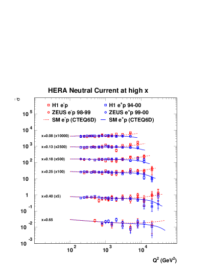
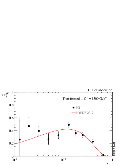
Figure 6: Left: The NC DIS cross section as a function of $Q^{2}$ for several values of $x$, measured in $e^{+}p$ (blue symbols) and in $e^{-}p$ (red symbols) collisions. The Standard Model predictions are overlaid, as the full and dashed curves, respectively. Right: The structure function $xF^{\gamma Z}_{3}$ extracted from the complete H1 HERA-I+II dataset. From [75, 122].

At very high $Q^{2}$, the NC cross sections are sensitive to the $Z$-exchange, resulting in $\sigma_{NC}(e^{-}p)\neq\sigma_{NC}(e^{+}p)$ as was seen in Sec. 1.3. The NC cross sections have been measured at high $Q^{2}$ both in $e^{+}p$ and in $e^{-}p$ collisions [117, 118, 75, 119, 120, 121, 122], as shown in Fig. 6. The contribution of $Z$ exchange is clearly visible for $Q^{2}$ above about $10^{3}$ GeV², with the $\gamma-Z$ interference being constructive (destructive) in $e^{-}p$ ( $e^{+}p$) collisions. The difference between both measurements gives access to the structure function $x\tilde{F}_{3}$ which is a direct measure of the valence quark distributions (see Eqs. 7 and 11). The H1 measurement using the full HERA-II luminosity [122] is shown in Fig. 6 (right).

HERA collider operation concluded with data taking runs at two reduced proton beam energies in order to facilitate a direct measurement of $F_{L}$. This structure function gives a larger contribution to the cross section with increasing $y$ (see Eq. 7). It can therefore be determined by measuring the differential cross section at different $\sqrt{s}$, i.e. at the same $x$ and $Q^{2}$ but different $y$. Measurements from H1 and ZEUS have been published [123, 124] covering the low $x$ region of $3\times 10^{-5}-10^{-2}$ and $Q^{2}$ from $1.5-120$ GeV².

2.3.3 Charged Current DIS measurements

Measurements of charged current DIS provide important constraints on the flavour separation, which are missing from the measurement of $F_{2}$ alone, as the latter mostly constrains one single combination of PDFs ($4U+D$). Indeed (see Eq. 12 and Eq. 13-14), $\sigma^{-}_{CC}$ goes as $(1-y)^{2}x\bar{D}+xU$ and probes mainly the $u$ density, while $\sigma^{+}_{CC}$ goes as $(1-y)^{2}xD+x\bar{U}$ and probes mainly the $d$ density, with some constraints being also set on $\bar{U}$ via the high $y$ measurements. An example of CC measurements is shown in Fig. 7. Although the statistical precision of the HERA-II CC measurements [122, 125, 126] is much better than what was achieved with HERA-I [127, 128], these measurements remain statistically limited. For example, the precision reaches $\sim 10\%$ for $x\sim 0.1$.

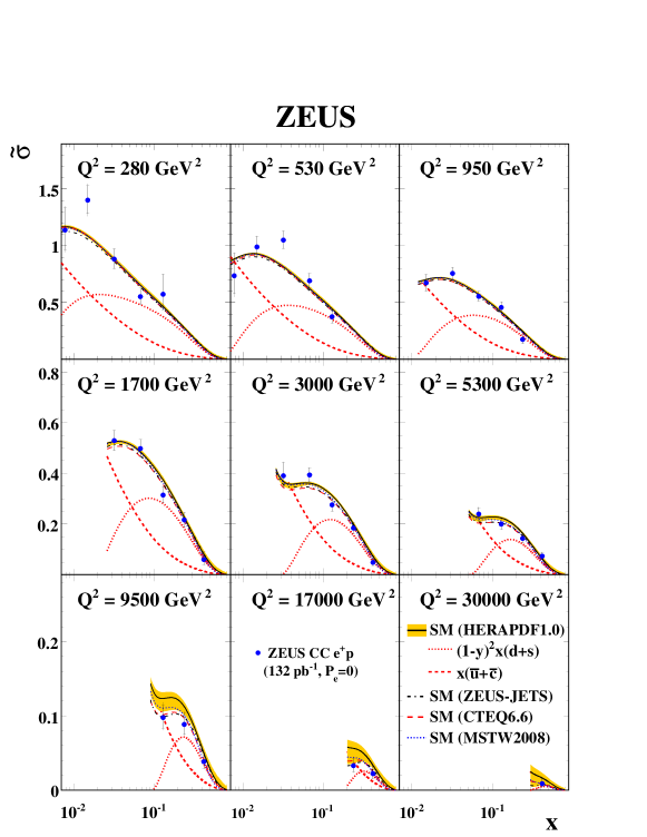
Figure 7: The CC DIS cross section measured in $e^{+}p$ collisions. The overlaid curves show how these measurements disentangle the contributions from up and down quarks. From [126].

Despite this moderate precision, the constraints brought by CC DIS at HERA are interesting since the experimental input is completely free of any correction, in contrast to those obtained by comparing DIS measurements on a proton and a deuterium target.

2.3.4 The averaged H1 and ZEUS DIS dataset

Recently the two collaborations have embarked on a programme of data combination leading to joint publications of combined data which profit from improved uncertainties over the individual measurements. A novel, model independent, statistical method has been employed, which was introduced in [129] and further refined in [130]. By taking into account the variations of the measurements arising from different experimental sources of uncertainty an improvement in the statistical and systematic uncertainties is obtained. This arises from the fact that each experiment uses different methods of measurement and each method can act as a calibration of the other.

The unique assumption of the averaging method is that both experiments measure the same quantity or cross section at a given $x$ and $Q^{2}$. The averaging procedure is based on the minimisation of a $\chi^{2}$ function with respect to the physical cross sections in all $(x,Q^{2})$ bins of the measurement. Each experimental systematic error source is assigned a nuisance parameter with a corresponding penalty term in the $\chi^{2}$ function to restrict large deviations of the parameter from zero. These parameters induce coherent shifts of the measured cross sections according to the correlated systematic uncertainties provided by the experiments. The distribution of the fitted nuisance parameters in an ideal case should be Gaussian distributed with a mean of zero and variance of one.

Several types of cross section measurement can be combined simultaneously e.g. NC $e^{+}p$, NC $e^{-}p$, CC $e^{+}p$ and CC $e^{-}p$, yielding four independent datasets all of which benefit from a reduction in the uncertainty. In this case the reduction arises from correlated sources of uncertainty common to all cross section types. This data combination method has been described in detail and used in several publications [130, 60, 61].

This procedure also has the advantage of producing a single set of combined data for each cross section type which makes analysis of the data in QCD fits practically much easier to handle. The first such combination of H1 and ZEUS inclusive neutral and charged current cross sections has been published using HERA-I data [61]. Further combination updates are expected to follow as final cross sections using HERA-II data are published by the individual experiments.

As an example Fig. 8 shows the neutral current cross section for unpolarised $e^{+}p$ scattering. The combined data are shown compared to the individual H1 and ZEUS measurements. The overall measurement uncertainties are reduced at high $x$ mainly from improved statistical uncertainties. However at low $x$ where the data precision is largely limited by systematic uncertainties, a clear improvement is also visible. In the region of $Q^{2}\sim 30$ GeV² the overall precision on the combined NC cross sections has reached $1.1$% [61]. In the CC $e^{+}p$ channel the measurement accuracy is limited by the statistical sample sizes and the combined data reduces the uncertainty to about $10\%$ for $x\sim 0.1$. A further significant reduction in uncertainty is expected once the combination of H1 and ZEUS data including the complete HERA-II datasets is available.

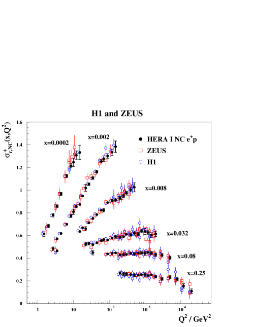
Figure 8: HERA combined NC $e^{+}p$ reduced cross section as a function of $Q^{2}$ for six $x-$bins, compared to the separate H1 and ZEUS data input to the averaging procedure. The individual measurements are displaced horizontally for better visibility. From [61].

The combined HERA datasets have been used in QCD analyses [61] to determine proton PDFs with HERA data alone. This is described in more detail in section 3.4.1.

2.3.5 Heavy flavour measurements: $\boldsymbol{F_{2}^{c\bar{c}}}$ and $\boldsymbol{F_{2}^{b\bar{b}}}$

The charm and beauty contents of the proton have been measured at HERA via exclusive measurements (exploiting

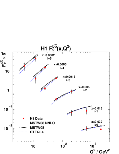
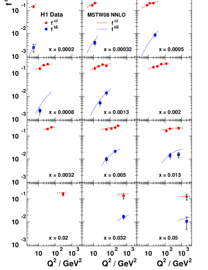
Figure 9: Left: $F_{2}^{b{\bar{b}}}$ measured by the H1 experiment using a lifetime technique. Right: the fractions of charm and beauty in the proton, derived from the same analysis. From [135].

for example the $D^{*}\rightarrow D^{0}\pi_{\rm{slow}}\rightarrow K\pi\pi$ decay chain, or the $b\rightarrow\mu X$ decays, see e.g. [131, 132, 133, 134]), and via semi-inclusive measurements which exploit the long lifetime of the charmed and beauty hadrons, using silicon vertex devices around the interaction points [135, 136]. Figure 9 (left) shows the $F_{2}^{b\bar{b}}$ measured by the H1 experiment [135]. Just as for the inclusive $F_{2}$, it shows large scaling violations at low $x$. In Fig. 9 (right), the charm fraction in the proton is shown to be about $20\%$ independently of $Q^{2}$, while the beauty fraction increases rapidly with $Q^{2}$, reaching $\sim 1\%$ at high $Q^{2}$. The precision of the measurements of $F_{2}^{c\bar{c}}$ and $F_{2}^{b\bar{b}}$ is about $\sim 15\%$ and $\sim 30\%$, respectively. These measurements provide an important test of the theoretical schemes within which observables involving heavy flavours are calculated (see section 3.2.2).

2.3.6 Dedicated measurements at very low $\boldsymbol{Q^{2}}$

Extending the $F_{2}$ measurements down to very low $Q^{2}$ requires dedicated techniques or detectors. The squared momentum transfer $Q^{2}$ can be written as $Q^{2}=2E^{0}_{e}E_{e}(1+\cos\theta_{e})$, where $E^{0}_{e}$ denotes the energy of the incoming lepton in the laboratory frame, $E_{e}$ that of the scattered lepton, and $\theta_{e}$ is the angle of the scattered lepton with respect to the direction of the incoming proton. Thus it can be seen by inspection that to go down to low $Q^{2}$, one needs to access larger angles $\theta_{e}$, or to lower the incoming electron energy $E^{0}_{e}$. This can be achieved by:

• using a dedicated apparatus, as the ZEUS Beam Pipe Tracker (BPT), which consisted of a silicon strip tracking detector and an electromagnetic calorimeter very close to the beam pipe in the backward electron direction;

• shifting the interaction vertex in the forward direction. Two short runs were taken with such a setting, where the nominal interaction point was shifted by $70$ cm;

• exploiting QED Compton events: when the lepton is scattered at a large angle $\theta_{e}$, it may still lead to an observable electron (i.e. within the detector acceptance) if it radiates a photon.

• using events with initial state photon radiation which can lower the incoming electron energy $E^{0}_{e}\rightarrow E^{0}_{e}-E_{\gamma}$ where $E_{\gamma}$ is the energy of the radiated photon.

All these methods have been exploited at HERA [137]. In particular, it was observed that $F_{2}$ continues to rise at low $x$, even at the lowest $Q^{2}$, $Q^{2}\sim 0.5$ GeV². Note that these measurements are usually not included in QCD analyses determining parton distribution functions, since they fail the lower cut in $Q^{2}$ that is usually applied to DIS measurements, to ensure that they are not affected by non-perturbative effects.

2.3.7 Jet cross sections in DIS at HERA

The H1 and ZEUS experiments have measured inclusive jet cross sections in the so-called “Breit” frame as a function of several variables, for example differentially with respect to the jet energy and in several $Q^{2}$ bins [138, 139, 140, 141, 142]. The Breit frame [143] is of particular interest for jet measurements at HERA since it provides a maximal separation between the products of the beam fragmentation and the hard jets. In this frame, the exchanged virtual boson $V^{*}$ is purely space-like and is collinear with the incoming parton, with $\vec{q}=(0,0,-Q)$. For parton-model processes, $V^{*}q\rightarrow q$, the virtual boson is absorbed by the struck quark, which is back-scattered with zero transverse momentum with respect to the $V^{*}$ direction. On the other hand, for $\mathcal{O}(\alpha_{s})$ processes like QCD-Compton scattering ($V^{*}q\rightarrow qg$) and boson-gluon fusion ($V^{*}g\rightarrow q\bar{q}$), the two final-state partons lead to jets with a non-vanishing transverse momentum. Hence, the inclusive requirement of at least one jet in the Breit frame with a high transverse momentum selects $O(\alpha_{s})$ processes and suppresses parton-model processes. Example measurements of inclusive jet production in DIS obtained by the ZEUS experiment are shown in Fig. 10. With small systematic uncertainties of typically $\sim 5\%$, such data can bring constraints on the gluon density in the medium $x$ range, $x=0.01-0.1$. However, when included in global QCD fits which also include other jet data, the impact of these measurements is limited [38].

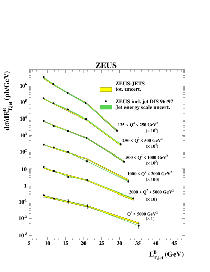
Figure 10: Differential cross sections of inclusive jet production in DIS measured by the ZEUS experiment, together with their systematic uncertainties. From [142].

Jet production has also been measured in the photoproduction regime of $Q^{2}\rightarrow 0$. However, these measurements are usually not included in QCD analyses of the proton structure because of their potential sensitivity to the photon parton densities.

2.4 Experiments with hadronic beams

In interactions where no lepton is involved in the initial state, the cross sections depend on products of parton distribution functions as shown by Eq. 6. Hadro-production experiments, using either a fixed target or two colliding beams, provide a wealth of measurements that nicely complement those made in lepto-production. In particular, they set specific constraints on some parton distribution functions that are not directly accessed in DIS experiments. The corresponding measurements, performed by fixed target experiments and by the D0 and CDF experiments at the Tevatron collider, are described in this section.

2.4.1 Kinematics in hadro-production

In $pp$, $pd$ or $p\bar{p}$ collisions, the production of a final state of invariant mass $M$ involves two partons with Bjorken-$x$ values $x_{1}$ and $x_{2}$ related by

$$M^{2}=x_{1}x_{2}s$$ (30)

where $s$ denotes the square of the energy in the centre of mass of the hadronic collision. The minimum value of $x_{1,2}$ is thus $x_{min}=\tau$ with

$$\tau\equiv M^{2}/s$$ (31)

In the rest frame of the two hadrons and neglecting the hadron masses, the rapidity $y$ of the final state $X$ is

$$y=\frac{1}{2}\ln\frac{E-p_{z}}{E+p_{z}}=\frac{1}{2}\ln\frac{x_{1}}{x_{2}}$$ (32)

where the hadron that leads to the parton with momentum fraction $x_{1}$ defines the positive direction along the beam(s) axis. Hence $x_{1}$ and $x_{2}$ can be written as

$$x_{1}=\sqrt{\tau}e^{y}\qquad,\qquad x_{2}=\sqrt{\tau}e^{-y}$$ (33)

In fixed target experiments, the positive direction is usually defined by the direction of the incident beam, such that $x_{1}$ denotes the Bjorken-$x$ of the parton in the beam hadron, and $x_{2}$ that of the parton in the target hadron. In $p\bar{p}$ collisions, the positive direction can be defined by the proton beam, in which case $x_{1}$ ($x_{2}$) denotes the Bjorken-$x$ of the parton in the proton (anti-proton).

2.4.2 Drell-Yan di-muon production in fixed target experiments

The experiments E605, E772 and E866/NuSea have measured di-muon production in Drell-Yan interactions of a proton off a fixed target. They used an $800$ GeV proton beam extracted from the Fermilab Tevatron accelerator that was transported to the east beamline of the Meson experimental hall. While changes were made to the spectrometer for E772 and E866/NuSea, the basic design has remained the same since the spectrometer was first used for E605 in the early 1980s. The core consists of three large dipole magnets that allow the momentum of energetic muons to be measured and deflect soft particles out of the acceptance. Different targets have been employed: copper for E605, liquid deuterium for E772 and E866, and liquid hydrogen for E866. The centre-of-mass energy of the Drell-Yan process for these experiments is $\sqrt{s}=38$ GeV. A broad range of di-lepton invariant mass $M$ could be covered, extending up to $M\sim 20$ GeV.

Differential cross sections

The experiments published [144, 145] double-differential cross sections in $M$ and either in the rapidity of the di-lepton pair $y$, or in Feynman $x_{F}$, defined as $x_{F}=2q_{z}/\sqrt{s}$ where $q$ denotes the four-vector of the Drell-Yan pair in the hadronic centre-of-mass frame and $q_{z}$ its projection on the longitudinal axis. At leading order, $x_{F}=x_{1}-x_{2}$ and the leading order differential cross sections can be written as:

$$\frac{d^{2}\sigma}{dM^{2}dy} = \frac{4\pi\alpha^{2}}{9M^{2}s}\sum_{i}e^{2}_{i}\left[q_{i}(x_{1})\bar{q}_{i}(x_{2})+\bar{q}_{i}(x_{1})q_{i}(x_{2})\right]$$ (34)

$$\frac{d^{2}\sigma}{dM^{2}dx_{F}} = \frac{1}{x_{1}+x_{2}}\frac{d\sigma}{dM^{2}dy}\qquad.$$ (35)

The experiments made measurements in the range $4.5<M<14$ GeV and $0.02<x_{F}<0.75$, corresponding to $x_{1}\sim 0.1-0.8$ and $x_{2}\sim 0.01-0.3$, the acceptance of the detector being larger for $x_{1}\gg x_{2}$. In this domain, the first term dominates in Eq. 34, and the measurements bring important information on the sea densities $\bar{u}(x)$ and $\bar{d}(x)$, especially for $x$ larger than about $0.1$ where DIS experiments poorly constrain the sea densities.

The ratio $\boldsymbol{pp/pd}$ from E866

E866/NuSea made measurements using both a deuterium and a hydrogen target [146, 147, 148] from which ratios of the differential cross sections $\sigma_{pp}/\sigma_{pd}$ could be extracted. These measurements have brought an important insight on the asymmetry $\bar{d}-\bar{u}$ at low $x$. Indeed, the cross sections in the phase space where $x_{1}\gg x_{2}$ can be written as:

$$\sigma_{pp} \propto \frac{4}{9}u(x_{1})\bar{u}(x_{2})+\frac{1}{9}d(x_{1})\bar{d}(x_{2}),\qquad$$ (36)

$$\sigma_{pn} \propto \frac{4}{9}u(x_{1})\bar{d}(x_{2})+\frac{1}{9}d(x_{1})\bar{u}(x_{2})$$ (37)

such that:

$$\frac{\sigma_{pd}}{2\sigma_{pp}}\sim\frac{1}{2}\frac{1+\frac{1}{4}\frac{d(x_{1})}{u(x_{1})}}{1+\frac{1}{4}\frac{d(x_{1})}{u(x_{1})}\frac{\bar{d}(x_{2})}{\bar{u}(x_{2})}}\left[1+\frac{\bar{d}(x_{2})}{\bar{u}(x_{2})}\right].$$

In the relevant domain of $x_{1}$, the ratio $d(x_{1})/u(x_{1})$ is quite well known, such that the ratio $\sigma_{pd}/2\sigma_{pp}$ gives access to the ratio $\bar{d}/\bar{u}$ at low and medium $x$, $x\sim 0.01-0.3$.

This idea was first used by the NA51 experiment at CERN [149], which confirmed the indication, previously obtained by the NMC experiment, that $\bar{d}\neq\bar{u}$ (see section 2.2.3). But the acceptance of the NA51 detector was limited, and their result for $\bar{d}/\bar{u}$ ($\bar{d}/\bar{u}\sim 2$) could be given for a single $x$ value only.

The E866 experiment was the first to measure the $x$-dependence of $\bar{d}/\bar{u}$. Fig. 11 shows the obtained measurement [147], which extends down to $x_{2}\sim 0.03$. Note the spread of the theoretical predictions before these data were included in the fits. The ratio $\bar{d}/\bar{u}$ as extracted by E866 is shown in Fig. 11 (right), and clearly demonstrates that $\bar{d}>\bar{u}$. The asymmetry between $\bar{d}$ and $\bar{u}$ is largest for $x\sim 0.2$ and decreases with decreasing $x$; what happens as $x\rightarrow 1$ remains unclear.

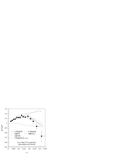
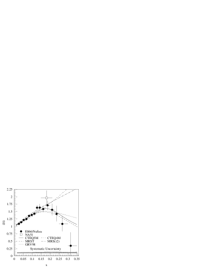
Figure 11: Left: The ratio $\sigma_{pd}/2\sigma_{pp}$ measured by the E866 experiment. Right: The ratio $\bar{d}/\bar{u}$ extracted from this measurement. The previous result from the NA51 experiment is also shown as the open square. From [147].

2.4.3 The D0 and CDF experiments at Fermilab

The D0 and CDF experiments were located at the Tevatron collider at Fermilab, which collided protons and anti-protons. In a first phase of operation (“Run I”, from $1992$ to $1998$), the Tevatron was operated at a centre-of-mass energy of $1.8$ TeV. The second phase, “Run II”, started in $2001$ following significant upgrades of the accelerator complex and of the experiments, with a centre-of-mass energy of $1.96$ TeV. The data taking has stopped in $2011$.

The measurements of the D0 and CDF experiments provide several important constraints on proton structure:

• measurements of lepton charge asymmetry from $W$ decays bring constraints on the ratio $d/u$ at $x>0.05$, and hence on the $d$ density, which is less well known than the $u$ density;

• measurements of the $Z$ rapidity distribution in $Z\rightarrow l^{+}l^{-}$ decays bring constraints on the quark densities at $x>0.05$, which are complementary to those obtained from DIS measurements;

• the cross sections for inclusive jet production in several rapidity bins provide constraints on the gluon and the quark distributions for $0.01<x<0.5$. In particular, they set the strongest constraints on the gluon density at high $x$.

A detailed description of the D0 detector can be found in [150]. The inner most part is a central tracking system surrounded by a $2$ T superconducting solenoidal magnet. The two components of the central tracking system, a silicon microstrip tracker and a central fibre tracker, are used to reconstruct interaction vertices and provide the measurement of the momentum of charged particles in the pseudo-rapidity range $\mid\eta\mid<2$. The tracking system and magnet are followed by the calorimetry system that consists of electromagnetic and hadronic uranium-liquid argon sampling calorimeters. Outside of the D0 calorimeter lies a muon system which consists of layers of drift tubes and scintillation counters and a 1.8 T toroidal magnet.

The CDF II detector is described in detail in [151]. The detector has a charged particle tracking system that is immersed in a $1.4$ T solenoidal magnetic field coaxial with the beam line, and provides coverage in the pseudo-rapidity range $\mid\eta\mid<2$. Segmented sampling calorimeters, arranged in a projective tower geometry, surround the tracking system and measure the energy of interacting particles for $\mid\eta\mid<3.6$.

Lepton charge asymmetry from $\boldsymbol{W}$ decays

In $pp$ or $p\bar{p}$ collisions, the production of $W^{+}$ bosons proceeds mainly via $u\bar{d}$ interactions, or via $\bar{u}d$ for $W^{-}$ production. At large boson rapidity $y_{W}$, the interaction involves one parton with $x=\sqrt{\tau}\exp{|y_{W}|}$ (see Eq. 33) where $\sqrt{\tau}=M_{W}/\sqrt{s}\sim 0.04$. In $p\bar{p}$ collisions at the Tevatron, this medium to high $x$ parton is most likely to be a $u$ quark picked up from the proton in the case of $W^{+}$ production, or a $\bar{u}$ anti-quark from the anti-proton in $W^{-}$ production; this follows from the fact that $u(x)>d(x)$ at medium and high $x$. Hence, $W^{+}$ bosons are preferably emitted in the direction of the incoming proton and $W^{-}$ bosons in the anti-proton direction, leading to an asymmetry between the rapidity distributions of $W^{+}$ and $W^{-}$ bosons. This asymmetry can be written as:

$$A(y_{W}) = \frac{d\sigma(W^{+})/dy_{W}-d\sigma(W^{-})/dy_{W}}{d\sigma(W^{+})/dy_{W}+d\sigma(W^{-})/dy_{W}}$$ (38)

$$\sim \frac{u(x_{1})d(x_{2})-d(x_{1})u(x_{2})}{u(x_{1})d(x_{2})+d(x_{1})u(x_{2})}$$ (39)

$$= \frac{R(x_{2})-R(x_{1})}{R(x_{2})+R(x_{1})}\sim y_{W}\sqrt{\tau}R^{\prime}(\sqrt{\tau})/R(\sqrt{\tau})$$ (40)

where $R(x)=d(x)/u(x)$ and $R^{\prime}$ denotes the derivative of $R$. It can be seen from Eq. 40 that the $W$ charge asymmetry is directly sensitive to the $d/u$ ratio in the range $x\sim 0.01-0.3$, and to its slope at $x\sim 0.04$.

This asymmetry remains, though diluted, when measuring the experimentally observable rapidity of the charged lepton coming from the $W$ decay [153, 154, 155, 156]. Figure 12 shows example measurements from the CDF experiment, in two bins of the transverse energy $E_{T}$ of the lepton. At low $E_{T}$, the measured asymmetry is also sensitive to the anti-quark densities, via subleading interactions involving an anti-quark coming from the proton and a quark from the anti-proton, which were neglected in the approximate formula Eq. 40.

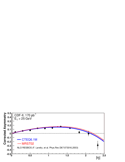
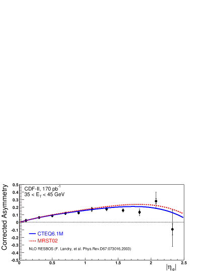
Figure 12: Lepton charge asymmetry from $W$ decays, as a function of the pseudo-rapidity of the charged lepton. The asymmetry is shown for two ranges of the lepton transverse energy. From [154].

Rapidity distribution in $\boldsymbol{Z\rightarrow l^{+}l^{-}}$ events

The large integrated luminosity delivered by the Tevatron allows the $Z$ rapidity distribution to be precisely measured by the D0 and CDF experiments [157, 158]. The $Z/\gamma^{*}$ rapidity distribution is measured in a di-lepton mass range around the $Z$ boson mass, extending up to $\mid y\mid\sim 3$. The measurements provide constraints on the quark densities at $Q^{2}\sim M^{2}_{Z}$, over a broad range in $x$. Neglecting the $Z/\gamma^{*}$ interference terms, which are small in the considered mass range and well below the experimental uncertainties, the differential cross section reads as:

$$\frac{d\sigma}{dy} = \frac{\pi G_{F}M^{2}_{Z}\sqrt{2}}{3s}\sum_{i}c_{i}\left[q_{i}(x_{1})\bar{q}_{i}(x_{2})+\bar{q}_{i}(x_{1})q(x_{2})\right]$$ (41)

where $c_{i}=v_{i}^{2}+a_{i}^{2}$ is the sum of the squares of the vector and axial couplings of the quarks to the $Z$ boson. Hence, the measured cross sections mainly probe the combination

$$\sim 0.29u(x_{1})u(x_{2})+0.37d(x_{1})d(x_{2})\quad{\rm{with}}\quad x_{1,2}=\frac{M_{Z}}{\sqrt{s}}e^{\pm y}$$ (42)

complementary to the combination $\sim 4u\bar{u}+d\bar{d}$ probed by $pp$ Drell-Yan production in fixed target experiments (see section 2.4.2 and Eq. 36). These D0 and CDF measurements bring interesting constraints on the $d$ distribution and, in the forward region, on the quark densities at high $x$.

Inclusive jet cross sections

The Tevatron measurement of the jet production cross section with respect to the jet transverse momentum $p_{T}$, $d^{2}\sigma/dp_{T}dy$, in several bins of jet rapidity $y$, provide constraints on the quark and gluon densities for $x$ larger than a few $10^{-2}$. For example, in the central rapidity region, the production of jets with $p_{T}=200$ GeV involves partons with $x\simeq 0.2$, and at least one of them is a gluon in $\sim 70\%$ of interactions. Hence, these measurements provide crucial constraints on the gluon density at high $x$.

The jet measurements from Run I [159, 160] preferred a rather high gluon density at high $x$, in some tension with the other experimental measurements available at that time, as discussed in section 3.5.4. As will be seen in section 3, this tension is much reduced with the Run II measurements [161, 162, 163, 164]. An example of these measurements, from the D0 collaboration, is shown in Fig. 13.

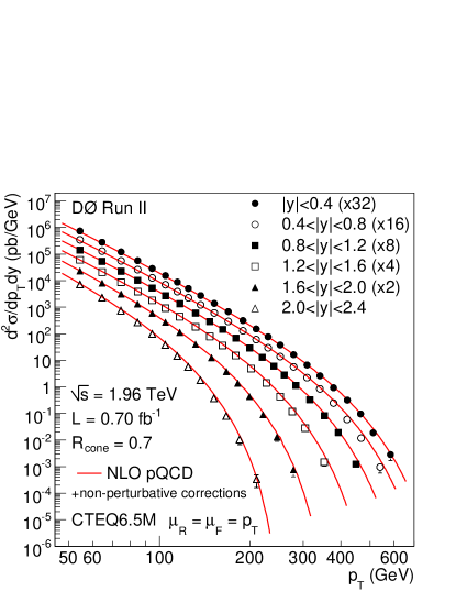
Figure 13: Inclusive jet cross section as a function of jet $p_{T}$, as measured by the D0 experiment. From [162].

These measurements are presented in six bins of jet rapidity extending out to $\mid y\mid=2.4$. The cross section extends over more than eight orders of magnitude from $p_{T}=50$ GeV to $p_{T}>600$ GeV. Compared to previous Run I results, the systematic uncertainties have been reduced by up to a factor of two, to typically $\sim 10-15\%$. This has been made possible by extensive studies of the jet response, which lead to a relative uncertainty of the jet $p_{T}$ calibration of about $1\%$ for jets measured in the central calorimeter, for $p_{T}$ in $150-500$ GeV.

2.4.4 Prompt photon production

In hadronic interactions, the production of prompt photons, i.e. photons that do not arise from the decay of a hadron produced in the interaction, is sensitive to the gluon density via the QCD Compton process $qg\rightarrow\gamma q$. However, measurements of inclusive prompt photon production performed at low energy ($\sqrt{s}=20-40$ GeV) by the fixed target E706 experiment [165, 166, 167] could not easily be included in QCD analyses of proton PDFs, as they were systematically higher than theoretical predictions [168, 169]. Consequently, once precise jet measurements from the Tevatron experiments became available, they were used instead of the prompt photon data to constrain the gluon density at medium and high $x$, and the usage of prompt photon measurements in QCD fits was abandoned.

Since then, the compatibility of prompt photon measurements with pQCD predictions has been discussed at length, and the current status is reviewed in [170]. With respect to older measurements, measurements performed in hadronic collisions, at higher $\sqrt{s}$, are less affected by non-perturbative effects such as intrinsic $k_{T}$ broadening [166, 171]. Moreover, the requirement that the photon be isolated reduces the contribution of photons coming from fragmentation processes. These fragmentation photons are less well understood and are subject to large uncertainties. The analysis performed in [170] considered the measurements of isolated prompt photon production carried out by:

• the Tevatron experiments, at $\sqrt{s}=0.63-1.96$ TeV; photons with a transverse energy between $7$ and $400$ GeV were measured, corresponding to a range in $x$ of $10^{-3}$ to $0.4$;

• the UA1 experiment at the CERN Sp$\bar{{\rm{p}}}$S, at $\sqrt{s}=0.55-0.63$ TeV; photons of $12$ to $100$ GeV were measured, covering a range of $0.01$ to $0.5$ in $x$;

• the PHENIX experiment at the RHIC collider at the Brookhaven National Laboratory. RHIC is the only collider than can collide polarised protons, as well as several species of heavy ions such as gold or uranium. In [172], unpolarised $pp$ cross sections were reported at $\sqrt{s}=200$ GeV, by averaging over the spin states of the proton beams, for the production of photons of $3$ to $16$ GeV, corresponding to a range in $x$ of $0.03$ to $0.2$.

Generally a good agreement with NLO pQCD predictions has been found. However, these data are not included in the QCD fits described in section 3.5.

2.5 Summary

The complete range of measurements used in proton structure determinations now span six orders of magnitude in both $x$ and $Q^{2}$ and is shown in Fig. 14. The region of high $x$ and low $Q^{2}$ is covered by the fixed target data with charged lepton and neutrino DIS experiments as well as proton beams on nuclear targets. The large $\sqrt{s}$ of the HERA collider provides access to a wide kinematic range. Finally the range of the Tevatron $p\bar{p}$ collider data operating at $\sqrt{s}=1.96$ TeV is shown providing access to $Q^{2}\sim 10^{5}$ GeV² through the inclusive jet measurements. A summary of the main features of the experimental measurements is provided in Tab. 1.

The PDF flavour decomposition of the proton is achieved by combining data from different types of experiment each of which brings its own constraints and are summarised in Tab. 2. The fixed target charged lepton DIS data provide stringent constraints on the light quark PDFs in the valence region of $x>0.1$ as well as medium $x\simeq 0.01$. The combination of $F_{2}$ measurements in NC DIS off a proton and a deuterium target provides the primary $U$-type and $D$-type flavour separation. For example the $F_{2}^{p}/F_{2}^{d}$ ratio of DIS inclusive measurements from NMC constrains the ratio of $u/d$ in a rather wide $x$ domain. Measurements of Drell-Yan di-muon production data are sensitive to the combination $q\bar{q}$ which at high $x$ constrains the anti-quarks. Neutrino induced DIS structure functions from CCFR, NuTeV and CHORUS disentangle the contribution of sea quarks from that of valence quarks, through the measurements of the CC structure functions $W_{2}$ and $xW_{3}$ at $x>0.01$. The di-muon production measurements allow the $s$ and $\bar{s}$ components to be ascertained via the process $\nu N\rightarrow\mu^{+}\mu^{-}+X$ (and the charge conjugate reaction) mediated by $W+s$ and $W+\bar{s}$ fusion.

The fixed target data generally benefit from large event rates in the high $x$ region but can be complicated by the use of nuclear targets. The HERA DIS data are not affected by these issues and the NC measurements place tight constraints on the low $x$ gluon distribution as well as the sea quark PDFs at low $x$. The CC measurements have moderate statistical precision but provide sufficient flavour separation to allow PDF extractions using only HERA data.

The existing measurements of $F_{2}$ are summarised in Fig. 15; it demonstrates the scaling violations which are most prominent at low $x$. The charged lepton $xF_{3}$ data are consistent albeit within large uncertainties as shown in Fig. 16. The neutrino induced DIS measurements also shown have much greater precision. Direct measurements of the $F_{L}$ structure function are also shown in Fig. 16. The precise fixed target data at high $x$ are compared to the HERA measurements lying at much lower $x$ with much larger uncertainties. There is good overall consistency of the variety of measurements from different experiments. The compatibility between the various experimental datasets is further discussed in section 3.5.6.

Combinations of the experimental observables listed here allow flavour separated PDFs of the proton to be extracted in pQCD analyses, as discussed in chapter 3.

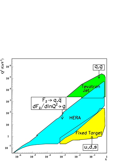
Figure 14: The kinematic plane in $(x,Q^{2})$ accessed by the DIS and hadron collider experiments. From [73].

Experiment		Measurement	$x_{min}$	$x_{max}$	$Q^{2}_{min}$	$Q^{2}_{max}$	ref.	Beam Energy
					(GeV2)	(GeV2)		(GeV)
SLAC	$ep$, $ed$	$F_{2}^{p}$, $F_{2}^{d}$	$0.06$	$0.9$	$0.6$	$30$	[93, 94]	$4-20$
SLAC	$ep$, $ed$	$R^{p}$, $R^{d}$	$0.1$	$0.9$	$0.6$	$20$	[92]	$4-17$
BCDMS	$\mu p$, $\mu d$	$F_{2}^{p}$, $F_{2}^{d}$	$0.07$	$0.8$	$7.5$	$230$	[97, 96]	$100$, $120$, $200$, $280$
BCDMS	$\mu p$, $\mu d$	$R^{p}$, $R^{d}$	$0.07$	$0.7$	$15$	$50$	[97, 96]	$100$, $120$, $200$, $280$
NMC	$\mu p$, $\mu d$	$F_{2}^{p}$, $F_{2}^{d}$	$0.008$	$0.5$	$0.8$	$65$	[58]	$90$, $120$, $200$, $280$
NMC	$\mu p$, $\mu d$	$R^{p}$, $R^{d}$	$0.0045$	$0.11$	$1.4$	$21$	[58]	$90$,$120$, $200$, $280$
NMC	$\mu p$, $\mu d$	$F_{2}^{p}/F_{2}^{d}$	$0.002$	$0.7$	$0.2$	$100$	[99]	$90$,$120$, $200$, $280$
E665	$\mu p$, $\mu d$	$F_{2}^{p}$, $F_{2}^{d}$	$0.0009$	$0.4$	$0.2$	$64$	[59]	$470$
HERA								$\sqrt{s}$ (GeV)
H1/ZEUS	$ep$	$\tilde{\sigma}_{NC},\tilde{\sigma}_{CC}$	$10^{-5}$	$0.65$	$0.1$	$30\,000$	[61]	$301,319$
H1/ZEUS	$ep$	$F_{L}$	$0.00003$	$0.01$	$1.5$	$120$	[123, 124]	$225,250$
Neutrino Experiments								Beam Energy (GeV)
CCFR	$\nu_{\mu}Fe/\bar{\nu}_{\mu}Fe$	$F_{2}$, $xF^{\nu}_{3}$	$0.015$	$0.65$	$1.2$	$126$	[102]	$30-500$
NuTeV	$\nu_{\mu}Fe/\bar{\nu}_{\mu}Fe$	$F_{2}$,$xF^{\nu}_{3}-xF^{\bar{\nu}}_{3}$	$0.015$	$0.75$	$1.2$	$125$	[103, 104, 105]	$30-360$
CCFR&NuTeV	$\nu_{\mu}Fe/\bar{\nu}_{\mu}Fe$	$\nu N/\bar{\nu}N\rightarrow\mu^{+}\mu^{-}X$	$0.02$	$0.36$	$1.2$	$117$	[107]	$30-500$
CHORUS	$\nu_{\mu}Pb/\bar{\nu}_{\mu}Pb$	$F_{2}$,$xF_{3}$	$0.02$	$0.65$	$0.3$	$82$	[110]	$30-360$
Hadron Beam Experiments								$\sqrt{s}$ (GeV)
E605	$pCu$	$\sigma_{pN}$	$0.14$	$0.65$	$51$	$286$	[144]	$800$
E772	$pd$	$\sigma_{pN}$	$0.026$	$0.56$	$23$	$218$	[145]	$800$
E866/NuSea	$pp/pd$	$\sigma_{pp}/\sigma_{pd}$	$0.026$	$0.56$	$21$	$166$	[147]	$800$
CDF/D0	$p\bar{p}$	$\sigma_{W,Z}$ , $Y_{Z}$, $A(Y_{W})$	$\sim 0.003$	$\sim 0.8$	$M_{W}^{2}$	$M_{Z}^{2}$	[157, 158, 152]	$1800,1960$
CDF/D0	$p\bar{p}$	$p\bar{p}\rightarrow$ incl. jets	$\sim 0.003$	$\sim 0.8$	$0.1$	$\sim 10^{5}$	[161, 162]	$1800,1960$

Table 1: Table of datasets generally used in current QCD fits. The kinematic range of each measurement in $x$ and $Q^{2}$ and the incident beam energy are also given. The normalisation uncertainties of the charged lepton scattering experiments are typically $2-3\%$.

Process	Subprocess	Partons	$x$ range
$\ell^{\pm}\,\{p,n\}\to\ell^{\pm}\,X$	$\gamma^{*}q\to q$	$q,\bar{q},g$	$x\gtrsim 0.01$
$\ell^{\pm}\,n/p\to\ell^{\pm}\,X$	$\gamma^{*}\,d/u\to d/u$	$d/u$	$x\gtrsim 0.01$
$pp\to\mu^{+}\mu^{-}\,X$	$u\bar{u},d\bar{d}\to\gamma^{*}$	$\bar{q}$	$0.015\lesssim x\lesssim 0.35$
$pn/pp\to\mu^{+}\mu^{-}\,X$	$(u\bar{d})/(u\bar{u})\to\gamma^{*}$	$\bar{d}/\bar{u}$	$0.015\lesssim x\lesssim 0.35$
$\nu(\bar{\nu})\,N\to\mu^{-}(\mu^{+})\,X$	$W^{*}q\to q^{\prime}$	$q,\bar{q}$	$0.01\lesssim x\lesssim 0.5$
$\nu\,N\to\mu^{-}\mu^{+}\,X$	$W^{*}s\to c$	$s$	$0.01\lesssim x\lesssim 0.2$
$\bar{\nu}\,N\to\mu^{+}\mu^{-}\,X$	$W^{*}\bar{s}\to\bar{c}$	$\bar{s}$	$0.01\lesssim x\lesssim 0.2$
$e^{\pm}\,p\to e^{\pm}\,X$	$\gamma^{*}q\to q$	$g,q,\bar{q}$	$0.0001\lesssim x\lesssim 0.1$
$e^{+}\,p\to\bar{\nu}\,X$	$W^{+}\,\{d,s\}\to\{u,c\}$	$d,s$	$x\gtrsim 0.01$
$e^{\pm}p\to e^{\pm}\,c\bar{c}\,X$	$\gamma^{*}c\to c$, $\gamma^{*}g\to c\bar{c}$	$c$, $g$	$0.0001\lesssim x\lesssim 0.01$
$e^{\pm}p\to\text{jet}+X$	$\gamma^{*}g\to q\bar{q}$	$g$	$0.01\lesssim x\lesssim 0.1$
$p\bar{p}\to\text{jet}+X$	$gg,qg,qq\to 2j$	$g,q$	$0.01\lesssim x\lesssim 0.5$
$p\bar{p}\to(W^{\pm}\to\ell^{\pm}\nu)\,X$	$ud\to W,\bar{u}\bar{d}\to W$	$u,d,\bar{u},\bar{d}$	$x\gtrsim 0.05$
$p\bar{p}\to(Z\to\ell^{+}\ell^{-})\,X$	$uu,dd\to Z$	$d$	$x\gtrsim 0.05$

Table 2: The main processes included in current global PDF analyses ordered in three groups: fixed target experiments, HERA and the Tevatron. For each process an indication of their dominant partonic subprocesses, the primary partons which are probed and the approximate range of $x$ constrained by the data is given. From [173].

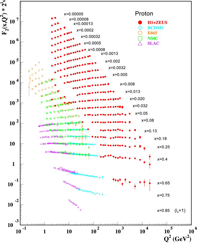
Figure 15: The proton structure function $F_{2}(x,Q^{2})$ measured in a wide kinematic range by various DIS experiments. From [73].

Figure 16: The proton structure functions $xF_{3}(x,Q^{2})$ and $F_{L}(x,Q^{2})$. From [73].

3 Determination of parton distribution functions

3.1 Introduction and generalities

Parton distribution functions are determined from fits of perturbative QCD calculations, based on the DGLAP evolution equations, to various sets of experimental data. These fits are regularly updated to account for new experimental input and theoretical developments. Most fits are performed at NLO, although leading order fits are still of interest, for example for Monte-Carlo simulations. With the recent, full calculation of the DIS cross section at NNLO [55], first NNLO fits are becoming available (see section 3.6).

In the following, we will discuss in particular the latest NLO fits performed by the CTEQ/CT group (CTEQ6.6 [174] and CT10 [175]), the MSTW group (MSTW08 [173]) and the NNPDF collaboration (NNPDF2.0 [176] and NNPDF2.1 [177]), which try to include all relevant experimental data. Other groups, e.g. GJR [178] or ABKM/ABM [81, 179, 180], also provide fits using a subset of data. The H1 and ZEUS collaborations have also published QCD fits based on their inclusive DIS data only (see e.g. HERAPDF1.0 [61]). The main differences between these various fits are described in the next sections. These fits are publicly available via the LHAPDF interface [181], which also provides access to older proton PDF fits as well as to photon and pion PDFs.

The general ansatz used in QCD fits is the parameterisation of parton distributions at a so-called starting scale $Q^{2}_{0}$, using a flexible analytic form. For example, one can choose to parameterise the gluon density $xg(x)$, the valence quark densities $xu_{v}(x)=x(u(x)-\bar{u}(x))$ and $xd_{v}(x)=x(d(x)-\bar{d}(x))$, the light sea distribution defined as $xS(x)=x\left[2(\bar{u}(x)+\bar{d}(x))+s(x)+\bar{s}(x)\right]$, and $x\Delta(x)\equiv x(\bar{d}(x)-\bar{u}(x))$. Most QCD analyses make use of a simple functional form, like:

$$xf_{i}(x,Q^{2}_{0})=A_{i}x^{\alpha_{i}}(1-x)^{\beta_{i}}P_{i}(x)$$ (43)

where $P_{i}(x)$ can be e.g. a polynomial function in $x$ or $\sqrt{x}$. The parameterisation can also be based on interpolation polynomials or non-linear functions. The latter approach is exploited by the NNPDF collaboration and is described in section 3.2.3 in more detail.

The DGLAP evolution equations are used to obtain, from these parameterised densities at $Q^{2}_{0}$, the parton densities $xf(x,Q^{2})$ at any $Q^{2}$. This allows the theoretical cross sections of the processes of interest (DIS, Drell-Yan di-lepton production, jet production, …) to be computed. The parameters that define the PDFs at the starting scale (e.g. $\alpha_{i}$, $\beta_{i}$, .. in Eq. 43) can then be obtained by fitting these theoretical predictions to the experimental measurements.

This is achieved by minimising a $\chi^{2}$ function. A usual choice for this function is:

$$\chi^{2}=\sum_{exp}\chi^{2}_{exp}$$ (44)

where the individual contribution of each independent dataset is given by [182, 183]:

$$\chi^{2}_{exp}=\sum_{i}\frac{(d_{i}-\sum_{k}\beta_{k,i}s_{k}-t_{i})^{2}}{\alpha_{i}^{2}}+\sum_{k}s^{2}_{k}\qquad.$$ (45)

In this equation,

• $d_{i}$ denote the measurements and $t_{i}$ the corresponding theoretical predictions;

• the total uncorrelated uncertainty affecting the measurement $i$ is given by $\alpha_{i}$ which sums in quadrature the statistical and the uncorrelated systematic uncertainties;

• $k$ labels the sources of correlated systematic uncertainties;

• $\beta_{k,i}$ is the amount of change of $d_{i}$ when the source $k$ (for example an energy scale) is shifted by one standard deviation ($s_{k}=1$); the values of $\beta_{k,i}$ are taken from the correlated systematic error tables published by the experiments;

• the second term in Eq. 45 introduces a quadratic penalty $s_{k}^{2}$ when the data points are moved coherently by $\beta_{k,i}s_{k}$ and restricts large deviations from $s_{k}=0$.

When the parameters $s_{k}$ in Eq. 45 are fixed to zero, the fit is performed to the raw data points published by the experiments, but the correlated systematic errors are ignored. Instead, the $s_{k}$ can be free parameters of the fit and determined by the $\chi^{2}$ minimisation. Technically, they are obtained analytically [182, 183]: the $\chi^{2}$ is quadratic in $s_{k}$, hence $\partial\chi^{2}/\partial s_{k}=0$ leads to a simple matrix equation for the $s_{k}$. This means that the fit is not performed to the raw data, but to the data shifted by the optimal setting for the systematic error sources as determined by the fit. In that case, at the $\chi^{2}$ minimum, Eq. 45 is mathematically equivalent to the standard $\chi^{2}$ expression involving the correlation matrix between the measurements,

$$\chi^{2}=\sum_{i,j}(d_{i}-t_{i})(V^{-1})_{i,j}(d_{j}-t_{j})$$

with $V_{ij}=\alpha_{i}^{2}(\delta_{ij}+\sum_{k}\beta_{ki}\beta_{kj}/\alpha_{i}^{2})$. However, inverting the large matrix $V_{ij}$ makes this expression inconvenient, hence Eq. 45 is preferred. Moreover, it also facilitates the determination of the fit uncertainties, as will be discussed in section 3.3.1.

3.2 Choices and assumptions

3.2.1 Experimental input

QCD fits may not include all experimental measurements described in section 2, despite the fact that they all provide sensitivity to some parton distribution functions.

Including as much experimental input as possible provides maximal constraints. This “global fit” approach is followed by the CTEQ/CT, MSTW and NNPDF collaborations, which include typically $3000$ experimental points in their latest analyses. However, tensions between different datasets may require the PDF uncertainties resulting from the fit to be enlarged (see section 3.3.2). If these tensions were due to problems with one experimental dataset (e.g. wrong calibration or underestimated systematic uncertainties), the usual procedure, that is equivalent to inflating the experimental errors of all measurements included in the fit, would result in an overestimation of the PDF uncertainties. On the other hand, apparent inconsistencies between datasets may also arise because the fit does not have enough flexibility, or because some underlying assumptions (see section 3.2.3) are not correct. In that case, the enlarged PDF uncertainties would not necessarily be over-conservative.

The fits performed by other groups include only a subset of all available data. For example, the latest fits performed by GJR and ABKM include most measurements from deep inelastic scattering experiments ($eN$, $\mu N$ and $\nu N$), Drell-Yan measurements from fixed target experiments and jet production data from the Tevatron experiments, but Tevatron data on $W$ and $Z$ production are not included. The HERAPDF fits use only the measurements from the H1 and ZEUS experiments, which are known to be fully consistent with each other and for which the systematic uncertainties are very well understood. Despite the much reduced experimental input, with about $600$ points included in HERAPDF1.0, good constraints can be obtained on most parton densities, over a very large kinematic range, as will be shown in section 3.4.1. Note however that additional assumptions are made to compensate for the lack of sensitivity of $ep$ measurements alone on the flavour separation.

Besides the choice of datasets, some data points within a given dataset can be excluded deliberately. That is the case in particular for the DIS measurements at very low $x$, e.g. $x<10^{-5}$, where DGLAP evolution may break down. The same holds for data points at very low $Q^{2}$ where $\alpha_{s}(Q^{2})$ would become too large to ensure a good convergence of the perturbative series. A typical cut $Q^{2}_{min}\sim 2$ GeV² is usually chosen. Data points at very high $x$ and low $W^{2}$ are often removed as well, as higher twists corrections proportional to $1/Q^{2}$ are enhanced in this domain (see section 2.1.6). A requirement that $W^{2}$ be above $\sim 10-15$ GeV² is usual. An alternative approach was followed in [81], where a cubic spline function was chosen to parameterise the function $H_{i}(x)$ that describes the higher twist corrections to $F_{2}$ (see Eq. 29), and the parameters of this function were fitted together with the PDF parameters. They found that the higher twist corrections improve considerably the description of the data of the SLAC experiments, even in the region $W^{2}>12$ GeV².

3.2.2 Theoretical choices

The most important theoretical ingredients that can lead to different fit results are the following.

• For fits performed beyond LO, one needs to choose the renormalisation scheme, usually taken to be the $\overline{MS}$ scheme. One also needs to choose the factorisation and renormalisation scales, $\mu_{F}$ and $\mu_{R}$, which are used in the theoretical calculation. For DIS, a common choice is to take $\mu_{F}^{2}=\mu_{R}^{2}=Q^{2}$.

• There is no unique way to treat the heavy flavours (HF). In the zero-mass variable flavour number scheme (ZM-VFNS), the charm density, for example, is set to zero below $Q^{2}\sim m^{2}_{c}$. Above this threshold, the charm is generated by gluon splitting and is treated as massless. The drawback of this approach is that it ignores charm mass effects in the threshold region. In contrast, in the fixed flavour number scheme (FFNS), there is no PDF for the charm and bottom, i.e. there are only three active flavours. For $W^{2}$ above the production threshold, the DIS production of charm proceeds via photon-gluon fusion, $\gamma g\rightarrow c\bar{c}$. The drawback of this treatment is that the calculations involve terms in $\ln(Q^{2}/m^{2}_{c})$ which become large at high $Q^{2}$ and would need to be resummed. The state-of-the-art approach, called general-mass variable flavour number scheme (GM-VFNS), can be seen as an interpolation between the ZM-VFNS and the FFNS (this is put on rigorous grounds in [184]). Such a scheme is not easy to implement, especially at NNLO, and the various fit groups choose different prescriptions. The so-called ACOT scheme [185, 186] is used by the CTEQ/CT group since CTEQ6.5 [187], NNPDF2.1 uses the FONLL scheme [188, 189] (previous versions of the NNPDF fit were performed in the FFNS scheme), and the Thorne-Roberts prescription [191, 190] is used in MSTW08. These are reviewed in [192].

  

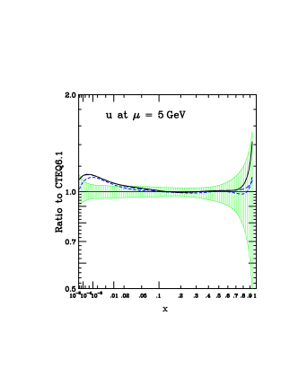
  Figure 17: Ratio of the CTEQ6.5 $u$ density to that of CTEQ6.1, at a scale $Q=5$ GeV. The contour shows the uncertainty at $90\%$ confidence level of the CTEQ6.1 density. From [187].

  A different treatment of heavy flavours in QCD fits can lead to sizable differences. An important update of the CTEQ6.5 fit compared to the previous release, CTEQ6.1, came from the treatment of heavy quarks in a general mass variable flavour number scheme. Using this scheme instead of the ZM-VFNS scheme lead to a considerable improvement of the fit, the $\chi^{2}$ of the fit being reduced by $\sim 200$ units for $\sim 2700$ data points. The resulting CTEQ6.5 PDFs mainly differ from the previous CTEQ6.1 fit by larger $u$ and $d$ distributions in the region $x\sim 10^{-3}$, for a wide range in $Q^{2}$, as illustrated in Fig. 17. This resulted in a $\sim 8\%$ increase of the predicted $W$ and $Z$ cross sections at the LHC, compared to previous CTEQ estimates, and brought the CTEQ-based prediction closer to that obtained using the MSTW08 parton distributions. The uncertainties associated to the remaining freedom in defining a GM-VFNS at NLO or NNLO have been studied in [193]. At NLO, they result in a $2-3\%$ uncertainty on the $Z$ production cross section at the LHC.

• The values of the heavy quark masses $m_{c}$ and $m_{b}$ differ between analyses, and in some cases are treated as free parameters of the fit. The values chosen also depend on the renormalisation scheme used to define them and to calculate heavy quark related observables. The on-shell scheme uses the pole mass, defined to coincide with the pole of the heavy quark propagator at each order of pQCD. This definition is chosen in most QCD analyses. Instead, the $\overline{MS}$ scheme, used in the recent ABM11 analysis [81], introduces a running mass $m_{q}(Q^{2})$. It was shown in [194] that the perturbative stability of predictions for the heavy quark structure functions is better in terms of the $\overline{MS}$ mass, thus leading to reduced theoretical uncertainties due to variations of the renormalisation and factorisation scales. In most QCD analyses, the masses $m_{c}$ and $m_{b}$ are fixed in the fit, and fits obtained when the masses are varied from the chosen central values may be provided together with the central fit. In the ABM11 analysis, $m_{b}(Q=m_{b})$ and $m_{c}(Q=m_{c})$ are fitted together with the PDF parameters, with external constraints given by their world average values. The HERA experiments have also performed preliminary fits where the PDFs are fitted together with the pole mass of the charm quark [114].

• The value of the strong coupling constant $\alpha_{s}(M_{Z})$ is an important consideration in any QCD analysis, unless it is treated as a free parameter in the fit. Many experimental observables can be used to measure $\alpha_{s}(M_{Z})$. The world averages of $\alpha_{s}(M_{Z})$ do not include the measurements of scaling violations of the structure function $F_{2}$, as $\partial F_{2}/\partial\ln(Q^{2})$ is sensitive to the product of $\alpha_{s}$ times the gluon density. However, $\alpha_{s}(M_{Z})$ can be determined together with the parton distribution functions in a combined QCD analysis. In order to disentangle the gluon density from the strong coupling constant, these QCD fits should include jet data in addition to structure function measurements [195, 196]. In the central fit of the MSTW08 and ABM11 analyses, $\alpha_{s}(M_{Z})$ is fitted together with the other parameters that define the PDFs at the starting scale. In contrast, other groups fix $\alpha_{s}(M_{Z})$ and provide several sets of fits, corresponding to a range of fixed $\alpha_{s}$ values.

• Different numerical methods can be used to calculate the theoretical cross sections that are needed in the fit. Indeed, while the NLO calculation of inclusive DIS cross sections can be done relatively fast, the exact calculation of jet cross sections, for example, using standard techniques requires huge CPU resources and, in practice, numerical approximations have to be used when such processes are included in a NLO QCD fit (where the calculation of cross sections has to be done for every iteration of the fit). For example, the FastNLO technique [197] allows rapid calculations for a large number of jet cross sections, with a very high accuracy. The method rewrites the cross sections as a sum of products where the time-consuming step is factorised out, such that it needs to be done only once. This approach is used by the MSTW and NNPDF groups to calculate the jet cross sections. A similar technique is used in APPLgrid [198] which covers a broader range of processes and in the FastKernel approach [176] developed by the NNPDF collaboration. Alternatively, or for processes for which no fast NLO calculation is available, a “K-factor” approximation can be used. For each bin of the experimental measurement, the factor $K=\sigma_{NLO}/\sigma_{LO}$ is first calculated for a given PDF. In the calculations performed in each iteration of the fit, only the leading order cross section is calculated, and it is multiplied by this factor $K$ to account for the higher order corrections. Usually the procedure is repeated in which the $K$-factor is re-evaluated using the PDFs from the converged fit and another series of fit iterations is performed.

Moreover, the fits usually require basic consistency constraints to be satisfied. For example, a set of parameters that would lead to negative cross sections, negative values of $F_{2}$ or of $F_{L}$, should not be considered as a valid fit. On the other hand, a valid fit may result, for example, in a negative gluon distribution at low $x$, since a parton distribution function is not a physical observable.

3.2.3 Parameterisation choices and assumptions

In any QCD analysis, a priori choices have to be made to define the starting conditions. These are: the starting scale of the fit, the set of densities that are parameterised, and the functional form chosen for the parameterisation. Some assumptions usually complement these choices. The systematic uncertainty that should be associated with these choices is not easy to assess and is usually not estimated explicitly.

Large values of the starting scale $Q^{2}_{0}$ are unpractical. Indeed, since DGLAP evolution has the effect of washing out the $x$-dependence of PDFs with increasing $Q^{2}$, parameterising the densities at a low scale offers more freedom in the fit. However, the scale $Q^{2}_{0}$ cannot be too low, since the DGLAP evolution should be valid down to that scale. Typical values for $Q^{2}_{0}$ range between $1$ GeV² and a few GeV². For fits that treat the heavy flavours in a GM-VFNS scheme, it is convenient to set the scale $Q^{2}_{0}$ below the charm threshold, $Q^{2}_{0}<m^{2}_{c}$, such that $c(x,Q^{2}_{0})=0$. The GJR group uses a lower starting scale, for example $Q^{2}_{0}=0.5$ GeV² in [178]. They assume that all PDFs have a valence form (i.e. the parameter $\alpha$ in Eq. 43 is positive) at a low scale; the gluon and sea quarks tend to zero at low $x$, and the large values for these PDFs at $Q^{2}$ above a few GeV² are entirely generated by the DGLAP evolution.

The set of parton densities that are parameterised at the starting scale of the fit, and that are the input to the evolution equations, has to be chosen depending on the experimental measurements that are included in the fit. One does not fit the eleven quark and gluon distributions since the data do not contain enough information to disentangle them all. Instead, well-defined combinations of PDFs are fitted. In addition to the gluon density, at least two quark distributions are needed (one singlet distribution that evolves as Eq. 22, one non-singlet that follows Eq. 21). A QCD fit to H1 NC DIS cross sections only, using $xg(x)$ and two quark distributions as input to the DGLAP equations, was performed in [203] and allowed the gluon distribution to be extracted. Additional measurements are necessary in order to also extract the quark densities, and at least four quark distributions need to be parameterised. For example, the HERAPDF1.0 fit [61], described in more detail in 3.4, parameterises $g(x)$, $\bar{U}(x)$, $\bar{D}(x)$ and the valence distributions $u_{v}(x)$ and $d_{v}(x)$, at a starting scale just below the charm threshold. Since the included data have no sensitivity to constrain the strange density, $s(x)$ is assumed to be proportional to $\bar{d}(x)$ at $Q^{2}_{0}$ and $s(x)=\bar{s}(x)$ is assumed. The MSTW08 analysis also parameterises the gluon and valence densities, $g$, $u_{v}$ and $d_{v}$, together with the light sea density $S$ and the $\bar{d}-\bar{u}$ asymmetry. Moreover, since it includes strange-sensitive measurements, the total strangeness density $s+\bar{s}$ and the strange asymmetry $\bar{s}-s$ are also fitted.

The functional form that is used to parameterise these input densities at the starting scale differs depending on the analyses. It should be flexible enough to allow for a good fit. However, too much freedom in the parameterisation should be avoided, as this leads to unstable fits and secondary minima. A functional form like Eq. 43 is often chosen. The low $x$ behaviour is motivated by Regge phenomenology, which suggests (see for example [91]) that $xg(x)$ and $x\bar{q}(x)$ behave at low $x$ as $(1/x)^{\alpha_{P}(0)-1}$ with $\alpha_{P}(0)\sim 1.08$, while the valence distributions depend instead on the “Reggeon intercept” $\alpha_{R}(0)\sim 0.5$, i.e. $xq_{v}(x)\sim(1/x)^{\alpha_{R}(0)-1}\sim x^{0.5}$. The high $x$ behaviour can be motivated by simple dimensional arguments [204] based on the energy dependence of the scattering cross section. While these predictions were approximately borne out by early measurements, the existing experimental data now show that the PDFs can not be described by a single power-law at high $x$, hence the correction function $P_{i}(x)$ in Eq. 43 is necessary.

The HERAPDF or MSTW analyses take $P_{i}(x)$ to be of the form

$$P_{i}(x)=1+a_{i}x+b_{i}\sqrt{x}+...\qquad,$$

whereas in the fits performed by the CTEQ/CT collaboration, it is chosen as

$$P_{i}(x)=\exp(a_{i}x+b_{i}\sqrt{x}+c_{i}x+d_{i}x^{2})\qquad.$$

In recent global fits, additional flexibility is needed for the gluon distribution, in order to obtain a good fit to all the data. The MSTW08 analysis uses

$$xg(x)=A_{g}x^{\alpha_{g}}(1-x)^{\beta_{g}}(1+a_{g}x+b_{g}\sqrt{x})+A^{\prime}_{g}x^{\alpha^{\prime}_{g}}(1-x)^{\beta^{\prime}_{g}}$$ (46)

which allows the gluon density to become negative at low $x$, while, in the CT10 analysis, extra freedom at low $x$ is given by

$$xg(x)=A_{g}x^{\alpha_{g}}(1-x)^{\beta_{g}}\exp(a_{g}x+d_{g}x^{2}-e_{g}/x^{k_{g}})\qquad.$$ (47)

The number of free parameters is usually reduced by imposing the number sum rules, Eq. 3 and Eq. 4, together with the momentum sum rule, Eq. 20, which helps fix the gluon normalisation and connects the low $x$ and high $x$ behaviour of the gluon density. Additional assumptions are often made. For example, the CT10 analysis assumes the same low $x$ power-law for the input distribution $x\bar{u}$ and $x\bar{d}$, i.e. $\alpha_{\bar{u}}=\alpha_{\bar{d}}$ in Eq. 43, as well as the equality of the normalisation parameters, $A_{\bar{u}}=A_{\bar{d}}$, such that $\bar{d}-\bar{u}\rightarrow 0$ as $x\rightarrow 0$. A similar assumption is made for the HERAPDF1.0 fit. All in all, there are $10$ free PDF parameters in the HERAPDF1.0 analysis and $26$ free parameters in the CT10 fit. The MSTW08 fit has $29$ free parameters, including the value of $\alpha_{s}(M_{Z})$ which is fitted together with the parton densities.

Although the functional form chosen to parameterise the densities at $Q^{2}_{0}$ is rather flexible, a potential parameterisation bias does remain, that is difficult to avoid. Moreover, the uncertainties, obtained as explained in section 3.3.1, can be considerably underestimated since they usually do not include any parameterisation uncertainty. An example of a parameterisation bias is illustrated in Fig. 18, which shows the relative uncertainty on the gluon density at low $x$, at a scale $Q^{2}=4$ GeV². The huge difference between the uncertainty obtained with CT10 and that resulting from the previous fit CTEQ6.6 is due to the more flexible gluon parameterisation used in the former fit. At low $x$, the CTEQ6.6 parameterisation is equivalent to a single power-law, $xg(x)\sim Ax^{\alpha}$. Neglecting the correlation between the $A$ and $\alpha$ parameters, this parameterisation prevents the relative uncertainty from growing faster than linearly with respect to $\ln x$, since $\Delta(xg)/g=(\Delta\alpha)\ln x$. As there is no experimental data at $x$ below $10^{-5}$ and $Q^{2}$ above the typical lower $Q^{2}$ cut used in the fits, the small uncertainty band resulting from the CTEQ6.6 fit can only be artificial. Indeed, using a very similar experimental input, but the more flexible parameterisation Eq. 47 for the gluon density, the uncertainty increases dramatically as shown by the CT10 contour in Fig. 18. With this more flexible parameterisation, the CT uncertainty becomes comparable to that obtained by MSTW08, where extra freedom to the low $x$ gluon is provided by Eq. 46.

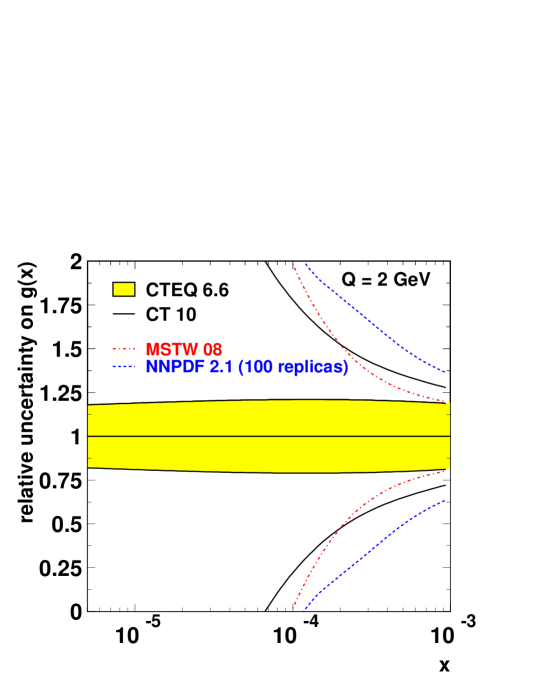
Figure 18: Relative uncertainty ($90\%$ confidence level contours) on the gluon density at $Q^{2}=4$ GeV², as obtained from the CTEQ6.6, CT10, MSTW08 and NNPDF2.1 analyses.

The parameterisation bias can be assessed, to some extent, by varying the starting scale $Q^{2}_{0}$, and / or by making variations around the chosen functional form at the given $Q^{2}_{0}$ and providing an additional parameterisation uncertainty, as pioneered in [60] and also estimated in the HERAPDF analysis; however, the resulting uncertainties remain subjective.

Alternative choices for the densities $xf_{i}(x)$ can be based on Chebyshev polynomials, on any interpolation polynomials, or on non-linear functions. The latter approach is exploited by the NNPDF collaboration, which uses neural networks to parameterise the densities. The formalism is described in [176] and references therein. Neural networks are just another functional form, that generalises parameterisations like $xf(x)=\sum_{n}\alpha_{n}P_{n}(x)$ based on interpolation polynomials $P_{n}(x)$. They allow non-linear dependencies of the function on the fitted parameters $\alpha_{n}$.

The analysis presented in [176] fits the gluon density together with the six densities for light quarks and anti-quarks, $u,\bar{u},d,\bar{d},s,\bar{s}$. The neural networks chosen to parameterise these densities have $37$ free parameters each. Hence, the resulting parameterisation has a total of $7\times 37=259$ free parameters, which is much larger than the number of free parameters, ${\cal{O}}(25)$, which are fitted in QCD analyses based on a standard functional form like Eq. 43. The use of such a flexible parameterisation scheme considerably reduces any parameterisation bias.

3.3 Treatment of experimental systematic uncertainties

3.3.1 The various methods

A lot of work has been done over the past $\sim 15$ years to assess the uncertainties on parton densities extracted from QCD fits [183]. The task is not trivial since, as soon as many experimental data points are included in the fit, a standard statistical approach does not appear to be adequate, as will be discussed in 3.3.2.

While most of the fits now minimise a $\chi^{2}$ function similar to Eq. 44 and Eq. 45, this $\chi^{2}$ definition can be used in different ways:

• in the so-called “offset method” : the parameters $s_{k}$ are set to zero in the central fit - i.e., the central fit is performed without taking into account the correlated systematic errors. Then, for each source of systematic error, $s_{k}$ is set to $\pm 1$ and the fit is redone. The uncertainty of a given quantity (e.g. a parton density) is calculated by adding in quadrature all differences to the quantity obtained in the central fit.

• in the “Hessian method” : the $s_{k}$ are not fixed, but are parameters of the fit. This means that the central fit is performed to the data shifted by the optimal setting for the systematic error sources as determined by the fit. The errors on the fitted PDF parameters $(p_{\alpha})$ are obtained from $\Delta\chi^{2}=T^{2}$ with $T=1$ or larger, see section 3.3.2. The error on any given quantity $F$ is then obtained from standard error propagation:

  $$\sigma^{2}_{F}=\Delta\chi^{2}\left(\sum_{\alpha,\beta}\frac{\partial F}{\partial p_{\alpha}}C_{\alpha,\beta}\frac{\partial F}{\partial p_{\beta}}\right)$$ (48)

  where the covariance matrix $C=H^{-1}$ is the inverse of the Hessian matrix defined by $H_{\alpha,\beta}=\frac{1}{2}\partial^{2}\chi^{2}/\partial p_{\alpha}\partial p_{\beta}$, evaluated at the $\chi^{2}$ minimum. The method developed in [183], which is now widely used by most groups, allows the Hessian matrix to be diagonalised without numerical instabilities; the error $\sigma_{F}^{2}$ can then be calculated simply as

  $$\sigma^{2}_{F}=\frac{1}{2}\sum_{i}\left(F(S_{i}^{+})-F(S_{i}^{-})\right)^{2}$$ (49)

  where the sum runs over the eigenvectors and $S_{i}^{+}$ and $S_{i}^{-}$ are PDF sets displaced by $\Delta\chi^{2}$ along the $i^{th}$ eigenvector direction. For fits that use the Hessian method to determine the uncertainties, the PDF sets $S_{i}^{+}$ and $S_{i}^{-}$ are stored in the public LHAPDF library, together with the set corresponding to the central fit.

The offset method gives fitted theoretical predictions which are as close as possible to the “raw” data points. It does not use the full statistical power of the fit to correct the data for the best estimate of the systematic shifts, since it distrusts that systematic uncertainties are Gaussian distributed. The offset method thus appears to be more conservative than the Hessian method. It usually results in larger uncertainties than what is obtained from the Hessian method, when the criterion $\Delta\chi^{2}=1$ is used to obtain the error bands. With the Hessian method, model uncertainties (e.g. varying $\alpha_{s}$, $Q^{2}_{0}$, …) are often larger than the fit uncertainties. This is because each model choice can result in different values of the systematic shifts, i.e. when changing the model one does not fit the same data points.

Alternatively, a Monte-Carlo approach can be used (see for example [206]), which avoids the usage of the error matrix formalism of Eq. 48. A set of $N_{rep}$ replicas of the $n$ experimental measurements is built by sampling the probability distribution defined by the data, such that the means, variances and covariances given by the replicas are those of the experimental measurements. The fit is then performed separately on each Monte-Carlo replica. The best fit is defined as the average over the replicas, and uncertainties on physical quantities are obtained as standard variances. This method can be used for any choice of the parameterisation of parton densities, but it is mostly convenient when the parameterisation is more complex than the standard functional form of Eq. 43, leading to a much larger number of free parameters. QCD fits using standard parameterisations like Eq. 43 usually make use of the Hessian matrix method to propagate the systematic uncertainties - that is the case of the analyses performed by the CTEQ and the MSTW groups - although the fit performed by the H1 collaboration in [122] estimated the uncertainties with the Monte-Carlo approach. The NNPDF collaboration, which uses a more flexible parameterisation, always propagates the systematic uncertainties with the Monte-Carlo method. For the NNPDF2.0 analysis presented in [176], an ensemble of $N_{rep}=1000$ replicas of the measurements was used. The result of the $N_{rep}$ fits performed over these replicas (i.e. $N_{rep}$ sets of $259$ parameters each) is stored in the LHAPDF package, and can be used to predict mean values and uncertainties on physical observables.

3.3.2 The tolerance parameter $\boldsymbol{\Delta\chi^{2}=T^{2}}$ in global fits with “Hessian” uncertainties

Ideally, the error bands corresponding to $68\%$ (one standard deviation) confidence level (CL) should be obtained from the well-known criterion $\Delta\chi^{2}=1$, or $\Delta\chi^{2}=2.71$ for the $90\%$ (two standard deviation) contours. This would be appropriate when fitting consistent datasets to a well defined theory, with systematic uncertainties being Gaussian distributed. However, in practice, these conditions are not necessarily fulfilled. For example, when fitting data from various experiments, it can happen that some datasets are marginally compatible with the others, possibly because some systematic uncertainty has been underestimated. Such datasets should not be dropped from the fit unless there is a clear experimental evidence that the measurement is incorrect. Instead, the level of inconsistency between the datasets should be reflected in the uncertainties of the fit. This can be done by considering the sets of PDF parameters as alternative hypotheses, and by allowing all fits for which a desired level of consistency is obtained for all datasets. If a dataset consists of $N$ experimental points, its partial $\chi^{2}$ should be about $N\pm\sqrt{2N}$. Practically, a tolerance parameter $T$ is chosen such that the criterion $\Delta\chi^{2}=T^{2}$ ensures that each dataset is described within the desired confidence level. An example procedure to obtain the numerical value of $T$ can be found in  [207]. For example, the $90\%$ CL contours of CTEQ6.6 correspond to $T=10$ ($T\sim 6$ for $68\%$ CL), while the MRST fits [208] used $T=\sqrt{50}\sim 7$. The MSTW08 analysis uses a “dynamical tolerance” [173] where $T$ can be different for the various eigenvectors of the Hessian matrix, with values ranging between $T\sim 1$ and $T\sim 6.5$ for the $68\%$ CL contours.

While this approach is well motivated and based on how far the parameters can be varied while still giving an acceptable description of all the datasets, one should keep in mind that setting $\Delta\chi^{2}=100$ or $50$ corresponds to an increase of the errors of all experiments by a factor of typically $5-6$, including those for which the measurements are very well controlled.

3.4 QCD fits to DIS data

As seen in section 2.3, the HERA experiments performed high precision measurements of NC and CC DIS in a large kinematic domain, both in $e^{+}p$ and $e^{-}p$ collisions. In particular:

• the precise measurement of the scaling violations of the structure function $F_{2}$ in NC DIS, i.e. its logarithmic dependence on the four-momentum transfer squared $Q^{2}$, gives access to the gluon density at low and medium $x$;

• the precise measurement of $F_{2}$ in NC DIS at low and medium $x$ sets strong constraints on the combination $4(U+\bar{U})+(D+\bar{D})$ where $U$ and $D$ denote the combined up-type and down-type quark densities, $U=u+c$ and $D=d+s+b$;

• the CC DIS measurements provide two constraints: one on a linear combination of $D$ and $\bar{U}$ ($e^{+}p$ data), and one on a linear combination of $U$ and $\bar{D}$ ($e^{-}p$ data);

• the measurement of $xF_{3}$ obtained from the difference of $e^{+}p$ and $e^{-}p$ NC DIS cross sections provides a constraint on a linear combination of $U-\bar{U}$ and $D-\bar{D}$.

As a result, good constraints can be obtained on the gluon density as well as on $U$, $D$, $\bar{U}$ and $\bar{D}$ from HERA data alone. The separation between $U$ and $D$, which in fits to HERA data is provided by the CC measurements, can be further improved by including e.g. DIS measurements on a deuterium target. In fits based only on inclusive DIS measurements, separating further $U$, $D$, $\bar{U}$ and $\bar{D}$ along the individual quark flavours mostly relies on assumptions.

3.4.1 Fit of the combined HERA-I inclusive datasets

The HERAPDF1.0 parton densities [61] were extracted using only the averaged H1 and ZEUS DIS measurements presented in section 2.3.4. The averaged HERA dataset corresponds to $741$ cross section measurements: $528$ ($145$) measurements of $e^{+}p$ ($e^{-}p$) NC DIS and $34$ measurements of both $e^{+}p$ and $e^{-}p$ CC DIS. Following a cut $Q^{2}>Q^{2}_{min}$ with $Q^{2}_{min}=3.5$ GeV², imposed to remain in the kinematic domain where pQCD is reliable, $592$ data points are included in the QCD fit of [61]. The fit is performed at NLO within the general mass variable flavour number scheme of [190, 191]. The starting scale is chosen to be slightly below the charm threshold, $Q^{2}_{0}=1.9$ GeV².

The initial parton distributions $xf=xg,xu_{v},xd_{v},x\bar{U}$ and $x\bar{D}$ are parameterised at $Q^{2}_{0}$ using the generic form:

$$xf(x)=Ax^{B}(1-x)^{C}(1+\epsilon\sqrt{x}+Dx+Ex^{2})$$ (50)

At low $x$ the assumptions $\bar{d}/\bar{u}\rightarrow 1$ as $x\rightarrow 0$ and $B_{u_{v}}=B_{d_{v}}$ are made, which together with the number and momentum sum rules, removes $6$ free parameters of the fit. The strange quark distribution, $x\bar{s}=f_{s}x\bar{D}$, is expressed as a $x-$independent fraction, $f_{s}=0.31$, of the down-type sea at the starting scale.

A $9$-parameter fit is first performed by setting to zero all $\epsilon$, $D$ and $E$ parameters in Eq. 50. These parameters are then introduced one by one, the best $10$-parameter fit having $E_{u_{v}}\neq 0$. As a result, the central fit of HERAPDF1.0 is a $10$-parameter fit corresponding to the following parameterisation:

$$xg(x) = A_{g}x^{B_{g}}(1-x)^{C_{g}}$$ (51)

$$xu_{v}(x) = A_{u_{v}}x^{B_{u_{v}}}(1-x)^{C_{u_{v}}}\left[1+E_{u_{v}}x^{2}\right],$$ (52)

$$xd_{v}(x) = A_{d_{v}}x^{B_{d_{v}}}(1-x)^{C_{d_{v}}},$$ (53)

$$x\bar{U}(x) = A_{\bar{U}}x^{B_{\bar{U}}}(1-x)^{C_{\bar{U}}},$$ (54)

$$x\bar{D}(x) = A_{\bar{D}}x^{B_{\bar{D}}}(1-x)^{C_{\bar{D}}}.$$ (55)

The fit has a $\chi^{2}$ of $574$ for $582$ degrees of freedom. Example PDFs at the scale $Q^{2}=10$ GeV² are shown in Fig. 19, together with their uncertainties obtained as described below.

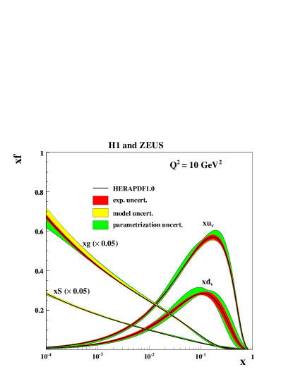
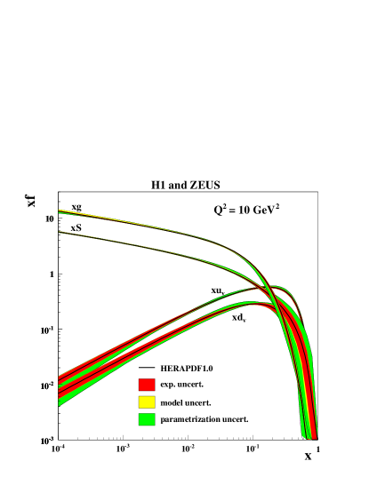
Figure 19: Distributions of valence quarks densities $xu_{v}$ and $xd_{v}$, of the gluon density $xg$ and of the density of sea quarks $xS$ obtained from the fit to the HERA-I dataset, at $Q^{2}=10$ GeV², together with one standard deviation uncertainties. From [61].

The experimental uncertainty of the HERAPDF1.0 PDFs (shown as the red band in Fig. 19) is determined using the Hessian method described in section 3.3.1, taking into account the $110$ sources of systematic errors of the individual measurements together with their correlations. The tolerance criterion $\Delta\chi^{2}=1$ is used to determine the $1\sigma$ error bands. Three additional errors are included which account for different treatment of the systematic uncertainties in the averaging procedure of the H1 and ZEUS measurements. These are the largest uncertainties and are included using the more conservative offset method. Very good constraints are obtained on $U$, $D$, $\bar{U}$ and $\bar{D}$, which are the combinations the measurements are directly sensitive to, in a large range of $x$ extending down to $10^{-4}$ and up to ${\cal{O}}(0.1)$. As expected, the best constraints are obtained on $U$, with an uncertainty that remains below $10\%$ for $x\,\lower 1.07639pt\hbox{$\scriptstyle\sim$}\kern-5.59721pt\raise 2.36806pt\hbox{$\scriptstyle<$}\,0.5$. The gluon PDF is also well constrained up to $x\sim 0.2$, and down to $x\sim 10^{-4}$.

The model uncertainty, shown as the yellow band in Fig. 19, is obtained by varying the input values of $f_{s}$, $m_{c}$, $m_{b}$ and $Q^{2}_{min}$ and repeating the fit. The largest effect comes from the variation of $f_{s}$ and of the heavy quark masses, which affects considerably the strange and charm densities.

Following [60], an assessment of the additional uncertainty that is introduced by the parameterisation choice is made in this analysis. This is particularly relevant since the number of parameters in the central parameterisation of this analysis (Eq. 52-55) is rather small ($10$). The variation of the starting scale $Q^{2}_{0}$ is included in this parameterisation uncertainty. Indeed, when the DGLAP equations are used to perform a backward evolution of the gluon distribution obtained from the central fit, from $Q^{2}_{0}=1.9$ GeV² down to $1.5$ GeV², the resulting function cannot be fitted by the simple form of Eq. 51. Consequently, repeating the fit with a lower starting scale $Q^{2}_{0}=1.5$ GeV² results in large differences compared to the central fit if the same parameterisation is kept, because Eq. 51 is not flexible enough to describe the gluon distribution at low scales. Hence, when the fit is repeated with $Q^{2}_{0}=1.5$ GeV², additional freedom is given for the gluon distribution by subtracting a term $A^{\prime}_{g}x^{B^{\prime}_{g}}(1-x)^{C^{\prime}_{g}}$ to Eq. 51, as first suggested in [173], where $C^{\prime}_{g}$ is fixed to a large value which ensures that this additional term does not contribute at high $x$. Moreover, an additional fit is performed using the parameterisation of the central fit but relaxing the assumption $B_{u_{v}}=B_{d_{v}}$. Alternative $11$-parameter fits with $E_{u_{v}}\neq 0$ are also considered, including those which lead to good fit quality but peculiar behaviour at large $x$. An envelope is constructed, representing the maximal deviation, at each $x$ value, between the central fit and the fits obtained using these parameterisation variations. This envelope defines the parameterisation uncertainty of HERAPDF1.0 and is shown separately in Fig. 19 as the green band. The gluon and sea PDFs at low $x$ are mostly affected by the variation of $Q^{2}_{0}$ while at large $x$ (and over the whole $x$ range for the valence distributions), adding an eleventh parameter in the fit dominates the parameterisation uncertainty. The total PDF uncertainty is obtained by adding in quadrature the experimental, model and parameterisation uncertainties. In particular, the parameterisation uncertainty increases considerably the uncertainty of the gluon PDF at $x\sim 0.1$ and beyond.

3.4.2 Impact of jet data on the fits to HERA data

As seen in Fig.19, the precision on the gluon density is limited at medium and high $x$ when only inclusive HERA data are used. Adding HERA data from jet production in DIS and in photoproduction was shown to lead to better constraints [209]. Although HERA jet data do not bring strong constraints on the gluon density at high $x$ due to the limited statistics (better constraints at high $x$ are brought by Tevatron jet data), they can be useful for medium $x$, since HERA jet cross sections have small systematic uncertainties (typically $5\%$, a factor of at least $2$ smaller than the systematic uncertainties of jet cross sections measured by the Tevatron experiments, see section 2.4.3). For the fits performed using only HERA DIS inclusive data [209], the uncertainty of the gluon density was reduced by a factor of $\sim 2$ in the mid-$x$ region, $x=0.01-0.4$, when measurements of inclusive jet production at HERA (see Fig. 10) were included. It is also interesting to note that both fits, with and without the jet data, lead to the same shape for the gluon density, indicating that there is no tension between the HERA jet and inclusive DIS data. Similar conclusions were reached in preliminary fits using the full statistics of HERA data [114].

3.4.3 Fits performed using preliminary combinations of HERA data

Following HERAPDF1.0, several QCD fits have been performed to preliminary combinations of HERA data. As for HERAPDF1.0, the extraction of the HERAPDF1.5 PDFs relies on inclusive DIS data only, but a preliminary combination of H1 and ZEUS measurements from HERA-I and HERA-II was used instead of the published HERA-I combined dataset. This fit was also performed with additional freedom given to the gluon and the $u_{v}$ parameterisation in Eq. 51 and 52, leading to $14$ free parameters instead of $10$ (HERAPDF1.5f). This extended parameterisation was also used for the extraction of NNLO PDFs, HERAPDF1.5 NNLO. These fits, although unpublished, are available in the LHAPDF interface. H1 and ZEUS jet data were added in order to extract the HERAPDF1.6 (NLO) PDFs. The most recent preliminary fit, HERAPDF1.7, also includes the $F_{2}^{c\bar{c}}$ measurements and the data taken in $2007$ with a lower proton beam energy. Further details can be found in [114, 210].

3.4.4 Impact of fixed target DIS data

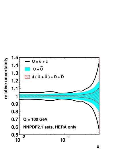
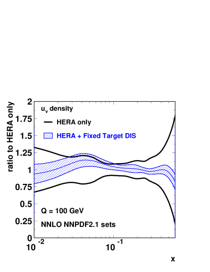
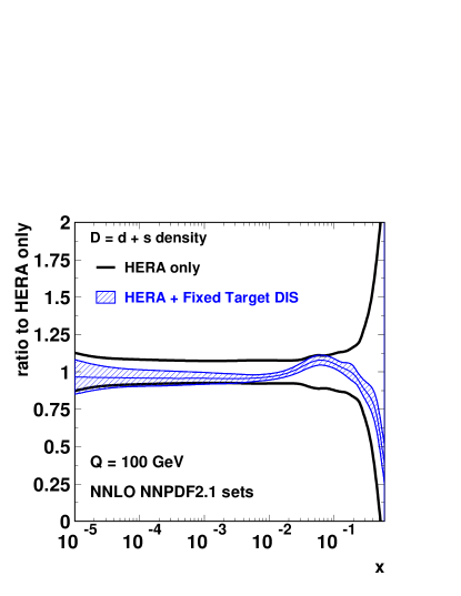
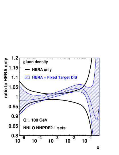
Figure 20: Top left: relative uncertainties on example quark densities obtained from the NNPDF fit to HERA data alone. Top right and bottom: comparison of the results of the fits with and without the fixed target data for the $u_{v}$, $D$ and gluon distributions. The contours correspond to one standard deviation uncertainties.

In fits based on HERA data alone, the flavour separation, as well as the separation between quarks and anti-quarks (i.e. between valence and sea quarks) is provided by the high $Q^{2}$ measurements of CC cross sections and of $xF_{3}$ in NC interactions. This separation, in particular at high $x$, can be further improved by adding measurements of fixed target DIS experiments to the fitted data. In particular, the $F_{2}^{d}$ measurements of BCDMS and NMC mostly set a constraint on $4d+u$ which nicely complements that on $4(U+\bar{U})+(D+\bar{D})$ set by lepton-proton measurements of $F_{2}^{p}$. Moreover, the measurements made in neutrino DIS provide direct access to the distribution of valence quarks, assuming that nuclear corrections are under control.

In [211], the improved determination of quark distributions brought by the addition of fixed target measurements in a fit to HERA data was studied within the fitting framework of the ZEUS experiment. Here, the complementarity between HERA data and fixed target DIS measurements is illustrated by using the series of fits performed by the NNPDF collaboration, identical to the NNPDF2.1 analysis but using subsets of experimental data. These fits are described in [177] and have been released in the LHAPDF package. In particular, a fit has been performed using only the HERA data (the combined HERA-I NC and CC datasets from H1 and ZEUS, inclusive $e^{-}p$ HERA-II measurements from ZEUS [121, 125], as well as $F_{L}$ and $F_{2}^{c\bar{c}}$ measurements). With respect to HERAPDF1.0 the fitting method used here largely avoids any parameterisation bias. A similar fit has been performed by also including data from the fixed target DIS experiments described in section 2.2.

Figure 20 (top left) shows relative uncertainties on example quark densities resulting from the fit to HERA data only. While the combination $4(U+\bar{U})+(D+\bar{D})$ that is directly probed by the $F_{2}^{p}$ measurements is well constrained over the full $x$ range, the uncertainty increases at high $x$ when one tries to separate up-like from down-like distributions, and quarks from anti-quarks. The much improved separation of valence and sea densities provided by the fixed target DIS data is illustrated in Fig. 20 (top right) with the example of the $u_{v}$ distribution. The distributions of down-like quarks obtained from the two fits are compared in Fig. 20 (bottom left). Again a much better determination at medium and high $x$ is achieved when the fixed target data are included in the fit, resulting in a reduced high $x$ distribution. In contrast, the constraints at low $x$ are largely coming from HERA data. Figure 20 (bottom right) shows that the gluon determination is not improved significantly by the addition of fixed target data in the fit.

The next section will show how the determination of quark densities at high $x$, in particular the separation between quarks and anti-quarks, can be further improved by including Drell-Yan measurements in the fits (section 3.5.3). It should also be noted that this determination will benefit from the stronger constraints brought by the full $e^{-}p$ and $e^{+}p$ HERA-II measurements at high $Q^{2}$, which show a much better precision than the HERA-I measurements for example on $xF_{3}$, and from the final HERA combination. The specific impact of the $e^{-}p$ and $e^{+}p$ HERA-II data from H1 was studied in [122] within an analysis framework similar to that used for HERAPDF1.0 and found indeed to be significant.

3.5 Global QCD fits

Although HERA data alone can determine the distributions of all partons, albeit with a limited precision at high $x$, the determination of parton densities in the proton is considerably improved by including additional datasets. The following datasets are routinely included in “global” pQCD analyses of the proton structure.

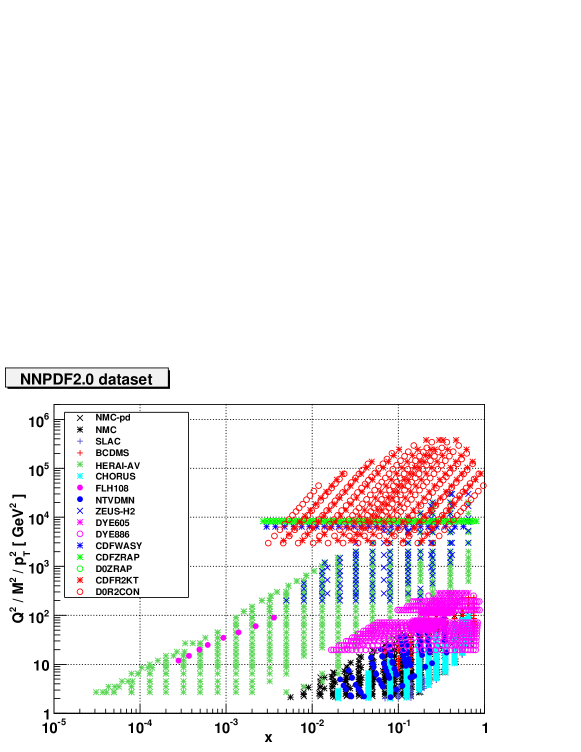
Figure 21: Experimental data which enter in the NNPDF global analysis (from [176]).

As shown in section 3.4.4, the inclusive NC DIS measurements from fixed target experiments using a deuterium target and the CC DIS measurements from the $\nu N$ experiments improve the flavour separation and allow better disentanglement between the quarks and the anti-quarks (i.e. the sea and the valence distributions). The Drell-Yan measurements $pN\rightarrow\mu\mu$ mostly constrain the sea densities. In particular, they set important constraints on the anti-quark densities at medium and high $x$, which are not well known from DIS data alone. Comparing the Drell-Yan cross sections measured in $pp$ and $pd$ provides important constraints on the ratio $\bar{d}/\bar{u}$ at medium $x$.

The exclusive production of muon pairs in neutrino-nucleon scattering, $\nu_{\mu}s\rightarrow\mu c\rightarrow\mu\mu X$, is the only pre-LHC process that sets direct constraints on the strange density.

The Tevatron measurements of inclusive jet cross sections set the strongest constraints on the gluon density at high $x$. The measurements of $W$ and $Z$ production at the Tevatron mostly constrain the $u$ and $d$ densities in the valence domain. Since the $u$ density is already well constrained by the DIS experiments, they improve our knowledge of the $d$ density and of the ratio $d/u$ at medium $x$.

The addition of non-HERA data in the QCD analyses typically leads to ${\cal{O}}(3000)$ data points to be included in the fit. Fig. 21 shows how the experimental data included in the NNPDF2.0 and NNPDF2.1 analyses are distributed in the $(x,Q^{2})$ plane. These two fits include $2841$ points from DIS experiments (with $743$ HERA points), $318$ points of Drell-Yan production in fixed target experiments, $186$ points of jet production at the Tevatron, and $70$ points of vector boson production by D0 and CDF.

In this section we mostly discuss results from the MSTW08, CT10 and NNPDF2.1 NLO analyses. They are based on a similar experimental input and use a GM-VFNS for the treatment of heavy flavours. The MSTW08 analysis parameterises $g$, the valence quark densities $u_{v}$ and $d_{v}$, the light sea $S=2(\bar{u}+\bar{d})+s+\bar{s}$, the asymmetry $\Delta=\bar{d}-\bar{u}$, the total strangeness $s^{+}=s+\bar{s}$ and the strange asymmetry $s^{-}=s-\bar{s}$ at a starting scale $Q^{2}_{0}=1$ GeV². The CT10 analysis parameterises $g$, $u_{v}$, $d_{v}$, $\bar{u}$, $\bar{d}$, $s$ at $Q^{2}_{0}=1.69$ GeV² and assumes $s=\bar{s}$. The NNPDF2.1 analysis parameterises the gluon density and the six quark and anti-quark light flavours at a scale $Q^{2}_{0}=2$ GeV². In the MSTW08 analysis, $\alpha_{s}(M_{Z})$ is fitted together with the PDF parameters, while in the CT10 and NNPDF2.1 fits it is set to a constant value.

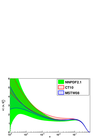
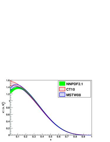
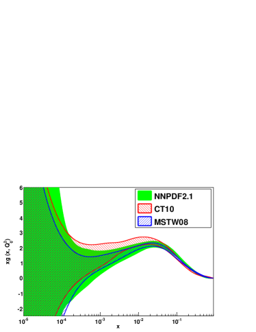
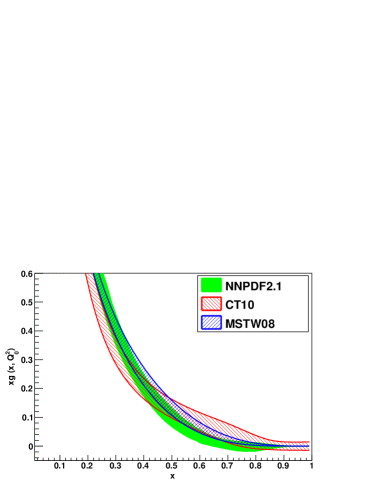
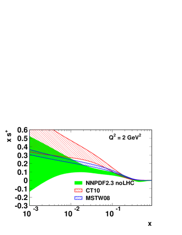
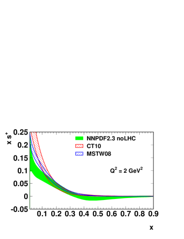
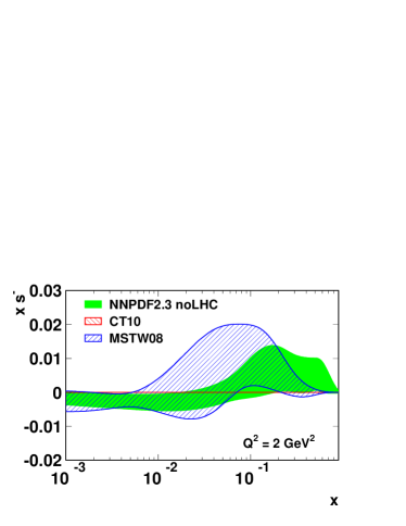
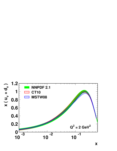
Figure 22: Comparison of recent global fits at $Q^{2}=2$ GeV², for the singlet density $\sum=\sum(q+\bar{q})$, the gluon density (from [177]), the total strangeness $s^{+}=s+\bar{s}$, the strange asymmetry $s^{-}=s-\bar{s}$ and the total valence distribution. Contours at $68\%$ confidence level are shown.

Figure 22 compares a few example PDFs at $Q^{2}=2$ GeV², as extracted from MSTW08, CT10 and NNPDF2.1 The agreement for the gluon density at low and medium $x$ is rather good. In particular, the error band of CT10 is much larger than the one previously predicted from CTEQ6.6, which used a less flexible parameterisation for the gluon density (see Fig. 18), and agrees with that obtained with MSTW08 and NNPDF2.1. At high $x$ however, the gluon densities predicted by the three fits show sizable differences. Moreover, the three fits lead to very different predictions for the strange densities $s^{+}$ and $s^{-}$, although they all use the same strange-sensitive datasets. The NNPDF fit makes no assumption on the shape of the total strangeness density $s^{+}=s+\bar{s}$, in contrast to the MSTW08 and CT10 fits (see section 3.5.5). This results in a larger error band, which impacts the uncertainty of other flavour PDFs at low $x$, especially that of the down quark, since the main constraint on low $x$ quarks comes from the HERA measurement of $F_{2}$, which probes charge weighted sums of quark PDFs. Some differences can also be seen in the valence distribution, in particular for $x\sim 0.1$. Since the error band of the NNPDF2.1 fit is not much larger than that of the other fits, it is unlikely that this difference comes solely from a parameterisation bias; it could be due to, for example, differences in the treatment of nuclear corrections to neutrino DIS data, which set important constraints on the valence densities [38]. The next paragraphs show a more detailed comparison of these three fits, together with the specific impact of the non-DIS datasets.

3.5.1 Tevatron data on $\boldsymbol{W}$ and $\boldsymbol{Z}$ production and the $\boldsymbol{d/u}$ ratio

As shown in section 2.4.3, the shape of the rapidity distribution of $W$ and $Z$ bosons at the Tevatron provides interesting constraints on the $u$ and $d$ densities at $x\,\lower 1.07639pt\hbox{$\scriptstyle\sim$}\kern-5.59721pt\raise 2.36806pt\hbox{$\scriptstyle>$}\,0.01$. The $W$ charge asymmetry constrains the ratio $d/u$ and its slope. This ratio is otherwise mostly constrained by the ratio $F_{2}^{p}/F_{2}^{d}$ measured by the NMC experiment, and by the deuterium measurements of BCDMS. In practice, the Tevatron constraints on $d/u$ are mostly constraints on the down density, since the density of up quarks is much better known in that range.

CDF Run I data on the $W$ asymmetry in the electron channel [153] have been included for long in the QCD analyses. They are now complemented by more precise Run II data [152, 154, 155, 156], some of them [154, 156] being also available in several bins of the lepton transverse energy. Fig. 23 shows the effect of the Run II measurements from CDF [154] and D0 [155], corresponding to a luminosity of $170$ pb^-1 and $300$ pb^-1 respectively, on the extracted down valence distribution. The larger uncertainty obtained in the MSTW08 fit is due to additional freedom introduced in the $d_{v}$ parameterisation, compared to the previous fit MRST2006 [208]. A change in the shape is clearly visible, with a significant increase in $d_{v}$ for $x\sim 0.3$, which is compensated (because of the number sum rule) by a decrease for lower $x$ values.

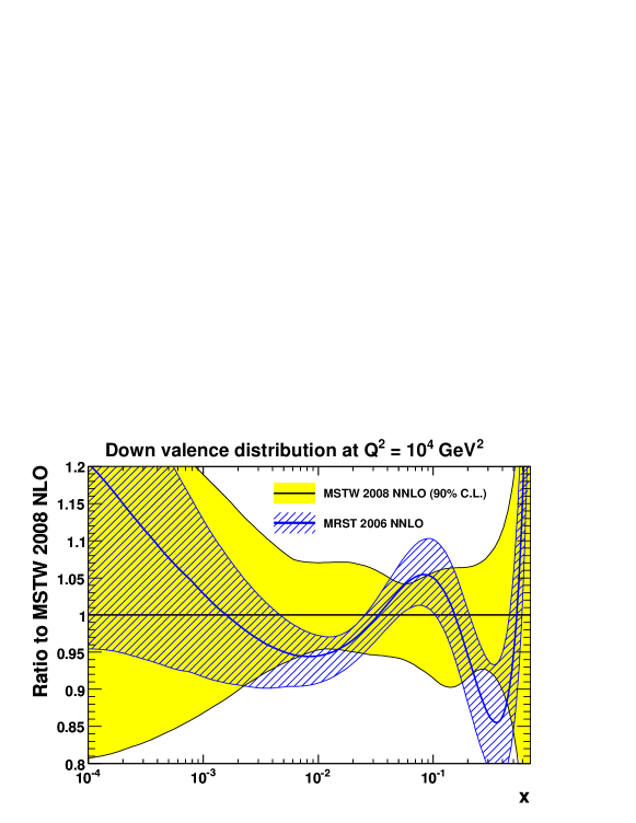
Figure 23: Comparison of $d_{v}$ as extracted from the MSTW analysis, when taking into account the CDF [154] and D0 [155] Run II $W$ asymmetry data (MSTW08), or when using only the CDF Run I measurements (MRST 2006). From [173].

It is interesting to note that the inclusion of the measurements of $W$ charge asymmetry made by D0 in several $E_{T}$ bins using $750$ pb^-1 of Run II data [156] is problematic, as consistently observed by all analyses. These data show some incompatibility with the DIS structure function data, in particular the NMC measurement of $F_{2}^{p}/F_{2}^{d}$ and the BCDMS $F_{2}^{d}$ measurement, and they also show some tension within themselves. The MSTW08 analysis decided not to include the D0 [156] and CDF [152] high luminosity Run II measurements in their fit, pending further investigation. The D0 Run II data of [155, 156] are also excluded from the NNPDF analyses and from the main CT10 fit. However the CTEQ group also provides a fit with these data included (CT10W), obtained by artificially increasing the weight of these datasets in the global fit. Figure 24 compares the $d/u$ ratios obtained from these two fits. The ratio obtained from the CT10W fit has a markedly different slope at $x>0.01$, and a much reduced uncertainty as compared to CT10. While the outcome of the CT10W fit has to be used with care until the compatibility with other data is better understood, this shows the potentially large implications that precise $W$ asymmetry data from the Tevatron can have on the $d/u$ ratio, and hence on the down density at large $x$.

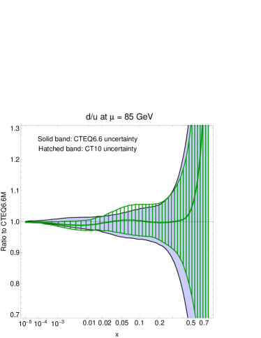
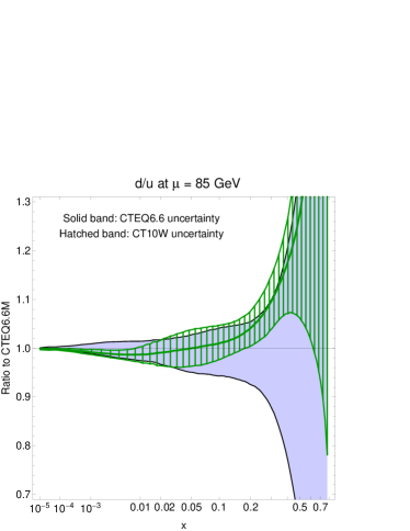
Figure 24: The $d/u$ ratio obtained from the latest CT10 fit without including the Run II D0 measurements on the $W$ charge asymmetry (left), and with these measurements included (right). The ratio is normalised to that derived from the previous CTEQ fit (CTEQ6.6). The uncertainty bands correspond to two standard deviations. From [175].

3.5.2 The asymmetry of the light sea

The combination of constraints from muon-proton and muon-deuteron DIS, from HERA data, and from neutrino DIS data, is not enough to determine the light sea asymmetry $\bar{d}-\bar{u}$, which is very loosely constrained by a fit which includes DIS data only. The inclusion of Drell-Yan data (mostly proton and deuteron fixed target data) dramatically improves this determination, as shown in Fig. 25. Including Tevatron data in addition does not further reduce the uncertainty in a significant manner. The figure was obtained from a series of fits performed by the NNPDF collaboration, identical to the NNPDF2.1 analysis but using subsets of experimental data, which have been released in the LHAPDF package.

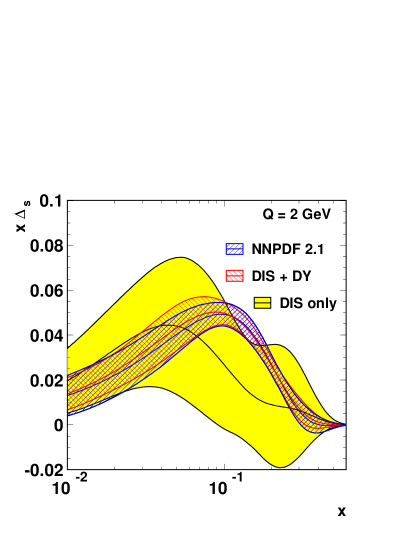
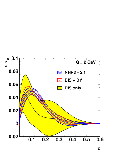
Figure 25: The asymmetry of the light sea $\Delta_{s}(x)=\bar{d}(x)-\bar{u}(x)$ and its one standard deviation uncertainty at $Q=2$ GeV as obtained from the NNPDF analysis, when only DIS data are included in the fit (yellow contour), when Drell-Yan data are included in addition (red hashed contour), and from the reference NNPDF2.1 fit (blue hashed contour).

3.5.3 Quarks and anti-quarks at high $x$

The Drell-Yan measurements from fixed target experiments are also extremely useful to constrain the quark and anti-quark densities at high $x$. This is illustrated in Fig. 26, which uses again the NNPDF2.1 sets released in the LHAPDF interface. The HERA data alone provide very little constraints on the anti-quark densities at $x\sim{\cal{O}}(0.1)$. Fixed target neutrino DIS experiments, which measured both $\nu N$ and $\bar{\nu}N$ cross sections, provide a separation between the valence and the sea quarks at high $x$. As a result, a fit to the full DIS data reduces the uncertainty on the anti-quark densities at high $x$. However, the resulting uncertainty on $\bar{d}(x)$ remains large, e.g. $\sim 40\%$ at $x\sim 0.2$. With the addition of the fixed target Drell-Yan data, this uncertainty is reduced down to $\sim 10\%$. The other datasets included in NNPDF2.1 do not reduce further the uncertainties.

Figure 26 also shows the uncertainties obtained in a fit using only data from the collider experiments (H1 and ZEUS, D0 and CDF). Although the Tevatron data help constrain the $\bar{d}(x)$ distribution at high $x$, their impact is not as large as that of the Drell-Yan data, and their impact on the uncertainty of $\bar{u}(x)$ at high $x$ is marginal. The measurement of high mass di-lepton production at the LHC will obviously bring further constraints on anti-quarks at high $x$, assuming that effects of physics beyond the Standard Model do not distort the mass spectrum.

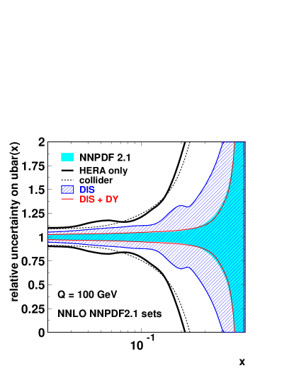
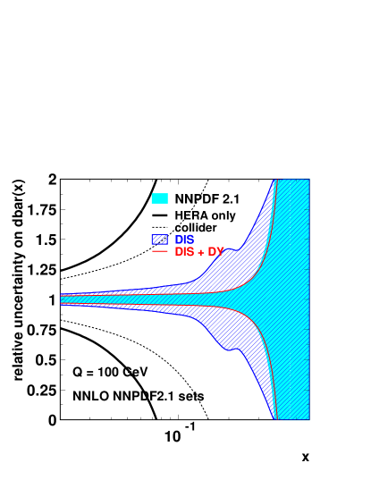
Figure 26: One standard deviation uncertainties on $\bar{u}(x)$ (left) and on $\bar{d}(x)$ (right) at $Q^{2}=10^{4}$ GeV² for $x$ between $0.02$ and $0.6$, as obtained from the NNPDF2.1 global fit (filled area), and from the same fit but applied to a subset of experimental data.

3.5.4 Tevatron jet data and the gluon distribution

The inclusive jet production at the Tevatron experiments is very sensitive to the gluon density at high $x$. Early CDF Run I measurements reported in $1995$ [159] indicated an excess of high $p_{T}$ jets compared to NLO QCD predictions based on the PDFs available at that time. The possibility that this excess could be an indication of quark compositeness created quite some excitement, until it was shown [214] that these jet data could be satisfactorily accommodated in a global fit, which resulted in a larger gluon density at high $x$. While this showed the important role of jet constraints on the gluon density, it also triggered intensive efforts in order to provide PDFs with associated uncertainties, which lead to the state-of-the-art presented above.

The inclusive jet production cross sections measured by D0 and CDF are included in the global QCD analyses since CTEQ4 [214], MRST2001 [215] and NNPDF2.0. Since CT10 and MSTW08, the Run II measurements are used in place of the Run I results. Indeed, these new datasets have a much higher statistics and smaller systematic uncertainties, and the experiments have provided the full correlation matrix of systematic errors. These Run II measurements prefer a smaller high $x$ gluon distribution than the Run I data.

Figure 27 shows the impact of Tevatron jet data on the determination of the gluon density. A fit similar to that of NNPDF2.1 has been performed, using DIS data only, and it is compared to the standard fit of NNPDF2.1. At low $x$, both fits lead to a very similar gluon density, with the same relative uncertainty, meaning that most of the constraints on the gluon density are coming from DIS data (mainly HERA). However, at medium and high $x$, the non-DIS datasets (mainly the jet measurements from the Tevatron experiments) provide a significantly improved uncertainty on the gluon density.

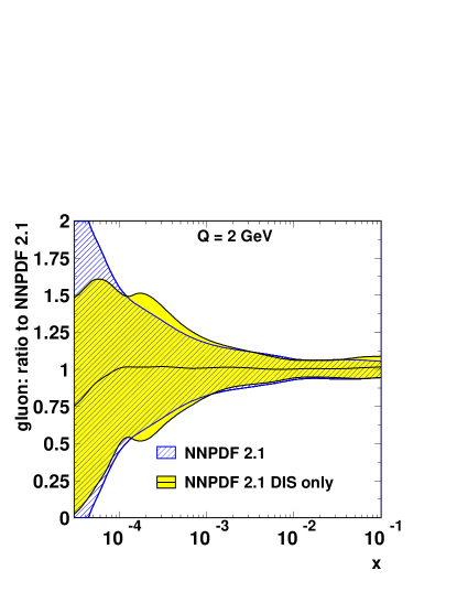
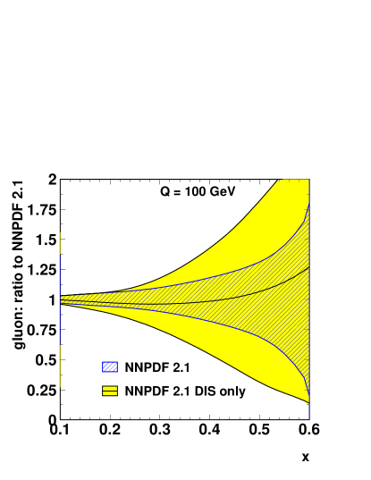
Figure 27: Comparison of the gluon density obtained from NNPDF2.1 and from a similar fit restricted to the DIS data, at low and medium $x$ and $Q=2$ GeV (left), and at high $x$ and $Q=100$ GeV (right). The ratio to the NNPDF2.1 density is shown, together with $68\%$ confidence level contours.

3.5.5 The strange sea

As seen in section 2.2.4, the exclusive production of di-muon events in neutrino DIS experiments, measured by the NuTeV and CCFR experiments, sets constraints on the density of strange quarks for $x\,\lower 1.07639pt\hbox{$\scriptstyle\sim$}\kern-5.59721pt\raise 2.36806pt\hbox{$\scriptstyle>$}\,10^{-2}$ and $x\,\lower 1.07639pt\hbox{$\scriptstyle\sim$}\kern-5.59721pt\raise 2.36806pt\hbox{$\scriptstyle<$}\,0.3-0.4$, via the subprocess $Ws\rightarrow c$. The recent inclusion of these data in global fits allows the strange content of the nucleon to be studied in more details [173, 216]. Previous fits assumed that $s+\bar{s}$ was a constant fraction of the non-strange sea $\bar{u}+\bar{d}$ at the starting scale,

$$s+\bar{s}=\kappa_{s}(\bar{u}+\bar{d})$$

with $\kappa_{s}\sim 0.4-0.5$ reflecting the suppressed probability to produce $s\bar{s}$ pairs compared to $u\bar{u}$ or $d\bar{d}$ pairs. Recent fits however, give more freedom to the strange density in particular at high $x$. This additional freedom leads indeed to an improved $\chi^{2}$.

Both the CTEQ6.6 and the MSTW08 analyses assume that, at low $x$, the strange density follows the same power-law as the light sea density, i.e. $s+\bar{s}\propto x^{\alpha}$ with $\alpha$ set to the low-$x$ power of the light sea (MSTW08) or to that of the $\bar{u}$ and $\bar{d}$ densities (CTEQ6.6). They parameterise the strange density $s+\bar{s}$ as

$$xs+x\bar{s}=Ax^{\alpha}(1-x)^{\beta}P(x)$$

and fit the normalisation $A$ and the high-$x$ power $\beta$. Parameters defining the polynomial function $P(x)$ are also fitted in the CTEQ6.6 analysis, while in MSTW08 they are fixed to be the same as those defining the $g(x)$ of the total sea. The CTEQ6.6 analysis still assumes $s=\bar{s}$, while the MSTW08 analysis parameterises the strange asymmetry as $xs-x\bar{s}=Ax^{\alpha}(1-x)^{\beta}(1-x/x_{0})$ where $x_{0}$ is given by the number sum rule of zero strangeness, and $\alpha$ is fixed to $0.2$ as the data do not constrain $A$ and $\alpha$ independently.

Figure 28 (left) shows the strange density obtained in the two fits, at $Q^{2}=5$ GeV². In the MSTW08 analysis, $s+\bar{s}$ is smaller than $(\bar{u}+\bar{d})/2$, especially at large $x$. The strange density from the CTEQ6.6 fit is considerably larger, even in the range $10^{-2}<x<10^{-1}$ which is directly constrained by the data. The larger uncertainty obtained in the CTEQ6.6 analysis is probably due to the more flexible parameterisation. The uncertainty from the NNPDF2.1 fit, where any parameterisation bias is largely removed, was seen to be even larger (see Fig. 22). Note that the small uncertainty obtained in MRST2001 is due to the assumption $s+\bar{s}=\kappa_{s}(\bar{u}+\bar{d})$ that was made in that fit.

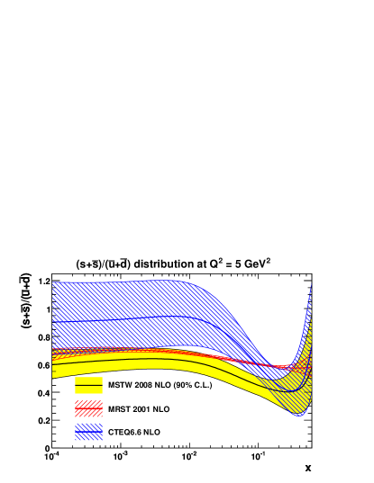
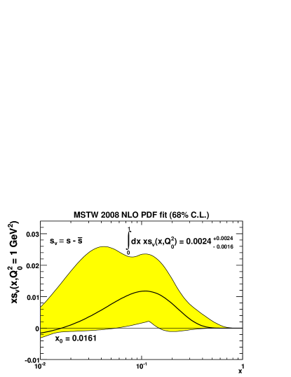
Figure 28: Left: The ratio of the input $s+\bar{s}$ distribution to that of the non-strange sea $\bar{u}+\bar{d}$ at $Q^{2}=5$ GeV², as obtained in the MSTW08, MRST2001 and CTEQ6.6 fits, with $2\sigma$ uncertainty contours. Right: The strange asymmetry $xs-x\bar{s}$ at $Q^{2}_{0}=1$ GeV², together with the $1\sigma$ uncertainty. From [173].

The strange asymmetry $s-\bar{s}$ is actually very loosely constrained, as shown in Fig. 28 (right). The existing data seem to indicate a positive value for the momentum asymmetry $\int dx\,x(s-\bar{s})$ of the strange sea. This asymmetry has important consequences for the $\sin^{2}\theta_{W}$ anomaly reported by the NuTeV collaboration [217]. From the asymmetry between $\sigma(\nu_{\mu}N\rightarrow\nu_{\mu}X)$ and $\sigma(\bar{\nu}_{\mu}N\rightarrow\bar{\nu}_{\mu}X)$, NuTeV extracted a value for $\sin^{2}\theta_{W}$ that is $3\sigma$ above the global average. Half that discrepancy can be explained by isospin violations [215], and a positive value for $\int dx\,x(s-\bar{s})$ would further reduce this NuTeV anomaly.

3.5.6 Compatibility between the datasets

Except for some datasets of electroweak boson production at the Tevatron discussed in section 3.5.1, the global QCD analyses find in general a very good consistency of all datasets with each other and with NLO QCD.

Some amount of tension is however observed between the $F_{2}$ data of fixed target $\mu p$ experiments and the rest of the data, although not consistently in all analyses. In the NNPDF and CTEQ analyses, the $\chi^{2}$ of the NMC $F_{2}$ data is a bit large. Since this was already the case in the early NNPDF analyses where a parameterisation of the structure function $F_{2}$ was constructed without using pQCD, this could reflect the fact that the data within this dataset show point-by-point fluctuations which are larger than what is allowed by their declared uncertainty [176]. Some tension is also seen in the MSTW08 analysis between the BCDMS $F_{2}$ data and the rest of the data, with the BCDMS $\mu p$ data tending to prefer a higher gluon at high $x$ in order to accommodate the observed $Q^{2}$ dependence. A similar observation was made in [218] within the framework of the CTEQ analysis. As the degree of compatibility between the BCDMS data and the rest of the data becomes better when a higher $Q^{2}_{min}$ cut is applied, this may be an indication of non perturbative effects in these $\mu p$ data at low $Q^{2}$, and / or of deviations from NLO DGLAP in the HERA measurements at very low $x$.

Some inconsistencies are also observed with the neutrino DIS data. Discrepancies between the NuTeV and the older CCFR structure function measurements at high $x$ are now understood by both groups, and the NuTeV dataset is believed to be more reliable (see section 2.2.4). However, the CHORUS measurements (obtained with a lead rather than an iron target) also disagree with the NuTeV data at high $x$. As a result, the MSTW08 analysis includes the NuTeV and CHORUS data (which replace the CCFR measurements) only for $x<0.5$. These NuTeV and CHORUS data were analysed together with the latest Drell-Yan measurements from E866 in [219], in a global fit similar to those performed by the CTEQ collaboration. This fit yields a $d/u$ ratio which flattens out significantly at high $x$. A tension is observed at high $x$: the NuTeV data pull the valence distributions upward (which pulls against the BCDMS and NMC data), while the E866 measurements prefer lower valence distributions at high $x$. This tension is actually amplified by the nuclear corrections applied to the NuTeV data.

3.6 Fits and calculations at NNLO

3.6.1 Status of NNLO fits

Over the past years, an increasing number of QCD calculations have become available at NNLO with the goal of reducing the scale uncertainties on the resulting predictions compared to their NLO counterparts. Consequently, parton densities are now extracted at NNLO by several global analyses. NNLO PDFs have been published for the MSTW08, NNPDF2.1 (in [220]) and NNPDF2.3, ABKM09 [179] and ABM11 [81] fits. Preliminary NNLO PDFs have also been extracted within the HERAPDF framework (HERAPDF1.5) and the CT group plans to release soon a NNLO set [221].

The NNLO analyses of ABKM09 and ABM11 include DIS data and Drell-Yan measurements from fixed target experiments. The MSTW08 and NNPDF analyses include additional datasets as they use the same data as in their NLO fits. However approximations have to be made in order to include the Tevatron jet data, since the full NNLO corrections to jet cross sections are not available yet. Both groups use the approximate NNLO calculation obtained from threshold resummation [222] and implemented in the FastNLO package. ABM11 also used this approach in fits made to check the impact that the Tevatron jet data would have on their analysis [81], but their central fit sticks to the datasets for which the theoretical calculation is exact. This approximation is however believed to be robust as the threshold correction should be the only source of large NNLO corrections [173].

Figure 29 compares the gluon densities at $Q^{2}=2$ GeV², as obtained by the NNPDF2.1, MSTW08 and ABKM09 analyses. At that low scale, the number of flavours is three in the GM-VFNS analyses of MSTW08 and NNPDF2.1, hence the $n_{f}=3$ set of the FFNS analysis of ABKM09 is used for the comparison. Sizable differences can be observed in Fig.29. The gluon distribution of ABKM09 is markedly different from that of MSTW08, which at low scales becomes negative at low $x$. Part of the differences seen at low $x$ can be due to the fact that MSTW08 and ABKM09 use the individual H1 and ZEUS data while NNPDF2.1 uses the more precise combined dataset. Indeed, the NNLO gluon density obtained from the ABM11 fit, which uses the combined HERA-I dataset, is lower than that of ABKM09 and in better agreement with that of NNPDF2.1. The lower ABKM09 gluon distribution at high $x$ may come from the fact that the central NNLO fit of ABKM09 does not include the Tevatron jet data. For other densities, the agreement between the central values is in general better, although the uncertainty bands are different, being larger for NNPDF2.1. Examples of NNLO predictions and of their PDF uncertainties for benchmark processes at the LHC will be shown in chapter 4.

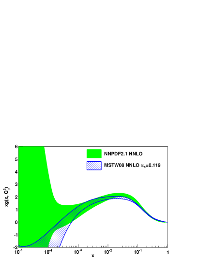
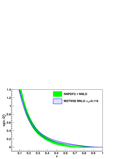
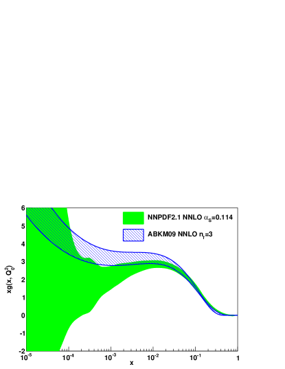
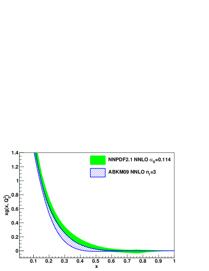
Figure 29: Comparison of the gluon density at $Q^{2}=2$ GeV² obtained in the NNPDF2.1, MSTW08 and ABKM09 NNLO analyses. The NNPDF2.1 density is shown for $\alpha_{s}=0.119$ ($\alpha_{s}=0.114$) in the top (bottom) row, such that it can be compared with the overlaid MSTW08 (ABKM09) density. Note that the ABKM uncertainties also include the uncertainty on $\alpha_{s}$ while for NNPDF and MSTW they are pure PDF uncertainties. From [220].

3.6.2 The convergence of perturbative series and low ${\boldsymbol{x}}$ effects

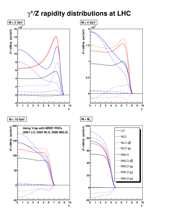
Figure 30: Drell-Yan cross section at the LHC in several mass bins, at LO, NLO and NNLO. From [223].

For processes that do not involve low $x$ partons, calculating the cross sections to LO, NLO and NNLO shows a reasonable convergence of the perturbative series. For example, the NNLO cross sections for $W$ and $Z$ production at the LHC, obtained from the NNLO MSTW08 PDFs, is only $3-4\%$ higher than the NLO cross section obtained from the NLO MSTW08 PDFs. However, for processes involving low $x$ partons, convergence may not be reached at NNLO. This is illustrated in Fig. 30 which shows the Drell-Yan cross sections at LO, NLO and NNLO, in four mass bins. For di-lepton masses smaller than a few $10$s of GeV, the NNLO and NLO predictions are largely different, even in the central region; the difference being larger for smaller masses. This may indicate that, in part of the kinematic range where the LHC experiments will make measurements (for example, LHCb should measure Drell-Yan at low masses in the rapidity range $2<y<5$, see chapter 4), a resummation of terms in $\ln(1/x)$ may be needed.

The measurement of the longitudinal structure function $F_{L}$ at HERA [123, 124] provides another test-bench for low $x$ effects that are not accounted for in the NNLO DGLAP equations. A resummed calculation was shown to best describe the data [224, 38]. However, as shown by Fig. 31, the fixed order DGLAP predictions are, in general, in reasonable agreement with the measurement, within the rather large uncertainties.

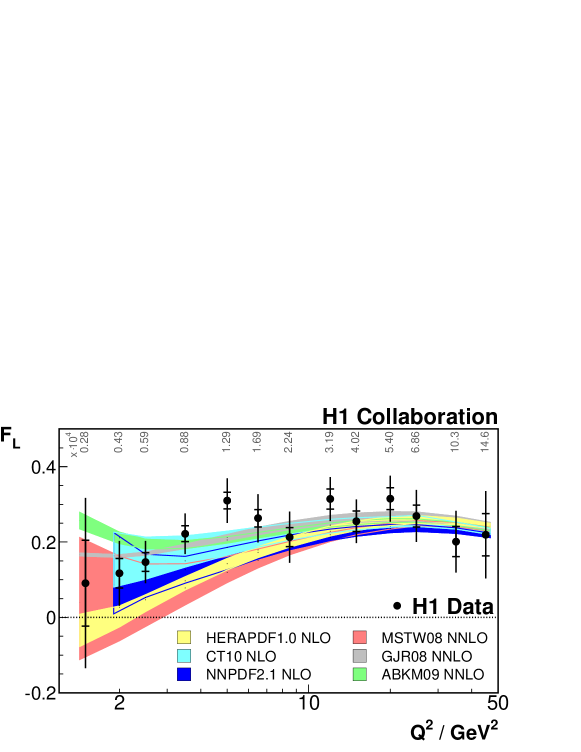
Figure 31: The longitudinal structure function $F_{L}$ measured by the H1 experiment, and compared with various NLO and NNLO predictions. From [123] .

The need for $\ln(1/x)$ resummations was also investigated by studying exclusive final states, such as forward pions or forward jets at HERA. The measurements were compared to fixed order DGLAP predictions, and to predictions based on the BFKL equation [225, 226], which involve un-integrated parton densities. No conclusive evidence for effects of BFKL dynamics was observed.

Besides resummations, the evolution of PDFs at very low $x$ is expected to be affected by saturation effects, due to parton recombinations. Saturation would lead to a taming of the rise of $F_{2}$ at low $x$. Such an effect has been looked for in HERA data, by investigating the slopes of $F_{2}$ [123], but was not observed in the $x$ and $Q^{2}$ range of the measurements. A possible hint for saturation in HERA data may come from the energy dependence of diffractive interactions, which was seen to be the same as that of the total cross section [227]. These aspects can be addressed within dipole models (see [228, 229] and references therein); a deeper discussion goes beyond the scope of this review.

4 PDF Constraints from the LHC

The LHC $pp$ collision physics programme is driven by the search for new physics and the understanding of electroweak symmetry breaking. Precise theoretical predictions of background processes are needed for a discovery, whereas accurate predictions of new phenomena are needed for the interpretation of exotic physics signals or for verification of the Higgs boson properties. This programme is now well under way with about $5$ fb^-1 of luminosity delivered to the ATLAS and CMS experiments in 2011, and more than $20$ fb^-1 at $\sqrt{s}=8$ TeV expected by the first long shutdown of the LHC in 2013. As discussed in section 2.4 measurements from the Tevatron $p\bar{p}$ collider provide important PDF constraints beyond those obtained from DIS data. Similarly it is expected that measurements from the LHC experiments will also improve our knowledge of proton structure.

4.1 The LHC experiments

The kinematic region opened up to the ATLAS, CMS and LHCb experiments in the initial phase of LHC operation at $\sqrt{s}=7$ TeV is shown in Fig. 32. The lowest $Q$ is set by available trigger thresholds and the lowest $x$ is determined by detector rapidity ($y$) acceptance. The ATLAS and CMS experiments are largely limited to $|y|<2.5$. For $W/Z$ production from partons with momentum fractions $x_{1}$ and $x_{2}$ (here, $x_{1}<x_{2}$ by convention) $M_{W,Z}^{2}=sx_{1}x_{2}$ and the boson rapidity is given by Eq. 32. This restricts the $x$ range at $\sqrt{s}=7$ TeV to approximately $10^{-3}<x<10^{-1}$. In contrast the LHCb experiment with more forward instrumentation is able to access the region $2<y<5$ which corresponds to $10^{-4}<x_{1}<10^{-3}$ and $0.1<x_{2}<1$ for the same $Q=M_{W,Z}$. The overall reach in $x$ will be extended by a further factor of two with $\sqrt{s}\simeq 14$ TeV operation expected by 2015.

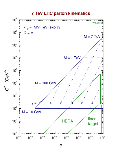
Figure 32: Kinematic phase space accessible at the LHC with $pp$ collisions at $\sqrt{s}$=$7$ TeV. From [230], adapted from [231].

4.1.1 The ATLAS and CMS detectors

The ATLAS [232] and CMS [233] detectors are designed as multi-purpose experiments to exploit the full physics potential at the LHC. They are segmented into a central barrel part and two endcap regions. The innermost part of the detectors consist of precision silicon pixel and strip tracking detectors close to the nominal interaction points providing charged particle momentum reconstruction over the region $|\eta|<2.5$. For ATLAS the silicon trackers are supplemented by a surrounding straw-tube transition radiation tracker for $|\eta|<2.0$ to enhance electron identification. Both detectors have a large solenoid field axial with the LHC beamline. The $2$ T field in the case of ATLAS encloses the tracking and the electromagnetic calorimeter, whereas the trackers, and both electromagnetic and hadronic calorimeters are immersed in the $3.8$ T field of CMS.

The ATLAS electromagnetic and hadronic calorimeters extend to $|\eta|<3.2$ and use a combination of liquid argon and tiled scintillator technologies as the active media for energy sampling. A very forward calorimeter provides additional coverage for $3.2<|\eta|<4.9$. The CMS electromagnetic and hadronic calorimeters use lead-tungstate crystals and scintillating plates for energy sampling respectively, in the region $|\eta|<3.0$, and are supplemented by an additional sampling Cherenkov calorimeter in the forward region covering $3.0<|\eta|<5.0$.

Muons are measured in detectors located outside of the magnet solenoids. The CMS design places the detectors inside a steel return yoke for the solenoid which provides a bending field for the muons and covers $|\eta|<2.4$. The ATLAS muon spectrometer uses three large superconducting toroid magnet systems and is able to measure muons over the range $|\eta|<2.7$.

4.1.2 The LHCb detector

The LHCb detector [234] is primarily designed to study properties of $B$-meson decays at the LHC, including $CP$ violation and observation of rare $B$ decays. It also has a programme of QCD and EW physics measurements which are of relevance to this article. The detector is a single arm forward spectrometer covering the region $2<\eta<5$. A precision silicon strip vertex detector is located close to the interaction region. Further strip silicon tracking devices are located on either side of a dipole magnet, supplemented by straw-tube tracking chambers. A ring imaging Cherenkov detector is used to help identify charged hadrons. Electromagnetic and hadronic calorimeters located downstream of the magnet distinguish electrons, photons and hadrons. Muons are detected in multi-wire proportional chambers furthest from the interaction region.

4.2 Benchmark cross section predictions

Parton luminosities are a convenient means of estimating the PDF contributions to, and the $\sqrt{s}$ dependence of hadronic cross sections for given combinations of partons [235]. The parton luminosity for the combination $\sum_{q}q+\bar{q}$ is relevant, for example, for $Z^{0}$ production, whereas the combination $gg$ is of importance for Higgs production at the LHC. Using Eq. 31, $\tau=x_{1}\cdot x_{2}=\hat{s}/s$ where $\hat{s}$ is the partonic centre-of-mass energy, the differential luminosities $\frac{\partial{\mathcal{L}}}{\partial\hat{s}}$ are defined as:

$$\frac{\partial{\mathcal{L}_{\sum q+\bar{q}}}}{\partial\hat{s}} = \frac{1}{s}\int^{1}_{\tau}\frac{dx}{x}\sum_{q}\left(f_{q}(x,\hat{s})f_{\bar{q}}(\tau/x,\hat{s})+[q\leftrightarrow\bar{q}]\right)$$

$$\frac{\partial{\mathcal{L}_{gg}}}{\partial\hat{s}} = \frac{1}{s}\int^{1}_{\tau}\frac{dx}{x}f_{g}(x,\hat{s})f_{g}(\tau/x,\hat{s})\,\,.$$ (56)

The ratio of several NLO parton luminosities to MSTW08 are compared in Fig. 33 where very good agreement between all sets is attained for the $W,Z$ resonance region, but diverge rapidly at higher or lower fractional partonic centre-of-mass energy. The level of agreement is similar for the $gg$ combination which shows a large spread of predictions which are in some cases outside the uncertainty bands of some of the predictions. This has led to a debate on the best way to estimate PDF uncertainties for cross section predictions incorporating the spread between PDF sets, and is discussed below.

A series of benchmark cross sections have been calculated at NLO and NNLO [236] in order to review the consistency of the most current PDF sets available (MSTW08, CTEQ6.6, CT10, NNPDF2.1, HERAPDF1.0, ABKM09 and GJR08). The chosen processes are $W$, $Z$ and $t\bar{t}$ production cross sections, as well as Higgs production with masses of $M_{H}=120,180,240$ GeV. The cross sections are determined for fixed values of $\alpha_{s}$.

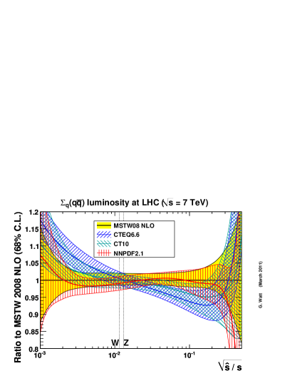
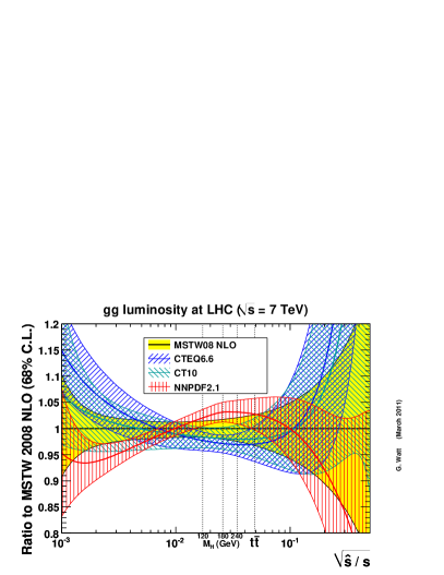
Figure 33: Parton luminosities for the LHC at 7 TeV for the combination $\sum_{q}q+\bar{q}$ (left) and $gg$ (right). From [236].

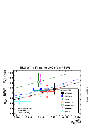
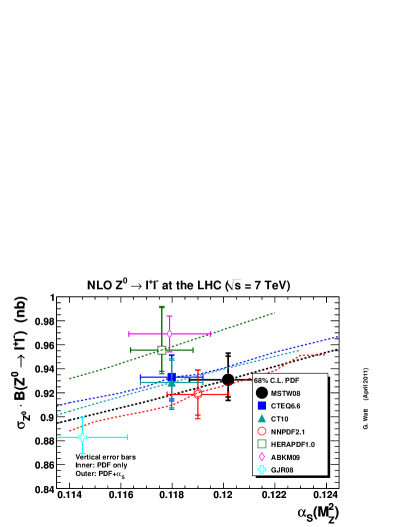
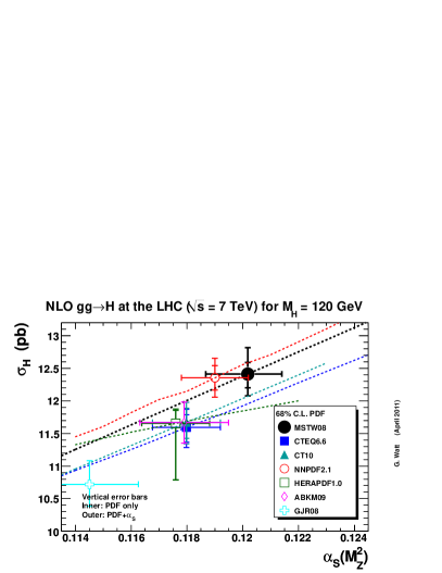
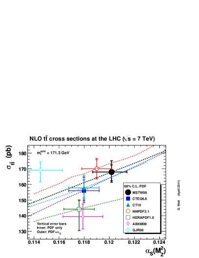
Figure 34: Predicted NLO cross sections for the LHC at $\sqrt{s}=7$ TeV for $W^{+}+W^{-}$ production (upper left), $Z^{0}$ production (upper right), $gg\rightarrow H$ for $M_{H}=120$ GeV (lower left) and $t\bar{t}$ production (lower right) with $68\%$ confidence level uncertainties as a function of $\alpha_{s}$. The inner vertical error bar corresponds to the PDF uncertainty and the outer error bar includes the $\alpha_{S}$ uncertainty. The horizontal error bar shows the $\alpha_{S}(M_{Z}^{2})$ range considered for the uncertainty. From [236].

An example of the NLO benchmark predictions is shown in Fig. 34. Each point is plotted at the value of $\alpha_{s}$ used in the central fit of the analysis. The dashed curves show the $\alpha_{s}$ variation using alternative PDFs from each group. The precision of the absolute cross section predictions at $68\%$ CL is broadly similar for each PDF set, i.e. $\sim 2-3\%$ for $W^{+}+W^{-}$ production and $\sim 2\%$ for $Z$ production. It is however apparent that these uncertainties do not fully cover the spread of predictions $\sim 6\%$. As expected the ratio of the $W^{+}+W^{-}$ and $Z$ cross sections (not shown) are obtained with greater precision and show a smaller spread. This is due to the fact that the numerator and denominator of the ratio are both largely sensitive to the PDF combination $u+d$, and that the $\alpha_{s}$ dependence almost cancels.

In addition to these variations the theoretical uncertainty should also take into consideration the effects of neglected higher-orders. These are usually estimated by varying the $\mu_{F}$ and $\mu_{R}$ scales within a factor of two of the default choice usually taken to be $\mu_{F}=\mu_{R}=M_{Z,W,H}$. The influence of the scale uncertainty depends on the cross section under study, and can be $~{}3\%$ for $Z$ production at NLO but is dramatically reduced to $0.6\%$ at NNLO [236].

Production of $t{\bar{t}}$ pairs at the LHC for $\sqrt{s}=7$ TeV is dominated by $gg$ initial states which account for $80\%$ of the production cross section and at threshold probes $x\sim 2m_{t}/\sqrt{s}=5\times 10^{-2}$ [236]. By contrast $W$ and $Z$ resonant production is dominated by $q{\bar{q}}$ pairs probing $x\sim 2\times 10^{-2}$. Thus $W,Z$ cross sections are anti-correlated with $t{\bar{t}}$ production since an enhanced gluon distribution at higher $x$ would lead to a reduced quark distribution at lower $x$ through the sum rules [231]. The predictions for $t{\bar{t}}$ production are as yet only approximately known at NNLO. The predictions with different PDF sets [236] are calculated at NLO and NNLO and show considerable range of about $\pm 10$% which is larger than the uncertainties estimated from a single PDF set at $68\%$ CL. The $90\%$ CL uncertainty bands give a better reflection of the variation in the predictions.

In Fig. 35 a comparison of production cross sections for the SM Higgs boson is shown (as a ratio to the MSTW08 prediction) for a range of $M_{H}$. The NLO predictions each have an uncertainty of $\pm 3\%$ (at $68\%$ CL and including the uncertainty on $\alpha_{s}$) although the spread between different PDF sets can be as large as $10\%$. At NNLO the uncertainty bands are marginally larger, and the spread of predictions is considerably larger than at NLO. However, scale uncertainty is not included in the error bands shown, and is reduced by a factor of two to about $9\%$ at NNLO [237, 238].

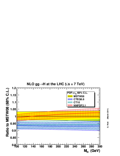
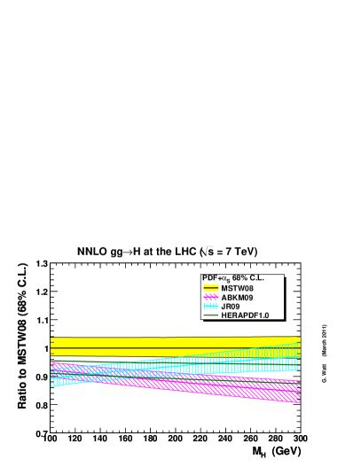
Figure 35: Predicted cross sections at NLO (left) and NNLO (right) for Higgs production with $68\%$ confidence level uncertainties as a function of $M_{H}$. The ratio to MSTW08 prediction is shown. From [236].

These studies have been discussed in detail within the PDF4LHC working group [239]. The group has made a recommendation on how to determine NLO and NNLO PDF uncertainties for cross section predictions which takes into account the spread between the PDF groups [240]. At NLO the prescription is based on the MSTW08, CTEQ6.6 and NNPDF2.0 PDF sets which are commonly used by the LHC experiments (although now CTEQ6.6 is superceded by CT10, and NNPDF2.0 by NNPDF2.3). The recommendation is to calculate the envelope of the three group’s PDF $+\alpha_{s}$ uncertainty, and the mid-point taken as the central value. At NNLO the recommendation is based on the MSTW08 PDFs where the uncertainty of this set is increased by a scale factor obtained from the ratio of the NLO PDF4LHC uncertainty band to the MSTW08 NLO error band. This factor is found to be $\sim 2$ for the $gg\rightarrow H$ process at the LHC.

It is argued [236] that the prescription given above may be overly complex to apply to all processes, for example in a process where the theoretical uncertainty is dominated by scale variations. In some cases it may be easier and statistically more correct to evaluate the uncertainties according to the prescription of one PDF group using the $90\%$ CL uncertainty. For example the NNLO uncertainties evaluated using the MSTW08 PDFs (and their prescription) including scale uncertainties, $\alpha_{s}$ variations and the choice of $b$ and $c$ quark masses are found to be ${}^{+2.9}_{-2.4}\%$ and ${}^{+5.0}_{-4.7}\%$ for $Z$ production production at $68$% and $90$% CL respectively.

4.3 First LHC measurements

4.3.1 Electroweak measurements

The initial measurements of the $W$ and $Z$ production total and differential cross sections have now been published by ATLAS [241], CMS [242, 243, 244] and LHCb [245]. The $Z$ production cross section is sensitive to the dominant combinations $u{\bar{u}}+d{\bar{d}}+s{\bar{s}}$, whereas $W^{+}$ probes $u{\bar{d}}+c{\bar{s}}$ and $W^{-}$ probes $d{\bar{u}}+s{\bar{c}}$. Thus the flavour structure of the proton is accessible via measurements of $W^{+}$ and $W^{-}$ production, or through the $W$ lepton charge asymmetry $A(\eta)$:

$$A(\eta)=\frac{{\rm d}\sigma/{\rm d}\eta(W^{+}\rightarrow l^{+}\nu)-{\rm d}\sigma/{\rm d}\eta(W^{-}\rightarrow l^{-}{\bar{\nu}})}{{\rm d}\sigma/{\rm d}\eta(W^{+}\rightarrow l^{+}\nu)+{\rm d}\sigma/{\rm d}\eta(W^{-}\rightarrow l^{-}{\bar{\nu}})}$$ (57)

which have recently been published [241, 245, 246, 247, 248]. The most precise measurements of the asymmetry in $p{\bar{p}}$ collisions from D0 show some tension with the CDF measurements and to some extent with other DIS data (see 3.5.1). At the LHC the spread of predictions for this observable can be as much as a factor of two larger than the $90\%$ CL uncertainty from MSTW08[236]. Fits to the di-muon production data in $\nu$ and $\bar{\nu}$ induced DIS prefer an enhanced $s$ compared to $\bar{s}$ contribution (see section 3.5.5), although the significance of this finding is weak. Since the contribution of $s/{\bar{s}}$ to $Z$ and $W$ production is large at the LHC (up to $20$% and $27$% respectively at NLO [249]) new LHC data could help resolve the issue and set interesting constraints in the strange sector. First studies were carried out in [250] and pursued in [213].

$\boldsymbol{W}$ and $\boldsymbol{Z}$ cross sections

First measurements of the $W$ and $Z$ production cross sections in $e$ and $\mu$ decay channels at $\sqrt{s}=7$ TeV are available  [241, 242, 245] using $\sim 35$ pb^-1 integrated luminosity recorded in 2010. The measurements are systematically limited and both experiments have a precision of $\sim 1\%$ (excluding a $3-4\%$ luminosity uncertainty). Fig. 36 shows the correlation of the $W^{+}$ to $W^{-}$ production cross sections, and the $W^{+}+W^{-}$ to $Z$ production from ATLAS. NNLO predictions compare favourably with the measurements within their quoted uncertainties.

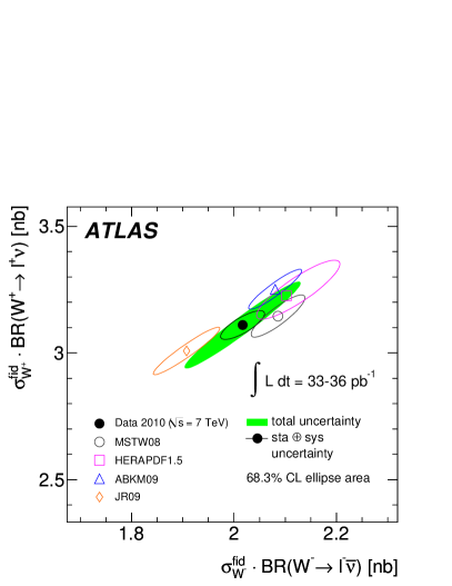
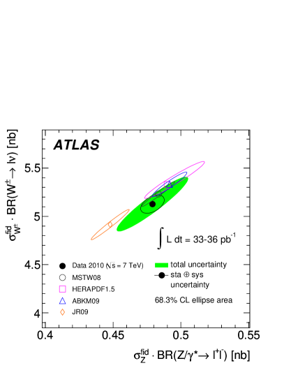
Figure 36: The measured and predicted production cross sections times branching ratio for $W^{+}$ vs. $W^{-}$ production (left), and for $W$ vs. $Z$ production (right). From [241].

Differential Drell-Yan measurements

The virtual $\gamma^{*}$ cross section below the $Z$ resonance provides complementary information to that obtained at the $Z$ peak. At low $\gamma^{*}$ invariant mass the electromagnetic couplings dominate which suppress the $d$-type contributions whereas the axial and vector EW couplings to the $u$ and $d$ quarks, $v^{2}+a^{2}$, are of similar size (see Eq. 42). Thus measurements at the $Z$ resonance peak and of the low mass continuum are sensitive to different combinations of $u$-type and $d$-type quarks.

Since the virtual boson rapidity is related to the ratio of the quark and anti-quark parton momentum fractions, an interesting measurement is the $y$ spectrum in $Z/\gamma^{*}$ interactions. At large $y$ the longitudinally boosted boson arises from increasingly asymmetric momentum fractions of the $q,{\bar{q}}$ pair which provides simultaneous access to the high $x$ and low $x$ kinematic regions. Measurements of the low mass Drell-Yan cross section reach the region of very low $x\sim~{}10^{-4}$ for ATLAS and CMS, and $10^{-5}$ for LHCb. At very low mass however, fixed order calculations are not yet stable (see 3.6.2). The PDF uncertainty for $M\sim 15$ GeV is estimated to be $3\%$ at NLO but the scale uncertainty can lead to variations of as much as $30\%$ on the cross section (taking $\mu_{F}=\mu_{R}={\hat{s}}$) which rapidly diminishes with increasing $M$, and could limit the use of the lowest $M$ data in PDF fits. At NNLO the scale uncertainty remains sizeable at about $4\%$ but can be reduced by choosing the scale appropriately such that the higher order contributions are minimised [251].

The first measurements of the differential invariant mass spectrum from CMS [244] are shown in Fig. 37 (left) spanning the range $15<M<600$ GeV compared to NNLO predictions. Preliminary measurements from LHCb down to $M=6$ GeV are also released [252]. Both measurements are based on the 2010 datasets and have a moderate precision of $9\%$ at $M=15-20$ GeV which is expected to improve.

Differential spectra for $W$ and $Z$ production have been published by ATLAS [241], CMS [243] and LHCb [245] and the LHCb measurements are shown in Fig. 37 (right) compared to NNLO predictions. The data, which in this case are based on the statistically limited 2010 data sample, are not yet of sufficient precision to significantly constrain the PDFs although some deviation between theory and measurement is observed for $2.5<y<3.0$. It will be interesting to see how this develops with the new measurements with higher statistical precision and smaller systematic uncertainties.

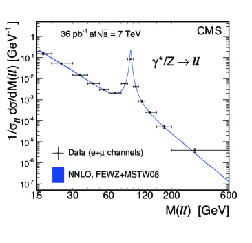
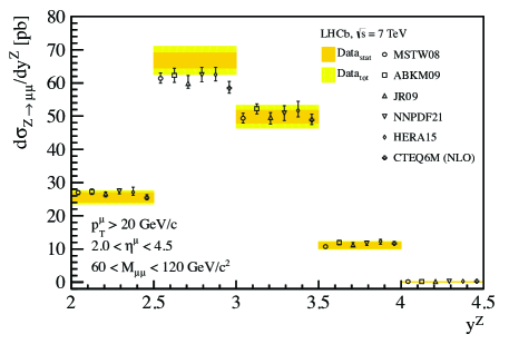
Figure 37: Left: The normalised differential Drell-Yan cross section vs. invariant mass of the virtual boson. Right: the differential rapidity spectrum of $Z^{0}$ production. From [244, 245].

$\boldsymbol{W}$ charged lepton asymmetry

Measurements from ATLAS, CMS and LHCb of the $W$ charged lepton ($e+\mu$) asymmetry are presented in [241, 246, 247, 248, 245]. Fig. 38 shows the asymmetry as determined by all three experiments compared to fixed order NLO and NNLO predictions from several PDF groups. The CMS electron channel measurement is shown in Fig. 38 (left) using $840$ pb^-1 of integrated luminosity with a lepton $p_{T}$ cut of $35$ GeV. The data are in good agreement with most NLO predictions, but at low lepton rapidity $\eta_{l}$ the MSTW08 prediction undershoots the data. The differences between PDF sets are more pronounced in the predicted $W^{+}$ and $W^{-}$ rapidity spectra leading the authors of [241] to argue that the individual spectra are more sensitive than the lepton charge asymmetry. Better agreement between predictions and measurements may be obtained when comparing to resummed calculations at next-to-next-to-leading log order since these calculations give a better description of the the $W$ $p_{T}$ spectrum as pointed out in [247].

The charged lepton asymmetry measurements from ATLAS, CMS and LHCb are shown together in Fig. 38 (right) based on a smaller data set of $35-36$ pb^-1 and less restrictive phase space with the lepton $p_{T}$ required to be above $20$ GeV. The NLO predictions of CTEQ6.6, HERAPDF1.0 and MSTW08 are in reasonable agreement with the data shown, although here, better agreement with MSTW08 is observed albeit within larger experimental uncertainties. Of particular interest is the region accessed by the LHCb measurement for $\eta_{l}>2.5$ where the predictions are in agreement with each other and the data but with relatively large uncertainties. Thus current and future measurements are expected to have a visible impact in reducing the PDF uncertainties and improving the consistency between PDF sets at large and small $\eta_{l}$.

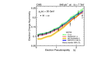
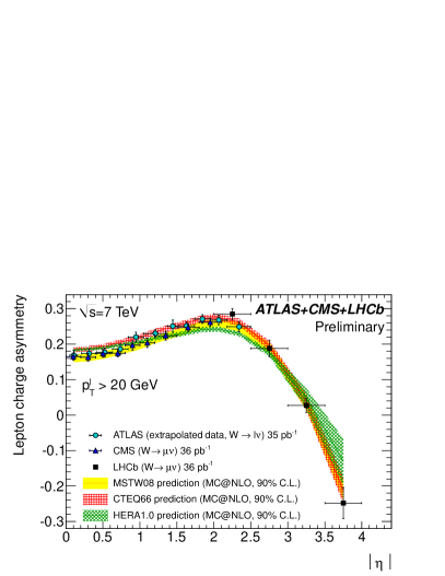
Figure 38: Charged lepton asymmetry in $W$ decays at the LHC. Left: CMS electron measurement for $p_{T}>35$ GeV with $840$ pb^-1 from [248]. Right: combined electron and muon channel measurements from ATLAS, CMS and LHCb for $p_{T}>20$ GeV with $35-36$ pb^-1 from [253].

4.3.2 Inclusive jet cross sections

Differential inclusive jet cross sections $d^{2}\sigma/dydp_{T}$ at $\sqrt{s}=7$ TeV are available from ATLAS [254] and CMS [255] and an example of the data can be seen in Fig. 39. Even with the modest luminosity of $\sim 35$ pb^-1 the measurements extend to jet transverse momenta of about $1.5$ TeV. The wide $\eta$ range of the ATLAS and CMS calorimeters compared to the Tevatron experiments allows the jet cross sections to be measured up to high rapidities of $4.4$. The measurements are sensitive to partonic momentum fractions $x$ of $\sim 10^{-5}<x<0.9$, however the precision is limited by the knowledge of the detector calibration. Jet cross sections exhibit a very sharply falling jet $p_{T}$ spectrum (see for example Fig. 13), therefore small changes in the jet energy scale lead to large correlated shifts in the cross sections. Currently this leads to measurement uncertainties of about $10-60\%$ dominated by a scale uncertainty of $3-4\%$ in the central detector regions for moderate jet $p_{T}$ and rising to $\sim 12\%$ at the highest $y$.

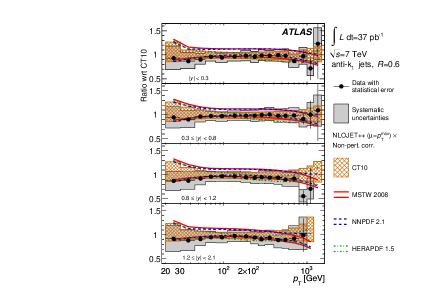
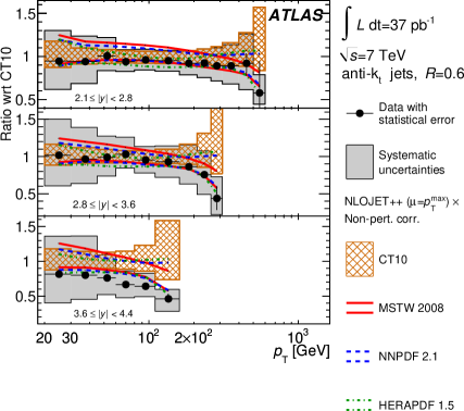
Figure 39: Ratio of the measured inclusive jet cross section $d^{2}\sigma/dydp_{T}$ to the theoretical prediction using CT10 PDFs. The predictions from MSTW08, NNPDF2.1 and HERAPDF1.5 are also shown. From [254].

4.3.3 The NNPDF2.3 PDFs

Global fits that include the early LHC measurements described above have been performed by the NNPDF collaboration.

In [256], the NNPDF2.1 NLO PDFs were updated using a reweighting technique to include the first $W$ charged lepton asymmetry measurements from ATLAS and CMS, leading to the NNPDF2.2 set.

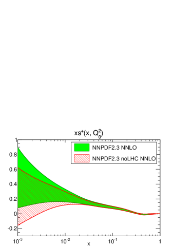
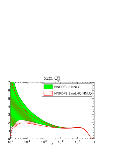
Figure 40: Comparison of the strangeness and singlet distributions obtained from NNPDF2.3, which includes the LHC data, and from the same fit but restricted to the non-LHC measurements. The contours correspond to uncertainties at $68\%$ confidence level. From [213].

In [213] new fits were performed which include, in addition to the non-LHC data used in NNPDF2.1, the published measurements from the LHC experiments for which the covariance matrix of the correlated systematic uncertainties has been provided: the $W$ and $Z$ lepton rapidity distributions measured by ATLAS [241] and LHCb [245] using the 2010 data, the $W$ electron asymmetry measured by CMS in the 2011 dataset [248], and the ATLAS inclusive jet cross sections measured in the 2010 data [254]. The corresponding NNPDF2.3 PDFs have been determined both at NLO and at NNLO for a wide range of values of $\alpha_{s}$, in the same GM-VFNS scheme as used for NNPDF2.1, and are available in the LHAPDF interface. For the determination of NNLO PDFs, the NNLO predictions for electroweak boson production at the LHC have been obtained via K-factors. For inclusive jet production at the LHC, the NLO matrix elements have been used (together with NNLO PDFs and $\alpha_{s}$) instead of the approximation usually made to calculate NNLO jet production at the Tevatron (see section 3.6), because the threshold approximation is expected to be worse at the LHC energies.

The resulting NNPDF2.3 distributions provide a good description of all datasets included in the fit. The comparison of these PDFs with those obtained from the same fit performed to the non-LHC data only (the NNPDF2.3-noLHC set already mentioned at the beginning of 3.5) allows to gauge the specific impact of the LHC data. This impact is so far moderate but already visible [213]: the uncertainty on the gluon distribution at high $x$ is somewhat reduced thanks to the LHC jet data; the electroweak boson production data help improve the flavour decomposition; and the strangeness fraction of the light sea is pushed towards slightly higher values, although with a marginal statistical significance. As an example, Fig. 40 compares the strange and singlet distributions obtained from NNPDF2.3 and NNPDF2.3-noLHC.

PDF fits based only on collider data

PDFs derived from a fit restricted to data from collider experiments were also extracted in [213]. The motivation of this approach lies in the fact that the resulting PDFs are, by construction, independent of any nuclear or higher twist corrections that may affect some fixed target measurements, and could explain some of the tensions reported in 3.5.6. Restricting the fit to the collider measurements reduces by a factor of $\sim 3$ the number of fitted data points. The resulting PDFs show no significant differences with those from NNPDF2.3, which indicates that any tension between collider and fixed target data can only be moderate. However, some distributions resulting from this fit show very large uncertainties. For example, the anti-quark PDFs at high $x$ are very poorly constrained in such a fit, as shown by the dashed curves in Fig. 26 of section 3.5.3.

4.3.4 Top production

The production of $t\bar{t}$ pairs is dominated by $gg$ fusion at the LHC, and at $\sqrt{s}=14$ TeV this subprocess contributes $90\%$ of the total cross section. Therefore this provides an interesting probe of the high $x$ gluon particularly at large $t\bar{t}$ invariant mass $>1$ TeV. However, care should be taken in interpreting these cross sections which are also used to constrain many models of new physics coupling to the top quark.

Latest measurements of the total production cross section based on $7$ and $8$ TeV centre-of-mass energy data from ATLAS and CMS have been reported in a variety of decay modes including single and di-lepton $W$ decays as well as purely hadronic modes, and measurements using $b$ tagged jets, for example [257, 258, 259, 260, 261] and references therein. The latest combination of measurements are presented in [262, 263] and an experimental precision of $\sim 5\%$ is now achieved (excluding the luminosity uncertainty). Recent approximate NNLO predictions [264] and NLO predictions with next-to-next-to-leading log (NNLL) corrections [265] both have a similar accuracy of about $\pm 4\%$ for the scale variation uncertainty and $\pm 5\%$ for the PDF uncertainty evaluated using only the MSTW08 NNLO set at $90\%$ CL. This estimated PDF uncertainty is smaller than the spread of different predictions as discussed in 4.2, and the measurements are expected to constrain the differences between the PDF sets.

A first measurement of the normalised differential $t\bar{t}$ cross section is now available performed with a $2$ fb^-1 data sample at $\sqrt{s}=7$ TeV [266] in the single lepton ($e$+$\mu$) channel. The data are shown in Fig. 41 and compared to NLO and NLO+NNLL predictions. A precision of $10-20\%$ is achieved which is limited by uncertainties related to the jet energy scale and resolution.

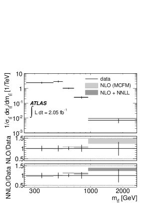
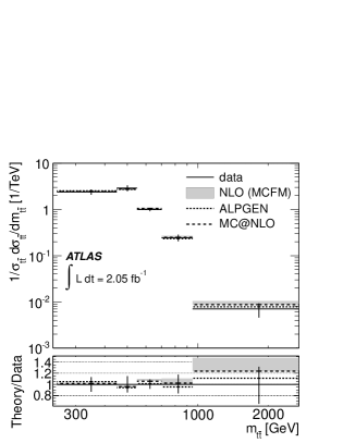
Figure 41: Normalised $t\bar{t}$ differential cross section at $\sqrt{s}=7$ TeV compared to four NLO and NLO+NNLL predictions. From [266].

4.3.5 Prompt photon production

The potential sensitivity of measurements of isolated photon hadro-production on the gluon density has been mentioned in section 2.4.4, in the context of pre-LHC experiments. In $pp$ collisions at the LHC, the relative contribution of the QCD Compton process $qg\rightarrow\gamma q$ to prompt photon production is enhanced compared to what happens in $p\bar{p}$ collisions at the Tevatron, where $q\bar{q}$ annihilations $q\bar{q}\rightarrow\gamma g$ also play an important role. Moreover, in the large kinematic domain where the measurement can be performed at the LHC, the gluon density is involved in a broad range of Bjorken-$x$, from ${\cal{O}}(10^{-3})$ at rapidities of $|\eta|\simeq 2$ and low transverse energy to ${\cal{O}}(0.1)$ at central pseudo-rapidities and high $E_{T}$ [170]. Hence, the impact of LHC prompt photon measurements on the gluon PDF is expected to be significant.

First measurements of isolated prompt photon production have been published by the ATLAS [267] and CMS [268] experiments using $pp$ data taken at $\sqrt{s}=7$ TeV corresponding to an integrated luminosity of $\sim 35$ pb^-1. For example, the CMS measurement, made in four pseudo-rapidity regions and in the transverse energy range $25<E_{T,\gamma}<400$ GeV, is shown in Fig. 42. It is consistent with the NLO prediction from pQCD obtained from the JETPHOX program [270, 271] using the CT10 PDFs.

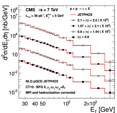
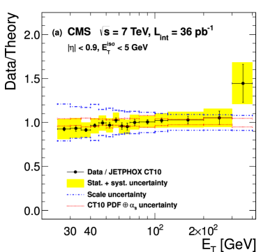
Figure 42: Left: The isolated prompt photon cross section measured in four pseudo-rapidity bins as a function of the photon transverse energy, together with the NLO QCD prediction. Right: Ratio of the measurement to the NLO prediction for the most central bin; the vertical error bars show the statistical uncertainties, while the shaded areas show the total errors (not including a $4\%$ normalisation uncertainty). From [268].

In [170], the impact of these ATLAS and CMS data on the PDFs has been quantified using the NNPDF reweighting technique mentioned previously [256]. Including these data in a fit similar to NNPDF2.1 leads to a significant reduction of the uncertainty on the gluon PDF, of up to $20\%$, most pronounced for $x\sim 0.01$. Moreover, the fit does not change significantly the central value of the gluon density. This indicates that the constraints that these data set on the gluon PDF at high $x$ have no tension with the constraints obtained from the Tevatron jet data.

4.3.6 Cross section ratios

The centre-of-mass energy of the LHC is being increased in a step-wise way with runs taken at $\sqrt{s}=7$ TeV and $8$ TeV and after the long shutdown in 2013-2014, the machine is expected to operate at $\sim 14$ TeV. This gives rise to the possibility of measuring cross section ratios at different $\sqrt{s}$ as well as double ratios of hard process cross sections. The advantage of these ratios is that experimentally many systematic uncertainties could cancel in the measurements. Cancellation in the theoretical uncertainties on the predictions are also expected [272] leading to very precise predictions and measurements. These could offer interesting new constraints on PDFs and enhanced sensitivity to new physics. Taking the ratio between the $7$ and $8$ TeV data the $W$ and $Z$ production cross section ratios are predicted to an accuracy of $\sim 0.2\%$ including PDF, $\alpha_{s}$, and scale uncertainties at NNLO. However, for high mass $t{\bar{t}}$ production the predicted uncertainty on the ratio is estimated to be $1\%$, and jet production ratios for jets with $p_{T}>1$ TeV are claimed to be known to $\sim 2\%$, rising to $\sim 6\%$ for jet $p_{T}>2$ TeV. Both of these processes probe the very high $x$ PDFs and could therefore be used to constrain this region. The ratios between $8$ and $14$ TeV data offer even larger potential gains. It remains to be seen how well the experimental uncertainties on the measured ratios will cancel but this is an interesting proposal warranting further more detailed investigations.

5 Conclusions and Outlook

A lot of progress has been made over the past $\sim 20$ years in the understanding of proton structure and in the determination of the parton distribution functions. On the experimental side, the HERA collider has opened up the kinematic domain of low $x$; high $p_{T}$ jet production at the Tevatron has shed light on the gluon density at high $x$; the measurements from fixed target experiments have been finalised. On the theory side, the extraction of PDFs has become more and more involved. While the first QCD fits were made at leading order only, to a small number of $F_{2}$ data points, using simple parameterisations with a few parameters, current QCD fits are now available up to NNLO; they make use of about $3000$ data points, covering all processes that are sensitive to proton PDFs; the parameterisations have typically $25-30$ parameters (ten times more for the NNPDF fits); and uncertainties are now delivered together with the central fits. The crucial need for obtaining error bands for the PDFs has also lead the experimental collaborations to publish their full correlated systematic uncertainties. This much improved knowledge of proton structure comes together with lots of progress in QCD phenomenology and theory: thanks to new calculation techniques, higher order calculations are now available for a wealth of processes; several resummed calculations also exist; the development of new subtraction techniques has allowed NLO calculations to be combined with the parton shower approach used in Monte-Carlos; new jet algorithms have been defined, that allow to better compare experimental measurements with theoretical calculations. As a result, the theoretical predictions for the processes that are, or will be, observed at the LHC, are much more robust than what they were one decade ago, at the start-up of the Run II of the Tevatron.

Although most proton PDFs are now determined to a good precision, some open issues remain. For example, the strange content of the proton is still very poorly known, all PDFs are affected by large uncertainties at high $x$, and what happens at very low $x$ remains largely unknown. The data that are being collected by the LHC experiments will further improve our knowledge of proton structure - although the highest mass domain, which may be affected by physics processes not accounted for in the Standard Model, may not be best suited to constrain the PDFs at highest $x$.

In addition, other aspects of proton structure, which were not addressed in this review, are far from being understood. The proton spin is one of those. Since the surprising finding by the EMC Collaboration that very little of the proton spin is carried by the spins of quarks and anti-quarks, this issue has been tackled by several experiments, as (to mention only the most recent ones) the COMPASS experiment at CERN, HERMES at DESY, CLAS at JLab, and the STAR and PHENIX experiments at RHIC. One of the focus was the measurement of the contribution to the proton spin that is carried by gluons. There is currently no experimental evidence that this contribution may be important, however the uncertainties are large. Another issue regards the transverse structure: the standard PDFs probe the longitudinal momentum of the partons in a fast moving hadron, all information about the transverse structure is integrated over. This additional information is encoded within the Generalised Parton Distributions (GPDs), which unify the concept of PDFs and that of hadronic form factors [273]. The GPDs, which can be accessed via exclusive processes as Deep Virtual Compton Scattering $lp\rightarrow lp\gamma$, are poorly constrained so far.

The study of proton structure has a continuing programme over the next decade with, besides the LHC experiments, several new experiments and facilities in the planning, construction or starting phase. Some of these are designed to focus on the high $x$ region at low and moderate $Q^{2}$ whereas others are designed to open a wider kinematic region than is currently accessible. They are briefly described below.

The Minerva experiment (E938) at Fermilab [274]

The Minerva detector is operated on the NuMI neutrino beamline. Its main goal is to perform precision measurements of neutrino scattering off several targets in the low energy regime, $E_{\nu}\sim 1-20$ GeV, which are needed by experiments studying neutrino oscillations. Following a low-energy run which ended in May $2012$, data taken starting from $2013$ with a higher energy beam will allow CC DIS to be further studied. The measurements should shed further light on the $d/u$ ratio at high $x$.

The Drell-Yan experiment E906/Seaquest [275]

This Fermilab experiment continues the series of fixed target $pp$ and $pd$ Drell-Yan measurements from E605, E772 and E866. Seaquest will operate with a $120$ GeV proton beam delivering an instantaneous luminosity of $10^{35}$ cm^-2s^-1, some $50$ times the luminosity of E866. This will allow measurements of the $\bar{d}/\bar{u}$ ratio to be made with a factor $10$ improvement in precision in the region of $0.25<x<0.45$. The experiment will commence physics runs in 2013.

The COMPASS experiment at CERN

has a programme extending until $2016$ (see [276]). In particular it will perform further measurements of DVCS in $2015-2016$ (this requires major rearrangements of the spectrometer and the installation of a recoil detector). Measuring the dependence in $t$, the momentum transferred at the proton vertex, will give access to the nucleon transverse size. Combined with the HERA data and the future JLab data (see below), a comprehensive picture of the evolution of the nucleon’s transverse size with $x_{Bjorken}$ will be achieved. Information on GPDs will also be obtained.

The upgrade of the accelerator complex at JLab[277]

The Jefferson laboratory hosts the CEBAF dual linac electron accelerator currently operating at $6$ GeV delivering beam to three experimental halls. The machine is being upgraded to operate at $12$ GeV and instantaneous luminosities of $10^{35}-10^{39}$ cm^-2s^-1 which is necessary to explore the region of high $x\sim 0.7$ and $Q^{2}\lesssim 8$ GeV². Each hall houses one or more experiments and a fourth hall is under construction. The experiments cover a variety of measurements of nuclear and proton DIS including precision measurements of $F_{L}$ and $F_{2}$ at high $x$, measurements of $F_{2}$ neutron which will constrain the $d/u$ quark ratio at high $x$, DVCS measurements, as well as polarised scattering. The staged upgrade programme is underway and expected to commence physics operation in $2015$.

The Electron Ion Collider [278]

At the horizon of $\sim 2020$, a future EIC could be realised as an upgrade to the existing RHIC ion collider (eRHIC). A $5-30$ GeV polarised electron beam would collide with polarised ion beams reaching a maximum of $325$ GeV for protons, and $130$ GeV/A for heavier nuclei. Another option (MEIC / ELIC) would be to use the polarised electron beam of JLab and add a new ring for polarised protons or ions. The EIC would be the first lepton-proton collider with a polarised proton beam. It would shed further light on the proton’s spin problem. The contribution of gluons to the proton’s spin will be measured precisely by an EIC. If this contribution turns out to be small, as indicated by the current experimental data, it would mean that a large part of the proton spin is due to orbital angular momentum. The measurement of DVCS and of other exclusive processes as $J/\psi$ production, off transversely polarised protons, will bring information on GPDs at low $x$. Together with the information on GPDs obtained, at higher $x$, by other experiments, it may then be possible to have a direct access to the parton angular momentum via Ji’s angular momentum sum rule [279] (this requires the GPDs to be reconstructed in a large kinematic domain). Moreover, the EIC physics programme also includes measurements of unpolarised proton and deuteron scattering at low $x$, measurements of $F_{L}$, and semi-inclusive DIS measurements sensitive to $s/\bar{s}$ content of the proton.

The LHeC project [280]

This is a novel proposal to build a ring or linac electron machine to collide with an LHC proton/ion beam using interaction point IP2 in the LHC tunnel. The LHC and LHeC could run simultaneously with operation commencing in 2023 or later, after the long shutdown in preparation for LHC high luminosity running. The electron ring operating at $60$ GeV and $\sqrt{s}=1.3$ TeV could offer a luminosity of $10^{33}$ cm^-2s^-1, a factor $20$ higher than HERA. A linac option could achieve higher $\sqrt{s}$ but the luminosity at these higher energies would be smaller. The physics programme would cover the measurement of precision NC and CC structure functions with a $20$-fold increase in kinematic reach for $Q^{2}$ and $1/x$ compared to HERA, improved accuracy in the determination of $\alpha_{s}$, and the understanding of saturation and of non-linear dynamics.

The long term future of DIS experiments is not yet clear with the last two projects described above still being discussed within the appropriate committees. Nevertheless, our knowledge of proton structure and QCD is expected to improve significantly within the next decade, alongside more general developments across the field of particle physics. Such developments will come in particular from the LHC experiments which, at the time of writing, have just announced the discovery of a new particle in their searches for the Standard Model Higgs boson.

References

- [1] E. Rutherford, Phil. Mag. 21 (1911) 669.
- [2] N. F. Mott, Proc. R. Soc. A 124 (1929) 422.
- [3] M. E. Rose, Phys. Rev. 73 (1948) 279.
- [4] M. N. Rosenbluth, Phys. Rev. 79 (1950) 615.
- [5] R. Hofstadter and R. W. McAllister, Phys. Rev. 98 (1955) 217.
- [6] E. E. Chambers and R. Hofstadter, Phys. Rev. 103 (1956) 1454.
- [7] B. Hahn, D. G. Ravenhall and R. Hofstadter, Phys. Rev. 101 (1956) 1131.
- [8] G. Zweig, “Developments In The Quark Theory Of Hadrons”, vol. 1, 22-101, eds. D.B. Lichtenberg and S.P. Rosen; CERN Geneva - TH. 401 (REC.JAN. 64) 24p.
- [9] M. Gell-Mann, Phys. Lett. 8 (1964) 214.
- [10] D. H. Coward et al., Phys. Rev. Lett. 20 (1968) 292.
- [11] M. Goitein, R. J. Budnitz, L. Carroll, J. Chen, J. R. Dunning, K. Hanson, D. Imrie and C. Mistretta et al., Phys. Rev. Lett. 18 (1967) 1016.
- [12] K. Berkelman, M. Feldman, R. M. Littauer, G. Rouse and R. R. Wilson, Phys. Rev. 130 (1963) 2061.
- [13] W. Albrecht, H. -J. Behrend, H. Dorner, W. Flauger and H. Hultschig, Phys. Rev. Lett. 18 (1967) 1014.
- [14] WAlbrecht, H. J. Behrend, F. W. Brasse, W. Flauger, H. Hultschig and K. G. Steffen, Phys. Rev. Lett. 17 (1966) 1192.
- [15] W. Bartel, B. Dudelzak, H. Krehbiel, J. M. McElroy, U. Meyer-Berkhout, R. J. Morrison, H. Nguyen-Ngoc and W. Schmidt et al., Phys. Rev. Lett. 17 (1966) 608.
- [16] T. Janssens, R. Hofstadter, E. B. Hughes and M. R. Yearian, Phys. Rev. 142 (1966) 922.
- [17] E. D. Bloom et al., Phys. Rev. Lett. 23 (1969) 930.
- [18] M. Breidenbach et al., Phys. Rev. Lett. 23 (1969) 935.
- [19] S. D. Drell and J. D. Walecka, Annals Phys. 28 (1964) 18.
- [20] J. D. Bjorken, Phys. Rev. 179 (1969) 1547.
- [21] R. P. Feynman, Phys. Rev. Lett. 23 (1969) 1415.
- [22] J. D. Bjorken and E. A. Paschos, Phys. Rev. 185 (1969) 1975.
- [23] C. G. . Callan and D. J. Gross, Phys. Rev. Lett. 22 (1969) 156.
- [24] D. J. Gross and F. Wilczek, Phys. Rev. Lett. 30 (1973) 1343.
- [25] H. D. Politzer, Phys. Rev. Lett. 30 (1973) 1346.
- [26] F. J. Hasert et al. [Gargamelle Neutrino Collaboration], Phys. Lett. B 46 (1973) 138.
- [27] H. Deden et al. [Gargamelle Neutrino Collaboration], Nucl. Phys. B 85 (1975) 269.
- [28] D. J. Fox, C. Chang, K. W. Chen, A. Kotlewski, P. F. Kunz, L. N. Hand, S. Herb and S. C. Loken et al., Phys. Rev. Lett. 33 (1974) 1504.
- [29] R. Brandelik et al. [TASSO Collaboration], Phys. Lett. B 86 (1979) 243.
- [30] J. Ashman et al. [European Muon Collaboration], Phys. Lett. B 206 (1988) 364.
- [31] B. Adeva et al. [Spin Muon Collaboration], Phys. Lett. B 302 (1993) 533.
- [32] V. Y. .Alexakhin et al. [COMPASS Collaboration], Phys. Rev. Lett. 94 (2005) 202002 [hep-ex/0503002].
- [33] A. Airapetian et al. [HERMES Collaboration], Phys. Rev. Lett. 94 (2005) 012002 [hep-ex/0408013].
- [34] K. Abe et al. [E154 Collaboration], Phys. Rev. Lett. 79 (1997) 26 [hep-ex/9705012].
- [35] K. V. Dharmawardane et al. [CLAS Collaboration], Phys. Lett. B 641 (2006) 11 [nucl-ex/0605028].
- [36] M. Burkardt, C. A. Miller and W. D. Nowak, Rept. Prog. Phys. 73 (2010) 016201 [arXiv:0812.2208 [hep-ph]].
- [37] F. Myhrer and A. W. Thomas, J. Phys. G G 37 (2010) 023101 [arXiv:0911.1974 [hep-ph]].
- [38] A. De Roeck and R. S. Thorne, Prog. Part. Nucl. Phys. 66 (2011) 727 [arXiv:1103.0555 [hep-ph]].
- [39] J. C. Collins, D. E. Soper and G. F. Sterman, Adv. Ser. Direct. High Energy Phys. 5 (1988) 1 [hep-ph/0409313].
- [40] S. D. Drell and T. -M. Yan, Annals Phys. 66 (1971) 578 [Annals Phys. 281 (2000) 450].
- [41] D. J. Gross and C. H. Llewellyn Smith, Nucl. Phys. B 14 (1969) 337.
- [42] S. L. Adler, Phys. Rev. 177 (1969) 2426.
- [43] J. D. Bjorken, Phys. Rev. 163 (1967) 1767.
- [44] K. Gottfried, Phys. Rev. Lett. 18 (1967) 1174.
- [45] R. G. Roberts, Cambridge, UK: Univ. Pr. (1990) 182 p. (Cambridge monographs on mathematical physics).
- [46] R. Devenish and A. Cooper-Sarkar, Oxford, UK: Univ. Pr. (2004) 403 p.
- [47] M. Klein and T. Riemann, Z. Phys. C 24 (1984) 151.
- [48] A. Arbuzov, D. Y. Bardin, J. Bluemlein, L. Kalinovskaya and T. Riemann, Comput. Phys. Commun. 94 (1996) 128 [hep-ph/9511434].
- [49] W. A. Bardeen, A. J. Buras, D. W. Duke and T. Muta, Phys. Rev. D 18 (1978) 3998.
- [50] Y. L. Dokshitzer, Sov. Phys. JETP 46 (1977) 641 [Zh. Eksp. Teor. Fiz. 73 (1977) 1216].
- [51] V. N. Gribov and L. N. Lipatov, Yad. Fiz. 15 (1972) 1218 [Sov. J. Nucl. Phys. 15 (1972) 675].
- [52] V. N. Gribov and L. N. Lipatov, Yad. Fiz. 15 (1972) 781 [Sov. J. Nucl. Phys. 15 (1972) 438].
- [53] G. Altarelli and G. Parisi, Nucl. Phys. B 126 (1977) 298.
-
[54]
G. Curci, W. Furmanski and R. Petronzio,
Nucl. Phys. B 175 (1980) 27
W. Furmanski and R. Petronzio, Phys. Lett. B 97 (1980) 437. -
[55]
A. Vogt, S. Moch and J. A. M. Vermaseren,
Nucl. Phys. B 691 (2004) 129.
S. Moch, J. A. M. Vermaseren and A. Vogt, Nucl. Phys. B 688 (2004) 101. - [56] G. Altarelli, R. K. Ellis and G. Martinelli, Nucl. Phys. B 143 (1978) 521 [Erratum-ibid. B 146 (1978) 544].
- [57] Durham HepData Project, Reaction Database, http://hepdata.cedar.ac.uk/
- [58] M. Arneodo et al. [New Muon Collaboration], Nucl. Phys. B 483 (1997) 3 [arXiv:hep-ph/9610231].
- [59] M. R. Adams et al. [E665 Collaboration], Phys. Rev. D 54 (1996) 3006.
- [60] F. D. Aaron et al. [H1 Collaboration], Eur. Phys. J. C 64 (2009) 561 [arXiv:0904.3513 [hep-ex]].
- [61] F. D. Aaron et al. [H1 and ZEUS Collaboration], JHEP 1001 (2010) 109 [arXiv:0911.0884 [hep-ex]].
- [62] U. Bassler and G. Bernardi, Nucl. Instrum. Meth. A 426 (1999) 583 [hep-ex/9801017].
- [63] S. Bentvelsen et al., Proceedings of the Workshop “Physics at HERA”, vol. 1, eds. W. Buchmüller and G. Ingelman, DESY (1992) 23; K. Hoeger, Proceedings of the Workshop “Physics at HERA”, vol. 1, eds. W. Buchmüller and G. Ingelman, DESY (1992) 43.
- [64] U. Bassler and G. Bernardi, Nucl. Instrum. Meth. A426 (1999) 583 [hep-ex/9801017].
- [65] L. W. Mo and Y. -S. Tsai, Rev. Mod. Phys. 41 (1969) 205.
- [66] H. Spiesberger et al., Proceedings of the Workshop “Physics at HERA”, vol. 2, eds. W. Buchmüller, G. Ingelman, DESY (1992) 798.
- [67] G. A. Schuler and H. Spiesberger, Proceedings of the Workshop “Physics at HERA”, vol. 3, eds. W. Buchmüller, G. Ingelman, DESY (1992) 1419.
-
[68]
G. Ingelman, Proceedings of the Workshop “Physics at HERA”, vol. 3
eds. W. Buchmüller, G. Ingelman, DESY (1992) 1366. - [69] H.Spiesburger Proceedings of the Workshop “Future Physics at HERA”, vol. 1, eds. G. Ingelman, A. De Roeck, R. Klanner, DESY (1996) 227.
- [70] B. Heinemann, DESY-THESIS-1999-046.
- [71] A. Sirlin, Phys. Rev. D 22 (1980) 971; A. Sirlin, Phys. Rev. D 29 (1984) 89.
- [72] W. F. L. Hollik, Fortsch. Phys. 38 (1990) 165.
- [73] K. Nakamura et al. [Particle Data Group Collaboration], J. Phys. G G 37 (2010) 075021.
- [74] W. Hollik et al., Proceedings of the Workshop “Physics at HERA”, vol. 2, eds. W. Buchmüller, G. Ingelman, DESY (1992) 923.
- [75] C. Adloff et al. [H1 Collaboration], Eur. Phys. J. C 30 (2003) 1 [arXiv:hep-ex/0304003].
- [76] H. Georgi and H. D. Politzer, Phys. Rev. D 14 (1976) 1829.
- [77] I. Schienbein et al., J. Phys. G 35 (2008) 053101 [arXiv:0709.1775 [hep-ph]].
- [78] R. K. Ellis, W. Furmanski and R. Petronzio, Nucl. Phys. B 207 (1982) 1.
- [79] M. Virchaux and A. Milsztajn, Phys. Lett. B 274 (1992) 221.
- [80] J. Blumlein, H. Bottcher and A. Guffanti, Nucl. Phys. B 774 (2007) 182 [hep-ph/0607200].
- [81] S. Alekhin, J. Blumlein and S. Moch, arXiv:1202.2281 [hep-ph].
- [82] D. Allasia et al. [WA25 Collaboration], Phys. Lett. B 135 (1984) 231; D. Allasia et al., Z. Phys. C 28 (1985) 321.
- [83] D. F. Geesaman, K. Saito and A. W. Thomas, Ann. Rev. Nucl. Part. Sci. 45 (1995) 337.
- [84] N. Armesto, J. Phys. G 32, R367 (2006) [arXiv:hep-ph/0604108].
- [85] D. de Florian, R. Sassot, P. Zurita and M. Stratmann, arXiv:1112.6324 [hep-ph].
- [86] M. Hirai, S. Kumano and T. -H. Nagai, Phys. Rev. C 76 (2007) 065207 [arXiv:0709.3038 [hep-ph]].
- [87] I. Schienbein, J. Y. Yu, C. Keppel, J. G. Morfin, F. Olness and J. F. Owens, Phys. Rev. D 77 (2008) 054013 [arXiv:0710.4897 [hep-ph]].
- [88] I. Schienbein, J. Y. Yu, K. Kovarik, C. Keppel, J. G. Morfin, F. Olness and J. F. Owens, Phys. Rev. D 80 (2009) 094004 [arXiv:0907.2357 [hep-ph]].
- [89] K. Kovarik, I. Schienbein, F. I. Olness, J. Y. Yu, C. Keppel, J. G. Morfin, J. F. Owens and T. Stavreva, Phys. Rev. Lett. 106 (2011) 122301 [arXiv:1012.0286 [hep-ph]].
- [90] H. Paukkunen and C. A. Salgado, JHEP 1007 (2010) 032 [arXiv:1004.3140 [hep-ph]].
- [91] A. M. Cooper-Sarkar, R. C. E. Devenish and A. De Roeck, Int. J. Mod. Phys. A 13 (1998) 3385 [hep-ph/9712301].
- [92] L. W. Whitlow, S. Rock, A. Bodek, E. M. Riordan and S. Dasu, Phys. Lett. B 250 (1990) 193.
- [93] L. W. Whitlow, E. M. Riordan, S. Dasu, S. Rock and A. Bodek, Phys. Lett. B 282 (1992) 475.
- [94] L. W. Whitlow, PhD. Thesis, Stanford University, (1990), SLAC-Report 357.
- [95] A. C. Benvenuti et al. [Bologna-CERN-Dubna-Munich-Saclay Collaboration], Nucl. Instrum. Meth. A 226 (1984) 330.
- [96] A. C. Benvenuti et al. [BCDMS Collaboration], Phys. Lett. B 223 (1989) 485.
- [97] A. C. Benvenuti et al. [BCDMS Collaboration], Phys. Lett. B 237 (1990) 592.
- [98] P. Amaudruz et al. [New Muon Collaboration], Nucl. Phys. B 371 (1992) 3.
- [99] M. Arneodo et al. [New Muon Collaboration], Nucl. Phys. B 487 (1997) 3 [arXiv:hep-ex/9611022].
- [100] P. Amaudruz et al. [New Muon Collaboration], Phys. Rev. Lett. 66 (1991) 2712.
- [101] M. Arneodo et al. [New Muon Collaboration], Phys. Rev. D 50 (1994) 1.
- [102] E. Oltman et al., Z. Phys. C 53 (1992) 51.
- [103] M. Tzanov et al. [NuTeV Collaboration], Phys. Rev. D 74 (2006) 012008 [arXiv:hep-ex/0509010].
- [104] U. K. Yang et al. [CCFR/NuTeV Collaboration], Phys. Rev. Lett. 86 (2001) 2742 [arXiv:hep-ex/0009041].
- [105] U. K. Yang, Ph.D. thesis, Univ. of Rochester, UR-1583 (2001). http:/hep.uchicago .edu/. ukyang/neutrino/thesis.ps
- [106] J. P. Berge et al., Z. Phys. C 49 (1991) 187.
- [107] M. Goncharov et al. [NuTeV Collaboration], Phys. Rev. D 64 (2001) 112006 [hep-ex/0102049].
- [108] E. Eskut et al. [CHORUS Collaboration], Nucl. Instrum. Meth. A 401 (1997) 7.
- [109] E. Eskut et al. [CHORUS Collaboration], Nucl. Phys. B 793 (2008) 326 [arXiv:0710.3361 [hep-ex]].
- [110] G. Onengut et al. [CHORUS Collaboration], Phys. Lett. B 632 (2006) 65.
- [111] A. Kayis-Topaksu et al. [CHORUS Collaboration], Eur. Phys. J. C 30 (2003) 159.
- [112] W. G. Seligman, C. G. Arroyo, L. de Barbaro, P. de Barbaro, A. O. Bazarko, R. H. Bernstein, A. Bodek and T. Bolton et al., Phys. Rev. Lett. 79 (1997) 1213 [hep-ex/9701017].
- [113] M. Klein and R. Yoshida, Prog. Part. Nucl. Phys. 61 (2008) 343 [arXiv:0805.3334 [hep-ex]].
- [114] A. Cooper-Sarkar, arXiv:1206.0894 [hep-ph].
- [115] I. Abt et al. [H1 Collaboration], Nucl. Phys. B 407 (1993) 515.
- [116] M. Derrick et al. [ZEUS Collaboration], Phys. Lett. B 316 (1993) 412.
- [117] C. Adloff et al. [H1 Collaboration], Eur. Phys. J. C 13 (2000) 609 [hep-ex/9908059].
- [118] C. Adloff et al. [H1 Collaboration], Eur. Phys. J. C 19 (2001) 269 [hep-ex/0012052].
- [119] S. Chekanov et al. [ZEUS Collaboration], Eur. Phys. J. C 28 (2003) 175 [hep-ex/0208040].
- [120] S. Chekanov et al. [ZEUS Collaboration], Phys. Rev. D 70 (2004) 052001 [hep-ex/0401003].
- [121] S. Chekanov et al. [ZEUS Collaboration], Eur. Phys. J. C 62 (2009) 625 [arXiv:0901.2385 [hep-ex]].
- [122] F. D. Aaron et al. [H1 Collaboration], arXiv:1206.7007 [hep-ex].
- [123] F. D. Aaron et al., Eur. Phys. J. C 71 (2011) 1579 [arXiv:1012.4355 [hep-ex]].
- [124] S. Chekanov et al. [ZEUS Collaboration], Phys. Lett. B 682 (2009) 8 [arXiv:0904.1092 [hep-ex]].
- [125] S. Chekanov et al. [ZEUS Collaboration], Eur. Phys. J. C 61 (2009) 223 [arXiv:0812.4620 [hep-ex]].
- [126] H. Abramowicz et al. [ZEUS Collaboration], Eur. Phys. J. C 70 (2010) 945 [arXiv:1008.3493 [hep-ex]].
- [127] C. Adloff et al. [H1 Collaboration], Eur. Phys. J. C 30 (2003) 1 [hep-ex/0304003].
- [128] S. Chekanov et al. [ZEUS Collaboration], Eur. Phys. J. C 32 (2003) 1 [hep-ex/0307043].
- [129] A. Glazov, AIP Conf. Proc. 792 (2005) 237.
- [130] F. D. Aaron et al., Eur. Phys. J. C 63 (2009) 625 [arXiv:0904.0929 [hep-ex]].
- [131] S. Chekanov et al. [ZEUS Collaboration], Eur. Phys. J. C 63 (2009) 171 [arXiv:0812.3775 [hep-ex]].
- [132] C. Adloff et al. [H1 Collaboration], Nucl. Phys. B 545 (1999) 21 [hep-ex/9812023].
- [133] S. Chekanov et al. [ZEUS Collaboration], Eur. Phys. J. C 65 (2010) 65 [arXiv:0904.3487 [hep-ex]].
- [134] A. Aktas et al. [H1 Collaboration], Eur. Phys. J. C 41 (2005) 453 [hep-ex/0502010].
- [135] F. D. Aaron et al. [H1 Collaboration], Eur. Phys. J. C 65 (2010) 89 [arXiv:0907.2643 [hep-ex]].
- [136] A. Aktas et al. [H1 Collaboration], Eur. Phys. J. C 45 (2006) 23 [hep-ex/0507081].
- [137] H1 Collab., Phys. Lett. B598 159 (2004) [hep-ex/0406029]; ZEUS Collab., Phys. Lett. B487 53 (2000) [hep-ex/0005018].
- [138] S. Chekanov et al. [ZEUS Collaboration], Phys. Lett. B 547 (2002) 164 [arXiv:hep-ex/0208037].
- [139] S. Chekanov et al. [ZEUS Collaboration], Nucl. Phys. B 765 (2007) 1 [arXiv:hep-ex/0608048].
- [140] A. Aktas et al. [H1 Collaboration], Phys. Lett. B 653 (2007) 134 [arXiv:0706.3722 [hep-ex]].
- [141] F. D. Aaron et al. [H1 Collaboration], Eur. Phys. J. C 67 (2010) 1 [arXiv:0911.5678 [hep-ex]].
- [142] S. Chekanov et al. [ZEUS Collaboration], Eur. Phys. J. C 42 (2005) 1 [hep-ph/0503274].
- [143] R.P. Feynman, Photon-Hadron Interactions, Benjamin, New York, 1972; K.H. Streng, T.F. Walsh, P.M. Zerwas, Z. Phys. C 2 (1979) 237.
- [144] G. Moreno, C. N. Brown, W. E. Cooper, D. Finley, Y. B. Hsiung, A. M. Jonckheere, H. Jostlein and D. M. Kaplan et al., Phys. Rev. D 43 (1991) 2815.
- [145] P. L. McGaughey et al. [E772 Collaboration], Phys. Rev. D 50 (1994) 3038 [Erratum-ibid. D 60 (1999) 119903].
- [146] E. A. Hawker et al. [FNAL E866/NuSea Collaboration], Phys. Rev. Lett. 80 (1998) 3715 [hep-ex/9803011].
- [147] R. S. Towell et al. [FNAL E866/NuSea Collaboration], Phys. Rev. D 64 (2001) 052002 [hep-ex/0103030].
- [148] J. C. Webb et al. [NuSea Collaboration], [hep-ex/0302019].
- [149] A. Baldit et al. [NA51 Collaboration], Phys. Lett. B 332 (1994) 244.
- [150] V. M. Abazov et al. [D0 Collaboration], Nucl. Instrum. Meth. A 565 (2006) 463 [arXiv:physics/0507191].
- [151] D. E. Acosta et al. [CDF Collaboration], Phys. Rev. D 71 (2005) 032001 [arXiv:hep-ex/0412071].
- [152] T. Aaltonen et al. [CDF Collaboration], Phys. Rev. Lett. 102 (2009) 181801 [arXiv:0901.2169 [hep-ex]].
- [153] F. Abe et al. [CDF Collaboration], Phys. Rev. Lett. 81 (1998) 5754 [hep-ex/9809001].
- [154] D. Acosta et al. [CDF Collaboration], Phys. Rev. D 71 (2005) 051104 [hep-ex/0501023].
- [155] V. M. Abazov et al. [D0 Collaboration], Phys. Rev. D 77 (2008) 011106 [arXiv:0709.4254 [hep-ex]].
- [156] V. M. Abazov et al. [D0 Collaboration], Phys. Rev. Lett. 101 (2008) 211801 [arXiv:0807.3367 [hep-ex]].
- [157] V. M. Abazov et al. [D0 Collaboration], Phys. Rev. D 76 (2007) 012003 [arXiv:hep-ex/0702025].
- [158] T. A. Aaltonen et al. [CDF Collaboration], arXiv:0908.3914 [hep-ex].
- [159] F. Abe et al. [CDF Collaboration], Phys. Rev. Lett. 77 (1996) 438 [hep-ex/9601008].
- [160] B. Abbott et al. [D0 Collaboration], Phys. Rev. Lett. 86 (2001) 1707 [hep-ex/0011036].
- [161] A. Abulencia et al. [CDF - Run II Collaboration], Phys. Rev. D 75 (2007) 092006 [Erratum-ibid. D 75 (2007) 119901] [arXiv:hep-ex/0701051].
- [162] V. M. Abazov et al. [D0 Collaboration], Phys. Rev. Lett. 101 (2008) 062001 [arXiv:0802.2400 [hep-ex]].
- [163] T. Aaltonen et al. [CDF Collaboration], Phys. Rev. D 78 (2008) 052006 [Erratum-ibid. D 79 (2009) 119902] [arXiv:0807.2204 [hep-ex]].
- [164] V. M. Abazov et al. [D0 Collaboration], Phys. Rev. D 85 (2012) 052006 [arXiv:1110.3771 [hep-ex]].
- [165] G. Alverson et al. [FERMILAB-E706 Collaboration], Phys. Rev. D 48 (1993) 5;
- [166] L. Apanasevich et al. [Fermilab E706 Collaboration], Phys. Rev. Lett. 81 (1998) 2642 [hep-ex/9711017].
- [167] L. Apanasevich et al. [Fermilab E706 Collaboration], Phys. Rev. D 70 (2004) 092009 [hep-ex/0407011].
- [168] H. Baer, J. Ohnemus and J. F. Owens, Phys. Rev. D 42 (1990) 61.
- [169] P. Aurenche, P. Chiappetta, M. Fontannaz, J. P. Guillet and E. Pilon, Nucl. Phys. B 399 (1993) 34.
- [170] D. d’Enterria and J. Rojo, Nucl. Phys. B 860 (2012) 311 [arXiv:1202.1762 [hep-ph]].
- [171] L. Apanasevich, C. Balazs, C. Bromberg, J. Huston, A. Maul, W. K. Tung, S. Kuhlmann and J. F. Owens et al., Phys. Rev. D 59 (1999) 074007 [hep-ph/9808467].
- [172] S. S. Adler et al. [PHENIX Collaboration], Phys. Rev. Lett. 98 (2007) 012002 [hep-ex/0609031].
- [173] A. D. Martin, W. J. Stirling, R. S. Thorne and G. Watt, Eur. Phys. J. C 63 (2009) 189 [arXiv:0901.0002 [hep-ph]].
- [174] P. M. Nadolsky, H. -L. Lai, Q. -H. Cao, J. Huston, J. Pumplin, D. Stump, W. -K. Tung and C. -P. Yuan, Phys. Rev. D 78 (2008) 013004 [arXiv:0802.0007 [hep-ph]].
- [175] H. -L. Lai, M. Guzzi, J. Huston, Z. Li, P. M. Nadolsky, J. Pumplin and C. -P. Yuan, Phys. Rev. D 82 (2010) 074024 [arXiv:1007.2241 [hep-ph]].
- [176] R. D. Ball, L. Del Debbio, S. Forte, A. Guffanti, J. I. Latorre, J. Rojo and M. Ubiali, Nucl. Phys. B 838 (2010) 136 [arXiv:1002.4407 [hep-ph]].
- [177] R. D. Ball, V. Bertone, F. Cerutti, L. Del Debbio, S. Forte, A. Guffanti, J. I. Latorre and J. Rojo et al., Nucl. Phys. B 849 (2011) 296 [arXiv:1101.1300 [hep-ph]].
- [178] M. Gluck, P. Jimenez-Delgado and E. Reya, Eur. Phys. J. C 53 (2008) 355 [arXiv:0709.0614 [hep-ph]].
- [179] S. Alekhin, J. Blumlein, S. Klein and S. Moch, Phys. Rev. D 81 (2010) 014032 [arXiv:0908.2766 [hep-ph]].
- [180] S. Alekhin, J. Blumlein and S. -O. Moch, PoSDIS 2010 (2010) 021 [arXiv:1007.3657 [hep-ph]].
- [181] M. R. Whalley, D. Bourilkov and R. C. Group, hep-ph/0508110 ; LHAPDF, the Les Houches Accord PDF Interface, http://hepforge.cedar.ac.uk/lhapdf/
- [182] C. Pascaud and F. Zomer, LAL-95-05.
- [183] J. Pumplin et al., JHEP 07 012 (2007); J. Pumplin et al., Phys. Rev. D65 014013 (2001); J. Pumplin et al., Phys. Rev. D65 014011 (2001).
- [184] J. C. Collins, Phys. Rev. D 58 (1998) 094002 [hep-ph/9806259].
- [185] M. Kramer, 1, F. I. Olness and D. E. Soper, Phys. Rev. D 62 (2000) 096007 [hep-ph/0003035].
- [186] M. A. G. Aivazis, J. C. Collins, F. I. Olness and W. -K. Tung, Phys. Rev. D 50 (1994) 3102 [hep-ph/9312319].
- [187] W. K. Tung, H. L. Lai, A. Belyaev, J. Pumplin, D. Stump and C. -P. Yuan, JHEP 0702 (2007) 053 [hep-ph/0611254].
- [188] S. Forte, E. Laenen, P. Nason and J. Rojo, Nucl. Phys. B 834 (2010) 116 [arXiv:1001.2312 [hep-ph]].
- [189] M. Cacciari, M. Greco and P. Nason, JHEP 9805 (1998) 007 [hep-ph/9803400].
- [190] R. S. Thorne and R. G. Roberts, Phys. Rev. D 57 (1998) 6871 [hep-ph/9709442].
- [191] R. S. Thorne, Phys. Rev. D 73 (2006) 054019 [hep-ph/0601245].
- [192] R. S. Thorne and W. K. Tung, arXiv:0809.0714 [hep-ph].
- [193] R. S. Thorne, arXiv:1201.6180 [hep-ph].
- [194] S. Alekhin and S. Moch, Phys. Lett. B 699 (2011) 345 [arXiv:1011.5790 [hep-ph]].
- [195] M. Wobisch, DESY-THESIS-2000-049.
- [196] C. Adloff et al. [H1 Collaboration], Eur. Phys. J. C 19 (2001) 289 [hep-ex/0010054].
- [197] T. Kluge, K. Rabbertz and M. Wobisch, hep-ph/0609285.
- [198] T. Carli, D. Clements, A. Cooper-Sarkar, C. Gwenlan, G. P. Salam, F. Siegert, P. Starovoitov and M. Sutton, Eur. Phys. J. C 66 (2010) 503 [arXiv:0911.2985 [hep-ph]].
- [199] S. J. Brodsky, P. Hoyer, C. Peterson and N. Sakai, Phys. Lett. B 93 (1980) 451.
- [200] J. Pumplin, H. L. Lai and W. K. Tung, Phys. Rev. D 75 (2007) 054029 [hep-ph/0701220].
- [201] M. Gluck, E. Reya and A. Vogt, Z. Phys. C 53 (1992) 127.
- [202] M. Gluck, E. Reya and A. Vogt, Eur. Phys. J. C 5 (1998) 461 [hep-ph/9806404].
- [203] C. Adloff et al. [H1 Collaboration], Eur. Phys. J. C 21 (2001) 33 [arXiv:hep-ex/0012053].
- [204] S. J. Brodsky and G. R. Farrar, Phys. Rev. Lett. 31 (1973) 1153.
- [205] R. D. Ball et al. [NNPDF Collaboration], Nucl. Phys. B 809 (2009) 1 [Erratum-ibid. B 816 (2009) 293] [arXiv:0808.1231 [hep-ph]].
- [206] S. Forte, Acta Phys. Polon. B 41 (2010) 2859 [arXiv:1011.5247 [hep-ph]].
- [207] J. Pumplin, D. R. Stump, J. Huston, H. L. Lai, P. M. Nadolsky and W. K. Tung, JHEP 0207 (2002) 012 [arXiv:hep-ph/0201195].
- [208] A. D. Martin, W. J. Stirling, R. S. Thorne and G. Watt, Phys. Lett. B 652 (2007) 292 [arXiv:0706.0459 [hep-ph]].
- [209] ZEUS Collab., Eur. Phys. J. C42 1 (2005).
- [210] https://www.desy.de/h1zeus/combined_results/index.php?do=proton_structure
- [211] S. Chekanov et al. [ZEUS Collaboration], Phys. Rev. D 67 (2003) 012007 [hep-ex/0208023].
- [212] A. Airapetian et al. [HERMES Collaboration], Phys. Lett. B 666 (2008) 446 [arXiv:0803.2993 [hep-ex]].
- [213] R. D. Ball, V. Bertone, S. Carrazza, C. S. Deans, L. Del Debbio, S. Forte, A. Guffanti and N. P. Hartland et al., arXiv:1207.1303 [hep-ph].
- [214] H. L. Lai, J. Huston, S. Kuhlmann, F. I. Olness, J. F. Owens, D. E. Soper, W. K. Tung and H. Weerts, Phys. Rev. D 55 (1997) 1280 [hep-ph/9606399].
- [215] A. D. Martin, R. G. Roberts, W. J. Stirling and R. S. Thorne, Eur. Phys. J. C 23 (2002) 73 [hep-ph/0110215].
- [216] H.L. Lai et al., JHEP 0704 089 (2007).
- [217] G. P. Zeller et al. [NuTeV Collaboration], Phys. Rev. Lett. 88 (2002) 091802 [Erratum-ibid. 90 (2003) 239902] [hep-ex/0110059].
- [218] J. Pumplin, Phys. Rev. D 81 (2010) 074010 [arXiv:0909.0268 [hep-ph]].
- [219] J.F. Owens et al., Phys. Rev. D75 054030 (2007).
- [220] R. D. Ball et al. [The NNPDF Collaboration], Nucl. Phys. B 855 (2012) 153 [arXiv:1107.2652 [hep-ph]].
- [221] P. Nadolsky, J. Gao, M. Guzzi, J. Huston, H. -L. Lai, Z. Li, J. Pumplin and D. Stump et al., arXiv:1206.3321 [hep-ph].
- [222] N. Kidonakis and J. F. Owens, Phys. Rev. D 63 (2001) 054019 [hep-ph/0007268].
- [223] R. S. Thorne, A. D. Martin, W. J. Stirling and G. Watt, arXiv:0808.1847 [hep-ph].
- [224] C. D. White and R. S. Thorne, Phys. Rev. D 75 (2007) 034005 [hep-ph/0611204].
- [225] E. A. Kuraev, L. N. Lipatov and V. S. Fadin, Sov. Phys. JETP 45 (1977) 199 [Zh. Eksp. Teor. Fiz. 72 (1977) 377].
- [226] I. I. Balitsky and L. N. Lipatov, Sov. J. Nucl. Phys. 28 (1978) 822 [Yad. Fiz. 28 (1978) 1597].
- [227] S. Chekanov et al. [ZEUS Collaboration], Eur. Phys. J. C 25 (2002) 169 [hep-ex/0203039].
- [228] L. Motyka, K. Golec-Biernat and G. Watt, arXiv:0809.4191 [hep-ph].
- [229] F. Gelis, E. Iancu, J. Jalilian-Marian and R. Venugopalan, Ann. Rev. Nucl. Part. Sci. 60 (2010) 463 [arXiv:1002.0333 [hep-ph]].
- [230] W.J. Stirling, http://www.hep.phy.cam.ac.uk/ wjs/plots/plots.html
- [231] J. M. Campbell, J. W. Huston and W. J. Stirling, Rept. Prog. Phys. 70 (2007) 89 [hep-ph/0611148].
- [232] G. Aad et al. [ATLAS Collaboration], JINST 3 (2008) S08003.
- [233] S. Chatrchyan et al. [CMS Collaboration], JINST 3 (2008) S08004.
- [234] A. A. Alves, Jr. et al. [LHCb Collaboration], JINST 3 (2008) S08005.
- [235] R. K. Ellis, W. J. Stirling and B. R. Webber, Camb. Monogr. Part. Phys. Nucl. Phys. Cosmol. 8 (1996) 1.
- [236] G. Watt, JHEP 1109 (2011) 069 [arXiv:1106.5788 [hep-ph]].
- [237] S. Moch and A. Vogt, Phys. Lett. B 631 (2005) 48 [hep-ph/0508265].
- [238] S. Dittmaier et al. [LHC Higgs Cross Section Working Group Collaboration], arXiv:1101.0593 [hep-ph].
- [239] PDF4LHC Working Group, http://www.hep.hep.ucl.ac.uk/pdf4lhc
- [240] M. Botje, J. Butterworth, A. Cooper-Sarkar, A. de Roeck, J. Feltesse, S. Forte, A. Glazov and J. Huston et al., arXiv:1101.0538 [hep-ph].
- [241] G. Aad et al. [ATLAS Collaboration], Phys. Rev. D 85 (2012) 072004 [arXiv:1109.5141 [hep-ex]].
- [242] S. Chatrchyan et al. [CMS Collaboration], JHEP 1110 (2011) 132 [arXiv:1107.4789 [hep-ex]].
- [243] S. Chatrchyan et al. [CMS Collaboration], Phys. Rev. D 85 (2012) 032002 [arXiv:1110.4973 [hep-ex]].
- [244] S. Chatrchyan et al. [CMS Collaboration], JHEP 1110 (2011) 007 [arXiv:1108.0566 [hep-ex]].
- [245] R. Aaij et al. [LHCb Collaboration], JHEP 1206 (2012) 058 [arXiv:1204.1620 [hep-ex]].
- [246] G. Aad et al. [ATLAS Collaboration], Phys. Lett. B 701 (2011) 31 [arXiv:1103.2929 [hep-ex]].
- [247] S. Chatrchyan et al. [CMS Collaboration], JHEP 1104 (2011) 050 [arXiv:1103.3470 [hep-ex]].
- [248] S. Chatrchyan et al. [CMS Collaboration], arXiv:1206.2598 [hep-ex].
- [249] P. M. Nadolsky, arXiv:0809.0945 [hep-ph].
- [250] G. Aad et al. [ATLAS Collaboration], [arXiv:1203.4051 [hep-ex]].
- [251] E. G. de Oliveira, A. D. Martin and M. G. Ryskin, arXiv:1205.6108 [hep-ph].
- [252] R. Aaij et al. [LHCb Collaboration], “Inclusive low mass Drell-Yan production in the forward region at = 7 TeV”, CERN-LHCb-CONF-2012-013, (2012).
- [253] G. Aad et al. [ATLAS Collaboration], “An extrapolation to a larger fiducial volume of the measurement of the charge asymmetry in proton-proton collisions at = 7 TeV with the ATLAS detector.”, ATLAS-CONF-2011-129, (2011).
- [254] G. Aad et al. [ATLAS Collaboration], arXiv:1112.6297 [hep-ex].
- [255] S. Chatrchyan et al. [CMS Collaboration], Phys. Rev. Lett. 107 (2011) 132001 [arXiv:1106.0208 [hep-ex]].
- [256] R. D. Ball, V. Bertone, F. Cerutti, L. Del Debbio, S. Forte, A. Guffanti, N. P. Hartland and J. I. Latorre et al., Nucl. Phys. B 855 (2012) 608 [arXiv:1108.1758 [hep-ph]].
- [257] S. Chatrchyan et al. [CMS Collaboration], Phys. Rev. D 84 (2011) 092004 [arXiv:1108.3773 [hep-ex]].
- [258] Chatrchyan et al. [CMS Collaboration], “Top pair cross section in e/mu+jets at 8 TeV”, CMS-PAS-TOP-12-006, (2012).
- [259] Chatrchyan et al. [CMS Collaboration], “Measurement of the production cross section in the dilepton channel in collisions at TeV”, CMS-PAS-TOP-12-007, (2012).
- [260] G. Aad et al. [ATLAS Collaboration], JHEP 1205 (2012) 059 [arXiv:1202.4892 [hep-ex]].
- [261] G. Aad et al. [ATLAS Collaboration], “Measurement of the production cross-section in collisions at TeV using kinematic information of lepton+jets events”, ATLAS-CONF-2011-121, (2011).
- [262] G. Aad et al. [ATLAS Collaboration], “Statistical combination of top quark pair production cross-section measurements using dilepton, single-lepton, and all-hadronic final states at = 7 TeV with the ATLAS detector”, ATLAS-CONF-2012-024, (2012).
- [263] Chatrchyan et al. [CMS Collaboration], “Combination of top pair production cross section measurements”, CMS-PAS-TOP-11-024, (2011).
- [264] N. Kidonakis, Phys. Rev. D 82 (2010) 114030 [arXiv:1009.4935 [hep-ph]].
- [265] V. Ahrens, A. Ferroglia, M. Neubert, B. D. Pecjak and L. L. Yang, JHEP 1009 (2010) 097 [arXiv:1003.5827 [hep-ph]].
- [266] G. Aad et al. [ATLAS Collaboration], arXiv:1207.5644 [hep-ex].
- [267] G. Aad et al. [ATLAS Collaboration], Phys. Lett. B 706 (2011) 150 [arXiv:1108.0253 [hep-ex]].
- [268] S. Chatrchyan et al. [CMS Collaboration], Phys. Rev. D 84 (2011) 052011 [arXiv:1108.2044 [hep-ex]].
- [269] S. Chatrchyan et al. [CMS Collaboration], Phys. Lett. B 710 (2012) 256 [arXiv:1201.3093 [nucl-ex]].
- [270] S. Catani, M. Fontannaz, J. P. Guillet and E. Pilon, JHEP 0205 (2002) 028 [hep-ph/0204023].
- [271] P. Aurenche, M. Fontannaz, J. -P. Guillet, E. Pilon and M. Werlen, Phys. Rev. D 73 (2006) 094007 [hep-ph/0602133].
- [272] M. L. Mangano and J. Rojo, arXiv:1206.3557 [hep-ph].
- [273] D. Mueller, D. Robaschik, B. Geyer, F. M. Dittes and J. Horejsi, Fortsch. Phys. 42 (1994) 101 [hep-ph/9812448] ; X. -D. Ji, Phys. Rev. Lett. 78 (1997) 610 [hep-ph/9603249] ; A. V. Radyushkin, Phys. Rev. D 56 (1997) 5524 [hep-ph/9704207].
- [274] [MINERvA Collaboration], FERMILAB-DESIGN-2006-01.
-
[275]
K. Nakano [Fermilab E906/SeaQuest Collaboration],
J. Phys. Conf. Ser. 302 (2011) 012055,
K. Nakahara [Fermilab E906/SeaQuest Collaboration], AIP Conf. Proc. 1405 (2011) 179. - [276] G. K. Mallot, arXiv:1206.2651 [hep-ex].
- [277] R. D. McKeown, AIP Conf. Proc. 1374 (2011) 121.
- [278] V. N. Litvinenko, J. Beebe-Wang, S. Belomestnykh, I. Ben-Zvi, M. M. Blaskiewicz, R. Calaga, X. Chang and A. Fedotov et al., arXiv:1109.2819 [physics.acc-ph].
- [279] X. -D. Ji, Phys. Rev. Lett. 78 (1997) 610 [hep-ph/9603249].
- [280] O. Bruening et al. [the LHeC Study Group Collaboration], arXiv:1206.2913 [physics.acc-ph].