A survey of Radio Recombination Lines using Ooty Radio Telescope at 328 MHz in the inner Galaxy

Abstract

A survey of radio recombination lines in the Galactic plane with longitude $-32^{o}<l<+80^{o}$ and latitude $b<\pm 3^{o}$ using Ooty Radio Telescope(ORT) at 328 MHz has been reported. ORT observations were made using a New Digital Backend(NDB) augmented to it recently. With NDB ORT had a beam of $2^{o}.3\times 2^{o}.2sec(\delta)$ and a passband of $\sim$1 MHz in the spectral line mode. The above mentioned Galactic region was divided into $\sim 2^{o}\times 2^{o}$ patches with the ORT beam pointed to the center. The ORT observations form a study of distribution of extended low-density warm-ionized medium(ELDWIM) in the inner Galaxy using H271$\alpha$ RL. By obtaining kinematical distances using $V_{LSR}$ of the H271$\alpha$ RLs the distribution of ELDWIM clouds within the inner Galaxy has been deduced for the region given above.

1 Introduction

The preliminary unsuccessful attempts to detect RRL from hydrogen were made by Egorova and Ryzkov (1960) with the Pulkovo telescope. Successful detection of RRL was made in April 1964 using an improved radio meter with the 22-m radio telescope at Lebedev Physical institute in Puschino. Sorochenko and Borodzich detected the hydrogen RRL H90$\alpha$ ($\lambda$=3.38cm) towards the omega nebula. Independently at about the same time another group(Dravskikh et al 1965) also detected a convincing RRL H104$\alpha$. Following this many researchers(Lilley et al 1966; Goldberg & Dupree 1967; Gottesman & Gordon 1970; ) detected RLs. Subsequent attempts(Batty 1976) to detect RRL at lower frequencies($<$ 500MHz) seem (Anantharamaiah 1985)to have failed due to non availiability/development of radio telescope hardware. It was already known(Shaver 1975) in the community that stimulated emission($kT/h\nu\times$ spontaneous) would boost RRL at lower frequencies. Apparently RRL at frequencies below 500 MHz were first observed from the Galactic plane(Anantharamaiah 1985) using Ooty Radio Telescope(ORT). A selective survey(Anantharamaiah 1985) of RRL was made in the Galactic plane($b\sim 0^{o}$) with longitude $<60^{o}$ using ORT at 325 MHz(H272$\alpha$) towards 53 directions. This observation gave numerous RL detections and paved way to a new survey (Roshi & Anantharamaiah 2000; Roshi & Anantharamaiah 2001)covering the Galactic plane systematically. However these positions have been mostly in the Galactic plane within a latitude of $b<\pm 1^{o}$. With the introduction of a New Digital Backend(NDB) for the ORT in the recent years it has been possible to carry forward this survey to higher latitudes within less time and better signal to noise ratio(S/N) compared to previous observations. Previous observations have used either the entire telescope with a beam size of $\sim 2^{o}\times 6^{\prime}$(Anantharamaiah 1985; Anantharamaiah 1986; Roshi & Anantharamaiah 2001a) or a couple of modules with a beam size of $\sim 2^{o}\times 2^{o}$(Roshi & Anantharamaiah 2000). In the present observations the NDB could process signals from all the 22 modules(Section 2) of the ORT thus reducing the integration time required for detection. On the other hand earlier observations have had a larger bandwidth(BW) or more number of RRL-transitions(Roshi & Anantharamaiah 2000) compared to only one observable transition (H271$\alpha$) with the recent NDB.

ORT observations were made with a New Digital Backend(NDB) augumented to it recently(Prabu 2010). In the spectral line mode, with NDB, ORT provided a passband of 1.2 MHz and a beam size of $2^{o}.3\times 2^{o}.2sec(\delta)$. The Galactic region between $-32^{o}<l<+80^{o}$ and $b<\pm 3^{o}$ was divided into patches of $2^{o}\times 2^{o}$ with ORT pointed towards the center of each patch. ORT observed these 165 positions distributed in 3 rows and 55 columns for $\sim$3 hrs per pointing. Some of the positions were skipped due to existence of earlier observations, shortage of telescope time and severe interference at higher declinations. Due to technical reasons H271$\alpha$ seemed to be the only appropriate RL for ORT with NDB. Kinematical distances towards H271$\alpha$ line emitting regions were obtained using a differential Galactic rotation curve(Sofue et al. 2009) which gave a distribution of ELDWIM clouds in the inner Galaxy. ORT observations aimed at obtaining the distribution of ELDWIM in the inner Galaxy and to obtain new RL detections from above and below the Galactic plane at 328 MHz.

2 Observations

Ooty Radio Telescope(ORT) is situated near the town Ooty, south India at a longitude of $283^{o}.3$ and latitude of $11^{o}.4$. ORT(Swarup et al. 1971) is an off-axis parabolic cylinder with a length of 530m and width of 30m. The telescope is located on a hill which has a natural slope of $11^{o}.4$ equal to the geographical latitude of the place. This gives it the feature of equatorial mount. The operating frequency of the telescope is centered at 326.5 MHz with a maximum BW of 15MHz at the front-end. The reflecting surface of the clylinder is made of 1100 stainless steel wires running parallel to each other along the entire length of the telescope. An array of 1056 half-wave dipoles in front of a $90^{o}$ corner reflector forms the primary feed of the telescope. The 1056 dipoles are in groups of 48. The signals recieved by these groups are added in phase to form 22 group outputs, each known as a module. The telescope is divided into northern part and southern part. The northern modules are designated as N1 to N11 and the southern modules as S1 to S11. The beam width due to each module is $2^{o}.3$ in east-west and $2^{o}.2sec(\delta)$ in the north-south, where $\delta$ is the declination. This forms the observing mode and beam for the current project of RL observations.

The RRL observations were made using a new digital backend(Prabu 2010) which could be operated in narrow band mode or broad band(10MHz) mode. The narrow band mode was the spectral line mode which provided a BW of 1.2 MHz. This small BW restricted the observation of only 1 RL at a time. The transistion selected was $H271\alpha$ which has a rest frequency of 328.5958MHz. ORT has a large front end BW and the NDB’s 1.2 MHz BW could have accomodated any of the near by RLs. But due to non availability of a broad band amplifier for the local oscillator(LO) use of ORT’s dedicated amplifier with a -3 dB gain BW of 2MHz was employed. This restricted the freedom of deviation from the ORT’s central LO feed frequency of 296.5 MHz. A symbolic block diagram of the instrument set up is shown in Figure 1. The observations were carried out using dual frequency switching with a shift of $\Delta\nu_{s}$=300 or 400kHz. This magnitude of shift ensured that there was no overlap of the associated carbon RL C271$\alpha$ with H271$\alpha$ between 2 shifted spectra. The $V_{LSR}$ difference between C271$\alpha$ and H271$\alpha$ is $\sim$150 km$s^{-1}$. With this arrangement a spectral BW of approximately 300 km$s^{-1}$ in $V_{LSR}$ could be covered. At a frequency of 328 MHz differential frequency roughly transforms into differential velocity according to $\Delta V=c\cdot\Delta\nu/\nu$.

The exact BW of the spectral line mode was decided by the sampling frequency of NDB which was nearly 2.45 MHz, giving a BW of half of sampling frequency as decided by Nyquist sampling rate, 1.225MHz. The resolution of the observed band would then depend upon the number of FFT points performed on the data,

$$\Delta\nu_{res}=\frac{BW}{n_{FFT}}.$$ (1)

In the present case $n_{FFT}$ = 256 throughout the observations, so $\Delta\nu_{res}$ = 4.785 kHz or $\Delta V_{res}$ = 4.37 km s^-1. This resolution is acceptable for hydrogen RL which in the present observations was of primary interest. However the same cannot be said for carbon RL. Being heavy and considering its origin from cold regions its line width could be completely contained within this resolution. So the carbon RL is considerably smoothed out.

Figure 1: Symbolic block diagram of ORT instrument setup for H271$\alpha$ RL observation.

3 Data Analysis and Calibration

The frequency switching per second resulted in two sets of power spectra corresponding to different settings of LO, LO1 and LO2. Conventionally spectra corresponding to LO1 are called $T_{on}$ and the other as $T_{off}$. A simple $T_{on}/T_{off}-1$ eliminated the background continuum power simultaneously correcting for the gain variation across the band. A folding of $T_{on}/T_{off}-1$ would average the switched spectra further giving a 1/$\sqrt{2}$ improvement in $rms$. Due to presence of interference the spectra($T_{on}/T_{off}-1$) had to be intermittently inspected during averaging. This was done using an algorithm(Baddi 2011a) which detected interference and clipped it. The clipped portion was replaced by noise of equivalent standard deviation corresponding to the spectrum plus a baseline connecting the average of a few channel values adjacent to the two sides of the interference infected region. ORT data was processed in this manner. Further the folded spectra were corrected for baselines by polynomial fitting avoiding the regions of astronomical lines. Calibration of the spectra was done by performing power measurements on the source and cold sky. $T_{on}$ or $T_{off}$ is a measure of continuum power. $T_{on}/T_{off}-1$ gives the line temperature in units of ($T_{L}/(T_{C}+T_{e})$). To express the line in ^oK it is necessary to know the value of continuum temperature $T_{C}$. When the telescope is pointed towards a source the power level in $T_{on}$ or $T_{off}$ also includes the electronic+spill over contribution $T_{e}$. With this the temperature($T_{onsrc}$) corresponding to $T_{on}$ or $T_{off}$ when the telescope is on the source is,

$$T_{onsrc}=T_{C}^{\prime}+T_{e}=0.65T_{C}+T_{e}.$$ (2)

Where 0.65 is the beam efficiency of ORT. Similarly when the telescope is pointed towards the cold sky(sufficiently away from the source towards a cold region in the sky keeping the declination constant) we have,

$$T_{offsrc}=0.65T_{coldsky}+T_{e}.$$ (3)

Using these measurements(which are power levels in dBm) the continuum temperature $T_{C}$ can be obtained as,

$$T_{C}=\frac{123}{0.65}\left[\frac{T_{onsrc}}{T_{offsrc}}-1\right]+T_{coldsky}.$$ (4)

where $T_{coldsky}$ = 36K and $T_{e}$ = 100K. This value for $T_{e}$ also includes the spill over contribution. A useful expression for $T_{C}$ in terms of measured power P in dBm is,

$$T_{C}=\frac{123}{0.65}\left[10^{\frac{{P_{onsrc}-P_{offsrc}}}{10}}-1\right]+T_{coldsky}.$$ (5)

Now calibration is given by,

$$\frac{T_{L}}{T_{C}}=\frac{T_{on}-T_{off}}{T_{off}}\left[\frac{T_{C}+T_{e}}{T_{C}}\right]~{};~{}T_{L}=\frac{T_{L}}{T_{C}}T_{C}.$$ (6)

The final spectrum is multiplied by $T_{C}+T_{e}$ to calibrate the line in ^oK. Measured temperatures towards all the positions have been shown in Figure 2. $T_{C}$ measurements in the plane(b=0^o) are in very good agreement with previous observations(Roshi & Anantharamaiah 2000).

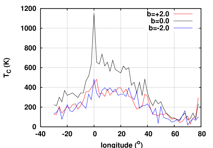
Figure 2: Continuum temperature measured towards all the directions, $-32^{o}<l<+80^{o}$ and $b<\pm 3^{o}$ at 328 MHz and $2^{o}$ resolution. The measured temperatures in the Galactic plane(b=0.0) are in very good agreement with earlier observations(Roshi & Anantharamaiah 2000).

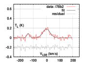
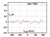
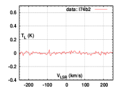
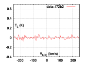
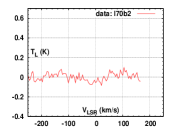
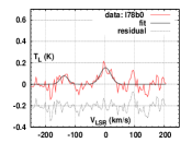
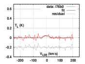
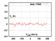
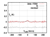
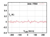
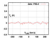
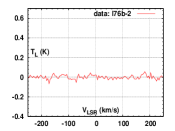
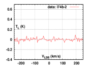
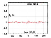
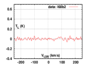
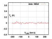
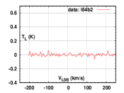
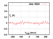
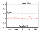
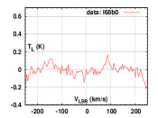
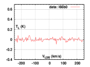
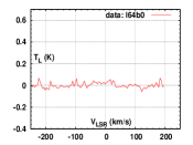
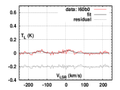
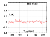
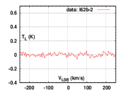
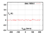
Figure 3: ORT H271$\alpha$ RL observation.

The final calibrated spectra obtained towards all the positions in the Galactic region $-32^{o}<l<+80^{o}$ and $b<\pm 3^{o}$ have been displayed in Figure 3 to 8. The gaussian parameters fitted to these spectra have been given in Table 1.

4 Distribution of ELDWIM in the inner Galaxy

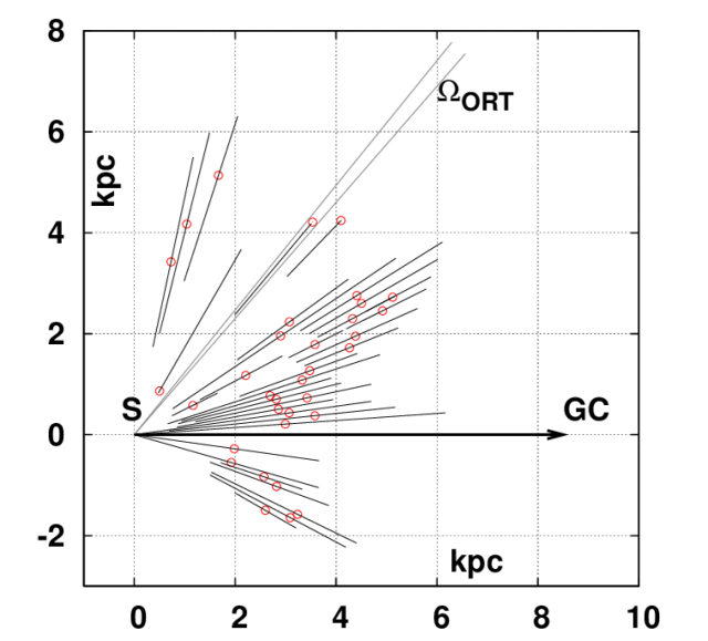
Figure 9: Distribution of ELDWIM clouds in the plane(b=$0^{o}$) of the Galaxy. The origin marks the Solar system S and GC is the Galactic Center. $\Omega_{ORT}$ is the beam of ORT. The red circles mark the center of line origin obtained from the fitted $V_{LSR}$. The length of the line through these circles is the FWHM converted to distance, indicating an upper limit on the spread of the gas. Due to observed $V_{LSR}$ the clouds above(b=+$2^{o}$) and below(b=-$2^{o}$) the plane follow a similar distribution.

Kinematical distances to ELDWIM clouds were obtained from a Galactic rotation curve(Sofue et al. 2009) using the $V_{LSR}$ of H271$\alpha$ RLs. Distribution of these clouds in the plane(b=$0^{o}$) of the Galaxy has been shown in Figure 9. Due to observed $V_{LSR}$ of clouds above and below the plane there is a similar distribution in these regions as well. The width of the lines indicates an upper limit on the spread of gas along the line of sight. The FWHM of the hydrogen lines mostly lie within 20-60 km$s^{-1}$. The profiles also seem to lack pressure broadening(Brocklehurst & Leeman 1971; Shaver 1975) due to absence of extended wings. All the profiles are compatible with a gaussian fit. From this, one can deduce that the number density of electrons $n_{e}$ to have an upper cutoff of 10$cm^{-3}$(Baddi 2011b; Baddi 2012) in ELDWIM. At this density and frequency the pressure broadening contribution is $\sim$ 10 km$s^{-1}$. The average error on the hydrogen line widths is contained within this.

5 Acknowledgement

The author thanks T.Prabu and D.Anish Roshi who helped in doing the observations by providing the new system for spectral line observations, related software and suggestions. The author thanks the staff of Radio Astronomy Center TIFR who have made these observations possible. Ooty Radio Telescope is operated by National Center for Radio Astrophysics TIFR.

The author thanks the refree for suggestions and comments that improved the presentation of the paper.

Table 1: Gaussian parameters for profiles in Figure 3 to 8, the values in the paranthesis are errors. Comments: C-carbon line, H-hydrogen line, ND-no data, NLD-no line detection. $D_{c}$ flags : $f$-far, $n$-near, $m$-distance for maximum $V_{LSR}$ possible from rotation curve. Positions with errors in $V_{LSR}$ greater than 50% have been provided with an upper limit between bars taking into account the full value of errors, especially near $l=0^{o}$.

Source				$T_{L}$			$V_{LSR}$			$\Delta V_{LSR}$			$T_{c}$			$D_{c}$			Comments
$l^{o}$	$b^{o}$			(mK)			(km$s^{-1}$)			(km$s^{-1}$)			(K)			kpc
78	+2			83(20)			-138(3)			26(7)			297						C
				182(13)			0(2)			64(5)						$3.7^{f}$			H
78	0			78(34)			-137(7)			31(15)			234						C
				155(29)			2(4)			42(9)						$3.5^{f}$			H
78	-2			-			-			-			104						H
76	+2			-			-			-			104						NLD
76	0			45(12)			0(6)			44(13)			78			$4.3^{f}$			H
76	-2			-			-			-			66						NLD
74	+2			-			-			-			91						NLD
74	0			-			-			-			140						NLD
74	-2			-			-			-			84						NLD
72	+2			-			-			-			28						NLD
72	0			40(10)			0(4)			32(9)			84			$5.4^{f}$			H?
72	-2			-			-			-			55						NLD
70	+2			-			-			-			-						ND
70	0			-			-			-			72						NLD
70	-2			-			-			-			18						NLD
68	+2			-			-			-			91						NLD
68	0			-			-			-			140						NLD
68	-2			-			-			-			163						NLD
66	+2			-			-			-			55						NLD
66	0			-			-			-			111						NLD
66	-2			-			-			-			111						NLD
64	+2			-			-			-			44						NLD
64	0			-			-			-			72						NLD
64	-2			-			-			-			60						NLD
62	+2			-			-			-			78						NLD
62	0			-			-			-			72						NLD
62	-2			-			-			-			72						NLD
60	+2			-			-			-			84						NLD
60	0			32(8)			-135(5)			40(11)			91						C
				37(7)			16(5)			56(12)						$1.0^{n}$			H
60	-2			-			-			-			55						NLD
58	+2			-			-			-			78						NLD
58	0			-			-			-			91						ND
58	-2			-			-			-			49						NLD
56	+2			-			-			-			104						NLD
56	0			-			-			-			118						ND
56	-2			-			-			-			78						NLD
54	+2			-			-			-			140						NLD
54	0			-			-			-			140						ND
54	-2			-			-			-			84						NLD
52	+2			-			-			-			125						NLD
52	0			-			-			-			188						ND
52	-2			-			-			-			97						NLD
50	+2			-			-			-			132						NLD
50	0			108(18)			68(3)			41(8)			254			$5.5^{m}$			H
50	-2			-			-			-			206						NLD
48	+2			-			-			-			111						NLD
48	0			-			-			-			234						NLD
48	-2			-			-			-			38						NLD
46	+2			-			-			-			125						NLD
46	0			112(26)			78(3)			28(7)			275			$5.9^{m}$			H
46	-2			-			-			-			188						NLD
44	+2			-			-			-			125						NLD
44	0			-			-			-			215						NLD
44	-2			-			-			-			132						NLD
42	+2			-			-			-			197						NLD
42	0			-			-			-			265						NLD
42	-2			-			-			-			188						NLD
40	+2			-			-			-			308						NLD
40	0			-			-			-			344						NLD
40	-2			-			-			-			234						NLD
38	+2			126(22)			-132(3)			34(7)			332						C
				106(28)			36(3)			21(6)						$2.0^{n}$			H
38	0			-			-			-			482						NLD
38	-2			-			-			-			215						NLD
36	+2			75(15)			-132(4)			40(10)			206						C
				78(17)			95(4)			33(8)						$6.2^{n}$			H
36	0			69(12)			-107(6)			66(13)			320						C
				119(15)			65(3)			42(6)						$3.8^{n}$			H
36	-2			-			-			-			215						NLD
34	+2			-			-			-			197						NLD
34	0			153(22)			-121(4)			58(9)			452						C
				131(18)			59(6)			84(13)						$3.5^{n}$			H
34	-2			-			-			-			188						NLD
32	+2			92(15)			89(2)			27(5)			180			$5.1^{n}$			H
32	0			213(18)			90(2)			48(5)			344			$5.2^{n}$			H
32	-2			150(50)			83(4)			25(10)			357			$4.8^{n}$			H
30	+2			38(11)			81(7)			46(15)			234			$4.7^{n}$			H
30	0			325(35)			91(2)			46(6)			452			$5.2^{n}$			H
30	-2			68(17)			87(4)			32(9)			357			$5.0^{n}$			H
28	+2			111(26)			83(4)			35(9)			297			$4.8^{n}$			H
28	0			296(28)			39(-)			30(-)			423			$2.5^{n}$			H
				543(33)			87(-)			35(-)						$4.9^{n}$			H
				92(40)			104(-)			23(-)						$5.8^{n}$			H
28	-2			65(17)			90(5)			37(11)			308			$5.1^{n}$			H
26	+2			161(37)			86(3)			30(8)			308			$2.0^{n}$			H
26.5	0			92(26)			-70(4)			30(10)			500						C
				50(30)			21(-)			15(-)						$1.3^{n}$			H
				166(24)			67(-)			25(-)						$4.0^{n}$			H
				349(21)			98(-)			33(-)						$5.5^{n}$			H
26	-2			113(21)			86(4)			43(9)			396			$4.9^{n}$			H
24	+2			122(22)			87(4)			41(9)			382			$5.0^{n}$			H
24	0			97(23)			-105(9)			73(21)			582						C?
				262(27)			82(3)			56(7)						$4.8^{n}$			H
24	-2			75(17)			86(4)			39(10)			308			$5.0^{n}$			H
22	+2			132(25)			65(5)			56(12)			344			$4.2^{n}$			H
22	0			180(35)			76(4)			45(10)			618			$4.6^{n}$			H
22	-2			-			-			-			332						NLD
20	+2			147(37)			26(3)			27(8)			396			$2.1^{n}$			H
20	0			113(52)			-115(4)			17(10)			547						C
				188(32)			51(4)			46(9)						$3.7^{n}$			H
20	-2			43(22)			-138(7)			26(16)			332						C
				87(14)			60(5)			70(13)						$4.1^{n}$			H
18	+2			72(17)			-128(10)			84(23)			396						C
				227(27)			28(2)			33(5)						$2.4^{n}$			H
18	0			110(33)			-115(10)			69(24)			564						C
				282(32)			44(4)			71(9)						$3.5^{n}$			H
18	-2			66(14)			47(8)			77(19)			320			$3.6^{n}$			H
16	+2			102(22)			-132(4)			40(10)			357						C
				179(23)			29(2)			34(5)						$2.7^{n}$			H
16	0			162(29)			-128(3)			35(7)			582						C
				337(26)			31(2)			41(4)						$2.8^{n}$			H
16	-2			177(31)			-151(2)			29(6)			382						C
				121(26)			32(4)			41(10)						$2.9^{n}$			H
14	+2			108(26)			29(4)			34(9)			357			$2.9^{n}$			H
14	0			243(27)			-122(2)			42(5)			676						C
				448(27)			29(1)			41(3)						$2.9^{n}$			H
14	-2			122(29)			-149(3)			26(7)			357						C
				94(25)			30(5)			36(11)						$3.0^{n}$			H
12	+2			108(23)			-150(2)			21(5)			320						C
				92(19)			21(3)			33(8)						$2.5^{n}$			H
12	0			178(28)			-126(4)			47(9)			564						C
				354(29)			32(2)			44(4)						$3.5^{n}$			H
12	-2			53(20)			-146(11)			58(25)			396						C
				127(24)			25(4)			40(9)						$2.9^{n}$			H
10	+2			69(42)			-142(6)			18(13)			382						C
				102(34)			20(5)			28(11)						$2.8^{n}$			H
10	0			172(26)			-126(3)			43(8)			656						C
				381(26)			21(1)			44(3)						$2.9^{n}$			H
10	-2			65(21)			-143(8)			49(18)			369						C
				192(25)			23(2)			33(5)						$3.1^{n}$			H
8	+2			80(33)			17(4)			21(10)			308			$2.9^{n}$			H
8	0			148(19)			-139(4)			63(9)			618						C
				328(25)			19(1)			36(3)						$3.1^{n}$			H
8	-2			85(36)			-142(4)			20(10)			396						C
				153(33)			17(2)			23(6)						$2.9^{n}$			H
6	+2			44(49)			-134(9)			16(21)			344						C
				70(49)			11(6)			16(13)						$2.6^{n}$			H
6	0			268(39)			-145(4)			58(10)			738						C
				441(53)			18(2)			31(4)						$3.6^{n}$			H
6	-2			105(24)			-148(5)			48(13)			369						C
				156(35)			14(2)			23(6)						$3.1^{n}$			H
4	+2			112(33)			9(4)			30(10)			332			3.0			H
4	0			164(34)			-141(4)			37(9)			637						C
				240(39)			9(2)			29(5)						$3.0^{n}$			H
4	-2			68(28)			-145(3)			16(8)			297						C
				97(27)			15(2)			18(6)						$4.1^{n}$			H
2	+2			-			-			-			482						NLD
2	0			223(52)			-151(2)			22(6)			656						C
				270(51)			0(2)			22(5)						$|1.5|^{n}$			H
2	-2			94(23)			20(6)			48(13)			344			$6.2^{n}$			H
0	+2			79(28)			-142(7)			42(17)			437						C
				197(33)			12(3)			31(6)						-			H
0	0			345(74)			-149(2)			20(5)			1150						C
				680(149)			0(2)			24(5)						-			H
				140(57)			33(22)			42(42)						-			H
0	-2			122(25)			-145(5)			53(13)			482						C
				148(30)			5(4)			37(9)						-			H
-2	+2			57(42)			-3(7)			18(15)			396			$2.0^{n}$			H
-2	0			189(47)			-155(4)			29(8)			656						C
				259			0(3)			37(7)						$|2|^{n}$			H
-2	-2			94(24)			-158(3)			25(7)			275						C
				114(20)			0(3)			35(7)						$|2|^{n}$			H
-4	+2			147(60)			0(6)			29(14)			357			$|1.8|^{n}$			H
-4	0			188(42)			-153(3)			24(6)			514						C
				233(33)			0(3)			37(6)						$|1.0|^{n}$			H
-4	-2			90(28)			-154(3)			22(8)			332						C
				129(27)			0(2)			24(6)						$|1.0|^{n}$			H
-6	+2			71(30)			-121(7)			36(17)			357						C
				169(24)			0(4)			54(9)						$|1.0|^{n}$			H
-6	0			71(36)			-158(9)			36(21)			467						C
				203(44)			0(3)			24(6)						$|1.0|^{n}$			H
-6	-2			100(13)			0(5)			72(11)			188			$|1.2|^{n}$			H
-8	+2			147(55)			0(7)			36(15)			265			$|1.4|^{n}$			H
-8	0			69(29)			-159(4)			20(10)			344						C
				183(22)			-9(2)			33(5)						$2.0^{n}$			H
-8	-2			72(23)			-119(6)			41(15)			215						C?
				109(20)			-11(5)			51(11)						$2.0^{n}$			H
-10	+2			137(46)			-10(6)			35(14)			215			$|2.3|^{n}$			H
-10	0			106(36)			-15(5)			27(11)			344			$2.3^{n}$			H
-10	-2			131(36)			-10(5)			37(12)			254			$|2.3|^{n}$			H
-12	+2			79(15)			-13(5)			51(11)			180			$1.7^{n}$			H
-12	0			-			-			-			297						NLD
-12	-2			101(62)			-24(19)			64(45)			234			$|4.2|^{n}$			H?
-14	+2			113(43)			-8(5)			29(13)			234			$|1.6|^{n}$			H
-14	0			135(21)			-17(4)			49(9)			320			$|2.0|^{n}$			H
-14	-2			-			-			-			188						NLD
-16	+2			125(43)			-17(8)			45(18)			224			$1.7^{n}$			H
-16	0			154(29)			-20(5)			49(11)			344			$2.0^{n}$			H
-16	-2			-			-			-			155						NLD
-18	+2			104(35)			-10(5)			32(12)			188			$|1.3|^{n}$			H
-18	0			135(45)			-154(2)			12(4)			332						C?
				113(31)			-33(3)			24(8)						$2.7^{n}$			H
-18	-2			-			-			-			163						ND
-20	+2			-			-			-			206						NLD
-20	0			78(33)			-40(9)			41(21)			320			$3.0^{n}$			H
-20	-2			-			-			-			224						NLD
-22	+2			-			-			-			171						ND
-22	0			-			-			-			369						NLD
-22	-2			50(11)			-29(5)			46(11)			155			$2.1^{n}$			H
-24	+2			-			-			-			140						NLD
-24	0			-			-			-			254						NLD
-24	-2			25(7)			-33(6)			44(15)			78			$2.3^{n}$			H?
-26	+2			-			-			-			207						NLD
-26	0			175(45)			-56(7)			59(17)			301			$3.6^{n}$			H
-26	-2			112(95)			-60(16)			32(39)			191			$3.8^{n}$			H
				78(95)			-11(22)			33(56)						$2.2^{n}$			H
-28	+2			-			-			-			125						NLD
-28	0			108(29)			-55(7)			56(17)			215			$3.5^{n}$			H
-28	-2			90(33)			-77(5)			30(13)			147			$4.6^{n}$			H
-30	+2			-			-			-			125						NLD
-30	0			139(28)			-50(2)			23(5)			225			$3.0^{n}$			H
-30	-2			-			-			-			132						NLD

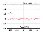
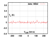
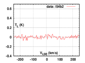
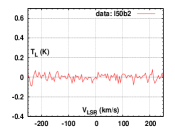
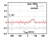
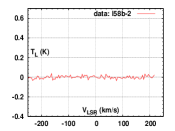
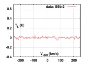
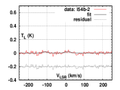
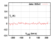
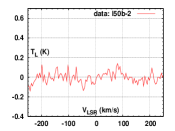
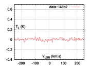
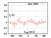
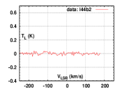
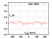
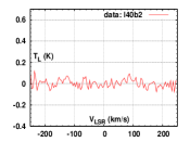
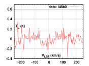
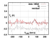
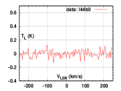
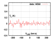
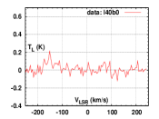
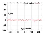
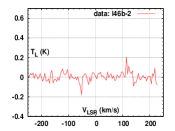
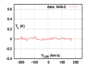
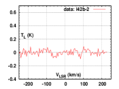
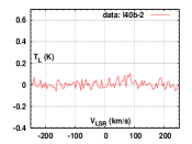
Figure 4: ORT H271$\alpha$ RL observation.

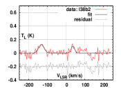
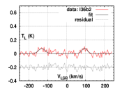
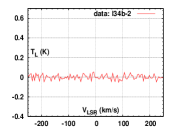
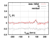
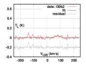
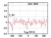
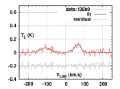
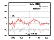
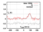
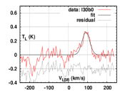
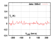
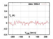
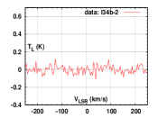
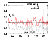
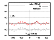
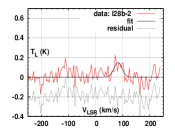
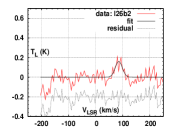
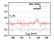
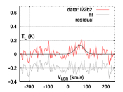
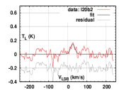
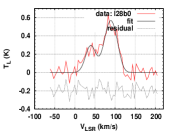
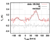
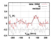
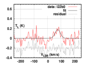
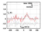
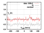
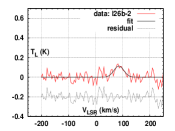
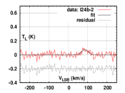
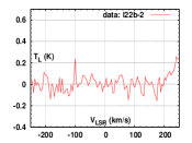
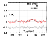
Figure 5: ORT H271$\alpha$ RL observation.

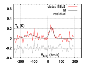
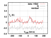
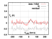
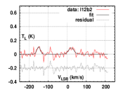
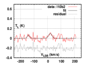
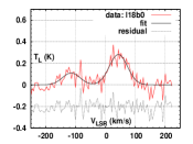
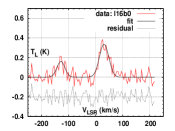
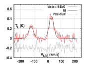
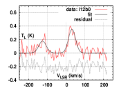
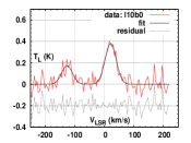
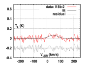
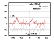
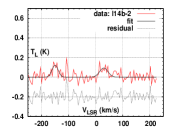
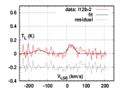
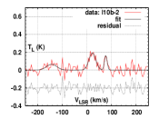
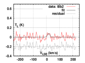
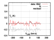
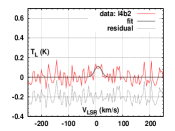
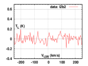
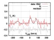
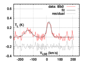
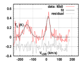
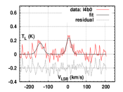
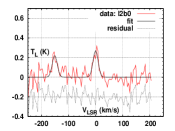
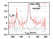
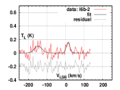
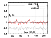
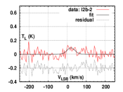
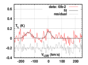
Figure 6: ORT H271$\alpha$ RL observation.

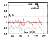
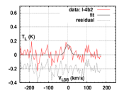
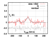
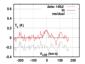
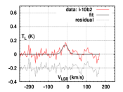
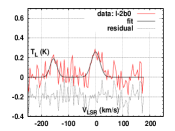
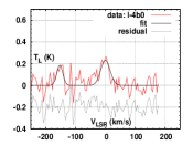
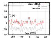
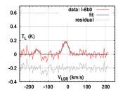
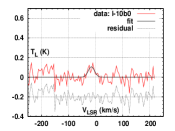
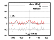
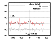
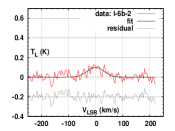
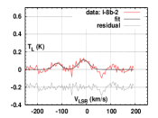
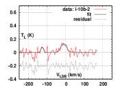
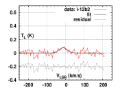
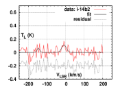
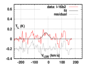
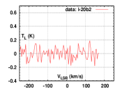
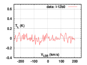
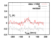
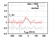
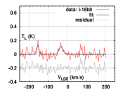
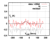
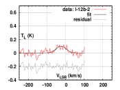
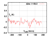
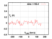
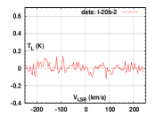
Figure 7: ORT H271$\alpha$ RL observation.

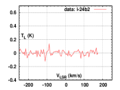
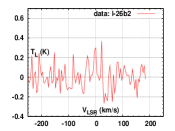
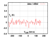
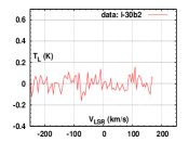
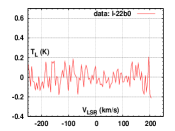
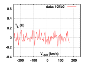
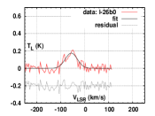
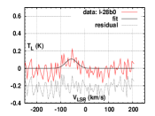
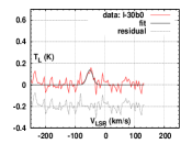
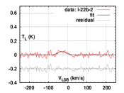
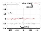
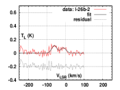
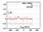
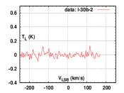
Figure 8: ORT H271$\alpha$ RL observation.

References

- (1) Anantharamaiah, K. R., Journal of Astrophysics and Astronomy, 1985JApA….6..177A
- (2) Anantharamaiah, K. R., Journal of Astrophysics and Astronomy, 1985JApA….6..203A
- (3) Anantharamaiah, K. R., Journal of Astrophysics and Astronomy, 1986JApA….7..131A
- (4) Baddi, R., 2011a, Astronmical Journal, 141, 190B .
- (5) Baddi, R., 2011b, Astronmical Journal, 141, 154B .
- (6) Baddi, R., 2012, Astronmical Journal, in preparation, submitted aug24-2011 .
- (7) Batty, M.J. 1976, Aust. J. Phys., 29, 419 .
- (8) Brocklehurst, M., Leeman, S. 1971, Astrophys. Lett., 9, 35 .
- (9) Dravskikh, A.F., Dravskikh, Z.V., Kolbasov, V.A., Misezhnikov, G.S., Nikulin, D.E. and Shteinshleiger, V.B., 1965, Dok. Akad. Nauk SSSR 163, 332. English translation: 1996, Sov. Phys. - Dokl. 10, 627 .
- (10) Egorova, T.M. and Ryzkov, N.F., 1960, Izv. Glavn. Astrofiz. Obs. 21, 140 .
- (11) Goldberg, L. and Dupree, A.K., 1967, Nature 215, 41 .
- (12) Gottesman, S.T., Gordon, M.A. 1970, Astrophys. J., 162, L93 .
- (13) Lilley, A.E., Palmer, P., Penfield, H. and Zuckerman, B., 1966, Nature 211, 174 .
- (14) Prabu T., 2010, A New Digital Receiver for the Ooty Radio Telescope , Ph.D Thesis submitted to INDIAN INSTITUTE OF SCIENCE, Bangalore-12, India .
- (15) Roshi, D. Anish, Anantharamaiah, K. R., 2000 ApJ…557..226R
- (16) Roshi, D. Anish, Anantharamaiah, K. R., 2001a JApA…22..81
- (17) Roshi, D. Anish, Anantharamaiah, K. R., 2001b ApJ…557..226R
- (18) Shaver, P.A., 1975, Pramana 5, 1 .
- (19) Sofue, Y., Honma, M. and Omodaka, T.2009, PASJ, 61, 227 .
- (20) Swarup, G., et al 1971, Nature, Phys. Science (Lond), 230, 185 .