A generalized mean-reverting equation and applications

Abstract.

Consider a mean-reverting equation, generalized in the sense it is driven by a $1$-dimensional centered Gaussian process with Hölder continuous paths on $[0,T]$ ($T>0$). Taking that equation in rough paths sense only gives local existence of the solution because the non-explosion condition is not satisfied in general. Under natural assumptions, by using specific methods, we show the global existence and uniqueness of the solution, its integrability, the continuity and differentiability of the associated Itô map, and we provide an $L^{p}$-converging approximation with a rate of convergence ($p\geqslant 1$). The regularity of the Itô map ensures a large deviation principle, and the existence of a density with respect to Lebesgue’s measure, for the solution of that generalized mean-reverting equation. Finally, we study a generalized mean-reverting pharmacokinetic model.

MSC2010 : 60H10.

Acknowledgements. Many thanks to my Ph.D. supervisor Laure Coutin for her precious help and advices. This work was supported by A.N.R. Masterie.

1. Introduction

Let $W$ be a $1$-dimensional centered Gaussian process with $\alpha$-Hölder continuous paths on $[0,T]$ ($T>0$ and $\alpha\in]0,1]$).

Consider the stochastic differential equation (SDE) :

(1) $$X_{t}=x_{0}+\int_{0}^{t}\left(a-bX_{u}\right)du+\sigma\int_{0}^{t}X_{u}^{\beta}dW_{u}\textrm{ ; }t\in[0,T]$$

where, $x_{0}>0$ is a deterministic initial condition, $a,b,\sigma\geqslant 0$ are deterministic constants and $\beta$ satisfies the following assumption :

Assumption 1.1.

The exponent $\beta$ satisfies : $\beta\in]1-\alpha,1]$.

When the driving signal is a standard Brownian motion, equation (1) taken in the sense of Itô, is used in many applications. For example, it is studied and applied in finance by J-P. Fouque et al. in [6] for $\beta\in[1/2,1[$. The cornerstone of their approach is the Markov property of diffusion processes. In particular, their proof of the global existence and uniqueness of the solution at Appendix A involves S. Karlin and H.M. Taylor [10], Lemma 6.1(ii). Still for $\beta\in[1/2,1[$, the convergence of the Euler approximation is proved by X. Mao et al. in [17] and [25]. For $\beta\geqslant 1$, equation (1) is studied by F. Wu et al. in [25]. Recently, in [21], N. Tien Dung got an expression and shown the Malliavin’s differentiability of a class of fractional geometric mean-reverting processes.

Equation (1) is a generalization of the mean-reverting equation. In this paper, we study various properties of (1) by taking it in the sense of rough paths (cf. T. Lyons and Z. Qian [14]). Note that Doss-Sussman’s method could also be used since (1) is a $1$-dimensional equation (cf. H. Doss [5] and H.J. Sussman [24]). A priori, even in these senses, equation (1) admits only a local solution because it doesn’t satisfy the non-explosion condition of [8], Exercice 10.56.

At Section 2, we state useful results on rough differential equations (RDEs) and Gaussian rough paths coming from P. Friz and N. Victoir [8]. Section 3 is devoted to study deterministic properties of (1). We show existence and uniqueness of the solution for equation (1), provide an explicit upper-bound for that solution and study the continuity and differentiability of the associated Itô map. We also provide a converging approximation with a rate of convergence. Section 4 is devoted to study probabilistic properties of (1) ; properties of the solution’s distribution, various integrability results, a large deviation principle and the existence of a density with respect to Lebesgue’s measure on $(\mathbb{R},\mathcal{B}(\mathbb{R}))$ for the solution of (1). Finally, at Section 5, we study a pharmacokinetic model based on a particular generalized mean-reverting (M-R) equation (inspired by K. Kalogeropoulos et al. [11]).

2. Rough differential equations and Gaussian rough paths

Essentially inspired by P. Friz and N. Victoir [8], this section provides useful definitions and results on RDEs and Gaussian rough paths.

In a sake of completeness, results on rough differential equations are stated in the multidimensional case.

In the sequel, $\|.\|$ denotes the euclidean norm on $\mathbb{R}^{d}$ and $\|.\|_{\mathcal{M}}$ the usual norm on $\mathcal{M}_{d}(\mathbb{R})$ $(d\in\mathbb{N}^{*})$.

Consider $D_{T}$ the set of subdivisions for $[0,T]$ and

$$\Delta_{T}=\left\{(s,t)\in\mathbb{R}_{+}^{2}:0\leqslant s<t\leqslant T\right\}.$$

Let $T^{N}(\mathbb{R}^{d})$ be the step-$N$ tensor algebra over $\mathbb{R}^{d}$ ($N\in\mathbb{N}^{*}$) :

$$T^{N}\left(\mathbb{R}^{d}\right)=\bigoplus_{i=0}^{N}\left(\mathbb{R}^{d}\right)^{\otimes i}.$$

For $i=1,\dots,N$, $(\mathbb{R}^{d})^{\otimes i}$ is equipped with its euclidean norm $\|.\|_{i}$, $(\mathbb{R}^{d})^{\otimes 0}=\mathbb{R}$ and the canonical projection on $(\mathbb{R}^{d})^{\otimes i}$ for any $Y\in T^{N}(\mathbb{R}^{d})$ is denoted by $Y^{i}$.

First, let’s remind definitions of $p$-variation and $\alpha$-Hölder norms ($p\geqslant 1$ and $\alpha\in[0,1]$) :

Definition 2.1.

Consider $y:[0,T]\rightarrow\mathbb{R}^{d}$ :

1. The function $y$ has finite $p$-variation if and only if,

   $$\|y\|_{p\textrm{-var};T}=\sup_{D=\{r_{k}\}\in D_{T}}\left(\sum_{k=1}^{|D|-1}\|y_{r_{k+1}}-y_{r_{k}}\|^{p}\right)^{1/p}<\infty.$$

2. The function $y$ is $\alpha$-Hölder continuous if and only if,

   $$\|y\|_{\alpha\textrm{-H\"{o}l};T}=\sup_{(s,t)\in\Delta_{T}}\frac{\|y_{t}-y_{s}\|}{|t-s|^{\alpha}}<\infty.$$

In the sequel, the space of continuous functions with finite $p$-variation will be denoted by :

$$C^{p\textrm{-var}}\left([0,T];\mathbb{R}^{d}\right).$$

The space of $\alpha$-Hölder continuous functions will be denoted by :

$$C^{\alpha\textrm{-H\"{o}l}}\left([0,T];\mathbb{R}^{d}\right).$$

If it is not specified, these spaces will always be equipped with norms $\|.\|_{p\textrm{-var};T}$ and $\|.\|_{\alpha\textrm{-H\"{o}l};T}$ respectively.

Remark. Note that :

$$C^{\alpha\textrm{-H\"{o}l}}\left([0,T];\mathbb{R}^{d}\right)\subset C^{1/\alpha\textrm{-var}}\left([0,T];\mathbb{R}^{d}\right).$$

Definition 2.2.

Let $y:[0,T]\rightarrow\mathbb{R}^{d}$ be a continuous function of finite $1$-variation. The step-$N$ signature of $y$ is the functional $S_{N}(y):\Delta_{T}\rightarrow T^{N}(\mathbb{R}^{d})$ such that for every $(s,t)\in\Delta_{T}$ and $i=1,\dots,N$,

$$S_{N;s,t}^{0}(y)=1\textrm{ and }S_{N;s,t}^{i}(y)=\int_{s<r_{1}<r_{2}<\dots<r_{i}<t}dy_{r_{1}}\otimes\dots\otimes dy_{r_{i}}.$$

Moreover,

$$G^{N}(\mathbb{R}^{d})=\left\{S_{N;0,T}(y);y\in C^{1\textrm{-var}}([0,T];\mathbb{R}^{d})\right\}$$

is the step-$N$ free nilpotent group over $\mathbb{R}^{d}$.

Definition 2.3.

A map $Y:\Delta_{T}\rightarrow G^{N}(\mathbb{R}^{d})$ is of finite $p$-variation if and only if,

$$\|Y\|_{p\textrm{-var};T}=\sup_{D=\left\{r_{k}\right\}\in D_{T}}\left(\sum_{k=1}^{|D|-1}\|Y_{r_{k},r_{k+1}}\|_{\mathcal{C}}^{p}\right)^{1/p}<\infty$$

where, $\|.\|_{\mathcal{C}}$ is the Carnot-Caratheodory’s norm such that for every $g\in G^{N}(\mathbb{R}^{d})$,

$$\|g\|_{\mathcal{C}}=\inf\left\{\mathbf{length}(y);y\in C^{1\textrm{-var}}([0,T];\mathbb{R}^{d})\textrm{ and }S_{N;0,T}(y)=g\right\}.$$

In the sequel, the space of continuous functions from $\Delta_{T}$ into $G^{N}(\mathbb{R}^{d})$ with finite $p$-variation will be denoted by :

$$C^{p\textrm{-var}}([0,T];G^{N}(\mathbb{R}^{d})).$$

If it is not specified, that space will always be equipped with $\|.\|_{p\textrm{-var};T}$.

Let’s define the Lipschitz regularity in the sense of Stein :

Definition 2.4.

Consider $\gamma>0$. A map $V:\mathbb{R}^{d}\rightarrow\mathbb{R}$ is $\gamma$-Lipschitz (in the sense of Stein) if and only if $V$ is $C^{\lfloor\gamma\rfloor}$ on $\mathbb{R}^{d}$, bounded, with bounded derivatives and such that the $\lfloor\gamma\rfloor$-th derivative of $V$ is $\{\gamma\}$-Hölder continuous ($\lfloor\gamma\rfloor$ is the largest integer strictly smaller than $\gamma$ and $\{\gamma\}=\gamma-\lfloor\gamma\rfloor$).

The least bound is denoted by $\|V\|_{\textrm{lip}^{\gamma}}$. The map $\|.\|_{\textrm{lip}^{\gamma}}$ is a norm on the vector space of collections of $\gamma$-Lipschitz vector fields on $\mathbb{R}^{d}$, denoted by $\textrm{Lip}^{\gamma}(\mathbb{R}^{d})$.

In the sequel, $\textrm{Lip}^{\gamma}(\mathbb{R}^{d})$ will always be equipped with $\|.\|_{\textrm{lip}^{\gamma}}$.

Let $w:[0,T]\rightarrow\mathbb{R}^{d}$ be a continuous function of finite $p$-variation such that a geometric $p$-rough path $\mathbb{W}$ exists over it. In other words, there exists an approximating sequence $(w^{n},n\in\mathbb{N})$ of functions of finite $1$-variation such that :

$$\lim_{n\rightarrow\infty}d_{p\textrm{-var};T}\left[S_{[p]}\left(w^{n}\right);\mathbb{W}\right]=0.$$

When $d=1$, a natural geometric $p$-rough path $\mathbb{W}$ over it is defined by :

(2) $$\forall(s,t)\in\Delta_{T}\textrm{, }\mathbb{W}_{s,t}=\left(1,w_{t}-w_{s},\dots,\frac{(w_{t}-w_{s})^{[p]}}{[p]!}\right).$$

We remind that if $V=(V_{1},\dots,V_{d})$ is a collection of Lipschitz continuous vector fields on $\mathbb{R}^{d}$, the ordinary differential equation $dy=V(y)dw^{n}$, with initial condition $y_{0}\in\mathbb{R}^{d}$, admits a unique solution.

That solution is denoted by $\pi_{V}(0,y_{0};w^{n})$.

Rigorously, a RDE’s solution is defined as follow (cf. [8], Definition 10.17) :

Definition 2.5.

A continuous function $y:[0,T]\rightarrow\mathbb{R}^{d}$ is a solution of $dy=V(y)d\mathbb{W}$ with initial condition $y_{0}\in\mathbb{R}^{d}$ if and only if,

$$\lim_{n\rightarrow\infty}\left\|\pi_{V}(0,y_{0};w^{n})-y\right\|_{\infty;T}=0$$

where, $\|.\|_{\infty;T}$ is the uniform norm on $[0,T]$. If there exists a unique solution, it is denoted by $\pi_{V}(0,y_{0};\mathbb{W})$.

Theorem 2.6.

Let $V=(V_{1},\dots,V_{d})$ be a collection of locally $\gamma$-Lipschitz vector fields on $\mathbb{R}^{d}$ ($\gamma>p$) such that : $V$ and $D^{[p]}V$ are respectively globally Lipschitz continuous and $(\gamma-[p])$-Hölder continuous on $\mathbb{R}^{d}$. With initial condition $y_{0}\in\mathbb{R}^{d}$, equation $dy=V(y)d\mathbb{W}$ admits a unique solution $\pi_{V}(0,y_{0};\mathbb{W})$.

For a proof, see P. Friz and N. Victoir [8], Exercice 10.56.

For P. Friz and N. Victoir, the rough integral for a collection of $(\gamma-1)$-Lipschitz vector fields $V=(V_{1},\dots,V_{d})$ along $\mathbb{W}$ is the projection of a particular full RDE’s solution (cf. [8], Definition 10.34 for full RDEs) : $d\mathbb{X}=\Phi(\mathbb{X})d\mathbb{W}$ where,

$$\forall i=1,\dots,d\textrm{, }\forall a,w\in\mathbb{R}^{d}\textrm{, }\Phi_{i}(w,a)=(e_{i},V_{i}(w))$$

and $(e_{1},\dots,e_{d})$ is the canonical basis of $\mathbb{R}^{d}$.

In particular, if $y:[0,T]\rightarrow\mathcal{M}_{d}(\mathbb{R})$ and $z:[0,T]\rightarrow\mathbb{R}^{d}$ are two continuous functions, respectively of finite $p$-variation and finite $q$-variation with $1/p+1/q>1$, the Young integral of $y$ with respect to $z$ is denoted by $\mathcal{Y}(y,z)$.

Remark. We are not developing the notion of full RDE in that paper because it is not useful in the sequel. As mentioned above, the reader can refer to [8], Definition 10.34 for details.

For a proof of the following change of variable formula for geometric rough paths, cf. [2], Theorem 53 :

Theorem 2.7.

Let $\Phi$ be a collection of $\gamma$-Lipschitz vector fields on $\mathbb{R}^{d}$ ($\gamma>p$) and let $\mathbb{W}$ be a geometric $p$-rough path. Then,

$$\forall(s,t)\in\Delta_{T}\textrm{, }\Phi\left(w_{t}\right)-\Phi\left(w_{s}\right)=\left[\int D\Phi(\mathbb{W})d\mathbb{W}\right]_{s,t}^{1}.$$

Now, let state some results on $1$-dimensional Gaussian rough paths :

Consider a stochastic process $W$ defined on $[0,T]$ and satisfying the following assumption :

Assumption 2.8.

$W$ is a $1$-dimensional centered Gaussian process with $\alpha$-Hölder continuous paths on $[0,T]$ ($\alpha\in]0,1]$).

In the sequel, we work on the probability space $(\Omega,\mathcal{A},\mathbb{P})$ where $\Omega=C^{0}([0,T];\mathbb{R})$, $\mathcal{A}$ is the $\sigma$-algebra generated by cylinder sets and $\mathbb{P}$ is the probability measure induced by $W$ on $(\Omega,\mathcal{A})$.

Remark. Since $W$ is a $1$-dimensional Gaussian process, the natural geometric $1/\alpha$-rough path over it defined by (2) is matching with the enhanced Gaussian process for $W$ provided by P. Friz and N. Victoir at [8], Theorem 15.33 in the multidimensional case.

Finally, Cameron-Martin’s space of $W$ is given by :

$$\mathcal{H}_{W}^{1}=\left\{h\in C^{0}([0,T];\mathbb{R}):\exists Z\in\mathcal{A}_{W}\textrm{ s.t. }\forall t\in[0,T]\textrm{, }h_{t}=\mathbb{E}(W_{t}Z)\right\}$$

with

$$\mathcal{A}_{W}=\overline{\textrm{span}\left\{W_{t};t\in[0,T]\right\}}^{L^{2}}.$$

Let $\langle.,.\rangle_{\mathcal{H}_{W}^{1}}$ be the map defined on $\mathcal{H}_{W}^{1}\times\mathcal{H}_{W}^{1}$ by :

$$\langle h,\tilde{h}\rangle_{\mathcal{H}_{W}^{1}}=\mathbb{E}(Z\tilde{Z})$$

where,

$$\forall t\in[0,T]\textrm{, }h_{t}=\mathbb{E}(W_{t}Z)\textrm{ and }\tilde{h}_{t}=\mathbb{E}(W_{t}\tilde{Z})$$

with $Z,\tilde{Z}\in\mathcal{A}_{W}$.

That map is a scalar product on $\mathcal{H}_{W}^{1}$ and, equipped with it, $\mathcal{H}_{W}^{1}$ is a Hilbert space.

The triplet $(\Omega,\mathcal{H}_{W}^{1},\mathbb{P})$ is called an abstract Wiener space (cf. M. Ledoux [12]).

Proposition 2.9.

For $d=1$, consider a random variable $F:\Omega\rightarrow\mathbb{R}$, continuously $\mathcal{H}_{W}^{1}$-differentiable (i.e. $h\mapsto F(\omega+h)$ is continuously differentiable from $\mathcal{H}_{W}^{1}$ into $\mathbb{R}$, for almost every $\omega\in\Omega$).

If $F$ satisfies Bouleau-Hirsch’s condition (i.e. $|D_{h}F|>0$ a.s. for at least one $h\in\mathcal{H}_{W}^{1}$ such that $h\not=0$, where :

$$(D_{\eta}F)(\omega)=\left.\frac{\partial}{\partial\varepsilon}F(\omega+\varepsilon\eta)\right|_{\varepsilon=0}\textrm{, }\forall\eta\in\mathcal{H}_{W}^{1}),$$

then $F$ admits a density with respect to Lebesgue’s measure on $(\mathbb{R},\mathcal{B}(\mathbb{R}))$.

Remarks :

1. Classically, Bouleau-Hirsch’s condition is not stated that way and involves Malliavin calculus framework. Consider the Malliavin derivative operator $\mathbf{D}$ (cf. D. Nualart [20], Section 1.2), the reproducing kernel Hilbert space $\mathcal{H}_{W}$ of the Gaussian process $W$ (cf. J. Neveu [19]), and the canonical isometry $I$ from $\mathcal{H}_{W}$ into $\mathcal{H}_{W}^{1}$ defined for example at N. Marie [18], Section 3.1. Bouleau-Hirsch’s condition for $d=1$ is $\|\mathbf{D}F\|_{\mathcal{H}}^{2}>0$.
   
   On one hand, by Cauchy-Schwarz’s inequality, it is sufficient to show that there exists $h\in\mathcal{H}_{W}^{1}$ satisfying $h\not=0$ and $|\langle\mathbf{D}F,I^{-1}(h)\rangle_{\mathcal{H}}|>0$. On the other hand, with Malliavin calculus methods, one can easily show that $\langle\mathbf{D}F,I^{-1}(h)\rangle_{\mathcal{H}}=D_{h}F$.

2. About Bouleau-Hirsch’s criterion for $d\geqslant 1$, please refer to [20], Theorem 2.1.2.

3. Deterministic properties of the generalized mean-reverting equation

In this section, we show existence and uniqueness of the solution for equation (1), provide an explicit upper-bound for that solution and, study the continuity and differentiability of the associated Itô map. We also provide a converging approximation for equation (1).

Consider a function $w:[0,T]\rightarrow\mathbb{R}$ satisfying the following assumption :

Assumption 3.1.

The function $w$ is $\alpha$-Hölder continuous ($\alpha\in]0,1]$).

Let $\mathbb{W}$ be the natural geometric $1/\alpha$-rough path over $w$ defined by (2). Then, we put $\mathcal{W}=S_{[1/\alpha]}(\textrm{Id}_{[0,T]}\oplus\mathbb{W})$, which is a geometric $1/\alpha$-rough path over

$$t\in[0,T]\longmapsto\left(t,w_{t}\right)$$

by [8], Theorem 9.26.

Remark. For a rigorous construction of Young pairing, the reader can refer to [8], Section 9.4.

Then, consider the rough differential equation :

(3) $$dx=V(x)d\mathcal{W}\textrm{ with initial condition $x_{0}\in\mathbb{R}$,}$$

where $V$ is the map defined on $\mathbb{R}_{+}$ by :

$$\forall x\in\mathbb{R}_{+}\textrm{, }\forall t,w\in\mathbb{R}\textrm{, }V(x).(t,w)=(a-bx)t+\sigma x^{\beta}w.$$

For technical reasons, we introduce another equation :

(4) $$y_{t}=y_{0}+a(1-\beta)\int_{0}^{t}y_{s}^{-\gamma}e^{bs}ds+\tilde{w}_{t}\textrm{ ; }t\in[0,T]\textrm{, }y_{0}>0$$

where, $\gamma=\frac{\beta}{1-\beta}$ and

$$\tilde{w}_{t}=\int_{0}^{t}\vartheta_{s}dw_{s}\textrm{ with }\vartheta_{t}=\sigma(1-\beta)e^{b(1-\beta)t}$$

for every $t\in[0,T]$. The integral is taken in the sense of Young.

The map $u\in[\varepsilon,\infty[\mapsto u^{-\gamma}$ belongs to $C^{\infty}([\varepsilon,\infty[;\mathbb{R})$ and is bounded with bounded derivatives on $[\varepsilon,\infty[$ for every $\varepsilon>0$. Then, equation (4) admits a unique solution in the sense of Definition 2.5 by applying Theorem 2.6 up to the time

$$\tau_{\varepsilon}^{1}=\inf\left\{t\in[0,T]:y_{t}=\varepsilon\right\}\textrm{ ; }\varepsilon\in]0,y_{0}],$$

by assuming that $\inf(\emptyset)=\infty$.

Consider also the time $\tau_{0}^{1}>0$, such that $\tau_{\varepsilon}^{1}\uparrow\tau_{0}^{1}$ when $\varepsilon\rightarrow 0$.

3.1. Existence and uniqueness of the solution

As mentioned above, Section 2 ensures that equation (4) has, at least locally, a unique solution denoted $y$. At Lemma 3.2, we prove it ensures that equation (3) admits also, at least locally, a unique solution (in the sense of Definition 2.5) denoted $x$. In particular, we show that $x=y^{\gamma+1}e^{-b.}$. At Proposition 3.3, we prove the global existence of $y$ by using the fact it never hits $0$ on $[0,T]$. These results together ensures the existence and uniqueness of $x$ on $[0,T]$.

Lemma 3.2.

Consider $y_{0}>0$ and $a,b\geqslant 0$. Under assumptions 1.1 and 3.1, up to the time $\tau_{\varepsilon}^{1}$ ($\varepsilon\in]0,y_{0}]$), if $y$ is the solution of (4) with initial condition $y_{0}$, then

$$x:t\in\left[0,\tau_{\varepsilon}^{1}\right]\longmapsto x_{t}=y_{t}^{\gamma+1}e^{-bt}$$

is the solution of (3) on $[0,\tau_{\varepsilon}^{1}]$, with initial condition $x_{0}=y_{0}^{\gamma+1}$.

Proof.

Consider the solution $y$ of (4) on $[0,\tau_{\varepsilon}^{1}]$, with initial condition $y_{0}>0$.

The continuous function $z=ye^{-b(1-\beta).}$ takes its values in $[m_{\varepsilon},M_{\varepsilon}]\subset\mathbb{R}_{+}^{*}$ on $[0,\tau_{\varepsilon}^{1}]$.

Since $\gamma>0$, the map $\Phi:u\in[m_{\varepsilon},M_{\varepsilon}]\mapsto u^{\gamma+1}$ is $C^{\infty}$, bounded and with bounded derivatives.

Then, by applying the change of variable formula (Theorem 2.7) to $z$ and to the map $\Phi$ between $0$ and $t\in[0,\tau_{\varepsilon}^{1}]$ :

$$x_{t} = z_{0}^{\gamma+1}+(\gamma+1)\int_{0}^{t}z_{s}^{\gamma}dz_{s}$$

$$= y_{0}^{\gamma+1}+\int_{0}^{t}\left(a-bx_{s}\right)ds+\sigma\int_{0}^{t}y_{s}^{\gamma}e^{-b\beta s}dw_{s}.$$

Since $\gamma=\beta(\gamma+1)$, in the sense of Definition 2.5, $x$ is the solution of (3) on $[0,\tau_{\varepsilon}^{1}]$ with initial condition $x_{0}=y_{0}^{\gamma+1}$. ∎

Proposition 3.3.

Under assumptions 1.1 and 3.1, for $a>0$ and $b\geqslant 0$, with initial condition $x_{0}>0$ ; $\tau_{0}^{1}>T$ and then, equation (3) admits a unique solution $\tilde{\pi}_{V}(0,x_{0};w)$ on $[0,T]$, satisfying :

$$\tilde{\pi}_{V}(0,x_{0};w)=\pi_{V}(0,x_{0};\mathcal{W}).$$

Moreover, since $T>0$ is chosen arbitrarily, that notion of solution extends to $\mathbb{R}_{+}$.

Proof.

Suppose that $\tau_{0}^{1}\leqslant T$, put $y_{0}=x_{0}^{1-\beta}$ and consider the solution $y$ of (4) on $[0,\tau_{\varepsilon}^{1}]$ ($\varepsilon\in]0,y_{0}]$), with initial condition $y_{0}$.

On one hand, note that by definition of $\tau_{\varepsilon}^{1}$ :

$$y_{\tau_{\varepsilon}^{1}}-y_{t} = \varepsilon-y_{t}\textrm{ and}$$

$$y_{\tau_{\varepsilon}^{1}}-y_{t} = a(1-\beta)\int_{t}^{\tau_{\varepsilon}^{1}}y_{s}^{-\gamma}e^{bs}ds+\tilde{w}_{\tau_{\varepsilon}^{1}}-\tilde{w}_{t}$$

for every $t\in[0,\tau_{\varepsilon}^{1}]$. Then, since $\tau_{\varepsilon}^{1}\uparrow\tau_{0}^{1}$ when $\varepsilon\rightarrow 0$ :

(5) $$y_{t}+a(1-\beta)\int_{t}^{\tau_{0}^{1}}y_{s}^{-\gamma}e^{bs}ds=\tilde{w}_{t}-\tilde{w}_{\tau_{0}^{1}}$$

for every $t\in[0,\tau_{0}^{1}[$.

Moreover, since $\tilde{w}$ is the Young integral of $\vartheta\in C^{\infty}([0,T];\mathbb{R}_{+})$ against $w$, and $w$ is $\alpha$-Hölder continuous, $\tilde{w}$ is also $\alpha$-Hölder continuous (cf. [8], Theorem 6.8).

Together, equality (5) and the $\alpha$-Hölder continuity of $\tilde{w}$ imply :

$$-\|\tilde{w}\|_{\alpha\textrm{-H\"{o}l};T}(\tau_{0}^{1}-t)^{\alpha}\leqslant y_{t}+a(1-\beta)\int_{t}^{\tau_{0}^{1}}y_{s}^{-\gamma}e^{bs}ds\leqslant\|\tilde{w}\|_{\alpha\textrm{-H\"{o}l};T}(\tau_{0}^{1}-t)^{\alpha}.$$

On the other hand, the two terms of that sum are positive. Then,

(6) $$y_{t} \leqslant \|\tilde{w}\|_{\alpha\textrm{-H\"{o}l};T}(\tau_{0}^{1}-t)^{\alpha}\textrm{ and}$$

(7) $$a(1-\beta)\int_{t}^{\tau_{0}^{1}}y_{s}^{-\gamma}e^{bs}ds \leqslant \|\tilde{w}\|_{\alpha\textrm{-H\"{o}l};T}(\tau_{0}^{1}-t)^{\alpha}.$$

Since $t\in[0,\tau_{0}^{1}[$ has been chosen arbitrarily, inequality (6) is true for every $s\in[t,\tau_{0}^{1}[$ and implies :

$$y_{s}^{-\gamma}\geqslant\|\tilde{w}\|_{\alpha\textrm{-H\"{o}l};T}^{-\gamma}\left(\tau_{0}^{1}-s\right)^{-\alpha\gamma}.$$

So

(8) $$a(1-\beta)\int_{t}^{\tau_{0}^{1}}y_{s}^{-\gamma}e^{bs}ds \geqslant a(1-\beta)\|\tilde{w}\|_{\alpha\textrm{-H\"{o}l};T}^{-\gamma}\int_{t}^{\tau_{0}^{1}}(\tau_{0}^{1}-s)^{-\alpha\gamma}e^{bs}ds$$

$$\geqslant \frac{a(1-\beta)}{1-\alpha\gamma}\|\tilde{w}\|_{\alpha\textrm{-H\"{o}l};T}^{-\gamma}\left[(\tau_{0}^{1}-t)^{1-\alpha\gamma}-\lim_{s\rightarrow\tau_{0}^{1}}(\tau_{0}^{1}-s)^{1-\alpha\gamma}\right].$$

By inequalities (7) and (8) together :

(9) $$\frac{a(1-\beta)}{1-\alpha\gamma}\left[(\tau_{0}^{1}-t)^{1-\alpha\gamma}-\lim_{s\rightarrow\tau_{0}^{1}}(\tau_{0}^{1}-s)^{1-\alpha\gamma}\right]\leqslant\|\tilde{w}\|_{\alpha\textrm{-H\"{o}l};T}^{\gamma+1}(\tau_{0}^{1}-t)^{\alpha}.$$

If $\beta\geqslant 1/(1+\alpha)>1-\alpha$, then $1-\alpha\gamma\leqslant 0$ and

$$\lim_{s\rightarrow\tau_{0}^{1}}-\frac{1}{1-\alpha\gamma}\left(\tau_{0}^{1}-s\right)^{1-\alpha\gamma}=\infty.$$

If $1/(1+\alpha)>\beta>1-\alpha$, inequality (9) can be rewritten as

$$\frac{a(1-\beta)}{1-\alpha\gamma}(\tau_{0}^{1}-t)^{1-\alpha(\gamma+1)}\leqslant\|\tilde{w}\|_{\alpha\textrm{-H\"{o}l};T}^{\gamma+1},$$

but $1-\alpha(\gamma+1)<0$ and

$$\lim_{t\rightarrow\tau_{0}^{1}}\frac{1}{1-\alpha\gamma}\left(\tau_{0}^{1}-t\right)^{1-\alpha(\gamma+1)}=\infty.$$

Therefore, if $\beta>1-\alpha$, $\tau_{0}^{1}\not\in[0,T]$.

An immediate consequence is that :

$$\bigcup_{\varepsilon\in]0,y_{0}]}[0,\tau_{\varepsilon}^{1}]\cap[0,T]=[0,T].$$

Then, (4) admits a unique solution on $[0,T]$ by putting :

$$y=y^{\varepsilon}\textrm{ on }[0,\tau_{\varepsilon}^{1}]\cap[0,T]$$

where, $y^{\varepsilon}$ denotes the solution of (4) on $[0,\tau_{\varepsilon}^{1}]\cap[0,T]$ for every $\varepsilon\in]0,y_{0}]$.

By Lemma 3.2, equation (3) admits a unique solution $\tilde{\pi}_{V}(0,x_{0};w)$ on $[0,T]$, matching with $y^{\gamma+1}e^{-b.}$.

Finally, since $T>0$ is chosen arbitrarily, for $w:\mathbb{R}_{+}\rightarrow\mathbb{R}$ locally $\alpha$-Hölder continuous, equation (3) admits a unique solution $\tilde{\pi}_{V}(0,x_{0};w)$ on $\mathbb{R}_{+}$ by putting :

$$\tilde{\pi}_{V}(0,x_{0};w)=\tilde{\pi}_{V}(0,x_{0};w_{\left|[0,T]\right.})\textrm{ on $[0,T]$}$$

for every $T>0$. ∎

Remarks and partial extensions :

1. Note that the statement of Lemma 3.2 holds true when $a=0$, and up to the time $\tau_{0}^{1}$, equation (3) has a unique explicit solution :

   $$\forall t\in[0,\tau_{0}^{1}]\textrm{, }x_{t}=\left(x_{0}^{1-\beta}+\tilde{w}_{t}\right)^{\gamma+1}e^{-bt}.$$

   However, in that case, $\tau_{0}^{1}$ can belong to $[0,T]$. Then, $x$ is matching with the solution of equation (3) only locally. It is sufficient for the application in pharmacokinetic provided at Section 5.

2. For every $\alpha\in]0,1[$, equation (4) admits a unique solution $y$ on $[0,T]$ when :

   (10) $$\inf_{s\in[0,T]}\tilde{w}_{s}>-y_{0}.$$

   Indeed, for every $t\in[0,\tau_{0}^{1}]$,

   $$y_{t}-a(1-\beta)\int_{0}^{t}y_{s}^{-\gamma}e^{bs}ds=y_{0}+\tilde{w}_{t}.$$

   Then,

   $$\inf_{s\in[0,\tau_{0}^{1}]}y_{s}-a(1-\beta)\sup_{s\in[0,\tau_{0}^{1}]}\int_{0}^{s}y_{u}^{-\gamma}e^{bu}du\geqslant y_{0}+\inf_{s\in[0,T]}\tilde{w}_{s}.$$

   Since $y$ is continuous from $[0,\tau_{0}^{1}]$ into $\mathbb{R}$ with $y_{0}>0$ :

   $$\sup_{s\in[0,\tau_{0}^{1}]}\int_{0}^{s}y_{u}^{-\gamma}e^{bu}du>0.$$

   Therefore,

   (11) $$y_{t} \geqslant \inf_{s\in[0,\tau_{0}^{1}]}y_{s}$$

   $$\geqslant y_{0}+\inf_{s\in[0,T]}\tilde{w}_{s}>0$$

   by inequality (10). Since the right-hand side of inequality (11) is not depending on $\tau_{0}^{1}$, that hitting time is not belonging to $[0,T]$.
   
   By Lemma 3.2, equation (3) admits also a unique solution on $[0,T]$ when (10) is true.

3. If $\tau_{0}^{1}\in[0,T]$, necessarily :

   $$a(1-\beta)\|\tilde{w}\|_{\alpha\textrm{-H\"{o}l};T}^{-\gamma}\int_{t}^{\tau_{0}^{1}}(\tau_{0}^{1}-s)^{-\alpha\gamma}ds\leqslant\|\tilde{w}\|_{\alpha\textrm{-H\"{o}l};T}(\tau_{0}^{1}-t)^{\alpha}$$

   for every $t\in[0,\tau_{0}^{1}[$.
   
   Then, when $\beta=1-\alpha$, $1-\alpha\gamma=\alpha$ and by [8], Theorem 6.8 :

   $$a \leqslant \|\tilde{w}\|_{\alpha\textrm{-H\"{o}l};T}$$

   $$\leqslant C(\sigma,\alpha,b)\|w\|_{\alpha\textrm{-H\"{o}l};T}^{1/\alpha}$$

   with $C(\sigma,\alpha,b)=(\sigma b\alpha^{2})^{1/\alpha}e^{bT}$.
   
   Therefore, $\tilde{\pi}_{V}(0,x_{0};w)$ is defined on $[0,T]$ when $a>C(\sigma,\alpha,b)\|w\|_{\alpha\textrm{-H\"{o}l};T}^{1/\alpha}$.

3.2. Upper-bound for the solution and regularity of the Itô map

Under assumptions 1.1 and 3.1, we provide an explicit upper-bound for $\|\tilde{\pi}_{V}(0,x_{0};w)\|_{\infty;T}$ and, show continuity and differentiability results for the Itô map :

Proposition 3.4.

Under assumptions 1.1 and 3.1, for $a>0$ and $b\geqslant 0$, with any initial condition $x_{0}>0$,

$$\|\tilde{\pi}_{V}(0,x_{0};w)\|_{\infty;T} \leqslant \left[x_{0}^{1-\beta}+a(1-\beta)e^{bT}x_{0}^{-\beta}T+\right.$$

$$\left.\sigma(b\vee 2)(1-\beta)(1+T)e^{b(1-\beta)T}\|w\|_{\infty;T}\right]^{\gamma+1}.$$

Proof.

Consider $y_{0}=x_{0}^{1-\beta}$, $y$ the solution of (4) with initial condition $y_{0}$ and

$$\tau_{y_{0}}^{2}=\sup\left\{t\in[0,T]:y_{t}\leqslant y_{0}\right\}.$$

On one hand, we consider the two following cases :

1. If $t<\tau_{y_{0}}^{2}$ :

   $$y_{\tau_{y_{0}}^{2}}-y_{t}=a(1-\beta)\int_{t}^{\tau_{y_{0}}^{2}}y_{s}^{-\gamma}e^{bs}ds+\tilde{w}_{\tau_{y_{0}}^{2}}-\tilde{w}_{t}.$$

   Then, by definition of $\tau_{y_{0}}^{2}$ :

   (12) $$y_{t}+a(1-\beta)\int_{t}^{\tau_{y_{0}}^{2}}y_{s}^{-\gamma}e^{bs}ds=y_{0}+\tilde{w}_{t}-\tilde{w}_{\tau_{y_{0}}^{2}}.$$

   Therefore, since each term of the sum in the left-hand side of equality (12) are positive from Proposition 3.3 :

   $$0<y_{t}\leqslant y_{0}+|\tilde{w}_{t}-\tilde{w}_{\tau_{y_{0}}^{2}}|.$$

2. If $t\geqslant\tau_{y_{0}}^{2}$ ; by definition of $\tau_{y_{0}}^{2}$, $y_{t}\geqslant y_{0}$ and then, $y_{t}^{-\gamma}\leqslant y_{0}^{-\gamma}$. Therefore,

   $$y_{0}\leqslant y_{t}\leqslant y_{0}+a(1-\beta)e^{bT}y_{0}^{-\gamma}T+|\tilde{w}_{t}-\tilde{w}_{\tau_{y_{0}}^{2}}|.$$

On the other hand, by using the integration by parts formula, for every $t\in[0,T]$,

$$|\tilde{w}_{t}-\tilde{w}_{\tau_{y_{0}}^{2}}| = \sigma(1-\beta)\left|\int_{\tau_{y_{0}}^{2}}^{t}e^{b(1-\beta)s}dw_{s}\right|$$

$$= \sigma(1-\beta)\left|e^{b(1-\beta)t}w_{t}-e^{b(1-\beta)\tau_{y_{0}}^{2}}w_{\tau_{y_{0}}^{2}}-b(1-\beta)\int_{\tau_{y_{0}}^{2}}^{t}e^{b(1-\beta)s}w_{s}ds\right|$$

$$\leqslant \sigma(1-\beta)\left[2+b(1-\beta)T\right]e^{b(1-\beta)T}\|w\|_{\infty;T}$$

$$\leqslant \sigma(b\vee 2)(1-\beta)(1+T)e^{b(1-\beta)T}\|w\|_{\infty;T},$$

because $(1-\beta)^{2}\leqslant 1-\beta\leqslant 1$.

Therefore, by putting cases 1 and 2 together ; for every $t\in[0,T]$,

(13) $$0<y_{t}\leqslant y_{0}+a(1-\beta)e^{bT}y_{0}^{-\gamma}T+\sigma(b\vee 2)(1-\beta)(1+T)e^{b(1-\beta)T}\|w\|_{\infty;T}.$$

That achieves the proof because, $\tilde{\pi}_{V}(0,x_{0};w)=y^{\gamma+1}e^{-b.}$ and the right hand side of inequality (13) is not depending on $t$. ∎

Remark. In particular, by Proposition 3.4, $\|\tilde{\pi}_{V}(0,x_{0};w)\|_{\infty;T}$ does not explode when $a\rightarrow 0$ or/and $b\rightarrow 0$.

Notation. In the sequel, for every $R>0$,

$$B_{\alpha}(0,R):=\left\{w\in C^{\alpha\textrm{-H\"{o}l}}([0,T];\mathbb{R}):\left\|w\right\|_{\alpha\textrm{-H\"{o}l};T}\leqslant R\right\}.$$

Proposition 3.5.

Under Assumption 1.1, for $a>0$ and $b\geqslant 0$, $\tilde{\pi}_{V}(0,.)$ is a continuous map from $\mathbb{R}_{+}^{*}\times C^{\alpha\textrm{-H\"{o}l}}([0,T];\mathbb{R})$ into $C^{0}([0,T];\mathbb{R})$. Moreover, $\tilde{\pi}_{V}(0,.)$ is Lipschitz continuous from $[r,R_{1}]\times B_{\alpha}(0,R_{2})$ into $C^{0}([0,T];\mathbb{R})$ for every $R_{1}>r>0$ and $R_{2}>0$.

Proof.

Consider $(x_{0}^{1},w^{1})$ and $(x_{0}^{2},w^{2})$ belonging to $\mathbb{R}_{+}^{*}\times C^{\alpha\textrm{-H\"{o}l}}([0,T];\mathbb{R})$.

For $i=1,2$, we put $y_{0}^{i}=(x_{0}^{i})^{1-\beta}$ and $y^{i}=I(y_{0}^{i},\tilde{w}^{i})$ where,

$$\forall t\in[0,T]\textrm{, }\tilde{w}_{t}^{i}=\int_{0}^{t}\vartheta_{s}dw_{s}^{i}$$

and, with notations of equation (4), $I$ is the map defined by :

$$I(y_{0},\tilde{w})=y_{0}+a(1-\beta)\int_{0}^{.}I_{s}^{-\gamma}(y_{0},\tilde{w})e^{bs}ds+\tilde{w}.$$

We also put :

$$\tau^{3}=\inf\left\{s\in[0,T]:y_{s}^{1}=y_{s}^{2}\right\}.$$

On one hand, we consider the two following cases :

1. Consider $t\in[0,\tau^{3}]$ and suppose that $y_{0}^{1}\geqslant y_{0}^{2}$.
   
   Since $y^{1}$ and $y^{2}$ are continuous on $[0,T]$ by construction, for every $s\in[0,\tau^{3}]$, $y_{s}^{1}\geqslant y_{s}^{2}$ and then,

   $$\left(y_{s}^{1}\right)^{-\gamma}-\left(y_{s}^{2}\right)^{-\gamma}\leqslant 0.$$

   Therefore,

   $$\left|y_{t}^{1}-y_{t}^{2}\right| = y_{t}^{1}-y_{t}^{2}$$

   $$= y_{0}^{1}-y_{0}^{2}+a(1-\beta)\int_{0}^{t}e^{bs}[\left(y_{s}^{1}\right)^{-\gamma}-\left(y_{s}^{2}\right)^{-\gamma}]ds+\tilde{w}_{t}^{1}-\tilde{w}_{t}^{2}$$

   $$\leqslant |y_{0}^{1}-y_{0}^{2}|+\|\tilde{w}^{1}-\tilde{w}^{2}\|_{\infty;T}.$$

   Symmetrically, one can show that this inequality is still true when $y_{0}^{1}\leqslant y_{0}^{2}$.

2. Consider $t\in[\tau_{3},T]$,

   $$\tau^{3}(t)=\sup\left\{s\in\left[\tau^{3},t\right]:y_{s}^{1}=y_{s}^{2}\right\}$$

   and suppose that $y_{t}^{1}\geqslant y_{t}^{2}$.
   
   Since $y^{1}$ and $y^{2}$ are continuous on $[0,T]$ by construction, for every $s\in[\tau^{3}(t),t]$, $y_{s}^{1}\geqslant y_{s}^{2}$ and then,

   $$\left(y_{s}^{1}\right)^{-\gamma}-\left(y_{s}^{2}\right)^{-\gamma}\leqslant 0.$$

   Therefore,

   $$\left|y_{t}^{1}-y_{t}^{2}\right| = y_{t}^{1}-y_{t}^{2}$$

   $$= a(1-\beta)\int_{\tau^{3}(t)}^{t}e^{bs}[\left(y_{s}^{1}\right)^{-\gamma}-\left(y_{s}^{2}\right)^{-\gamma}]ds+\tilde{w}_{t}^{1}-\tilde{w}_{t}^{2}-[\tilde{w}_{\tau^{3}(t)}^{1}-\tilde{w}_{\tau^{3}(t)}^{2}]$$

   $$\leqslant 2\|\tilde{w}^{1}-\tilde{w}^{2}\|_{\infty;T}.$$

   Symmetrically, one can show that this inequality is still true when $y_{t}^{1}\leqslant y_{t}^{2}$.

By putting these cases together and since the obtained upper-bounds are not depending on $t$ :

(14) $$\|y^{1}-y^{2}\|_{\infty;T}\leqslant|y_{0}^{1}-y_{0}^{2}|+2T^{\alpha}\|\tilde{w}^{1}-\tilde{w}^{2}\|_{\alpha\textrm{-H\"{o}l};T}.$$

Then, $I$ is continuous from $\mathbb{R}_{+}^{*}\times C^{\alpha\textrm{-H\"{o}l}}([0,T];\mathbb{R})$ into $C^{0}([0,T];\mathbb{R})$.

For any $\alpha$-Hölder continuous function $w:[0,T]\rightarrow\mathbb{R}$, from Lemma 3.2 and Proposition 3.3 :

$$\tilde{\pi}_{V}(0,x_{0};w)=e^{-b.}I^{\gamma+1}\left[x_{0}^{1-\beta},\mathcal{Y}(\vartheta,w)\right].$$

Moreover, by [8], Proposition 6.12, $\mathcal{Y}(\vartheta,.)$ is continuous from $C^{\alpha\textrm{-H\"{o}l}}([0,T];\mathbb{R})$ into itself. Therefore, $\tilde{\pi}_{V}(0,.)$ is continuous from $\mathbb{R}_{+}^{*}\times C^{\alpha\textrm{-H\"{o}l}}([0,T];\mathbb{R})$ into $C^{0}([0,T];\mathbb{R})$ by composition.

On the other hand, consider $R_{1}>r>0$ and $R_{2}>0$. By Proposition 3.4, there exists $C>0$ such that :

$$\forall(x_{0},w)\in[r,R_{1}]\times B_{\alpha}(0,R_{2})\textrm{, }\|I[x_{0}^{1-\beta},\mathcal{Y}(\vartheta,w)]\|_{\infty;T}\leqslant C(r^{-\gamma}+R_{1}+R_{2}).$$

Then, for every $(x_{0}^{1},w^{1}),(x_{0}^{2},w^{2})\in[r,R_{1}]\times B_{\alpha}(0,R_{2})$,

$$\|\tilde{\pi}_{V}(0,x_{0};w^{1})-\tilde{\pi}_{V}(0,x_{0};w^{2})\|_{\infty;T} \leqslant (\gamma+1)C^{\gamma}(r^{-\gamma}+R_{1}+R_{2})^{\gamma}\times$$

$$\left[(1-\beta)r^{-\beta}|x_{0}^{1}-x_{0}^{2}|\right.+$$

$$\left.2T^{\alpha}\|\mathcal{Y}(\vartheta,w^{1})-\mathcal{Y}(\vartheta,w^{2})\|_{\alpha\textrm{-H\"{o}l};T}\right]$$

by inequality (14). Since $\mathcal{Y}(\vartheta,.)$ is Lipschitz continuous from bounded sets of $C^{\alpha\textrm{-H\"{o}l}}([0,T];\mathbb{R})$ into $C^{\alpha\textrm{-H\"{o}l}}([0,T];\mathbb{R})$ (cf. [8], Proposition 6.11), that achieves the proof. ∎

In order to study the regularity of the solution of equation (3) with respect to parameters $a,b\geqslant 0$ characterizing the vector field $V$, let’s denote by $x(a,b)$ (resp. $y(a,b)$) the solution of equation (3) (resp. (4)) up to $\tau_{0}^{1}\wedge T$.

Proposition 3.6.

Under assumptions 1.1 and 3.1, for every $a,b\geqslant 0$, $x(0,b)\leqslant x(a,b)\leqslant x(a,0)$.

Proof.

On one hand, consider $a\geqslant 0$, $b>0$ and $t\in[0,\tau_{0}^{1}\wedge T]$ :

$$y_{t}(a,b)-y_{t}(0,b)=a(1-\beta)\int_{0}^{t}y_{s}^{-\gamma}(a,b)e^{bs}ds\geqslant 0,$$

because $y_{s}(a,b)\geqslant 0$ for every $s\in[0,T]$ by Proposition 3.3.

Then, by Lemma 3.2 :

$$x(0,b)\leqslant x(a,b).$$

On the other hand, consider $a>0$, $b\geqslant 0$, $z(a,b)=x^{1-\beta}(a,b)$ and $t_{1},t_{2}\in[0,\tau_{0}^{1}\wedge T]$ such that : $t_{1}<t_{2}$, $x_{t_{1}}(a,0)=x_{t_{1}}(a,b)$ and $x_{s}(a,0)<x_{s}(a,b)$ for every $s\in[t_{1},t_{2}]$. As at Lemma 3.2, by the change of variable formula (Theorem 2.7), for every $t\in[t_{1},t_{2}]$,

$$z_{t}(a,0)-z_{t}(a,b) = z_{t}(a,0)-z_{t_{1}}(a,0)-[z_{t}(a,b)-z_{t_{1}}(a,b)]$$

$$= a(1-\beta)\int_{t_{1}}^{t}[x_{s}^{-\beta}(a,0)-x_{s}^{-\beta}(a,b)]ds+$$

$$b(1-\beta)\int_{t_{1}}^{t}x_{s}^{-\beta}(a,b)ds$$

$$\geqslant a(1-\beta)\int_{t_{1}}^{t}[x_{s}^{-\beta}(a,0)-x_{s}^{-\beta}(a,b)]ds,$$

because $x_{s}(a,b)\geqslant 0$ for every $s\in[t_{1},t]$ by Proposition 3.3.

Since $x_{s}(a,0)<x_{s}(a,b)$ for every $s\in[t_{1},t_{2}]$ by assumption, necessarily :

$$z_{t}(a,0)-z_{t}(a,b)<0$$

and

$$\int_{t_{1}}^{t}\left[x_{s}^{-\beta}(a,0)-x_{s}^{-\beta}(a,b)\right]ds\geqslant 0.$$

Therefore, it’s impossible, and for every $t\in[0,\tau_{0}^{1}\wedge T]$, $x_{t}(a,0)\geqslant x_{t}(a,b)$. ∎

Proposition 3.7.

Under assumptions 1.1 and 3.1, $(a,b)\mapsto x(a,b)$ is a continuous map from $(\mathbb{R}_{+}^{*})^{2}$ into $C^{0}([0,T];\mathbb{R})$.

Proof.

Consider $a^{0},a,b^{0},b>0$ and $\tilde{w}^{0},\tilde{w}:[0,T]\rightarrow\mathbb{R}$ two functions defined by :

$$\forall t\in[0,T]\textrm{, }\tilde{w}_{t}^{0}=\sigma(1-\beta)\int_{0}^{t}e^{b^{0}(1-\beta)s}dw_{s}\textrm{ and }\tilde{w}_{t}=\sigma(1-\beta)\int_{0}^{t}e^{b(1-\beta)s}dw_{s}.$$

For every $t\in[0,T]$,

$$y_{t}(a,b)-y_{t}(a^{0},b^{0}) = a(1-\beta)\int_{0}^{t}y_{s}^{-\gamma}(a,b)e^{bs}ds-$$

$$a^{0}(1-\beta)\int_{0}^{t}y_{s}^{-\gamma}(a^{0},b^{0})e^{b^{0}s}ds+\tilde{w}_{t}-\tilde{w}_{t}^{0}$$

$$= a(1-\beta)\int_{0}^{t}\left[y_{s}^{-\gamma}(a,b)-y_{s}^{-\gamma}(a^{0},b^{0})\right]e^{bs}ds+$$

$$(1-\beta)\int_{0}^{t}(ae^{bs}-a^{0}e^{b^{0}s})y_{s}^{-\gamma}(a^{0},b^{0})ds+\tilde{w}_{t}-\tilde{w}_{t}^{0}.$$

As at Proposition 3.5, by using the monotonicity of $u\in\mathbb{R}_{+}^{*}\mapsto u^{-\gamma}$ together with appropriate crossing times :

$$\|y(a,b)-y(a^{0},b^{0})\|_{\infty;T} \leqslant (1-\beta)T\|ae^{b.}-a^{0}e^{b^{0}.}\|_{\infty;T}\|y^{-\gamma}(a^{0},b^{0})\|_{\infty;T}+$$

$$2T^{\alpha}\|\tilde{w}-\tilde{w}^{0}\|_{\alpha\textrm{-H\"{o}l};T}$$

$$\leqslant (1-\beta)T\left[|a-a_{0}|e^{bT}+a_{0}e^{(b\vee b_{0})T}T|b-b_{0}|\right]\times$$

$$\|y^{-\gamma}(a^{0},b^{0})\|_{\infty;T}+2T^{\alpha}\|\tilde{w}-\tilde{w}^{0}\|_{\alpha\textrm{-H\"{o}l};T}.$$

Moreover, by [8], Theorem 6.8 :

$$\|\tilde{w}-\tilde{w}^{0}\|_{\alpha\textrm{-H\"{o}l};T} \leqslant \sigma(1-\beta)\|w\|_{\alpha\textrm{-H\"{o}l};T}\|e^{b^{0}(1-\beta).}-e^{b(1-\beta).}\|_{1\textrm{-H\"{o}l};T}$$

$$\leqslant \sigma(1-\beta)^{2}|b-b^{0}|\times$$

$$\|w\|_{\alpha\textrm{-H\"{o}l};T}\left[e^{b^{0}(1-\beta)T}+b(1-\beta)e^{(b\vee b^{0})(1-\beta)T}T\right].$$

These inequalities imply that :

$$\lim_{(a,b)\rightarrow(a^{0},b^{0})}\left\|y(a,b)-y(a^{0},b^{0})\right\|_{\infty;T}=0.$$

Therefore, $(a,b)\mapsto x(a,b)=e^{-b.}y^{\gamma+1}(a,b)$ is a continuous map from $(\mathbb{R}_{+}^{*})^{2}$ into $C^{0}([0,T];\mathbb{R})$. ∎

Let’s now show the continuous differentiability of the Itô map with respect to the initial condition and the driving signal :

Proposition 3.8.

Under Assumption 1.1, for $a>0$ and $b\geqslant 0$, $\tilde{\pi}_{V}(0,.)$ is continuously differentiable from $\mathbb{R}_{+}^{*}\times C^{\alpha\textrm{-H\"{o}l}}([0,T];\mathbb{R})$ into $C^{0}([0,T];\mathbb{R})$.

Proof.

In a sake of readability, the space $\mathbb{R}_{+}^{*}\times C^{\alpha\textrm{-H\"{o}l}}([0,T];\mathbb{R})$ is denoted by $E$.

Consider $(x_{0}^{0},w^{0})\in E$, $x^{0}:=\tilde{\pi}_{V}(0,x_{0}^{0};w^{0})$,

$$m_{0}\in\left]0,\min_{t\in[0,T]}x_{t}^{0}\right[\textrm{ and }\varepsilon_{0}:=-m_{0}+\min_{t\in[0,T]}x_{t}^{0}.$$

Since $\tilde{\pi}_{V}(0,.)$ is continuous from $E$ into $C^{0}([0,T];\mathbb{R})$ by Proposition 3.5 :

$$\forall\varepsilon\in]0,\varepsilon_{0}]\textrm{, }\exists\eta>0 : \forall(x_{0},w)\in E,$$

(15) $$(x_{0},w) \in B_{E}((x_{0}^{0},w^{0});\eta)\Longrightarrow\|\tilde{\pi}_{V}(0,x_{0};w)-x^{0}\|_{\infty;T}<\varepsilon\leqslant\varepsilon_{0}.$$

In particular, for every $(x_{0},w)\in B_{E}((x_{0}^{0},w^{0});\eta)$, the function $\tilde{\pi}_{V}(0,x_{0};w)$ is $[m_{0},M_{0}]$-valued with $[m_{0},M_{0}]\subset\mathbb{R}_{+}^{*}$ and

$$M_{0}:=-m_{0}+\min_{t\in[0,T]}x_{t}^{0}+\max_{t\in[0,T]}x_{t}^{0}.$$

In [8], the continuous differentiability of the Itô map with respect to the initial condition and the driving signal is established at theorems 11.3 and 11.6. In order to derive the Itô map with respect to the driving signal at point $w^{0}$ in the direction $h\in C^{\kappa\textrm{-H\"{o}l}}([0,T];\mathbb{R}^{d})$, $\kappa\in]0,1[$ has to satisfy the condition $\alpha+\kappa>1$ to ensure the existence of the geometric $1/\alpha$-rough path over $w^{0}+\varepsilon h$ ($\varepsilon>0$) provided at [8], Theorem 9.34 when $d>1$. When $d=1$, that condition can be dropped by (2). Therefore, since the vector field $V$ is $C^{\infty}$ on $[m_{0},M_{0}]$, $\tilde{\pi}_{V}(0,.)$ is continuously differentiable from $B_{E}((x_{0}^{0},w^{0});\eta)$ into $C^{0}([0,T];\mathbb{R})$.

In conclusion, since $(x_{0}^{0},w^{0})$ has been arbitrarily chosen, $\tilde{\pi}_{V}(0,.)$ is continuously differentiable from $\mathbb{R}_{+}^{*}\times C^{\alpha\textrm{-H\"{o}l}}([0,T];\mathbb{R})$ into $C^{0}([0,T];\mathbb{R})$. ∎

3.3. A converging approximation

In order to provide a converging approximation for equation (3), we first prove the convergence of the implicit Euler approximation $(y^{n},n\in\mathbb{N}^{*})$ for equation (4) :

(16) $$\left\{\begin{array}[]{rcl}y_{0}^{n}&=&y_{0}>0\\ y_{k+1}^{n}&=&\displaystyle{y_{k}^{n}+\frac{a(1-\beta)T}{n}(y_{k+1}^{n})^{-\gamma}e^{bt_{k+1}^{n}}+\tilde{w}_{t_{k+1}^{n}}-\tilde{w}_{t_{k}^{n}}}\end{array}\right.$$

where, for $n\in\mathbb{N}^{*}$, $t_{k}^{n}=kT/n$ and $k\leqslant n$ while $y_{k+1}^{n}>0$.

Remark. On the implicit Euler approximation in stochastic analysis, cf. F. Malrieu [15] and, F. Malrieu and D. Talay [16] for example.

The following proposition shows that the implicit step-$n$ Euler approximation $y^{n}$ is defined on $\{1,\dots,n\}$ :

Proposition 3.9.

Under Assumption 3.1, for $a>0$ and $b\geqslant 0$, equation (16) admits a unique solution $(y^{n},n\in\mathbb{N}^{*})$. Moreover,

$$\forall n\in\mathbb{N}^{*}\textrm{, }\forall k=0,\dots,n\textrm{, }y_{k}^{n}>0.$$

Proof.

Let $f$ be the function defined on $\mathbb{R}_{+}^{*}\times\mathbb{R}\times\mathbb{R}_{+}^{*}$ by :

$$\forall A\in\mathbb{R}\textrm{, }\forall x,B>0\textrm{, }f\left(x,A,B\right)=x-Bx^{-\gamma}-A.$$

On one hand, for every $A\in\mathbb{R}$ and $B>0$, $f(.,A,B)\in C^{\infty}(\mathbb{R}_{+}^{*};\mathbb{R})$ and for every $x>0$,

$$\partial_{x}f\left(x,A,B\right)=1+B\gamma x^{-(\gamma+1)}>0.$$

Then, $f(.,A,B)$ increase on $\mathbb{R}_{+}^{*}$. Moreover,

$$\lim_{x\rightarrow 0^{+}}f\left(x,A,B\right)=-\infty\textrm{ and }\lim_{x\rightarrow\infty}f\left(x,A,B\right)=\infty.$$

Therefore, since $f$ is continuous on $\mathbb{R}_{+}^{*}\times\mathbb{R}\times\mathbb{R}_{+}^{*}$ :

(17) $$\forall A\in\mathbb{R}\textrm{, }\forall B>0\textrm{, }\exists!x>0:f\left(x,A,B\right)=0.$$

On the other hand, for every $n\in\mathbb{N}^{*}$, equation (16) can be rewritten as follow :

(18) $$f\left[y_{k+1}^{n},y_{k}^{n}+\tilde{w}_{t_{k+1}^{n}}-\tilde{w}_{t_{k}^{n}},\frac{a(1-\beta)T}{n}e^{bt_{k+1}^{n}}\right]=0.$$

In conclusion, by recurrence, equation (18) admits a unique strictly positive solution $y_{k+1}^{n}$.

Necessarily, $y_{k}^{n}>0$ for $k=0,\dots,n$.

That achieves the proof. ∎

For every $n\in\mathbb{N}^{*}$, consider the function $y^{n}:[0,T]\rightarrow\mathbb{R}_{+}^{*}$ such that :

$$y_{t}^{n}=\sum_{k=0}^{n-1}\left[y_{k}^{n}+\frac{y_{k+1}^{n}-y_{k}^{n}}{t_{k+1}^{n}-t_{k}^{n}}(t-t_{k}^{n})\right]\mathbf{1}_{[t_{k}^{n},t_{k+1}^{n}[}(t)$$

for every $t\in[0,T]$.

The following lemma provides an explicit upper-bound for $(n,t)\in\mathbb{N}^{*}\times[0,T]\mapsto y_{t}^{n}$. It is crucial in order to prove probabilistic convergence results at Section 4.

Lemma 3.10.

Under Assumption 3.1, for $a>0$ and $b\geqslant 0$ :

$$\sup_{n\in\mathbb{N}^{*}}\left\|y^{n}\right\|_{\infty;T} \leqslant y_{0}+a(1-\beta)e^{bT}y_{0}^{-\gamma}T+$$

$$\sigma(b\vee 2)(1-\beta)(1+T)e^{b(1-\beta)T}\|w\|_{\infty;T}.$$

Proof.

Similar to the proof of Proposition 3.4.

First of all, by applying (16) recursively between integers $0\leqslant l<k\leqslant n$ and a change of variable :

(19) $$y_{k}^{n}-y_{l}^{n}=\frac{a(1-\beta)T}{n}\sum_{i=l+1}^{k}\left(y_{i}^{n}\right)^{-\gamma}e^{bt_{i}^{n}}+\tilde{w}_{t_{k}^{n}}-\tilde{w}_{t_{l}^{n}}.$$

Consider $n\in\mathbb{N}^{*}$ and

$$k_{y_{0}}=\max\left\{k=0,\dots,n:y_{k}^{n}\leqslant y_{0}\right\}.$$

For each $k=1,\dots,n$, we consider the two following cases :

1. If $k<k_{y_{0}}$, from equality (19) :

   $$y_{k_{y_{0}}}^{n}-y_{k}^{n}=\frac{a(1-\beta)T}{n}\sum_{i=k+1}^{k_{y_{0}}}\left(y_{i}^{n}\right)^{-\gamma}e^{bt_{i}^{n}}+\tilde{w}_{t_{k_{y_{0}}}^{n}}-\tilde{w}_{t_{k}^{n}}.$$

   Then,

   (20) $$y_{k}^{n}+\frac{a(1-\beta)T}{n}\sum_{i=k+1}^{k_{y_{0}}}\left(y_{i}^{n}\right)^{-\gamma}e^{bt_{i}^{n}}=y_{k_{y_{0}}}^{n}+\tilde{w}_{t_{k}^{n}}-\tilde{w}_{t_{k_{y_{0}}}^{n}}.$$

   Therefore, since each term of the sum in the left-hand side of equality (20) are positive from Proposition 3.9 :

   $$0<y_{k}^{n} \leqslant y_{k}^{n}+\frac{a(1-\beta)T}{n}\sum_{i=k+1}^{k_{y_{0}}}\left(y_{i}^{n}\right)^{-\gamma}e^{bt_{i}^{n}}$$

   $$\leqslant y_{0}+|\tilde{w}_{t_{k}^{n}}-\tilde{w}_{t_{k_{y_{0}}}^{n}}|$$

   because $y_{k_{y_{0}}}^{n}\leqslant y_{0}$.

2. If $k>k_{y_{0}}$ ; by definition of $k_{y_{0}}$, for $i=k_{y_{0}}+1,\dots,k$, $y_{i}^{n}>y_{0}$ and then, $(y_{i}^{n})^{-\gamma}\leqslant y_{0}^{-\gamma}$. Therefore, from equality (19) :

   $$y_{0}\leqslant y_{k}^{n} = y_{k_{y_{0}}}^{n}+\frac{a(1-\beta)T}{n}\sum_{i=k_{y_{0}}+1}^{k}\left(y_{i}^{n}\right)^{-\gamma}e^{bt_{i}^{n}}+\tilde{w}_{t_{k}^{n}}-\tilde{w}_{t_{k_{y_{0}}}^{n}}$$

   $$\leqslant y_{0}+a(1-\beta)e^{bT}y_{0}^{-\gamma}T+|\tilde{w}_{t_{k}^{n}}-\tilde{w}_{t_{k_{y_{0}}}^{n}}|.$$

As at Proposition 3.4 :

(21) $$\sup_{t\in[0,T]}y_{t}^{n} \leqslant \max_{k=0,\dots,n}y_{k}^{n}$$

$$\leqslant y_{0}+a(1-\beta)e^{bT}y_{0}^{-\gamma}T+\sigma(b\vee 2)(1-\beta)(1+T)e^{b(1-\beta)T}\|w\|_{\infty;T}.$$

That achieves the proof because the right hand side of inequality (21) is not depending on $n$. ∎

With ideas of A. Lejay [13], Proposition 5, we show that $(y^{n},n\in\mathbb{N}^{*})$ converges and provide a rate of convergence :

Theorem 3.11.

Under assumptions 1.1 and 3.1, for $a>0$ and $b\geqslant 0$ ; $(y^{n},n\in\mathbb{N}^{*})$ is uniformly converging on $[0,T]$ to $y$, the solution of equation (4) with initial condition $y_{0}$, with rate $n^{-\alpha\min(1,\gamma)}$.

Proof.

It follows the same pattern that Proof of [13], Proposition 5.

Consider $n\in\mathbb{N}^{*}$, $t\in[0,T]$ and $y$ the solution of equation (4) with initial condition $y_{0}>0$. Since $(t_{k}^{n};k=0,\dots,n)$ is a subdivision of $[0,T]$, there exists an integer $0\leqslant k\leqslant n-1$ such that $t\in[t_{k}^{n},t_{k+1}^{n}[$.

First of all, note that :

(22) $$|y_{t}^{n}-y_{t}|\leqslant|y_{t}^{n}-y_{k}^{n}|+|y_{k}^{n}-z_{k}^{n}|+|z_{k}^{n}-y_{t}|$$

where, $z_{i}^{n}=y_{t_{i}^{n}}$ for $i=0,\dots,n$. Since $y$ is the solution of equation (4), $z_{k}^{n}$ and $z_{k+1}^{n}$ satisfy :

$$z_{k+1}^{n}=z_{k}^{n}+\frac{a(1-\beta)T}{n}(z_{k+1}^{n})^{-\gamma}e^{bt_{k+1}^{n}}+\tilde{w}_{t_{k+1}^{n}}-\tilde{w}_{t_{k}^{n}}+\varepsilon_{k}^{n}$$

where,

$$\varepsilon_{k}^{n}=a(1-\beta)\int_{t_{k}^{n}}^{t_{k+1}^{n}}(y_{s}^{-\gamma}e^{bs}-y_{t_{k+1}^{n}}^{-\gamma}e^{bt_{k+1}^{n}})ds.$$

In order to conclude, we have to show that $|y_{k}^{n}-z_{k}^{n}|$ is bounded by a quantity not depending on $k$ and converging to $0$ when $n$ goes to infinity :

On one hand, for every $(u,v)\in\Delta_{T}$,

$$\left|e^{bv}y_{v}^{-\gamma}-e^{bu}y_{u}^{-\gamma}\right| = \left|\frac{e^{bv}y_{u}^{\gamma}-e^{bu}y_{v}^{\gamma}}{y_{v}^{\gamma}y_{u}^{\gamma}}\right|$$

$$\leqslant \frac{1}{|y_{u}y_{v}|^{\gamma}}\left(e^{bv}|y_{u}^{\gamma}-y_{v}^{\gamma}|+|y_{v}|^{\gamma}|e^{bu}-e^{bv}|\right)$$

$$\leqslant e^{bT}\|y^{-\gamma}\|_{\infty;T}^{2}\left(\|y\|_{\alpha\textrm{-H\"{o}l};T}^{\min(1,\gamma)}|v-u|^{\alpha\min(1,\gamma)}+b\|y\|_{\infty;T}^{\gamma}|v-u|\right)$$

because $s\in\mathbb{R}_{+}\mapsto s^{\gamma}$ is $\gamma$-Hölder continuous with constant $1$ if $\gamma\in]0,1]$ and locally Lipschitz continuous otherwise, $y$ is $\alpha$-Hölder continuous and admits a strictly positive minimum on $[0,T]$, and $s\in[0,T]\mapsto e^{bs}$ is Lipschitz continuous with constant $be^{bT}$. In particular, if $|v-u|\leqslant 1$,

$$|e^{bv}y_{v}^{-\gamma}-e^{bu}y_{u}^{-\gamma}|\leqslant e^{bT}\|y^{-\gamma}\|_{\infty;T}^{2}\left(\|y\|_{\alpha\textrm{-H\"{o}l};T}^{\mu}+b\|y\|_{\infty;T}^{\gamma}\right)|v-u|^{\alpha\mu}$$

where $\mu=\min(1,\gamma)$.

Then, for $i=0,\dots,k$,

(23) $$|\varepsilon_{i}^{n}| \leqslant a(1-\beta)\int_{t_{i}^{n}}^{t_{i+1}^{n}}|y_{s}^{-\gamma}e^{bs}-y_{t_{i+1}^{n}}^{-\gamma}e^{bt_{i+1}^{n}}|ds$$

$$\leqslant a(1-\beta)\left\|e^{b.}y^{-\gamma}\right\|_{\alpha\mu\textrm{-H\"{o}l};T}\int_{t_{i}^{n}}^{t_{i+1}^{n}}(t_{i+1}^{n}-s)^{\alpha\mu}ds$$

$$\leqslant \frac{a(1-\beta)}{\alpha\mu+1}T^{\alpha\mu+1}\left\|e^{b.}y^{-\gamma}\right\|_{\alpha\mu\textrm{-H\"{o}l};T}\frac{1}{n^{\alpha\mu+1}}.$$

On the other hand, for each integer $i$ between $0$ and $k-1$, we consider the two following cases (which are almost symmetric) :

1. Suppose that $y_{i+1}^{n}\geqslant z_{i+1}^{n}$. Then,

   $$\left(y_{i+1}^{n}\right)^{-\gamma}-\left(z_{i+1}^{n}\right)^{-\gamma}\leqslant 0.$$

   Therefore,

   $$|y_{i+1}^{n}-z_{i+1}^{n}| = y_{i+1}^{n}-z_{i+1}^{n}$$

   $$= y_{i}^{n}-z_{i}^{n}+\frac{a(1-\beta)T}{n}e^{bt_{i+1}^{n}}\left[(y_{i+1}^{n})^{-\gamma}-(z_{i+1}^{n})^{-\gamma}\right]-\varepsilon_{i}^{n}$$

   $$\leqslant |y_{i}^{n}-z_{i}^{n}|+|\varepsilon_{i}^{n}|.$$

2. Suppose that $z_{i+1}^{n}>y_{i+1}^{n}$. Then,

   $$\left(z_{i+1}^{n}\right)^{-\gamma}-\left(y_{i+1}^{n}\right)^{-\gamma}<0.$$

   Therefore,

   $$|z_{i+1}^{n}-y_{i+1}^{n}| = z_{i+1}^{n}-y_{i+1}^{n}$$

   $$= z_{i}^{n}-y_{i}^{n}+\frac{a(1-\beta)T}{n}e^{bt_{i+1}^{n}}\left[(z_{i+1}^{n})^{-\gamma}-(y_{i+1}^{n})^{-\gamma}\right]+\varepsilon_{i}^{n}$$

   $$\leqslant |y_{i}^{n}-z_{i}^{n}|+|\varepsilon_{i}^{n}|.$$

By putting these cases together :

(24) $$\forall i=0,\dots,k-1\textrm{, }|z_{i+1}^{n}-y_{i+1}^{n}|\leqslant|z_{i}^{n}-y_{i}^{n}|+|\varepsilon_{i}^{n}|.$$

By applying (24) recursively from $k-1$ down to $0$ :

(25) $$|y_{k}^{n}-z_{k}^{n}| \leqslant |y_{0}-z_{0}|+\sum_{i=0}^{k-1}|\varepsilon_{i}^{n}|$$

$$\leqslant \frac{a(1-\beta)}{\alpha\mu+1}T^{\alpha\mu+1}\left\|e^{b.}y^{-\gamma}\right\|_{\alpha\mu\textrm{-H\"{o}l};T}\frac{1}{n^{\alpha\mu}}\xrightarrow[n\rightarrow\infty]{}0$$

because $y_{0}=z_{0}$ and by inequality (23).

Moreover, from inequality (25), there exists $N\in\mathbb{N}^{*}$ such that for every integer $n>N$,

$$|y_{k+1}^{n}-z_{k+1}^{n}|\leqslant\max_{i=1,\dots,n}|y_{i}^{n}-z_{i}^{n}|\leqslant m_{y}$$

where,

$$m_{y}=\frac{1}{2}\min_{s\in[0,T]}y_{s}.$$

In particular,

$$y_{k+1}^{n}\geqslant z_{k+1}^{n}-m_{y}\geqslant m_{y}.$$

Then $(y_{k+1}^{n})^{-\gamma}\leqslant m_{y}^{-\gamma}$, and

$$|y_{t}^{n}-y_{k}^{n}| = |y_{k+1}^{n}-y_{k}^{n}|\frac{t-t_{k}^{n}}{t_{k+1}^{n}-t_{k}^{n}}$$

$$\leqslant \left[a(1-\beta)Te^{bT}m_{y}^{-\gamma}+T^{\alpha}\|\tilde{w}\|_{\alpha\textrm{-H\"{o}l};T}\right]\frac{1}{n^{\alpha}}\xrightarrow[n\rightarrow\infty]{}0.$$

In conclusion, from inequality (22) :

$$|y_{t}^{n}-y_{t}| \leqslant \left[a(1-\beta)Te^{bT}m_{y}^{-\gamma}+T^{\alpha}\|\tilde{w}\|_{\alpha\textrm{-H\"{o}l};T}+\|y\|_{\alpha\textrm{-H\"{o}l};T}\right]\frac{1}{n^{\alpha}}+$$

$$\frac{a(1-\beta)}{\alpha\mu+1}T^{\alpha\mu+1}\left\|e^{b.}y^{-\gamma}\right\|_{\alpha\mu\textrm{-H\"{o}l};T}\frac{1}{n^{\alpha\mu}}\xrightarrow[n\rightarrow\infty]{}0.$$

That achieves the proof because the right hand side of inequality (3.3) is not depending on $k$ and $t$. ∎

Finally, for every $n\in\mathbb{N}^{*}$ and $t\in[0,T]$, consider $x_{t}^{n}=e^{-bt}(y_{t}^{n})^{\gamma+1}$.

The following corollary shows that $(x^{n},n\in\mathbb{N}^{*})$ is a converging approximation for $x=\tilde{\pi}(0,x_{0};w)$ with $x_{0}>0$. Moreover, as the Euler approximation, it is just necessary to know $x_{0}$, $w$ and, parameters $a,b,\sigma$ and $\beta>1-\alpha$ to approximate the whole path $x$ by $x^{n}$ :

Corollary 3.12.

Under assumptions 1.1 and 3.1, for $a>0$ and $b\geqslant 0$, $(x^{n},n\in\mathbb{N}^{*})$ is uniformly converging on $[0,T]$ to $x$ with rate $n^{-\alpha\min(1,\gamma)}$.

Proof.

For a given initial condition $x_{0}>0$, it has been shown that $x=e^{-b.}y^{\gamma+1}$ is the solution of equation (3) by putting $y_{0}=x_{0}^{1-\beta}$, where $y$ is the solution of equation (4) with initial condition $y_{0}$.

From Theorem 3.11 :

$$\|x-x^{n}\|_{\infty;T} \leqslant C\|y-y^{n}\|_{\infty;T}$$

$$\leqslant C\left[a(1-\beta)Te^{bT}m_{y}^{-\gamma}+T^{\alpha}\|\tilde{w}\|_{\alpha\textrm{-H\"{o}l};T}+\|y\|_{\alpha\textrm{-H\"{o}l};T}\right]\frac{1}{n^{\alpha}}+$$

$$C\frac{a(1-\beta)}{\alpha\mu+1}T^{\alpha\mu+1}\left\|e^{b.}y^{-\gamma}\right\|_{\alpha\mu\textrm{-H\"{o}l};T}\frac{1}{n^{\alpha\mu}}\xrightarrow[n\rightarrow\infty]{}0$$

where, $C$ is the Lipschitz constant of $s\mapsto s^{\gamma+1}$ on

$$\left[0,\|y\|_{\infty;T}+\sup_{n\in\mathbb{N}^{*}}\|y^{n}\|_{\infty;T}\right].$$

Then, $(x^{n},n\in\mathbb{N}^{*})$ is uniformly converging to $x$ with rate $n^{-\alpha\min(1,\gamma)}$. ∎

Remark. When $\alpha>1/2$ ; $\beta>1-\alpha>1/2$ and then $\gamma>1$. Therefore, $(x^{n},n\in\mathbb{N}^{*})$ is uniformly converging with rate $n^{-\alpha}<n^{1-2\alpha}$. In other words, the approximation of Corollary 3.12 converges faster than the classic Euler approximation for equations satisfying assumptions of [13], Propositions 5. It is related to the specific form of the vector field $V$.

4. Probabilistic properties of the generalized mean-reverting equation

Consider the Gaussian process $W$ and the probability space $(\Omega,\mathcal{A},\mathbb{P})$ introduced at Section 2. Under Assumption 2.8, almost every paths of $W$ are satisfying Assumption 3.1. Then, under assumptions 1.1 and 2.8, results of Section 3 hold true for $\tilde{\pi}_{V}(0,x_{0};W)$, with deterministic initial condition $x_{0}>0$.

This section is essentially devoted to complete them on probabilistic side. In particular, we prove that $\tilde{\pi}_{V}(0,x_{0};W)$ belongs to $L^{p}(\Omega)$ for every $p\geqslant 1$. We also show that the approximation introduced at Section 3 for $\tilde{\pi}_{V}(0,x_{0};W)$ is converging in $L^{p}(\Omega)$ for every $p\geqslant 1$.

Remark. Since $W$ is a $1$-dimensional process, as mentioned at Section 2, there exists an explicit geometric $1/\alpha$-rough path $\mathbb{W}$ over it, matching with the enhanced Gaussian process provided by P. Friz and N. Victoir at [8], Theorem 15.33. That explains why Assumption 2.8 is sufficient to extend deterministic results of Section 3 to $\tilde{\pi}_{V}(0,x_{0};W)$.

4.1. Extension of existence results and properties of the solution’s distribution

On one hand, when $\beta\not\in]1-\alpha,1]$, Proposition 4.1 extend remark 2 of Proposition 3.3 on probabilistic side. On the other hand, we study properties of the distribution of $X=\tilde{\pi}_{V}(0,x_{0};W)$ defined on $\mathbb{R}_{+}$, when $W=(W_{t},t\in\mathbb{R}_{+})$ is a $1$-dimensional Gaussian process with locally $\alpha$-Hölder continuous paths, stationary increments and satisfies a self-similar property.

Proposition 4.1.

Consider $a>0$, $b\geqslant 0$, $\alpha\in]0,1[$, a process $W$ satisfying Assumption 2.8, $x_{0}>0$, $y_{0}=x_{0}^{1-\beta}$,

$$\sigma^{2}=\sup_{t\in[0,T]}\mathbb{E}\left(\tilde{W}_{t}^{2}\right)$$

and

$$A=\left\{\textrm{$\tilde{\pi}_{V}(0,x_{0};W)$ is defined on $[0,T]$}\right\}.$$

If $2\sigma^{2}\ln(2)<y_{0}^{2}$, then $\mathbb{P}(A)>0$.

Proof.

On one hand, by Remark 2 of Proposition 3.3 :

$$A \supset \{\inf_{t\in[0,T]}\tilde{W}_{t}>-y_{0}\}$$

$$= \{\sup_{t\in[0,T]}-\tilde{W}_{t}<y_{0}\}.$$

On the other hand, since $-\tilde{W}$ is a $1$-dimensional centered Gaussian process with continuous paths by construction, by Borell’s inequality (cf. [1], Theorem 2.1) :

$$\mathbb{P}\left(\sup_{t\in[0,T]}-\tilde{W}_{t}>y_{0}\right)\leqslant 2\exp\left(-\frac{y_{0}^{2}}{2\sigma^{2}}\right)$$

with $\sigma^{2}<\infty$. Therefore,

$$\mathbb{P}(A) \geqslant 1-\mathbb{P}\left(\sup_{t\in[0,T]}-\tilde{W}_{t}>y_{0}\right)$$

$$\geqslant 1-2\exp\left(-\frac{y_{0}^{2}}{2\sigma^{2}}\right)>0.$$

∎

Proposition 4.2.

Assume that $W=(W_{t},t\in\mathbb{R}_{+})$ is a $1$-dimensional centered Gaussian process with locally $\alpha$-Hölder continuous paths, and there exists $h>0$ such that :

$$W_{.+h}-W_{h}\stackrel{{\scriptstyle\mathcal{D}}}{{=}}W.$$

Under Assumption 1.1, for $a>0$ and $b\geqslant 0$, with any deterministic initial condition $x_{0}>0$ :

$$\tilde{\pi}_{V;0,t+h}(0,x_{0};W)\stackrel{{\scriptstyle\mathcal{D}}}{{=}}\tilde{\pi}_{V;0,t}(0,X_{h};W)$$

for every $t\in\mathbb{R}_{+}$.

Proof.

By Proposition 3.3, $X$ has almost surely continuous and strictly positive paths on $\mathbb{R}_{+}$. Then, by Theorem 2.7 applied to almost every paths of $X$ and to the map $u\mapsto u^{1-\beta}$ between $0$ and $t\in\mathbb{R}_{+}$ :

$$X_{t}^{1-\beta}=x_{0}^{1-\beta}+(1-\beta)\int_{0}^{t}X_{u}^{-\beta}(a-bX_{u})du+\sigma(1-\beta)W_{t}.$$

Therefore, $X_{.+h}^{1-\beta}\stackrel{{\scriptstyle\mathcal{D}}}{{=}}Z(h)$ where,

$$Z_{t}(h)=X_{h}^{1-\beta}+(1-\beta)\int_{0}^{t}Z_{u}^{-\gamma}(h)\left[a-bZ_{u}^{\gamma+1}(h)\right]du+\sigma(1-\beta)W_{t}\textrm{ ; }t\in\mathbb{R}_{+}$$

because $W_{.+h}-W_{h}\stackrel{{\scriptstyle\mathcal{D}}}{{=}}W$.

In conclusion, by applying Theorem 2.7 to almost every paths of $Z(h)$ and to the map $u\mapsto u^{\gamma+1}$ :

$$X_{t+h}-X_{h}\stackrel{{\scriptstyle\mathcal{D}}}{{=}}\int_{0}^{t}\left(a-bX_{u+h}\right)du+\sigma\int_{0}^{t}X_{u+h}^{\beta}dW_{u}$$

for every $t\in\mathbb{R}_{+}$. ∎

Proposition 4.3.

Assume that $W=(W_{t},t\in\mathbb{R}_{+})$ is a $1$-dimensional centered Gaussian process with locally $\alpha$-Hölder continuous paths, and there exists $h>0$ such that :

$$\forall\varepsilon>0\textrm{, }W_{\varepsilon.}\stackrel{{\scriptstyle\mathcal{D}}}{{=}}\varepsilon^{h}W.$$

Under Assumption 1.1, for $a>0$ and $b\geqslant 0$, with any deterministic initial condition $x_{0}>0$ :

$$\tilde{\pi}_{V;0,\varepsilon t}\left(0,x_{0};W\right)\stackrel{{\scriptstyle\mathcal{D}}}{{=}}\tilde{\pi}_{V_{\varepsilon,h};0,t}\left(0,x_{0};W\right)$$

for every $t\in\mathbb{R}_{+}$ and $\varepsilon>0$, with :

$$\forall x\in\mathbb{R}_{+}\textrm{, }\forall t,w\in\mathbb{R}\textrm{, }V_{\varepsilon,h}(x).(t,w)=\varepsilon(a-bx)t+\sigma\varepsilon^{h}x^{\beta}w.$$

Proof.

By Proposition 3.3, $X$ has almost surely continuous and strictly positive paths on $\mathbb{R}_{+}$. Then, by Theorem 2.7 applied to almost every paths of $X$ and to the map $u\mapsto u^{1-\beta}$ between $0$ and $t\in\mathbb{R}_{+}$ :

$$X_{t}^{1-\beta}=x_{0}^{1-\beta}+(1-\beta)\int_{0}^{t}X_{u}^{-\beta}(a-bX_{u})du+\sigma(1-\beta)W_{t}.$$

Therefore, for every $\varepsilon>0$, $X_{\varepsilon.}^{1-\beta}\stackrel{{\scriptstyle\mathcal{D}}}{{=}}Z(\varepsilon)$ where,

$$Z_{t}(\varepsilon)=x_{0}^{1-\beta}+\varepsilon(1-\beta)\int_{0}^{t}Z_{u}^{-\gamma}(\varepsilon)\left[a-bZ_{u}^{\gamma+1}(\varepsilon)\right]du+\varepsilon^{h}\sigma(1-\beta)W_{t}\textrm{ ; }t\in\mathbb{R}_{+}$$

because $W_{\varepsilon.}\stackrel{{\scriptstyle\mathcal{D}}}{{=}}\varepsilon^{h}W$.

In conclusion, by applying Theorem 2.7 to almost every paths of $Z(\varepsilon)$ and to the map $u\mapsto u^{\gamma+1}$ :

$$X_{\varepsilon t}\stackrel{{\scriptstyle\mathcal{D}}}{{=}}x_{0}+\varepsilon\int_{0}^{t}\left(a-bX_{\varepsilon u}\right)du+\sigma\varepsilon^{h}\int_{0}^{t}X_{\varepsilon u}^{\beta}dW_{u}$$

for every $t\in\mathbb{R}_{+}$ and $\varepsilon>0$. ∎

Remark. Typically, mean-reverting equations driven by a fractional Brownian motion are concerned by propositions 4.2 and 4.3.

Proposition 4.4.

Consider $a>0$, $b\geqslant 0$ and a $1$-dimensional fractional Brownian motion $(B_{t}^{H},t\in\mathbb{R}_{+})$ with Hurst parameter $H\in]0,1[$. Under Assumption 1.1, for every $\varepsilon>0$ ($x_{0}>0$) :

$$\tau_{\varepsilon}^{4}=\inf\left\{t\geqslant 0:\tilde{\pi}_{V}(0,x_{0};B^{H})_{t}=\varepsilon\right\}<\infty\textrm{ $\mathbb{P}$-p.s.}$$

Proof.

Consider $\varepsilon>0$ and

$$\tau_{\varepsilon}^{5}=\inf\left\{t\geqslant 0:Z_{t}=\varepsilon\right\}$$

where, $Z=\tilde{\pi}_{V}^{1-\beta}(0,x_{0};B^{H})$.

Case 1 ($\varepsilon\leqslant x_{0}^{1-\beta}$). On one hand, since $\tau_{\varepsilon}^{5}=\infty$ if and only if $Z_{t}>\varepsilon$ for every $t\in\mathbb{R}_{+}$, and

$$Z_{t}=Z_{0}+(1-\beta)\int_{0}^{t}(aZ_{s}^{-\gamma}-bZ_{s})ds+\sigma(1-\beta)B_{t}^{H},$$

then $\tau_{\varepsilon}^{5}=\infty$ implies that :

$$\forall t\in\mathbb{R}_{+}\textrm{, }B_{t}^{H}\geqslant\frac{(1-\beta)(b\varepsilon-\varepsilon^{-\gamma}a)t+\varepsilon-Z_{0}}{\sigma(1-\beta)}.$$

Therefore,

$$\mathbb{P}(\tau_{\varepsilon}^{5}=\infty) \leqslant \mathbb{P}\left[\forall t\in\mathbb{R}_{+}\textrm{, }B_{t}^{H}\geqslant\frac{(1-\beta)(b\varepsilon-\varepsilon^{-\gamma}a)t+\varepsilon-Z_{0}}{\sigma(1-\beta)}\right]$$

$$\leqslant \mathbb{P}\left[B_{t}^{H}\geqslant\frac{(1-\beta)(b\varepsilon-\varepsilon^{-\gamma}a)t+\varepsilon-Z_{0}}{\sigma(1-\beta)}\right]$$

for every $t\in\mathbb{R}_{+}$.

On the other hand, since $B_{t}^{H}\rightsquigarrow\mathcal{N}(0,t^{2H})$ :

$$\mathbb{P}\left[B_{t}^{H}\geqslant\frac{(1-\beta)(b\varepsilon-\varepsilon^{-\gamma}a)t+\varepsilon-Z_{0}}{\sigma^{2}(1-\beta)^{2}}\right]=\frac{1}{t^{H}\sqrt{2\pi}}\int_{0}^{\infty}\varphi(\xi,t)d\xi$$

with

$$\varphi(\xi,t)=\exp\left[-\frac{\left[\xi+(1-\beta)(b\varepsilon-\varepsilon^{-\gamma}a)t+\varepsilon-Z_{0}\right]^{2}}{\sigma^{2}(1-\beta)^{2}t^{2H}}\right].$$

For every $\xi\in\mathbb{R}$ and every $\varepsilon>0$,

$$\lim_{t\rightarrow\infty}\varphi(\xi,t)=\lim_{t\rightarrow\infty}\exp\left[-\frac{\left[\xi+(1-\beta)(b\varepsilon-\varepsilon^{-\gamma}a)\right]^{2}}{\sigma^{2}(1-\beta)^{2}}t^{2(1-H)}\right]=0,$$

and $t\in\mathbb{R}_{+}^{*}\mapsto\varphi(\xi,t)$ is a continuous, decreasing map. Then, for every $t\geqslant 1$,

$$|\varphi(\xi,t)|\leqslant|\varphi(\xi,1)|\sim_{\xi\rightarrow\infty}\exp\left[-\frac{\xi^{2}}{\sigma^{2}(1-\beta)^{2}}\right]\in L^{1}(\mathbb{R};d\xi).$$

Therefore, by Lebesgue’s theorem :

$$\lim_{t\rightarrow\infty}\mathbb{P}\left[B_{t}^{H}\geqslant\frac{(1-\beta)(b\varepsilon-\varepsilon^{-\gamma}a)t+\varepsilon-Z_{0}}{\sigma(1-\beta)}\right]=0,$$

and for every $\varepsilon\in]0,x_{0}^{1-\beta}]$, $\tau_{\varepsilon}^{5}<\infty$ almost surely.

Case 2 ($\varepsilon>x_{0}^{1-\beta}$). In that case, $\tau_{\varepsilon}^{5}=\infty$ if and only if, $0<Z_{t}<\varepsilon$ for every $t\in\mathbb{R}_{+}$. Then, with ideas of the first case :

$$\mathbb{P}(\tau_{\varepsilon}^{5}=\infty) \leqslant \mathbb{P}\left[B_{t}^{H}\leqslant\frac{(1-\beta)(b\varepsilon-\varepsilon^{-\gamma}a)t+\varepsilon-Z_{0}}{\sigma(1-\beta)}\right]$$

$$\leqslant \frac{1}{t^{H}\sqrt{2\pi}}\int_{-\infty}^{0}\varphi(\xi,t)d\xi$$

for every $t\in\mathbb{R}_{+}$.

Moreover, results on $\varphi$ have been established for every $\xi\in\mathbb{R}$ and every $\varepsilon>0$ at case 1 then, by Lebesgue’s theorem :

$$\lim_{t\rightarrow\infty}\mathbb{P}\left[B_{t}^{H}\leqslant\frac{(1-\beta)(b\varepsilon-\varepsilon^{-\gamma}a)t+\varepsilon-Z_{0}}{\sigma(1-\beta)}\right]=0,$$

and for every $\varepsilon>x_{0}^{1-\beta}$, $\tau_{\varepsilon}^{5}<\infty$ almost surely.

In conclusion, since $\tau_{\varepsilon}^{4}=\tau_{\varepsilon^{1-\beta}}^{5}$ by Lemma 3.2, for every $\varepsilon>0$, $\tau_{\varepsilon}^{4}<\infty$ almost surely. ∎

4.2. Integrability and convergence results

Consider the implicit Euler approximation $(Y^{n},n\in\mathbb{N}^{*})$ for the following SDE :

$$Y_{t}=y_{0}+a(1-\beta)\int_{0}^{t}Y_{s}^{-\gamma}e^{bs}ds+\tilde{W}_{t}\textrm{ ; }t\in[0,T]\textrm{, }y_{0}>0$$

where,

$$\tilde{W}_{t}=\int_{0}^{t}\vartheta_{s}dW_{s}\textrm{ and }\vartheta_{t}=\sigma(1-\beta)e^{b(1-\beta)t}$$

for every $t\in[0,T]$.

Proposition 4.5.

Under assumptions 1.1 and 2.8, for $a>0$ and $b\geqslant 0$, with any deterministic initial condition $x_{0}>0$ :

1. $\|\tilde{\pi}_{V}(0,x_{0};W)\|_{\infty;T}$ belongs to $L^{p}(\Omega)$ for every $p\geqslant 1$.

2. For every $p\geqslant 1$,

   $$\sup_{n\in\mathbb{N}^{*}}\left\|X^{n}\right\|_{\infty;T}\in L^{p}(\Omega)$$

   where, for every $n\in\mathbb{N}^{*}$, $X^{n}=e^{-b.}(Y^{n})^{\gamma+1}$ with $y_{0}=x_{0}^{1-\beta}$.

Proof.

On one hand, by Proposition 3.4 and Fernique’s theorem :

$$\left\|\tilde{\pi}_{V}(0,x_{0};W)\right\|_{\infty;T} \leqslant \left[x_{0}^{1-\beta}+a(1-\beta)e^{bT}x_{0}^{-\beta}T+\right.$$

$$\left.\sigma(b\vee 2)(1-\beta)(1+T)e^{b(1-\beta)T}\|W\|_{\infty;T}\right]^{\gamma+1}\in L^{p}(\Omega)$$

for every $p\geqslant 1$.

On the other hand, by Lemma 3.10 and Fernique’s theorem :

$$\sup_{n\in\mathbb{N}^{*}}\left\|Y^{n}\right\|_{\infty;T} \leqslant y_{0}+a(1-\beta)e^{bT}y_{0}^{-\gamma}T+$$

$$\sigma(b\vee 2)(1-\beta)(1+T)e^{b(1-\beta)T}\|W\|_{\infty;T}\in L^{q}(\Omega)$$

for every $q\geqslant 1$. Then, by putting $q=(\gamma+1)p$ for every $p\geqslant 1$,

$$\sup_{n\in\mathbb{N}^{*}}\left\|X^{n}\right\|_{\infty;T}\in L^{p}(\Omega).$$

∎

Corollary 4.6.

Under assumptions 1.1 and 2.8, for $a>0$ and $b\geqslant 0$, with any deterministic initial condition $x_{0}>0$, $(X^{n},n\in\mathbb{N}^{*})$ is uniformly converging on $[0,T]$ to $\tilde{\pi}_{V}(0,x_{0};w)$ in $L^{p}(\Omega)$ for every $p\geqslant 1$.

Proof.

By Corollary 3.12 :

$$\left\|X^{n}-\tilde{\pi}_{V}(0,x_{0};W)\right\|_{\infty;T}\xrightarrow[n\rightarrow\infty]{\mathbb{P}\textrm{-a.s.}}0.$$

Then, by Proposition 4.5 and Vitali’s convergence theorem, $(X^{n},n\in\mathbb{N}^{*})$ is uniformly converging to $\tilde{\pi}_{V}(0,x_{0};W)$ in $L^{p}(\Omega)$ for every $p\geqslant 1$. ∎

Remark. Note that Proposition 4.5 is crucial to ensure this convergence in $L^{p}(\Omega)$ for every $p\geqslant 1$. Indeed, inequality (3.3) doesn’t allow to conclude because it is not sure that $\|e^{b.}Y^{-\gamma}\|_{\alpha\mu\textrm{-H\"{o}l};T}\in L^{1}(\Omega)$.

4.3. A large deviation principle for the generalized M-R equation

We establish a large deviation principle for the generalized mean-reverting equation (as P. Friz and N. Victoir at [8], Section 19.4).

First of all, let’s remind basics on large deviations (for details, the reader can refer to [3]).

Throughout this subsection, assume that $\inf(\emptyset)=\infty$.

Definition 4.7.

Let $E$ be a topological space and let $I:E\rightarrow[0,\infty]$ be a good rate function (i.e. a lower semicontinuous map such that $\{x\in E:I(x)\leqslant\lambda\}$ is a compact subset of $E$ for every $\lambda\geqslant 0$).

A family $(\mu_{\varepsilon},\varepsilon>0)$ of probability measures on $(E,\mathcal{B}(E))$ satisfies a large deviation principle with good rate function $I$ if and only if, for every $A\in\mathcal{B}(E)$,

$$-I(A^{\circ})\leqslant\underline{\lim}_{\varepsilon\rightarrow 0}\varepsilon\log\left[\mu_{\varepsilon}(A)\right]\leqslant\overline{\lim}_{\varepsilon\rightarrow 0}\varepsilon\log\left[\mu_{\varepsilon}(A)\right]\leqslant-I(\bar{A})$$

where,

$$\forall A\in\mathcal{B}(E)\textrm{, }I(A)=\inf_{x\in A}I(x).$$

Proposition 4.8.

Consider $E$ and $F$ two Hausdorff topological spaces, a continuous map $f:E\rightarrow F$ and a family $(\mu_{\varepsilon},\varepsilon>0)$ of probability measures on $(E,\mathcal{B}(E))$.

If $(\mu_{\varepsilon},\varepsilon>0)$ satisfies a large deviation principle with good rate function $I:E\rightarrow[0,\infty]$, then $(\mu_{\varepsilon}\circ f^{-1},\varepsilon>0)$ satisfies a large deviation principle on $(F,\mathcal{B}(F))$ with good rate function $J:F\rightarrow[0,\infty]$ such that :

$$J(y)=\inf\left\{I(x);x\in E\textrm{ and }f(x)=y\right\}$$

for every $y\in F$.

That result is called contraction principle. The reader can refer to [3], Lemma 4.1.6 for a proof.

Consider the space $C^{0,\alpha}([0,T];\mathbb{R})$ of functions $\varphi\in C^{\alpha\textrm{-H\"{o}l}}([0,T];\mathbb{R})$ such that :

$$\lim_{\delta\rightarrow 0^{+}}\omega_{\varphi}(\delta)=0\textrm{ with }\omega_{\varphi}(\delta)=\sup_{\tiny\begin{array}[]{rcl}(s,t)&\in&\Delta_{T}\\ |t-s|&\leqslant&\delta\end{array}}\frac{|\varphi(t)-\varphi(s)|}{|t-s|^{\alpha}}$$

for every $\delta>0$.

In the sequel, $C^{0,\alpha}([0,T];\mathbb{R})$ is equipped with $\|.\|_{\alpha\textrm{-H\"{o}l};T}$ and the Borel $\sigma$-field generated by open sets of the $\alpha$-Hölder topology. The same way, $C^{0}([0,T];\mathbb{R})$ is equipped with $\|.\|_{\infty;T}$ and the Borel $\sigma$-field generated by open sets of the uniform topology.

Now, suppose that $W$ satisfies :

Assumption 4.9.

There exists $h>0$ such that :

$$\forall\varepsilon>0\textrm{, }W_{\varepsilon.}\stackrel{{\scriptstyle\mathcal{D}}}{{=}}\varepsilon^{h}W.$$

Moreover, $\mathcal{H}_{W}^{1}\subset C^{0,\alpha}([0,T];\mathbb{R})$ and $(C^{0,\alpha}([0,T];\mathbb{R}),\mathcal{H}_{W}^{1},\mathbb{P})$ is an abstract Wiener space.

Remarks :

1. The notion of abstract Wiener space is defined and detailed in M. Ledoux [12].

2. Typically, the fractional Brownian motion with Hurst parameter $H>1/4$ satisfies Assumption 4.9 (cf. [22], Proposition 4.1).

Consider the stochastic differential equation :

(27) $$X_{t}=x_{0}+\frac{1}{\delta}\int_{0}^{t}\left(a-bX_{s}\right)ds+\frac{\sigma}{\delta^{h-1}}\int_{0}^{t}X_{s}^{\beta}dW_{s}\textrm{ ; }t\in[0,T]$$

where, $x_{0}>0$ is a deterministic initial condition, $a,b,\sigma,\delta>0$ and $\beta\in]0,1]$ satisfies Assumption 1.1.

Under assumptions 1.1 and 2.8, by propositions 3.3 and 4.5, equation (27) admits a unique solution belonging to $L^{p}(\Omega)$ for every $p\geqslant 1$.

Moreover, under Assumption 4.9, by Proposition 4.3 :

(28) $$X_{\varepsilon t}=x_{0}+\frac{\varepsilon}{\delta}\int_{0}^{t}\left(a-bX_{\varepsilon s}\right)ds+\frac{\sigma\varepsilon^{h}}{\delta^{h-1}}\int_{0}^{t}X_{\varepsilon s}^{\beta}dW_{s}$$

for every $t\in[0,T]$ and $\varepsilon>0$.

In the sequel, assume that $\delta=\varepsilon$. Then, $X_{\varepsilon.}$ satisfies :

$$X_{\varepsilon.}=\tilde{\pi}_{V}\left(0,x_{0};\varepsilon W\right)$$

where, $V$ is the map defined on $\mathbb{R}_{+}$ by :

$$\forall x\in\mathbb{R}_{+}\textrm{, }\forall t,w\in\mathbb{R}\textrm{, }V(x).(t,w)=(a-bx)t+\sigma x^{\beta}w.$$

Let show that $(X_{\varepsilon.},\varepsilon>0)$ satisfies a large deviation principle :

Proposition 4.10.

Consider $x_{0}>0$. Under assumptions 1.1, 2.8 and 4.9, for $a>0$ and $b\geqslant 0$, $(X_{\varepsilon.},\varepsilon>0)$ satisfies a large deviation principle on $C^{0}([0,T];\mathbb{R})$ with good rate function $J:C^{0}([0,T];\mathbb{R})\rightarrow[0,\infty]$ defined by :

$$\forall y\in C^{0}([0,T];\mathbb{R})\textrm{, }J(y)=\inf\left\{I(w);w\in C^{0,\alpha}([0,T];\mathbb{R})\textrm{ and }y=\tilde{\pi}_{V}(0,x_{0};w)\right\}$$

where,

$$I(w)=\left\{\begin{array}[]{rcl}\frac{1}{2}\|w\|_{\mathcal{H}_{W}^{1}}&\textrm{if}&w\in\mathcal{H}_{W}^{1}\\ \infty&\textrm{if}&w\not\in\mathcal{H}_{W}^{1}\end{array}\right.$$

for every $w\in C^{0,\alpha}([0,T];\mathbb{R})$.

Proof.

Since $C^{0,\alpha}([0,T];\mathbb{R})\subset C^{\alpha\textrm{-H\"{o}l}}([0,T];\mathbb{R})$ by construction, Proposition 3.5 implies that $\tilde{\pi}_{V}(0,x_{0};.)$ is continuous from

$$C^{0,\alpha}([0,T];\mathbb{R})\textrm{ into }C^{0}([0,T];\mathbb{R}).$$

On the other hand, under Assumption 4.9, by M. Ledoux [12], Theorem 4.5 ; $(\varepsilon W,\varepsilon>0)$ satisfies a large deviation principle on $C^{0,\alpha}([0,T];\mathbb{R})$ with good rate function $I$.

Therefore, since $X_{\varepsilon.}=\tilde{\pi}_{V}(0,x_{0};\varepsilon W)$ for every $\varepsilon>0$, by the contraction principle (Proposition 4.8), $(X_{\varepsilon.},\varepsilon>0)$ satisfies a large deviation principle on $C^{0}([0,T];\mathbb{R})$ with good rate function $J$. ∎

4.4. Density with respect to Lebesgue’s measure for the solution

Via Bouleau-Hirsch’s method, this subsection is devoted to show that $\tilde{\pi}_{V}(0,x_{0};W)_{t}$ admits a density with respect to Lebesgue’s measure on $(\mathbb{R},\mathcal{B}(\mathbb{R}))$ for every $t\in]0,T]$ and every $x_{0}>0$.

Notation. For two normed vector spaces $E$ and $F$, the embedment of $E$ in $F$ is denoted by $E\hookrightarrow F$.

Throughout this subsection, assume that $W$ satisfies :

Assumption 4.11.

Cameron-Martin’s space of $W$ satisfies :

$$C_{0}^{\infty}([0,T];\mathbb{R})\subset\mathcal{H}_{W}^{1}\hookrightarrow C^{\alpha\textrm{-H\"{o}l}}([0,T];\mathbb{R}).$$

Example. A fractional Brownian motion with Hurst parameter $H>1/4$ satisfies Assumption 4.11.

Proposition 4.12.

Under assumptions 1.1, 2.8 and 4.11, for $a>0$, $b\geqslant 0$ and any $t\in]0,T]$, $\tilde{\pi}_{V}(0,x_{0};W)_{t}$ admits a density with respect to Lebesgue’s measure on $(\mathbb{R},\mathcal{B}(\mathbb{R}))$.

Proof.

With notations of Proposition 3.8, by Proposition 2.9 and the transfer theorem, it is sufficient to show that $\omega\in\Omega\mapsto z_{t}[z_{0},W(\omega)]$ satisfies Bouleau-Hirsch’s condition for any $t\in]0,T]$.

On one hand, by Proposition 3.8 (cf. Proof), $z(z_{0},.)$ is continuously differentiable from $C^{\alpha\textrm{-H\"{o}l}}([0,T];\mathbb{R})$ into $C^{0}([0,T];\mathbb{R})$. Then, $z(z_{0},.)$ is continuously differentiable on

$$\mathcal{H}_{W}^{1}\hookrightarrow C^{\alpha\textrm{-H\"{o}l}}([0,T];\mathbb{R})\subset C^{0}([0,T];\mathbb{R}).$$

By P. Friz and N. Victoir [8], Lemma 15.58, for almost every $\omega\in\Omega$,

$$\forall h\in\mathcal{H}_{W}^{1}\textrm{, }W(\omega+h)=W(\omega)+h.$$

Therefore, almost surely :

$$z\left[x_{0};W(.+h)\right]=z\left[x_{0};W(.)+h\right],$$

and $z(x_{0},W)$ is continuously $\mathcal{H}_{W}^{1}$-differentiable.

On the other hand, by Proposition 3.8, for every $h\in\mathcal{H}_{W}^{1}$,

$$D_{h}z_{t}(z_{0},W) = \sigma(1-\beta)h_{t}+\int_{0}^{t}\dot{F}\left[z_{s}(z_{0},W)\right]D_{h}z_{s}(z_{0},W)ds$$

$$= \sigma(1-\beta)\int_{0}^{t}h_{s}\exp\left[\int_{s}^{t}\dot{F}\left[z_{u}(z_{0},W)\right]du\right]ds.$$

In particular, $D_{h}z_{t}(z_{0},W)>0$ for $h:=\textrm{Id}_{[0,T]}\in\mathcal{H}_{W}^{1}$.

In conclusion, by Proposition 2.9, for every $t\in]0,T]$, $z_{t}(z_{0},W)$ and then $\tilde{\pi}_{V}(0,x_{0};W)_{t}$, admit a density with respect to Lebesgue’s measure on $(\mathbb{R},\mathcal{B}(\mathbb{R}))$ respectively. ∎

5. A generalized mean-reverting pharmacokinetic model

We study a pharmacokinetic model based on a particular generalized mean-reverting equation (inspired by K. Kalogeropoulos et al. [11]).

In order to study the absorption/elimination processes of a given drug, the following deterministic mono-compartment model is classically used :

(29) $$C_{t}=\int_{0}^{t}\left(\frac{A_{0}K_{a}}{v}e^{-K_{a}s}-K_{e}C_{s}\right)ds\textrm{ ; }t\in[0,T]$$

where :

• $A_{0}>0$ is the dose administered to the patient at initial time.

• $v>0$ is the volume of the elimination compartment $E$ (extra-vascular tissues).

• $K_{a}\geqslant 0$ is the rate of absorption in compartment $A$. If the drug is administered by rapid injection, an IV bolus injection, it is natural to take $K_{a}=0$.

• $K_{e}>0$ is the rate of elimination in compartment $E$, describing removal of the drug by all elimination processes including excretion and metabolism.

• $C_{t}$ is the concentration of the drug in compartment $E$ at time $t\in[0,T]$.

Remark. About deterministic pharmacokinetic models, the reader can refer to Y. Jacomet [9] and N. Simon [23].

Recently, in order to modelize perturbations during the elimination processes, stochastic generalizations of (29) has been studied :

$$C_{t}=\int_{0}^{t}\left(\frac{A_{0}K_{a}}{v}e^{-K_{a}s}-K_{e}C_{s}\right)ds+\int_{0}^{t}\sigma\left(s,C_{s}\right)dB_{s}\textrm{ ; }t\in[0,T]$$

where, $B$ is a standard Brownian motion and the stochastic integral is taken in the sense of Itô. For example, in K. Kalogeropoulos et al. [11] :

$$C_{t}=\int_{0}^{t}\left(\frac{A_{0}K_{a}}{v}e^{-K_{a}s}-K_{e}C_{s}\right)ds+\sigma\int_{0}^{t}C_{s}^{\beta}dB_{s}\textrm{ ; }t\in[0,T]$$

with $\sigma>0$ and $\beta\in[0,1]$.

However, these models aren’t realistic (cf. M. Delattre and M. Lavielle [4]), because the obtained process $C$ is too rough.

Since probabilistic properties of Itô’s integral aren’t particularly interesting in that situation, if the drug is administered by rapid injection, $C$ could be the solution of equation (1) with $C_{0}=A_{0}/v$, $a=0$ and $b=K_{e}$.

In order to bypass the difficulty of the standard Brownian motion’s paths roughness, one can take a Gaussian process $W$ satisfying Assumption 2.8 with $\alpha$ close to $1$. Typically, a fractional Brownian motion $B^{H}$ with a high Hurst parameter $H$ (cf. simulations below).

Precisely :

(30) $$C_{t}=\frac{A_{0}}{v}-K_{e}\int_{0}^{t}C_{s}ds+\sigma\int_{0}^{t}C_{s}^{\beta}dW_{s}$$

where the stochastic integral is taken pathwise, in the sense of Young. Moreover, since $a=0$, we shown at Section 3 that until it hits zero, the solution of equation (30) is matching with the process $X$ defined by :

$$\forall t\in\mathbb{R}_{+}\textrm{, }X_{t}=\left|\left(\frac{A_{0}}{v}\right)^{1-\beta}+\tilde{W}_{t}\right|^{\gamma+1}e^{-K_{e}t}\textrm{ with }\tilde{W}_{t}=\sigma(1-\beta)\int_{0}^{t}e^{K_{e}(1-\beta)s}dW_{s}.$$

It is natural to assume that when the concentration hits 0, the elimination process stops. Then, we put $C=X\mathbf{1}_{[0,\tau_{0}^{1}\wedge T[}$ where $T>0$ is a deterministic fixed time.

For example, let simulate that model with $A_{0}=v$, $K_{e}=4$, $\sigma=1$, $\beta=0.8$ and a fractional Brownian motion $B^{H}$ with Hurst parameter $H\in\{0.6,0.9\}$ :

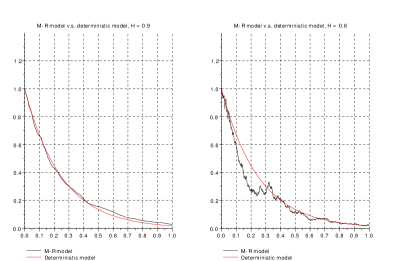
Figure 1. GM-R model v.s. deterministic model currently used

On one hand, remark that the stochastic model (black) keeps the trend of the deterministic model (red). On the other hand, remark that when the Hurst parameter is relatively close to $1$ ($H=0.9$), perturbations in biological processes are taken in account by $C$, but more realistically than for $H=0.6$.

In the sequel, we also consider the process $Z=X^{1-\beta}$. Its covariance function is denoted by $c_{Z}$.

For clinical applications, parameters $K_{e}$, $\sigma$ and $\beta$ have to be estimated. Consider a dissection $(t_{0},\dots,t_{n})$ of $[0,T]$ for $n\in\mathbb{N}^{*}$. We also put $x_{i}=X_{t_{i}}$ and $z_{i}=Z_{t_{i}}$ for $i=0,\dots,n$. The following proposition provides the likelihood function of $(x_{1},\dots,x_{n})$ which can be approximatively maximized with respect to the parameter $\theta=(K_{e},\sigma,\beta)$ by various numerical methods (not studied in this paper) :

Proposition 5.1.

Under assumptions 1.1 and 2.8, the likelihood function of $(x_{1},\dots,x_{n})$ is given by :

$$L(\theta;x_{1},\dots,x_{n})=\frac{2^{n}(1-\beta)^{n}\mathbf{1}_{x_{1}>0,\dots,x_{n}>0}}{(2\pi)^{n/2}\sqrt{\left|\det\left[\Gamma(\theta)\right]\right|}}\exp\left[-\frac{1}{2}\langle\Gamma^{-1}(\theta)U_{n}^{x},U_{n}^{x}\rangle\right]\prod_{i=1}^{n}x_{i}^{-\beta}$$

where, $\sigma^{2}(\theta)=\textrm{Var}(z_{1},\dots,z_{n})$,

$$\Gamma(\theta)=\begin{bmatrix}\sigma_{1}^{2}(\theta)&\dots&c_{Z}(t_{1},t_{n})\\ \vdots&\ddots&\vdots\\ c_{Z}(t_{n},t_{1})&\dots&\sigma_{n}^{2}(\theta)\end{bmatrix}\textrm{ and }U_{n}^{x}=\begin{pmatrix}x_{1}^{1-\beta}-C_{0}^{1-\beta}e^{-K_{e}(1-\beta)t_{1}}\\ \vdots\\ x_{n}^{1-\beta}-C_{0}^{1-\beta}e^{-K_{e}(1-\beta)t_{n}}\end{pmatrix}.$$

Proof.

Since $\tilde{W}$ is a centered Gaussian process as a Wiener integral against $W$ ; $(z_{1},\dots,z_{n})$ is a centered Gaussian vector with covariance matrix $\Gamma(\theta)$. We denote by $f_{1,\dots,n}(\theta;.)$ the natural density of $(z_{1},\dots,z_{n})$ with respect to Lebesgue’s measure on $(\mathbb{R}^{n},\mathcal{B}(\mathbb{R}^{n}))$.

Consider an arbitrary Borel bounded map $\varphi:\mathbb{R}^{n}\rightarrow\mathbb{R}$. By the transfer theorem :

$$\mathbb{E}[\varphi(x_{1},\dots,x_{n})] = \mathbb{E}[\varphi(|z_{1}|^{\gamma+1},\dots,|z_{n}^{\gamma+1}|)]$$

$$= 2^{n}\int_{\mathbb{R}_{+}^{n}}\varphi(a_{1}^{\gamma+1},\dots,a_{n}^{\gamma+1})f_{1,\dots,n}(\theta;a_{1},\dots,a_{n})da_{1}\dots da_{n}$$

by reduction to canonical form of quadratic forms.

Put $u_{i}=a_{i}^{\gamma+1}$ for $a_{i}\in\mathbb{R}_{+}^{*}$ and $i=1,\dots,n$. Then,

$$(a_{1},\dots,a_{n})=(u_{1}^{\frac{1}{\gamma+1}},\dots,u_{n}^{\frac{1}{\gamma+1}})\textrm{ and }\left|J(u_{1},\dots,u_{n})\right|=\frac{1}{(\gamma+1)^{n}}\prod_{i=1}^{n}u_{i}^{-\frac{\gamma}{\gamma+1}}$$

where, $J(u_{1},\dots,u_{n})$ denotes the Jacobian of :

$$(u_{1},\dots,u_{n})\in(\mathbb{R}_{+}^{*})^{n}\longmapsto(u_{1}^{\frac{1}{\gamma+1}},\dots,u_{n}^{\frac{1}{\gamma+1}}).$$

By applying that change of variable :

$$\mathbb{E}[\varphi(x_{1},\dots,x_{n})] = \frac{2^{n}}{(\gamma+1)^{n}}\int_{\mathbb{R}_{+}^{n}}du_{1}\dots du_{n}\varphi(u_{1},\dots,u_{n})\times$$

$$f_{1,\dots,n}(\theta;u_{1}^{\frac{1}{\gamma+1}},\dots,u_{n}^{\frac{1}{\gamma+1}})\prod_{i=1}^{n}u_{i}^{-\frac{\gamma}{\gamma+1}}.$$

Therefore, $\mathbb{P}_{(x_{1},\dots,x_{n})}(\theta;du_{1},\dots,du_{n})=L(\theta;u_{1},\dots,u_{n})du_{1}\dots du_{n}$ with :

$$L(\theta;u_{1},\dots,u_{n}) = \frac{2^{n}}{(\gamma+1)^{n}}f_{1,\dots,n}(\theta;u_{1}^{\frac{1}{\gamma+1}},\dots,u_{n}^{\frac{1}{\gamma+1}})\prod_{i=1}^{n}u_{i}^{-\frac{\gamma}{\gamma+1}}\mathbf{1}_{u_{1}>0,\dots,u_{n}>0}$$

$$= \frac{2^{n}(1-\beta)^{n}\mathbf{1}_{u_{1}>0,\dots,u_{n}>0}}{(2\pi)^{n/2}\sqrt{\left|\det\left[\Gamma(\theta)\right]\right|}}\exp\left[-\frac{1}{2}\langle\Gamma^{-1}(\theta)U_{n}^{u},U_{n}^{u}\rangle\right]\prod_{i=1}^{n}u_{i}^{-\beta}.$$

∎

Finally, consider a random time $\tau\in[0,\tau_{0}^{1}\wedge T]$ and a deterministic function $F:\mathbb{R}_{+}\rightarrow\mathbb{R}$ satisfying the following assumption :

Assumption 5.2.

The function $F$ belongs to $C^{1}(\mathbb{R}_{+};\mathbb{R})$ and there exists $(K,N)\in\mathbb{R}_{+}^{*}\times\mathbb{N}^{*}$ such that :

$$\forall r\in\mathbb{R}_{+}\textrm{, }|F(r)|\leqslant K(1+r)^{N}\textrm{ and }|\dot{F}(r)|\leqslant K(1+r)^{N}.$$

Let show the existence and compute the sensitivity of $f_{\tau}(x)=\mathbb{E}[F(C_{\tau}^{x})]$ to variations of the initial concentration $x>0$ in compartment $E$.

Proposition 5.3.

Under assumptions 1.1, 2.8 and 5.2, the function $f_{\tau}$ is differentiable on $\mathbb{R}_{+}^{*}$ and,

$$\forall x>0\textrm{, }\dot{f}_{\tau}(x)=x^{-\beta}\mathbb{E}\left[e^{-K_{e}\tau}\dot{F}(C_{\tau}^{x})(x^{1-\beta}+\tilde{W}_{\tau})^{\gamma}\right].$$

Proof.

First of all, the function $x\in\mathbb{R}_{+}^{*}\mapsto C_{\tau}^{x}$ is almost surely $C^{1}$ on $\mathbb{R}_{+}^{*}$ and,

$$\forall x>0\textrm{, }\partial_{x}C_{\tau}^{x}=x^{-\beta}\left(x^{1-\beta}+\tilde{W}_{\tau}\right)^{\gamma}e^{-K_{e}\tau}.$$

Consider $x>0$ and $\varepsilon\in]0,1]$.

On one hand, since $F$ belongs to $C^{1}(\mathbb{R}_{+};\mathbb{R})$, from Taylor’s formula :

$$\left|\frac{F(C_{\tau}^{x+\varepsilon})-F(C_{\tau}^{x})}{\varepsilon}\right| = \left|\int_{0}^{1}\dot{F}(C_{\tau}^{x+\theta\varepsilon})\partial_{x}C_{\tau}^{x+\theta\varepsilon}d\theta\right|$$

$$\leqslant \sup_{\theta\in[0,1]}K(1+\|C^{x+\theta\varepsilon}\|_{\infty;T})^{N}|\partial_{x}C_{\tau}^{x+\theta\varepsilon}|$$

by Assumption 5.2.

On the other hand, since $\theta,\varepsilon\in[0,1]$ :

(31) $$\|C^{x+\theta\varepsilon}\|_{\infty;T}\leqslant\left[(x+1)^{1-\beta}+\|\tilde{W}\|_{\infty;T}\right]^{\gamma+1}$$

and

(32) $$|\partial_{x}C_{\tau}^{x+\theta\varepsilon}|\leqslant x^{-\beta}\left[(x+1)^{1-\beta}+\|\tilde{W}\|_{\infty;T}\right]^{\gamma}.$$

By Fernique’s theorem, the right hand sides of inequalities (31) and (32) belong to $L^{p}(\Omega)$ for every $p>0$. Moreover, these upper-bounds are not depending on $\theta$ and $\varepsilon$.

Therefore, by Lebesgue’s theorem, $f_{\tau}$ is derivable at point $x$ and,

$$\dot{f}_{\tau}(x)=x^{-\beta}\mathbb{E}\left[e^{-K_{e}\tau}\dot{F}(C_{\tau}^{x})(x^{1-\beta}+\tilde{W}_{\tau})^{\gamma}\right].$$

∎

There is probably many ways to use that result in medical treatments. For example, assume that $f_{\tau}(x)$ modelize a part of patient’s therapeutic response to the administered drug. Proposition 5.3 provides a way to minimize the initial dose for an optimal response.

Remarks :

1. By the strong law of large numbers, there exists an almost surely converging estimator for that sensitivity.

2. For any $x>0$, one can show the existence of a stochastic process $h^{x}$ defined on $[0,T]$ such that $\dot{f}_{\tau}(x)=\mathbb{E}[F(C_{\tau}^{x})\delta(h^{x})]$ where, $\delta$ denotes the divergence operator associated to the Gaussian process $W$. Then, $F$ has not to be derivable anymore by assuming that $F\in L^{2}(\mathbb{R}_{+}^{*})$. It is particularly useful if $F$ is not continuous at some points.
   
   We don’t develop it in that paper because the Malliavin calculus framework has to be introduced before. To understand that idea, please refer to E. Fournié et al. [7] in Brownian motion’s case and N. Marie [18].

References

- [1] R.J. Adler. An Introduction to Continuity, Extrema, and Related Topics for General Gaussian Processes. Institute of Mathematical Statistics, Lecture Notes-Monograph Series, Vol. 12, 1990.
- [2] L. Coutin. Rough Paths via Sewing Lemma. ESAIM : Probability and Statistics, doi:10.1051/ps/2011108.
- [3] A. Dembo and O. Zeitouni. Large Deviations Techniques and Applications. Applications of Mathematics, Vol. 38, New-York. Springer-Verlag, 1998.
- [4] M. Delattre and M. Lavielle. Pharmacokinetics and Stochastic Differential Equations : Model and Methodology. Annual Meeting of the Population Approach Group in Europe, 2011.
- [5] H. Doss. Liens entre équations différentielles stochastiques et ordinaires. C.R. Acad. Sci. Paris Ser. A-B, 283(13):Ai, A939-A942, 1976.
- [6] J. Feng, J-P. Fouque and R. Kumar. Small-Time Asymptotics for Fast Mean-Reverting Stochastic Volatility Models. arXiv (1009.2782), 2010.
- [7] E. Fournié, J-M. Lasry, J. Lebuchoux, P-L. Lions and N. Touzi. Applications of Malliavin Calculus to Monte-Carlo Methods in Finance. Finance Stochast. 3, 391-412, 1999.
- [8] P. Friz and N. Victoir. Multidimensional Stochastic Processes as Rough Paths : Theory and Applications. Cambridge Studies in Applied Mathematics, 120. Cambridge University Press, Cambridge, 2010.
- [9] Y. Jacomet. Pharmacocinétique. Cours et Exercices. Université de Nice, U.E.R. de Médecine, Service de pharmacologie expérimentale et clinique, Ellipses, 1989.
- [10] S. Karlin and H.M. Taylor. A Second Course in Stochastic Processes. Academic Press Inc., Harcourt Brace Jovanovich Publishers, 1981.
- [11] K. Kalogeropoulos, N. Demiris and O. Papaspiliopoulos. Diffusion-driven Models for Physiological Processes. International Workshop on Applied Probability (IWAP), 2008.
- [12] M. Ledoux. Isoperimetry and Gaussian Analysis. Ecole d’été de probabilité de Stain-Flour, 1994.
- [13] A. Lejay. Controlled Differential Equations as Young Integrals : A Simple Approach. Journal of Differential Equations 248, 1777-1798, 2010.
- [14] T. Lyons and Z. Qian. System Control and Rough Paths. Oxford University Press, 2002.
- [15] F. Malrieu. Convergence to Equilibrium for Granular Media Equations and their Euler Schemes. Annals of Applied Probability, Vol. 13, no. 2, 540-560, 2003.
- [16] F. Malrieu et D. Talay. Concentration Inequalities for Euler Schemes. Springer-Verlag, 355-371, 2006.
- [17] X. Mao, A. Truman and C. Yuan. Euler-Maruyama Approximations in Mean-Reverting Stochastic Volatility Model under Regime-Switching. Journal of Applied Mathematics and Stochastic Analysis, 2006.
- [18] N. Marie. Sensitivities via Rough Paths. arXiv (1108.0852), 2011.
- [19] J. Neveu. Processus aléatoires gaussiens. Presses de l’Université de Montréal, 1968.
- [20] D. Nualart. The Malliavin Calculus and Related Topics. Second Edition. Probability and Its Applications, Springer, 2006.
- [21] N. Tien Dung. Fractional Geometric Mean Reversion Processes. Journal of Mathematical Analysis and Applications, vol. 330. pp. 396-402, 2011.
- [22] M. Sanz-Solé and I. Torrecilla-Tarantino. A Large Deviation Principle in Hölder Norm for Multiple Fractional Integrals. arXiv (0702049), 2007.
- [23] N. Simon. Pharmacocinétique de population. Collection Pharmacologie médicale, Solal, 2006.
- [24] H.J. Sussman. On the Gap between Deterministic and Stochastic Ordinary Differential Equations. Ann. Probability, 6(1):19-41, 1978.
- [25] F. Wu, X. Mao and K. Chen. A Highly Sensitive Mean-Reverting Process in Finance and the Euler-Maruyama Approximations. Journal of Mathematical Analysis and Applications, 348(1). pp. 540-554, 2008.