Abstract

Equipped with concrete examples of Type IIB orientifolds featuring poly-instanton corrections to the superpotential, the effects on moduli stabilization and inflationary cosmology are analyzed. Working in the framework of the LARGE volume scenario, the Kähler modulus related to the size of the four-cycle supporting the poly-instanton contributes sub-dominantly to the scalar potential. It is shown that this Kähler modulus gets stabilized and, by displacing it from its minimum, can play the role of an inflaton. Subsequent cosmological implications are discussed and compared to experimental data.

1 Introduction

For relating string compactifications to realistic four-dimensional physics, the understanding of moduli stabilization is a very central issue and has been under intense investigation for more than a decade. In order to quantitatively address certain aspects of cosmology and of particle physics, moduli stabilization is a prerequisite, as on the one hand some physical parameters depend on the value of the moduli and on the other hand the existence of unstabilized and therefore massless scalars is incompatible with observations.

Motivated by these issues, quite some progress concerning mechanisms to stabilize these moduli has been made over the past years [1, 2, 3, 4, 5, 6]. In the framework of Type IIB orientifold compactifications with $O7$ and $O3$-planes, one can distinguish two classes of models, namely the so-called KKLT models [4] and the LARGE volume scenarios [5]. Both of them successfully stabilize the moduli via (non-)perturbative effects through a two-step strategy. First, one stabilizes the complex structure moduli as well as the axio-dilaton modulus via a dominant perturbative contribution. Second, the Kähler moduli are stabilized via a sub-dominant non-perturbative contribution.

More concretely, in KKLT models, the complex structure moduli as well as the axio-dilaton are stabilized via contributions to the superpotential that are generated by turning on tree-level background fluxes [3]. On the other hand the Kähler moduli are stabilized via non-perturbative effects coming from gaugino-condensation or Euclidean $D3$-brane (short $E3$-brane) instantons [7]. These effects are sufficient to fix all closed string moduli (at least for simple setups) in a supersymmetric $AdS$ minimum, which can be uplifted to a non-supersymmetric metastable $dS$ minimum by the inclusion of $\overline{D3}$-branes [4].

Though being very nice and simple, a problematic issue is that KKLT models suffer from a lack of control over additional corrections. In particular, this is improved in the LARGE volume scenarios [5], where the inverse of the volume serves as a controllable expansion parameter. Here, one includes perturbative ${\alpha^{\prime}}^{3}$-corrections (of [8]) in the Kähler potential, leading to a new non-supersymmetric $AdS$ minimum where the modulus controlling the size of the instanton $\tau_{s}$ and the overall volume modulus ${\cal V}$ are stabilized at hierarchically separated values such that $\tau_{s}\sim\ln{\cal V}$. Thus, the basic idea is to balance a non-perturbative correction to the superpotential against a perturbative correction to the Kähler potential. Unlike KKLT models, even for generic choices of background fluxed with $W_{0}\sim{\cal O}(1)$, the overall Calabi-Yau volume is sufficient to suppress the higher derivative effects and at the same time to stabilize (all) divisor volumes. The $AdS$-minima in the large volume limit can then be uplifted making use of any of the known uplifting mechanisms [4, 9, 10, 11, 12].

Equipped with such a working framework of moduli stabilization, one is conceptually able to also address cosmological issues like realizing inflation. The central requirement for this purpose is to identify a scalar which could play the role of the inflaton field, i.e. its effective scalar potential has to admit a slow-roll region. In this respect, those “moduli” that have a flat potential at leading order and only by a sub-leading effect receive their dominant contribution are of interest. Besides sub-leading perturbative effects also instanton effects can be relevant(see [3, 7, 8, 13, 14] and references therein).

Although the concept of inflation has been proposed quite some time ago as a solution to certain cosmological problems [15, 16], the embedding of inflationary scenarios into semi-realistic string models is quite a recent development. Such an inflationary model has been initiated in [17] in which, following the idea of [18], an open string modulus appearing as brane separation was argued to be an inflaton candidate. There has been a large amount of work dedicated to build sophisticated models of open string inflation [17, 19, 20], however in particular in the framework of LARGE volume scenarios, closed string moduli inflation has also been seriously considered with a successful and consistent implementation of the observational data [21, 22, 23, 24]. Models based on the $C_{4}$ axion-moduli have also been considered for cosmological implications [25, 26, 27], whereas models with odd-axions $B_{2},C_{2}$, though also interesting, are less studied [28, 29, 30, 31]. All these string (inspired) inflationary models experience significant constraints from experimental observations, i.e. from the measurements of the temperature fluctuation in the cosmic microwave background (CMB). This includes the COBE, WMAP and Planck-satellite missions.

Along the lines of moduli getting lifted by sub-dominant contributions, recently so-called poly-instanton corrections became of interest. These are sub-leading non-perturbative contributions which can be briefly described as instanton corrections to instanton actions. These were introduced and systematically studied in the framework of Type I string compactifications in [32] and have also been analyzed in the T-dual context of Type I’ string models, where they map to BPS $D0$-branes running in loops [33]. The analogous poly-instanton effects will also appear in the Type IIB orientifolds with $O7$ and $O3$ planes. Utilizing these poly-instanton effects, moduli stabilization and inflation have been studied in a series of papers [34, 35, 36, 37, 38]. However the analysis had to be carried out from a rather heuristic point of view, as a clear understanding of the string-theoretic conditions for the generation of these effects was lacking. In this context, in the recent work [39], we have clarified the zero mode conditions for an Euclidean D3-brane instanton, wrapping a divisor of the threefold, to generate such a poly-instanton effect. There we have also provided the construction of some concrete models having the right divisors to both feature the LARGE volume scenario and to support additional poly-instanton corrections. Building on these, it is the objective of this paper to study its consequences for moduli stabilization and inflation.

The article is organized as follows. In section 2, we start with a brief review of the relevant mathematical background (from [39]) exemplifying it for a concrete Type IIB orientifold model in which poly-instanton corrections are generated. In section 3 we present a systematic study of moduli stabilization. Here we distinguish two schemes, a so-called minimal one and one with a racetrack form of the superpotential. A numerical analysis leads to the existence of critical points and a hierarchy of moduli masses. In section 4 we analyze the potential of the lightest modulus to serve as an inflaton. For this purpose, we compute several inflationary parameters and compare them to the observed values. Moreover, we give a first, rough estimate of the reheating temperature. Finally in section 5 we give our conclusions followed by an appendix providing some more details on the partially quite lengthy intermediate expressions.

2 Poly-instanton corrections

Let us briefly recall some results from [39] on the contribution of poly-instantons to the superpotential in the framework of Type IIB orientifold compactifications on Calabi-Yau threefolds with $O7$- and $O3$-planes. In this case the orientifold action is given by $\Omega\sigma(-1)^{F_{L}}$, where $\sigma$ is a holomorphic, isometric involution acting on the Calabi-Yau threefold ${\cal M}$.

Generally, the notion of poly-instantons [34] means the correction of an Euclidean D-brane instanton action by other D-brane instantons. The configuration of interest in the following is that we have two instantons $a$ and $b$ with proper zero modes to generate a non-perturbative contribution to the superpotential of the form

$$\begin{split}W=A_{a}\,\text{exp}^{-S_{a}}+A_{a}A_{b}\,\text{exp}^{-S_{a}-S_{b}}+...\,,\end{split}$$ (1)

where $A_{a,b}$ are moduli dependent one-loop determinants and $S_{a,b}$ denote the classical $D$-brane instanton actions. The latter depend on different moduli due to the different zero mode structures for these two kinds of instantons.

In the framework of Type IIB orientifolds, sufficient conditions for the zero mode structures for poly-instanton corrections to the superpotential have been worked out in [39]. Both instantons, $a$ and $b$, should be $O(1)$ instantons, i.e. a single instanton placed in an orientifold invariant position with an $O(1)$ projection. This corresponds to an $SP-$type projection for a corresponding space-time filling $D7$-brane. Instanton $a$ is an Euclidean $E3$ instanton wrapping a rigid divisor $E$ in the Calabi-Yau threefold with $H^{1,0}(E,{\cal O})=H^{2,0}(E,{\cal O})=0$. Whereas, instanton $b$ is an Euclidean $E3$-brane instanton wrapping a divisor which admits a single complex Wilson line Goldstino, i.e. a so-called Wilson line divisor with equivariant cohomology $H^{*,0}(W,{\cal O})=(1_{+},1_{+},0)$ under the involution $\sigma$. Here the lower indices $\pm$ denote the even and odd cohomology. In fact, the sufficient condition for a geometric configuration to support the poly-instanton correction is that it precisely contains one Wilson line modulino in $H^{1}_{+}(E,\cal O)$.

Examples of such Wilson line divisors are $\mathbb{P}^{1}$ fibrations over two-tori. In [39] a couple of concrete Calabi-Yau threefolds, both with and without $K3$ fibration structure, were presented which featured all the requirements mentioned above. For concreteness, let us recall one of these examples, which not only admits a Wilson line divisor $W$ but also two rigid and shrinkable del Pezzo divisors. Such geometries are particularly interesting for studying moduli stabilization as they give rise to a swiss-cheese type Kähler potential, the starting point for the LARGE volume scenario [5]. The Calabi-Yau threefold $\cal M$ is given by a hypersurface in a toric variety with defining data

	$x_{1}$	$x_{2}$	$x_{3}$	$x_{4}$	$x_{5}$	$x_{6}$	$x_{7}$	$x_{8}$
2	-1	0	1	1	0	0	0	1
4	-2	0	2	2	1	0	1	0
2	-3	0	2	1	1	1	0	0
2	1	1	0	0	0	0	0	0

with Hodge numbers $(h^{21},h^{11})=(72,4)$ and the corresponding Stanley-Reisner ideal

$${\rm SR}=\left\{x_{1}\,x_{2},x_{4}\,x_{7},x_{5}\,x_{7},x_{1}\,x_{4}\,x_{8},x_{2}\,x_{5}\,x_{6},x_{3}\,x_{4}\,x_{8},x_{3}\,x_{5}\,x_{6},x_{3}\,x_{6}\,x_{8}\right\}\,.$$ (2)

More geometric data can be found in [39].

We identified two inequivalent orientifold projections $\sigma:\{x_{4}\leftrightarrow-x_{4},x_{7}\leftrightarrow-x_{7}\}$ with $h^{11}_{-}({\cal M})=0$ so that for the Wilson line divisor $W=D_{8}=\{x_{8}=0\}$ the Wilson line Goldstino is in $H_{+}^{1}(W,{\cal O})$. It was checked that the $D3$- and $D7$-brane tadpoles can be canceled. For the analysis in the following sections, we focus on the involution $x_{7}\leftrightarrow-x_{7}$. The corresponding topological data of the relevant divisors are shown in table 1.

divisor	$(h^{00},h^{10},h^{20},h^{11})$	intersection curve
$D_{7}=dP_{7}$	$(1_{+},0,0,8_{+})$	$W:C_{g=1}$
$D_{5}$	$(1_{+},0,1_{+},21_{+})$	$W:C_{g=1}$
$D_{8}=W$	$(1_{+},1_{+},0,2_{+})$	$D_{5}:C_{g=1},\ \ D_{7}:C_{g=1}$
$D_{1}=\mathbb{P}^{2}$	$(1_{+},0,0,1_{+})$	$D_{5}:C_{g=0}$

Table 1: Divisors and their equivariant cohomology under $x_{7}\leftrightarrow-x_{7}$. The first two lines are $O7$-plane components and the remaining two divisors can support $E3$ instantons. The $D_{7}$ divisor also supports gaugino condensation.

We also showed that there are no extra vector-like zero modes on the intersection of $E3\cap D7$, i.e.  all sufficient conditions were satisfied for the divisor $W$ to generate a poly-instanton correction to the non-perturbative superpotential

$$\begin{split}W&=A_{1}\,\exp\left(-2\pi T_{1}\right)+A_{1}\,A_{8}\,\exp\left(-2\pi T_{1}-2\pi T_{8}\right)+\\ &\phantom{aaaaaaaaaaa}A_{7}\,\exp\left(-a_{7}T_{7}\right)+A_{7}\,A_{8}\,\exp\left(-a_{7}T_{7}-2\pi T_{8}\right)+\ldots\;.\end{split}$$ (3)

Taking into account the Kähler cone constraints, the volume form for this model could be written in the strong swiss-cheese like form

$$\begin{split}{\cal V}&=\textstyle{\frac{1}{9}}\Bigl{(}\frac{1}{\sqrt{2}}(\tau_{1}+3\tau_{6}+6\tau_{7}+3\tau_{8})^{3/2}-\sqrt{2}\tau_{1}^{3/2}-3\tau_{7}^{3/2}-3(\tau_{7}+\tau_{8})^{3/2}\Bigr{)}\,.\end{split}$$ (4)

The above volume form shows that the large volume limit is given by $\tau_{6}\rightarrow\infty$ while keeping the other shrinkable del Pezzo four-cycles $\tau_{1,7}$ and the Wilson line four-cycle $\tau_{8}$ small. Note, all other models studied in [39] shared a similar strong swiss-cheese-like volume form with the same intriguing appearance of the Wilson line Kähler modulus.

These concrete examples motivate us now to make the following slightly simplified ansatz for the tree-level Kähler potential and the poly-instanton generated superpotential

$$\begin{split}K=-2\ln{\cal V}=-2\ln\left({\tau_{b}}^{\frac{3}{2}}-{\tau_{s}}^{\frac{3}{2}}-(\tau_{s}+\tau_{w})^{\frac{3}{2}}\right)\,,\end{split}$$ (5)

$$\begin{split}W=A_{s}\,e^{-a_{s}T_{s}}+A_{s}\,A_{w}\,\,e^{-a_{s}\,T_{s}-a_{w}\,T_{w}}\,,\end{split}$$ (6)

where $A_{s,w}$ are one-loop determinants and $a_{s,w}$ are numerical constants.

It is the objective of this paper to analyze the physical implications of such a Kähler and superpotential for moduli stabilization and inflationary cosmology.

3 Moduli stabilization

A generic orientifold compactification of Type IIB string theory leads to an effective four-dimensional ${\cal N}=1$ supergravity theory. In the closed string sector, the bosonic part of the massless chiral superfields arises from the dilaton, the complex structure and Kähler moduli and the dimensional reduction of the NS-NS and R-R $p$-form fields. The bosonic field content is given by

$$\begin{split}\tau&=C^{(0)}+ie^{-\phi}\,,\qquad U^{i}=u^{i}+iv^{i},\quad i=1\ldots h^{21}_{+}\,,\\[2.84544pt] {G}^{a}&=c^{a}-\tau{b}^{a}\,,\qquad a=1,\ldots,h^{11}_{-}\,,\\ T_{\alpha}&=\frac{1}{2}\kappa_{\alpha\beta\gamma}t^{\beta}t^{\gamma}+i\left(\rho_{\alpha}-\kappa_{\alpha ab}\,{c^{a}b^{b}}\right)+\frac{i}{2}\,\tau\kappa_{\alpha ab}b^{a}b^{b}\quad\text{~{}and}\quad\alpha=1,\ldots,h^{11}_{+}\,,\end{split}$$ (7)

where $c^{a}$ and $b^{a}$ are defined as integrals of the axionic $C^{(2)}$ and $B^{(2)}$ forms and $\rho_{\alpha}$ as integrals of $C^{(4)}$ over a basis of four-cycles $D_{\alpha}$. From now on, as in our concrete examples, we assume $h^{11}_{-}=0$.

The supergravity action is specified by the Kähler potential, the holomorphic superpotential $W$ and the holomorphic gauge kinetic function. The Kähler potential for the supergravity action is given as,

$$\hskip-28.45274ptK=-\ln\biggl{(}-i(\tau-{\bar{\tau}})\biggr{)}-\ln\left(-i\int_{\cal M}\Omega\wedge{\bar{\Omega}}\right)-2\ln\Bigl{(}{\cal V}(T_{\alpha})\Bigr{)}\,,$$ (8)

where ${\cal V}={\frac{1}{6}}{\kappa}_{\alpha\beta\gamma}t^{\alpha}t^{\beta}t^{\gamma}$ is the volume of the internal Calabi-Yau threefold.

The general form of the superpotential $W$ is given as

$$W=\int_{\cal M}G_{3}\wedge\Omega+\sum_{E}{A}_{E}(\tau,U^{i})\,e^{-a_{E}\gamma^{\alpha}\,T_{\alpha}}\,$$ (9)

with the instantonic divisor given by $E=\sum\gamma^{\alpha}D_{\alpha}$. The first term is the Gukov-Vafa-Witten (GVW) flux induced superpotential [3] and the second one denotes the non-perturbative correction coming from Euclidean $D3$-brane instantons ($a_{E}=2\pi$) and gaugino condensation on $U(N)$ stacks of $D7$-branes ($a_{E}=2\pi/N$). In terms of the Kähler potential and the superpotential the scalar potential is given by

$$\begin{split}V=e^{K}\Biggl{(}\sum_{I,\,J}{K}^{I\bar{J}}{\cal D}_{I}W{\bar{\cal D}}_{\bar{J}}{\bar{W}}-3|W|^{2}\Biggr{)}\,,\end{split}$$ (10)

where the sum runs over all moduli. As usual in the LARGE volume scenario, the complex structure moduli and the axio-dilaton are stabilized at order $1/{\cal V}^{2}$ by the GVW-superpotential. Since the stabilization of the Kähler moduli is by sub-leading terms in the ${\cal V}^{-1}$ expansion, for this purpose the complex structure moduli and the dilaton can be treated as constants.

In the remainder of this section we will analyze moduli stabilization for an effective supergravity model defined essentially by the tree-level Kähler potential (5) along with perturbative ${\alpha^{\prime}}^{3}$ correction and the non-perturbative superpotential (6). We will discuss two schemes for moduli stabilization. In the first one, up to an additional flux induced constant $W_{0}$, we will just consider the minimal superpotential (6) and in the second one we will extend the model to a racetrack-type variant.

We will see that the first scheme is problematic in the sense that the minima of the scalar potential lie outside the regime of validity of the $\alpha^{\prime}$ expansion. This is remedied in the second scheme, with the downside that one has to perform a certain tuning of the parameters.

Scheme 1: minimal

Note that, for $h^{11}_{-}=0$, the ${\cal N}=1$ Kähler coordinates are simply given as $T_{\alpha}=\tau_{\alpha}+i\rho_{\alpha}$. For the Kähler and superpotential, we choose the minimal poly-instanton motivated form

$$\begin{split}K&=-2\,\ln{\cal Y}\,,\\[5.69046pt] W&=W_{0}+A_{s}e^{-a_{s}T_{s}}+A_{s}A_{w}\,e^{-a_{s}T_{s}-a_{w}T_{w}}\,,\end{split}$$ (11)

where ${\cal Y}={\cal V}(T_{\alpha})+C_{\alpha^{\prime}}\;$ such that

$$\begin{split}{\cal Y}=\xi_{b}(T_{b}+\bar{T}_{b})^{\frac{3}{2}}-\xi_{s}(T_{s}+\bar{T}_{s})^{\frac{3}{2}}-\xi_{sw}\Bigl{(}(T_{s}+\bar{T}_{s})+(T_{w}+\bar{T}_{w})\Bigr{)}^{\frac{3}{2}}+C_{\alpha^{\prime}}\,.\end{split}$$ (12)

Here, $C_{\alpha^{\prime}}$ denotes the perturbative ${\alpha^{\prime}}^{3}$-correction given as

$$\begin{split}C_{\alpha^{\prime}}=-\frac{\chi({\cal M})\,({{\tau}-\bar{\tau}})^{\frac{3}{2}}\zeta(3)}{4(2\pi)^{3}\,({2i})^{\frac{3}{2}}}\end{split}$$ (13)

with $\chi({\cal M})$ being the Euler characteristic of the Calabi-Yau. The large volume limit is defined by taking $\tau_{b}\rightarrow\infty$ while keeping the other divisor volumes small. Note that the above volume form is very similar to the one of ‘strong’ swiss-cheese type.

The effective scalar potential for the set of moduli $\{T_{b},T_{s},T_{w}\}$ can be expressed in terms of three types of contributions

$$\begin{split}V(\tau_{b},\tau_{s},\tau_{w},\rho_{s},\rho_{w})\equiv V({\cal V},\tau_{s},\tau_{w},\rho_{s},\rho_{w})=V_{\alpha^{\prime}}+V_{\rm np1}+V_{\rm np2}\,.\end{split}$$ (14)

In the large volume limit, the leading contributions are

$$\begin{split}V_{\alpha^{\prime}}&=\frac{3{\,{\cal C}_{\alpha^{\prime}}}\,|W_{0}|^{2}}{2{\cal V}^{3}}\,,\\[5.69046pt] V_{\rm np1}&=\frac{4\,{W_{0}}}{{\cal V}^{2}}\biggl{[}{\,{A_{s}}}\,e^{-{a_{s}\tau_{s}}-{a_{w}\,\tau_{w}}}\Bigl{(}{\,a_{s}}e^{{a_{w}\,\tau_{w}}}{\tau_{s}}\cos({\,a_{s}}{\rho_{s}})\\ &\phantom{aaaaaaaaaaaaaaaaaa}+{\,{A_{w}}}({a_{s}\tau_{s}}+{a_{w}\,\tau_{w}})\cos({\,a_{s}}{\rho_{s}}+{\,{a_{w}}}{\rho_{w}})\Bigr{)}\biggr{]}\,,\\ V_{\rm np2}&=\frac{2\sqrt{2}}{3\,\xi_{s}\,\xi_{sw}\,{\cal V}}\biggl{[}A^{2}_{s}\,a_{s}^{2}\,e^{-2({a_{s}\tau_{s}}+{a_{w}\,\tau_{w}})}\Bigl{(}\xi_{sw}\left(A^{2}_{w}+e^{2{a_{w}\tau_{w}}}\right)\sqrt{{\tau_{s}}}\\ &\phantom{aaaaaaaaaa}+2\xi_{sw}\,a_{s}\,(a_{s}-a_{w})A_{w}\,e^{a_{w}\tau_{w}}\sqrt{\tau_{s}}\cos(a_{w}\rho_{w})\\ &\phantom{aaaaaaaaaa}-2\xi_{sw}\,{a_{w}}a_{s}\,A^{2}_{w}\,\sqrt{\tau_{s}}+a^{2}_{w}\,A^{2}_{w}\left(\xi_{s}\,\sqrt{{\tau_{s}}+{\tau_{w}}}+\xi_{sw}\sqrt{\tau_{s}}\right)\Bigr{)}\biggr{]}\,.\end{split}$$ (15)

In the absence of poly-instanton corrections the above scalar potential reduces to

$$\begin{split}V^{\rm LVS}({\cal V},\tau_{s},\rho_{s})=&\frac{2{\sqrt{2}}\,a_{s}^{2}\,A_{s}^{2}\,e^{-2{a_{s}\tau_{s}}}\sqrt{{\tau_{s}}}}{3\,\xi_{s}\,{\cal V}}+\frac{{4\,a_{s}}{\,{A_{s}}}\,e^{-{a_{s}\tau_{s}}}\,{\tau_{s}}\cos(a_{s}\rho_{s}){W_{0}}}{{\cal V}^{2}}\\[2.84544pt] &+\frac{3{\,{\cal C}_{\alpha^{\prime}}}\,|W_{0}|^{2}}{2\,{\cal V}^{3}}\end{split}$$ (16)

which corresponds to the potential of the standard single-hole LARGE volume scenario [5]. The extrema of the above scalar potential can be collectively described by the following three hypersurfaces in moduli space

$$\begin{split}a_{s}\overline{\rho}_{s}&=N\pi\,,\qquad{\cal C}_{\alpha^{\prime}}=\frac{32\sqrt{2}a_{s}\,\xi_{s}\,\overline{\tau}_{s}^{\frac{5}{2}}(-1+a_{s}\overline{\tau}_{s})}{(-1+4a_{s}\overline{\tau}_{s})^{2}}\,,\\[2.84544pt] W_{0}&=-\frac{\,a_{s}A_{s}\,e^{-a_{s}\overline{\tau}_{s}}\,\overline{\cal V}\,(-1+4a_{s}\overline{\tau}_{s})}{6\,{\sqrt{2}}\,\xi_{s}\,\sqrt{\overline{\tau}_{s}}\,(-1+a_{s}\overline{\tau}_{s})}\,.\end{split}$$ (17)

From the above, one finds that $\tau_{s}$ gets stabilized in terms of the $\alpha^{\prime}$-correction term in the scalar potential, i.e. $\overline{\tau}_{s}\sim(C_{\alpha^{\prime}})^{2/3}$. Then ${\cal V}$ gets stabilized at an exponential large volume $\overline{\cal V}\sim\exp(a_{s}\,\overline{\tau}_{s})$. The form of the scalar potential is shown in figure 1.

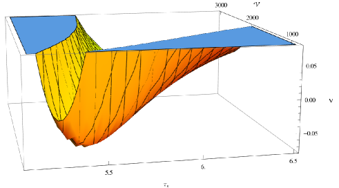
Figure 1: The scalar potential $V({\cal V},\tau_{s})$ (multiplied by $10^{7}$) as a function of ${\cal V}$ and $\tau_{s}$ in the absence of poly-instanton effects. The model dependent parameters have been chosen to be $\chi({\cal M})=-136$, $\xi_{b}=\frac{1}{36}$, $\xi_{s}=\xi_{sw}=\frac{1}{6\sqrt{2}}$, $a_{s}=\frac{2\pi}{4}$, $A_{s}=8$, $g_{s}=0.12$, $W_{0}=-5$. The respective minimum values for the moduli are $\overline{\rho}_{s}=0$, $\overline{\tau}_{s}=5.44$, $\overline{\cal V}=1086$.

In addition to the standard LARGE volume scenario terms (16), the generic potential (15) involves sub-dominant contributions. These are further suppressed by powers of $e^{-a_{w}\tau_{w}}$. Collecting the sub-leading terms of type $e^{-a_{w}\tau_{w}}$, we find

$$\begin{split}V(\tau_{b},\tau_{s},\tau_{w},\rho_{s},\rho_{w})=V^{\rm LVS}({\cal V},\tau_{s},\rho_{s})+V(\tau_{w},\rho_{w})\,,\end{split}$$ (18)

where

$$\begin{split}V(\tau_{w},\rho_{w})\sim&\frac{4\,A_{s}\,A_{w}\,(a_{s}\tau_{s}+a_{w}\tau_{w})\,e^{-a_{s}\tau_{s}-a_{w}\tau_{w}}\,W_{0}\,\cos(a_{s}\rho_{s}+a_{w}\rho_{w})}{{\cal V}^{2}}\\[2.84544pt] &+\frac{2\sqrt{2}\,a_{s}(a_{s}-a_{w})\,A_{s}^{2}\,A_{w}\,{\sqrt{\tau}_{s}}\,e^{-2a_{s}\tau_{s}-a_{w}\tau_{w}}\,\cos(a_{w}\rho_{w})}{3\,\xi_{s}\,{\cal V}}\,.\end{split}$$ (19)

Thus, the Kähler moduli $\tau_{b}$ and $\tau_{s}$ are stabilized as in the standard LARGE volume scenario at order ${\cal V}^{-3}$. At this order, the modulus $\tau_{w}$ remains a flat direction. This makes it a natural candidate for realizing slow-roll inflation. The Wilson-line divisor volume $\tau_{w}$ gets lifted once the sub-dominant poly-instanton effects are included. Moreover, with lifting the flatness via a sub-dominant correction, one usually expects that the mass-hierarchy will be maintained during the motion of the lightest modulus while keeping the heavier ones at their minimum.

Now, assuming that the single field approximation is a valid description and after stabilizing the heavier moduli $\tau_{b},\tau_{s}$ (and the relevant axion moduli) at their respective minima by solving (17), the sub-leading scalar potential for $\tau_{w}$ is given by

$$V(\tau_{w})=V^{\rm LVS}(\overline{\cal V},\overline{\tau}_{s},\overline{\rho}_{s})+\,e^{-a_{w}\tau_{w}}\,\bigl{(}\gamma_{1}+\gamma_{2}\tau_{w}\bigr{)}\,,$$ (20)

where the constants $\gamma_{1,2}$ are

$$\begin{split}\gamma_{1}&=\frac{\gamma_{2}\,\overline{\tau}_{s}\,\bigl{(}a_{s}(3+4a_{w}\overline{\tau}_{s})-4a_{w}\bigr{)}}{a_{w}(-1+4a_{s}\overline{\tau}_{s})}\,,\\[5.69046pt] \gamma_{2}&=\frac{24{\sqrt{2}}\,A_{w}\,a_{w}\,\xi_{s}\,|W_{0}|^{2}\,{\sqrt{\overline{\tau}_{s}}}(-1+a_{s}\overline{\tau}_{s})}{a_{s}\,\overline{\cal V}^{3}\,(1-4a_{s}\overline{\tau}_{s})}\,.\end{split}$$ (21)

The minimization condition for $\tau_{w}$ boils down to

$$\partial_{\tau_{w}}V({\tau_{w}})|_{\overline{\tau}_{w}}=0\Rightarrow a_{w}\overline{\tau}_{w}=1+\frac{\overline{\tau}_{s}\bigl{(}a_{s}(3+4a_{w}\overline{\tau}_{s})-4a_{w}\bigr{)}}{1-4a_{s}\overline{\tau}_{s}}\,,$$ (22a)

$$\partial^{2}_{\tau_{w}}V({\tau_{w}})|_{\overline{\tau}_{w}}=\frac{24\sqrt{2}a_{w}^{2}\,A_{w}\,\xi_{s}\,|W_{0}|^{2}\,\sqrt{\overline{\tau}_{s}}\,(-1+a_{s}\overline{\tau}_{s})\,e^{-a_{w}\overline{\tau}_{w}}}{a_{s}\,\overline{\cal V}^{3}\,(-1+4a_{s}\overline{\tau}_{s})}>0\,.$$ (22b)

Now we observe that, for the natural values $a_{s}=2\pi=a_{w}$ and $\overline{\tau}_{s}>1$, one obtains $\overline{\tau}_{w}<0$. Even though, for $a_{s}=\frac{2\pi}{n_{a}},a_{w}=2\pi$ with appropriate value of $n_{a}$ and a marginally trustable value of $\overline{\tau}_{s}$, it might be possible to get a positive value of $\overline{\tau}_{w}$, it turns out that still $\overline{\tau}_{w}<1$. Thus, we conclude that in this scheme $\tau_{w}$ gets stabilized outside the range of validity of the leading order low-energy effective action. Therefore, this minimum is not trustable.

Scheme 2: racetrack

In this section, we will perform a similar analysis for a racetrack type extension of the superpotential. The intention is that this introduces more parameters into the problem, increasing the chances that, for certain choice(s) of a set of parameters, trustable minima for the volume of the Wilson line divisor can be found. The poly-instanton corrected racetrack superpotential takes the form

$$\begin{split}W=W_{0}+A_{s}\,e^{-a_{s}T_{s}}+A_{s}A_{w}\,e^{-a_{s}T_{s}-a_{w}T_{w}}-B_{s}\,e^{-b_{s}T_{s}}-B_{s}B_{w}\,e^{-b_{s}T_{s}-b_{w}T_{w}}\,.\end{split}$$ (23)

The generic form of the induced scalar potential can be found in eq.(66) in appendix B. Now, we proceed with the same two step strategy for studying Kähler moduli stabilization as done in the previous section.

In the large volume limit, the most dominant contributions to the generic scalar potential ${\bf V}(\tau_{b},\tau_{s},\tau_{w},\rho_{s},\rho_{w})$ are again collected by three types of terms. In the absence of poly-instanton effects, they simplify to

$$\begin{split}{\bf V}({\cal V},\tau_{s},\rho_{s})\simeq{\bf V}_{\alpha^{\prime}}({\cal V})+{\bf V}_{\rm np1}({\cal V},\tau_{s},\rho_{s})+{\bf V}_{\rm np2}({\cal V},\tau_{s},\rho_{s})\,,\end{split}$$ (24)

where

$$\hskip-22.76228pt{\bf V}_{\alpha^{\prime}}=\frac{3{\,{\cal C}_{\alpha^{\prime}}}\,|W_{0}|^{2}}{2\,{\cal V}^{3}}\,,$$

$$\hskip-22.76228pt{\bf V}_{\rm np1}=\frac{4\,a_{s}\,{A_{s}}\,W_{0}\,e^{-\,a_{s}{\tau_{s}}}\,{\tau_{s}}\cos(\,a_{s}{\rho_{s}})}{{\cal V}^{2}}-\frac{4\,b_{s}\,{B_{s}}\,W_{0}\,e^{-\,b_{s}{\tau_{s}}}\,{\tau_{s}}\cos(\,b_{s}{\rho_{s}})}{{\cal V}^{2}}\,,$$ (25)

$$\hskip-22.76228pt{\bf V}_{\rm np2}=\frac{2\sqrt{2}\,a_{s}^{2}\,A_{s}^{2}\,e^{-2\,a_{s}{\tau_{s}}}\sqrt{{\tau_{s}}}}{3\,\xi_{s}\,{\cal V}}-\frac{4\sqrt{2}\,a_{s}\,b_{s}\,{A_{s}}\,{B_{s}}\,e^{-(\,a_{s}+\,b_{s}){\tau_{s}}}\sqrt{{\tau_{s}}}\cos\bigl{(}(\,a_{s}-\,b_{s}){\rho_{s}}\bigr{)}}{3\,\xi_{s}\,{\cal V}}$$

$$\hskip 17.07182pt+\frac{2\sqrt{2}\,b_{s}^{2}\,B_{s}^{2}\,e^{-2\,b_{s}{\tau_{s}}}\sqrt{{\tau_{s}}}}{3\,\xi_{s}\,{\cal V}}\,.$$

The above scalar potential reduces to (16) for $B_{s}=0$. Moreover, as expected, the potential (3) does not depend on the Wilson line divisor volume modulus $\tau_{w}$. Therefore, at this stage it remains a flat-direction to be lifted via sub-dominant poly-instanton effects.

The extremality conditions $\partial_{{\cal V}}{\bf V}=\partial_{{\tau_{s}}}{\bf V}=\partial_{{\rho_{s}}}{\bf V}=0$ are collectively given as

$$\begin{split}W_{0}&=\frac{\overline{\cal V}\,(b_{s}\overline{\lambda}_{2}-a_{s}\overline{\lambda}_{1})\,\Bigl{[}b_{s}\overline{\lambda}_{2}(-1+4b_{s}\overline{\tau}_{s})-a_{s}\overline{\lambda}_{1}(-1+4a_{s}\overline{\tau}_{s})\Bigr{]}}{6\sqrt{2}\,\xi_{s}\,\sqrt{\overline{\tau}_{s}}\Bigl{[}b_{s}\overline{\lambda}_{2}(-1+b_{s}\overline{\tau}_{s})-a_{s}\overline{\lambda}_{1}(-1+a_{s}\overline{\tau}_{s})\Bigr{]}}\,,\\[5.69046pt] {\cal C}_{\alpha^{\prime}}&=\frac{32\sqrt{2}\,\xi_{s}\,\overline{\tau}_{s}^{\frac{5}{2}}(b_{s}^{2}\,\overline{\lambda}_{2}-a_{s}^{2}\,\overline{\lambda}_{1})\,\Bigl{[}b_{s}\overline{\lambda}_{2}(-1+b_{s}\overline{\tau}_{s})-a_{s}\overline{\lambda}_{1}(-1+a_{s}\overline{\tau}_{s})\Bigr{]}}{\Bigl{[}a_{s}\overline{\lambda}_{1}(-1+4a_{s}\overline{\tau}_{s})-b_{s}\overline{\lambda}_{2}(-1+4b_{s}\overline{\tau}_{s})\Bigr{]}^{2}}\,,\\[5.69046pt] a_{s}\,\overline{\rho}_{s}&=N\pi\quad{\rm with}\quad\overline{\lambda}_{1}=A_{s}\,e^{-a_{s}\overline{\tau}_{s}}\quad\text{~{}and~{}}\ \ \overline{\lambda}_{2}=B_{s}\,e^{-b_{s}\overline{\tau}_{s}}\;.\end{split}$$ (26)

One finds that $\tau_{s}$ gets stabilized in terms of $C_{\alpha^{\prime}}$ as $\overline{\tau}_{s}\sim({C_{\alpha^{\prime}}})^{\frac{2}{3}}$ and then ${\cal V}$ gets stabilized via an exponential term $\exp(a_{s}\tau_{s})$ (encoded in $\lambda_{i}$’s) so that the overall volume of the Calabi-Yau threefold is exponentially large. The intersection of the above three hypersurfaces in the moduli space of $\{\tau_{b},\tau_{s},\rho_{s}\}$ determines the critical point(s) of the scalar potential. These equations are hard to solve analytically, however a numerical analysis gives the behavior of the scalar potential as shown in figure 2.

Now, in addition to the leading order standard racetrack terms (3), the generic potential (66) involves sub-dominant contributions, which are further suppressed by powers of $\exp(-a_{w}\tau_{w})$. Collecting these sub-leading terms, in the single field approximation, the effective potential for $\tau_{w}$ becomes

$$\begin{split}{\bf V}({\cal V},\tau_{s},\tau_{w},\rho_{s},\rho_{w})={\bf V}^{\rm LVS}({\cal V},\tau_{s},\rho_{s})+{\bf V}(\tau_{w},\rho_{w})\,,\end{split}$$ (27)

where, ${\bf V}^{\rm LVS}({\cal V},\tau_{s},\rho_{s})$ is the racetrack version of the standard large volume potential which stabilizes the Kähler moduli $\tau_{b}$ (or ${\cal V}$) and $\tau_{s}$ at order ${\cal V}^{-3}$ and

$$\begin{split}{\bf V}(\tau_{w},\rho_{w})&\sim\frac{4W_{0}}{\overline{\cal V}^{2}}\Bigl{[}\overline{\lambda}_{1}\,{A_{w}}\,e^{-\,{a_{w}}{\tau_{w}}}\,(a_{s}\overline{\tau}_{s}+a_{w}\tau_{w})\,\cos({a_{w}}{\rho_{w}})\\ &\phantom{aaaaaaaaaaaaaa}-\overline{\lambda}_{2}\,{B_{w}}\,e^{-{b_{w}}{\tau_{w}}}\,(b_{s}{\overline{\tau}_{s}}+b_{w}\tau_{w})\,\cos({b_{w}}{\rho_{w}})\Bigr{]}\\ &+\frac{4\sqrt{2}\,(b_{s}\overline{\lambda}_{2}-a_{s}\overline{\lambda}_{1})\,\sqrt{\overline{\tau}_{s}}}{3\,\xi_{s}\,\overline{\cal V}}\Bigl{[}\overline{\lambda}_{2}(b_{s}-b_{w})B_{w}\,e^{-b_{w}\tau_{w}}\cos(b_{w}\rho_{w})\\ &\phantom{aaaaaaaaaaaaaaaaaaaaa}-\overline{\lambda}_{1}(a_{s}-a_{w})A_{w}\,e^{-a_{w}\tau_{w}}\,\cos(a_{w}\rho_{w})\Bigr{]}\,\\ &\sim{\cal O}\left({\textstyle\frac{1}{{\cal V}^{3+p}}}\right).\end{split}$$ (28)

Here, $p$ is a positive constant and, similar to [36], it is defined such that the poly-instanton contribution to the scalar potential adds an extra multiplicative factor $\left(\frac{1}{{\cal V}^{p}}\right)$ to the scalar potential as compared to the one in the absence of poly-instanton effects.

After stabilizing the $\rho_{w}$-axion at its minimum and using $a_{w}=b_{w}$ along with eliminating $W_{0}$ via the first relation in eq.(26), the above effective scalar potential for the $\tau_{w}$ modulus can again be written in the simple form

$${\bf V}(\tau_{w})=V_{0}+e^{-a_{w}\tau_{w}}\left(\mu_{1}+\mu_{2}\tau_{w}\right)\,.$$ (29)

Here $V_{0},\mu_{1},\mu_{2}$ are constants depending on the stabilized values of the heavier moduli as

$$\begin{split}\mu_{1}&=\mu_{0}\biggl{[}4\overline{\tau}_{s}\bigl{(}(a_{s}-a_{w})A_{w}\overline{\lambda}_{1}-(b_{s}-a_{w})B_{w}\overline{\lambda}_{2}\bigr{)}\\ &+\frac{\overline{\tau}_{s}\,(b_{s}B_{w}\overline{\lambda}_{2}-a_{s}A_{w}\overline{\lambda}_{1})\,\bigl{(}a_{s}\overline{\lambda}_{1}(-1+4a_{s}\overline{\tau}_{s})-b_{s}\overline{\lambda}_{2}(-1+4b_{s}\overline{\tau}_{s})\bigr{)}}{a_{s}\overline{\lambda}_{1}(-1+a_{s}\overline{\tau}_{s})-b_{s}\overline{\lambda}_{2}(-1+b_{s}\overline{\tau}_{s})}\biggr{]}\,,\\[5.69046pt] \mu_{2}&=\mu_{0}a_{w}\left[\frac{\bigl{(}B_{w}\overline{\lambda}_{2}-A_{w}\overline{\lambda}_{1}\bigr{)}\bigl{(}a_{s}\overline{\lambda}_{1}(-1+4a_{s}\overline{\tau}_{s})-b_{s}\overline{\lambda}_{2}(-1+4b_{s}\overline{\tau}_{s})\bigr{)}}{a_{s}\overline{\lambda}_{1}(-1+a_{s}\overline{\tau}_{s})-b_{s}\overline{\lambda}_{2}(-1+b_{s}\overline{\tau}_{s})}\right]\end{split}$$ (30)

with

$$\begin{split}\mu_{0}=\frac{\sqrt{2}(\,a_{s}\overline{\lambda}_{1}-b_{s}\overline{\lambda}_{2})}{3\,\xi_{s}\,\overline{\cal V}\,\sqrt{\overline{\tau}_{s}}}\,.\end{split}$$ (31)

The extremality condition $\partial_{\tau_{w}}{\bf V}(\tau_{w})|_{\overline{\tau}_{w}}=0$ boils down to

$$a_{w}\overline{\tau}_{w}=1-a_{w}\frac{\mu_{1}}{\mu_{2}}\,,$$ (32a)

$$\partial^{2}_{\tau_{w}}{\bf V}(\tau_{w})|_{\overline{\tau}_{w}}=-a_{w}\mu_{2}\,\exp\Bigl{(}-1+\frac{a_{w}\,\mu_{1}}{\mu_{2}}\Bigr{)}>0\;.$$ (32b)

Note that, if we switch off the racetrack form in the superpotential, the $\mu_{i}$ simplify and (32a) reduces to the relation (22a) derived in the first scheme. Recall that there we were facing the problem of stabilizing $\tau_{w}$ such that we can trust the underlying effective supergravity theory.

The sole effect of including the racetrack term is that the parametrization of the $\mu_{i}$ change. Tuning the model dependent parameters makes it now possible to stabilize the modulus of the Wilson line divisor such that $\overline{\tau}_{w}>1$. Demanding that this critical point is a minimum of the effective potential, (32b) implies that the parameters are to be tuned such that $\mu_{2}$ is negative. It follows that $\mu_{1}$ has to be positive, as ${\mu_{1}/\mu_{2}}<0$ is required for stabilizing $\tau_{w}$ inside the Kähler cone.

Furthermore, the parameters $\mu_{i}$ appearing in (29) are corrected by sub-leading terms, which are suppressed by one more volume factor and hence do not induce a significant shift in the stabilized modulus $\tau_{w}$. Also, it is important to emphasize that the form of the potential (29) does not change via sub-leading contributions and only $V_{0},~{}\mu_{1}$ and $\mu_{2}$ are corrected. The analytic studies done so far are confirmed by the explicit numerical analysis to be presented in the upcoming paragraph.

Benchmark models

In table 2 we present the parameters for four benchmark models, where we have tuned the parameters such that the subsequent stabilized values for divisor volumes are within the Kähler cone and that we can trust the supergravity theory.

	$A_{s}$	$B_{s}$	$A_{w}$	$B_{w}$	$a_{s}$	$b_{s}$	$g_{s}$	$W_{0}$	$\mu_{1}$	$\frac{\mu_{2}}{\mu_{1}}$	$\frac{V_{0}}{\mu_{1}}$	$p$
${\cal B}_{1}$	3	2	0.5	1.749	$\frac{2\pi}{7}$	$\frac{2\pi}{6}$	0.12	-20	$3.0\times 10^{-8}$	$-0.7$	$-11.4$	1.84
${\cal B}_{2}$	6	0.5	0.1	4.771	$\frac{2\pi}{6}$	$\frac{2\pi}{5}$	0.10	-10	$5.8\times 10^{-10}$	$-1.0$	$-117$	1.72
${\cal B}_{3}$	8	0.8	0.1	6.5075	$\frac{2\pi}{5}$	$\frac{2\pi}{4}$	0.11	-10	$5.1\times 10^{-10}$	$-1.0$	$-85.0$	1.61
${\cal B}_{4}$	8	0.8	0.1	17.143	$\frac{2\pi}{4}$	$\frac{2\pi}{3}$	0.12	-5	$1.1\times 10^{-10}$	$-1.0$	$-62.1$	1.52

Table 2: Parameters of the benchmark models, where the other model dependent parameters are given as $\chi({\cal M})=-136$, $\xi_{b}=\frac{1}{36},~{}\xi_{s}=\xi_{sw}=\frac{1}{6\sqrt{2}},~{}a_{w}=2\pi=b_{w},$ and $\rho_{s}=0=\rho_{w}$.

In table 3 we list the values of the moduli in the minimum.

	$\overline{\tau}_{s}$	$\overline{\tau}_{w}$	$\overline{\cal V}$
${\cal B}_{1}$	5.684	1.658	905.1
${\cal B}_{2}$	6.607	1.129	941.0
${\cal B}_{3}$	5.977	1.161	1015.3
${\cal B}_{4}$	5.440	1.124	1093.2

Table 3: The stabilized values of divisor volume moduli corresponding to the respective benchmark models.

For the benchmark model ${\cal B}_{1}$, the form of the scalar potential $V({\cal V},\tau_{s})$ as a function of ${\cal V}$ and $\tau_{s}$ is shown in figure 2.

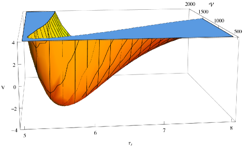
Figure 2: The scalar potential $V({\cal V},\tau_{s})$ (multiplied by $10^{7}$) vs ${\cal V}$ and $\tau_{s}$ for benchmark model ${\cal B}_{1}$ in the absence of poly-instanton effects.

For fixed values of the overall volume and of the volume of the small cycle $\tau_{s}$, the dependence of the scalar potential on $\tau_{w}$ is shown in figure 3. The respective two plots for the other benchmark models look quite similar.

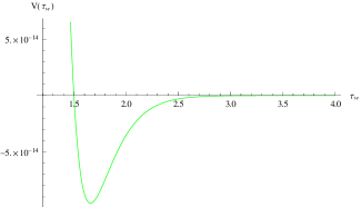
Figure 3: The effective scalar potential $V(\tau_{w})$ vs $\tau_{w}$ at stabilized value of the heavier moduli $\overline{\cal V},\overline{\tau}_{s}$ for benchmark model ${\cal B}_{1}$.

4 Inflationary cosmology

In this section we investigate whether the Wilson-line modulus $\tau_{w}$ can serve as an inflaton field. Since we are working in the framework of the LARGE volume scenario, all Kähler moduli except the overall volume mode are potential inflaton candidates. The reason is that the ${\cal N}=1$ F-term scalar potential possesses the so-called no-scale structure at tree level, which due to the perturbative $\alpha^{\prime}$-correction to the Kähler potential is broken only for the overall volume modulus. Furthermore, the expansion of the dangerous prefactor $\exp(K)$ in the F-term scalar potential (which induces higher-dimensional operators and therefore corrections to $\eta$) depends only on the overall volume of the Calabi-Yau. Therefore, in the absence of non-perturbative corrections (along with string-loop effects), all Kähler moduli except the one for the overall volume of the Calabi-Yau remain flat and hence are promising inflaton candidates.

Let us explore the possibility of satisfying the slow-roll conditions for the resulting effective potential of the $\tau_{w}$ modulus. This is done by investigating the dynamics of the lightest modulus $\tau_{w}$ while keeping the heavier ones at their respective minimum. A detailed determination of the moduli masses is presented in appendix D where we find the following estimates :

$$\hskip-25.6073ptM_{\tau_{b}}\sim{\cal O}(1)\,\frac{M_{p}}{{\cal V}^{\frac{3}{2}}},\quad M_{\tau_{s}}\sim{\cal O}(1)\,\frac{M_{p}}{{\cal V}}\,,\quad M_{\tau_{w}}\sim{\cal O}(1)\,\frac{M_{p}}{{\cal V}^{\frac{2+p}{2}}}\,.$$ (33)

From the parametrizations of our benchmark models ${\cal B}_{i}$, we find that the value of $p$ lies in the range $1.5<p<1.8$ ensuring that $\tau_{w}$ is indeed the lightest modulus at the minimum. Furthermore, its mass is more exponentially suppressed in inflationary regime away from the minimum. Thus, a single field description can be argued to be valid as the aforementioned mass-hierarchy is maintained while the lightest modulus moves away from its minimum.

Now, assuming that the heavier moduli are stabilized at their respective minimum position, we consider the effective single modulus potential for $\tau_{w}$ modulus given by (29). Furthermore, we assume that a suitable up-lifting of the $AdS$ minimum to a $dS$ minimum can be processed via an appropriate mechanism (e.g. by the introduction of anti-D3-branes). The up-lifting term $V_{\rm up}$ needs to be such that the up-lifted scalar potential acquires a small positive value (to be matched with the cosmological constant) when all the moduli sit at their respective minima. Thus, the resulting inflationary potential looks like

$$V_{\rm inf}=V_{\rm up}+V_{0}+e^{-a_{w}\tau_{w}}\left(\mu_{1}+\mu_{2}\tau_{w}\right)\,.$$ (34)

Now we consider a shift in the volume modulus of the Wilson line divisor $\tau_{w}$ from its minimum. Defining $\hat{\tau}_{w}\equiv\tau_{w}-\overline{\tau}_{w}$ and requiring that, at the minimum, the small value of the cosmological constant is achieved via adjusting the parameters appearing in the uplifting term such that $V_{\rm up}\simeq-\left(V_{0}+e^{-a_{w}\overline{\tau}_{w}}(\mu_{1}+\mu_{2}\overline{\tau}_{w})\right)$, the inflationary potential reduces to the following form,

$$V_{\rm inf}\simeq-\left(\frac{g_{s}}{8\pi}\right)\,e^{K_{\rm CS}}\,\left[\frac{\mu_{2}\,e^{-a_{w}\overline{\tau}_{w}}}{a_{w}}\,\Bigl{(}1-\left(1+a_{w}\,\hat{\tau}_{w}\right)e^{-a_{w}{\hat{\tau}_{w}}}\Bigr{)}\right]\,.$$ (35)

Here $K_{\rm CS}$ denotes the Kähler potential for the complex structure moduli. Now, from the estimates in appendix C, the leading order contributions to the canonical normalized fields $\chi_{i}$ are given as

$$\begin{split}&{\cal V}\sim\exp\Bigl{(}{{\sqrt{{\textstyle\frac{3}{2}}}}\,\chi_{1}}\Bigr{)}\,,\qquad\tau_{s}\sim\frac{1}{\lambda_{s}}\exp\Bigl{(}{\sqrt{{\textstyle\frac{2}{3}}}}\,\chi_{1}\Bigr{)}\,\chi_{2}^{\frac{4}{3}}\,,\\[2.84544pt] &\tau_{w}+\tau_{s}\sim\frac{1}{\lambda_{sw}}\exp\Bigl{(}{{\textstyle\sqrt{\frac{2}{3}}}}\,\chi_{1}\Bigr{)}\,\chi_{3}^{\frac{4}{3}}\,,\end{split}$$ (36)

where $\lambda_{s}=\frac{2^{\frac{7}{3}}\xi_{s}^{\frac{2}{3}}}{3^{\frac{2}{3}}}$ and $\lambda_{sw}=\frac{2^{\frac{7}{3}}\xi_{sw}^{\frac{2}{3}}}{3^{\frac{2}{3}}}$ are constants which can be directly read off from the volume form. One observes that the canonically normalized moduli $\chi_{2}$ and $\chi_{3}$ are suppressed by a large volume factor ${\cal V}^{\frac{1}{2}}$ relative to $\tau_{s}$ and $\tau_{w}$. As a consequence, the shift $\hat{\chi}_{3}$ in the canonically normalized inflaton candidate $\chi_{3}$ will receive a sub-Planckian value so that this inflationary model lies in the class of small-field inflationary models.

From now on, we drop the subscript for $\chi_{3}$ and denote the canonically normalized inflaton field as $\chi$. The effective inflationary potential (35) can be expressed in terms of the canonically normalized modulus $\chi$ as

$$\begin{split}&\hskip-14.22636ptV_{\rm inf}\simeq-\frac{g_{s}\,e^{K_{\rm CS}}\mu_{2}\,e^{-a_{w}\overline{\tau}_{w}}}{8\pi a_{w}}\,\Biggl{[}1-\biggl{(}1+{\frac{\overline{{\cal V}}^{\frac{2}{3}}\,a_{w}}{\lambda_{sw}}\,\Bigl{(}{\chi}^{\frac{4}{3}}-{\overline{\chi}}^{\frac{4}{3}}\Bigr{)}}\biggr{)}\times\\ &\phantom{aaaaaaaaaaaaaaaaaaaaaaaa}\,\exp\biggl{(}{-{\frac{\overline{{\cal V}}^{\frac{2}{3}}\,a_{w}}{\lambda_{sw}}\,\Bigl{(}{\chi}^{\frac{4}{3}}-{\overline{\chi}}^{\frac{4}{3}}\Bigr{)}}}\biggr{)}\Biggr{]}\,.\end{split}$$ (37)

The form of this inflationary potential as a function of the inflaton shift $\hat{\chi}$ is shown in figure 4.

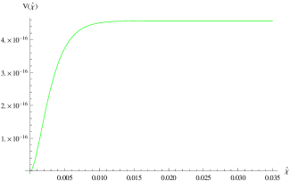
Figure 4: The inflationary potential $V(\hat{\chi})$ vs the inflaton-shift $\hat{\chi}$ for the benchmark model ${\cal B}_{1}$ while keeping the heavier moduli at their respective minima $\overline{\cal V},~{}\overline{\tau}_{s}$. The flat region of the potential is the relevant inflationary region where slow-roll conditions are satisfied.

Sufficient conditions for realizing slow-roll inflation are encoded in two so-called slow-roll parameters defined as

$$\begin{split}\epsilon(\chi)\equiv\frac{(\partial_{\chi}V_{\rm inf})^{2}}{2V_{\rm inf}^{2}}\,,\,\,\qquad\eta(\chi)\equiv\frac{\partial^{2}_{\chi}V_{\rm inf}}{V_{\rm inf}}\,.\end{split}$$ (38)

For slow-roll inflation to occur, one needs $\epsilon\ll 1\,,\,\eta\ll 1$ in a region of the moduli space. Our inflationary potential (LABEL:eq:Vinfnew) results in the following slow-roll parameters

$$\begin{split}&\epsilon(\chi)=\frac{8a_{w}^{4}\,\overline{\cal V}^{\frac{8}{3}}\,\chi^{\frac{2}{3}}\bigl{(}\chi^{\frac{4}{3}}-\overline{\chi}^{\frac{4}{3}}\bigr{)}^{2}}{9{\lambda_{sw}}^{2}\biggl{[}{\lambda_{sw}}-{\lambda_{sw}}\exp\Bigl{(}{\frac{a_{w}\overline{\cal V}^{\frac{2}{3}}\,(\chi^{\frac{4}{3}}-\overline{\chi}^{\frac{4}{3}})}{{\lambda_{sw}}}}\Bigr{)}+a_{w}\overline{\cal V}^{\frac{2}{3}}\,(\chi^{\frac{4}{3}}-\overline{\chi}^{\frac{4}{3}})\biggr{]}^{2}}\,,\\[5.69046pt] &\eta(\chi)=\frac{4a_{w}^{2}\,\overline{\cal V}^{\frac{4}{3}}\Bigl{(}4a_{w}\overline{\cal V}^{\frac{2}{3}}\chi^{\frac{4}{3}}(\chi^{\frac{4}{3}}-{\overline{\chi}}^{\frac{4}{3}})+{\lambda_{sw}}(-5\chi^{\frac{4}{3}}+{\overline{\chi}}^{\frac{4}{3}})\Bigr{)}}{9{\lambda_{sw}}^{2}\chi^{\frac{2}{3}}\biggl{(}{\lambda_{sw}}-{\lambda_{sw}}\exp\Bigl{(}\frac{a_{w}\overline{\cal V}^{\frac{2}{3}}\,(\chi^{\frac{4}{3}}-{\overline{\chi}}^{\frac{4}{3}})}{{\lambda_{sw}}}\Bigr{)}+a_{w}\overline{\cal V}^{\frac{2}{3}}\,(\chi^{\frac{4}{3}}-{\overline{\chi}}^{\frac{4}{3}})\biggr{)}}\,.\end{split}$$ (39)

These expressions contain exponentially suppressed large volume contributions and hence there is a good chance to satisfy the slow-roll conditions. For appropriate shift of the inflaton from its minimum, we indeed find slow-roll parameters satisfying $\epsilon\ll|\eta|\ll 1$. The process of inflation starts from a point $\chi^{\rm in}$ where $\epsilon\ll 1$, i.e. in a region where the potential is sufficiently flat. This period of inflation comes to an end at a point $\chi^{\rm end}$ where the slow-roll parameter becomes $\epsilon\sim{\cal O}(1)$. Figure 5 shows the variation of slow-roll parameters w.r.t. the inflaton shift.

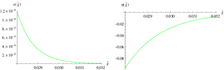
Figure 5: For benchmark model ${\cal B}_{1}$, the two slow-roll parameters $\epsilon(\hat{\chi})$ and $\eta(\hat{\chi})$ are displayed for inflaton shift $\hat{\chi}$ focussing on locating the slow-roll regime where $\epsilon\ll|\eta|\ll 1$.

Numerical fitting and estimates of cosmological parameters

Next, for several cosmological parameters, we compare the numerical estimates for our model with the experimental values extracted from the data of the WMAP experiment measuring the temperature fluctuations of the cosmological microwave background (CMB). Let us start with one of the central cosmological observables, the number of e-foldings during inflation. This can be computed as

$$\begin{split}N_{e}&\equiv\int_{\hat{\chi}^{\rm end}}^{\hat{\chi}^{\rm*}}\frac{V_{\rm inf}}{(\partial_{\chi}V_{\rm inf})}\,d\hat{\chi}\\ &\sim 3{\lambda_{sw}}\int_{\hat{\chi}^{\rm end}}^{\hat{\chi}^{\rm*}}\frac{\Bigl{(}-1+{\lambda_{sw}}\exp\Bigl{(}{\frac{a_{w}\overline{\cal V}^{\frac{2}{3}}\,(\chi^{\frac{4}{3}}-{\overline{\chi}}^{\frac{4}{3}})}{{\lambda_{sw}}}}\Bigr{)}\Bigr{)}+a_{w}\overline{\cal V}^{\frac{2}{3}}(-\chi^{\frac{4}{3}}+{\overline{\chi}}^{\frac{4}{3}})}{4a_{w}^{2}\,\overline{\cal V}^{\frac{4}{3}}\,\chi^{\frac{1}{3}}\,(\chi^{\frac{4}{3}}-{\overline{\chi}}^{\frac{4}{3}})}\,,\end{split}$$ (40)

where $\hat{\chi}^{\rm*}$ is the inflaton shift at the horizon exit and ${\hat{\chi}^{\rm end}}$ the inflaton shift corresponding to a slow-roll parameter $\epsilon=1$. For consistency with the observational data, the above expression for the number of e-foldings has to be of order $60$. Moreover, in the large volume limit, we have the following relation

$$\begin{split}\epsilon\ll|\eta|\sim\frac{1}{N_{e}}\,.\end{split}$$ (41)

The other cosmological observables of interest are the amplitudes and spectral indices for scalar and tensor perturbations. These are given (in $M_{\rm pl}=1$ units) as

$$\begin{split}&A_{S}=\frac{H}{2\sqrt{2}\,\pi\sqrt{\epsilon}}\sim 5\times 10^{-5}\,\,\,{{\rm(\,imposed\,\,by\,\,COBE\,\,observations)}}\,,\\ &n_{S}=1+2\eta-6\epsilon\,,\qquad\frac{dn_{S}}{d\ln k}=16\epsilon\eta-24\epsilon^{2}\,\,,\\ &A_{T}=\frac{\sqrt{2}H}{\pi}\,,\quad n_{T}=-2\epsilon\quad\text{and}\quad r\sim 12.4\epsilon\;.\end{split}$$ (42)

Here, $A_{S},~{}A_{T}$ are amplitudes of scalar and tensor perturbations and $n_{S},~{}n_{T}$ are their respective spectral indices. Furthermore, $r$ is the tensor-to-scalar ratio, for which values $r>0.1$ can be tested by the Planck satellite.

The dynamics of the inflaton modulus $\chi$ as well as the Hubble parameter $H$ is governed by the Friedman-equations (in units $M_{\rm pl}=1$)

$$\begin{split}&\frac{d^{2}\chi}{dt^{2}}+3H\frac{d\chi}{dt}+\partial_{\chi}V_{\rm inf}=0\,,\\ &H^{2}=\frac{1}{6}\left[2V_{\rm inf}+\left(\frac{d\chi}{dt}\right)^{2}\right]\,.\end{split}$$ (43)

In the slow-roll approximation, the Hubble parameter $H$ is such that $3H^{2}=V_{\rm inf}$. Matching the COBE normalization for the density fluctuations $\delta_{H}=1.92\times 10^{-5}$, results in a constraint defined in terms of a new parameter given as,

$$\begin{split}{\cal A}_{\rm COBE}\equiv\left(\frac{g_{s}}{8\pi}\right)\,e^{K_{\rm CS}}\left(\frac{V_{\rm inf}^{3}}{(\partial_{\chi}V_{\rm inf})^{2}}\right)\sim 2.7\times 10^{-7}\,.\end{split}$$ (44)

Further, the scale of inflation can be estimated as

$$\begin{split}M_{\rm inf}=V_{\rm inf}^{\frac{1}{4}}\,.\end{split}$$ (45)

As, in the slow-roll regime, the inflationary potential is flat by definition, the Hubble parameter and the scale of inflation (as defined above) do not vary significantly during the entire inflationary process. This is also reflected in figure 4.

Now, we present the numerical estimates for these cosmological data for the benchmark models ${\cal B}_{1}-{\cal B}_{4}$ in the tables 4 and 5. Also, in the figures 6 and 7, we show the dependence of $A_{\rm COBE}$ and $n_{S}$ on the value of the inflaton field.

	$\hat{\chi}^{\rm end}$	$\hat{\chi}^{*}$	$\epsilon$	$\eta$	$N_{e}$	$M_{\rm inf}({\rm GeV})$
${\cal B}_{1}$	$1.29\times 10^{-2}$	$3.08\times 10^{-2}$	$3.2\times 10^{-10}$	$-0.01644$	$60.84$	$3.5\times 10^{14}$
${\cal B}_{2}$	$1.26\times 10^{-2}$	$3.00\times 10^{-2}$	$2.9\times 10^{-10}$	$-0.01607$	$62.21$	$3.2\times 10^{14}$
${\cal B}_{3}$	$1.24\times 10^{-2}$	$2.95\times 10^{-2}$	$2.6\times 10^{-10}$	$-0.01544$	$64.79$	$3.0\times 10^{14}$
${\cal B}_{4}$	$1.22\times 10^{-2}$	$2.90\times 10^{-2}$	$2.4\times 10^{-10}$	$-0.01532$	$65.27$	$2.2\times 10^{14}$

Table 4: The numerical estimates for various cosmological observables -I.

	$n_{S}$	${\cal A}_{\rm COBE}$	$r$	$M_{\tau_{s}}$	$M_{\cal V}$	$M_{\tau_{w}}$
					($\times 10^{14}$ GeV)
${\cal B}_{1}$	0.9671	$7.1\times 10^{-7}$	$4.0\times 10^{-9}$	$297$	$3.49$	$0.28$
${\cal B}_{2}$	0.9679	$5.4\times 10^{-7}$	$3.6\times 10^{-9}$	$201$	$1.48$	$0.19$
${\cal B}_{3}$	0.9691	$4.7\times 10^{-7}$	$3.2\times 10^{-9}$	$214$	$1.23$	$0.12$
${\cal B}_{4}$	0.9694	$1.5\times 10^{-7}$	$3.0\times 10^{-9}$	$120$	$0.52$	$0.03$

Table 5: The numerical estimates for various cosmological observables -II.

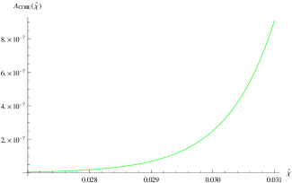
Figure 6: The dependence of $A_{\rm COBE}$ on the inflaton shift $\hat{\chi}$ (for model ${\cal B}_{1}$).

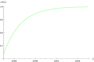
Figure 7: The dependence of the spectral index $n_{S}$ on the inflaton shift $\hat{\chi}$ (for model ${\cal B}_{1}$).

Note that, for benchmark model ${\cal B}_{1}$, the Hubble parameter during the inflationary epoch takes the value

$$\begin{split}H^{2}=-\frac{g_{s}e^{K_{\rm CS}}}{8\pi}\left(\frac{\mu_{2}\,e^{-a_{w}\overline{\tau}_{w}}}{a_{w}}\right)\sim 10^{-16}\end{split}$$ (46)

and therefore consistently reproduces the correct order of magnitude for the scalar power spectrum ${\cal P}_{S}=|A_{S}|^{2}=H^{2}/(8\pi^{2}\epsilon)$ with the slow-roll parameter $\epsilon$ being of order $10^{-10}$. Moreover, the masses of the moduli $\tau_{s},{\cal V}$ are larger than the value of the Hubble parameter ($H\sim 10^{10}$GeV) along the entire inflationary trajectory such that $M_{\tau_{s}}>M_{\cal V}>H\sim M_{\tau_{w}}$ and therefore, the heavier moduli remain at their respective minimum during the motion of the lightest (inflaton) modulus. Thus, our assumption of single field inflation is justified.

Let us close our numerical analysis with some general comments on this inflationary scenario.

• Since the form of the inflationary potential is exponentially flattened by the appearance of the large volume $\overline{\cal V}$ factor, the respective cosmological observables are extremely sensitive to the inflaton shift.

• All four benchmark models predict a negligible value of tensor-to-scalar ratio $r\sim 10^{-9}$ along with negligible values for other tensor mode parameters $n_{T},~{}A_{T}$. This is something very common in inflationary large volume models based on a blow-up modulus as inflaton field [21].

• Due to one of the inflationary slow-roll parameter being very small ($\epsilon\sim 10^{-10}$), the running of the scalar spectral index $\frac{dn_{S}}{d\ln k}$ is negligible.

• An equivalent convenient reformulation of the COBE normalization of density perturbations $\delta_{H}=1.92\times 10^{-5}$ is given as [21]

  $$\begin{split}\left(\frac{V_{\rm inf}}{\epsilon}\right)^{\frac{1}{4}}=6.6\times 10^{16}\,\,{\rm GeV}\,.\end{split}$$ (47)

  For instance, for benchmark model ${\cal B}_{1}$ we get $8\times 10^{16}$ GeV. This estimate is directly related to the scale of inflation, which comes out as $M_{\rm inf}\sim 10^{14}\,{\rm GeV}$. Therefore, our model belongs to the class of high scale inflationary models.

Reheating

Without going into too much detail of the post-inflationary processes, let us comment on the reheating of the universe at the end of inflation. Due to possible couplings of the inflaton to both observable and hidden sectors, its energy will be dumped into various channels. Further, as argued in [41], a mass gap can be generated via a dynamically generated scale $\Lambda$ appearing from the gaugino condensation in the field theroy supported on divisor $D_{s}$ which subsequently can make the hidden sector degrees of freedoms massive; to be more specific, the inflaton mass for our case is lighter as $M_{\rm inf}\sim\frac{M_{p}}{{\cal V}^{1+\frac{p}{2}}}<\Lambda\sim\frac{Mp}{{\cal V}^{5/6}}$ where $p>1$. Hence, similar to [36], the decay of the inflaton into this hidden sector particles is kinematically forbidden.

In order for the reheating process not to interfere with the hot big bang scenario and its successful description of nucleosynthesis, it is important to determine the reheating temperature $T_{\rm rh}$. This can be computed from the decay width of the inflation into the various allowed observable channels. For this purpose, one has to compute the couplings of the inflaton to the Standard Model gauge and matter fields.

For the string inspired model of interest one proceeds as follows [42]. Expanding the divisor volume moduli around their respective minima as $\tau_{i}=\overline{\tau}_{i}+\delta\tau_{i}$, one arrives at the following form of a generic Lagrangian,

$$\begin{split}{\cal L}=\sum_{ij}K_{ij}(\partial_{\mu}\delta\tau_{i})(\partial^{\mu}\delta\tau_{j})-\langle V\rangle-\frac{1}{2}\sum_{ij}V_{ij}\,\delta\tau_{i}\,\delta\tau_{j}+{\cal O}(\delta\tau^{3})\,.\end{split}$$ (48)

Let us denote by $C_{ai}$ and $(M^{2})_{a}$ the eigenvectors and eigenvalues of the matrix ${\cal M}_{ij}=\frac{1}{2}(K^{-1}\,V)_{ij}$. Choosing the normalization $C^{T}_{a}\,K\,C_{b}=\delta_{ab}$ and redefining $\delta\tau_{i}=\frac{1}{\sqrt{2}}C_{ai}\delta\phi_{a}$, the Lagrangian (48) becomes

$$\begin{split}\ {\cal L}=\frac{1}{2}\sum_{a}(\partial_{\mu}\delta\phi_{a})(\partial^{\mu}\delta\phi_{a})-\langle V\rangle-{\frac{1}{2}}\sum_{a}M_{a}^{2}\,\delta\phi_{a}^{2}\,,\end{split}$$ (49)

so that the $\delta\phi_{a}$ constitute a canonical normalized basis. The details of this computation for our model are collected in appendix D.

As we have not supported any (MS)SM-like model explicitly in the current setup, we just focus on the inflaton coupling to two light gauge-bosons living on a D7-brane worldvolume. In a complete realistic model, the decay channels of the moduli into matter fields have to be analyzed, as well. The relevant coupling arises from the gauge kinetic function and gives the three-point coupling

$$\begin{split}{\cal L}_{\rm gauge}=-\tau_{i}\,F_{\mu\nu}^{(i)}\,F^{\mu\nu}_{(i)}\,.\end{split}$$ (50)

At the end of inflation, the inflaton oscillates around its minimum value so that, expanding $\tau_{i}=\delta\tau_{i}+\overline{\tau}_{i}$, one gets the couplings

$${\cal L}_{\rm gauge}=-\frac{1}{4}G_{\mu\nu}^{(i)}\,G^{\mu\nu}_{(i)}-\frac{\delta\tau_{i}}{4\overline{\tau}_{i}}\,G_{\mu\nu}^{(i)}\,G^{\mu\nu}_{(i)}$$ (51)

for the canonically normalized field $G_{\mu\nu}^{(i)}=2F_{\mu\nu}^{(i)}\sqrt{\overline{\tau}_{i}}$. As argued earlier, we can write $\delta\tau_{i}$ in terms of fluctuations of canonically normalized field as given in appendix D.

To proceed, we assume now that the observable sector is localized on a stack of $D7$-branes wrapping the small divisor $D_{s}$. The numerical estimates for appropriate normalization for the corresponding divisor volume modulus fluctuation $\delta\tau_{s}$ which is relevant for the current purpose can be read from the appendix D. For instance, the expression for benckmark model ${\cal B}_{1}$ from (D) is,

$$\delta{\tau_{s}}=-0.258\,\,\delta\chi_{1}-28.736\,\,\delta\chi_{2}-0.0168\,\,\delta\chi_{3}\,.$$

From above equation, one can read the volume scaling of the coupling of the inflaton $\chi_{3}$ to two gauge bosons as $g_{\gamma\gamma\chi_{3}}\sim{0.0168}/({4\bar{\tau}_{s}})=7.39\times 10^{-4}\,\,M_{p}^{-1}$. Hence, using $M_{\chi_{3}}=1.19\times 10^{-5}\,\,M_{p}$, the decay width of the channel $\chi_{3}\longrightarrow\{\gamma,\gamma\}$ is estimated from

$$\begin{split}\Gamma_{\chi_{3}\rightarrow\{\gamma,\gamma\}}=\frac{N_{g}\,g_{\chi_{3}\gamma\gamma}^{2}\,M_{\chi_{3}}^{3}}{64\pi}\end{split}$$ (52)

Here, $N_{g}$ denotes the total number of gauge bosons (e.g. in MSSM it is 12) and subsequently, an estimated reheating temperature is simply given as

$$\begin{split}T_{\rm rh}\sim\sqrt{\Gamma M_{\rm pl}}\,.\end{split}$$ (53)

which comes out to be $1.8\times 10^{7}\,\,{\rm GeV}$ for our benchmark models ${\cal B}_{1}$. In fact in all our benchmark models, the reheating temperature estimated via the aforementioend computations turns out to be $T_{\rm rh}\sim(10^{6}-10^{7})\,{\rm GeV}$ which is much higher than the big bang nucleosynthesis temperature $T_{\rm BBN}\simeq 1$ MeV.

Loop corrections

Since the dynamics of the inflaton field is ruled by a non-perturbative contribution to the superpotential, one must be worried about more relevant corrections, i.e. in particular string loop corrections to the Kähler potential. Here one can distinguish between open and closed string loop corrections, i.e. annulus and torus diagrams. For moduli stabilization in the LARGE volume scenario, the open string corrections have been shown to exhibit an extended no-scale structure [47] implying that their contributions to the scalar potential are sub-dominant against the standard LARGE volume potential.

However, for inflation such corrections potentially induce an $\eta$-problem, i.e. that, if the inflaton moves far away from its minimum during inflation, loop-effects might be strong enough to spoil the flatness of the potential [23, 45]. Hence, similar to the case of blow-up inflation loop-effects might be crucial for our case, as well.

What the effective theory on the tadpole canceling $D7$-brane configuration is concerned, our model is clearly way too simple. In fact, we only have a single stack of $D7$-branes right on top of the $O7$-plane. These do wrap the small cycle, whose volume modulus is $\tau_{s}$. Therefore, according to [47], the only open string loop corrections come from Kaluza-Klein mode exchange and are conjectured to lead to a contribution to the Kähler potential of the form

$$\begin{split}\Delta K=\frac{\sqrt{\tau_{s}}\,{\cal E}(U,\overline{U})}{{\cal V}\,{\rm Im}(\tau)}\,.\end{split}$$ (54)

Moreover, since the natural cut-off scale of the effective four-dimensional theory is $\Lambda=1/{\cal V}^{\frac{1}{6}}$, we expect the closed string loop correction to only depend on the overall volume modulus ${\cal V}$. Therefore, the loop corrections do not explicitly depend on the inflaton $\tau_{w}$ (respectively the canonically normalized field $\chi_{3}$) so that, at least for this very simple model, we do not expect an $\eta$-problem to be generated by loop-effects.

5 Conclusions

In this article, we presented a new class of Kähler moduli inflation models realized in the LARGE volume scenario in the context of Type IIB orientifold compactifications. For prior work in this framework one could distinguish essentially two different classes of Kähler moduli inflationary models, blow-up inflation [21] and fiber inflation [23, 36]. The first kind starts with a standard LARGE volume scenario and considers one of the blow-up modes as the inflaton, whose leading order contribution to the scalar potential arises from a non-perturbative instanton correction to the superpotential. For the second class, the starting point is a Calabi-Yau threefold which is $K3$-fibered and also contains shrinkable del Pezzo divisors. The inflaton is given by the size modulus of the $K3$ fiber and the potential can be generated either by loop [23] or by poly-instanton effects [36].

The model considered in this paper is different but shares some of the features of both blow-up and fiber inflation. The inflaton is neither a blow-up mode nor a fiber mode but actually a Kähler modulus corresponding to a so-called Wilson line divisor, which can be realized as a $\mathbb{P}^{1}$ fibration over $\mathbb{T}^{2}$. Like in fiber inflation, the leading order contribution to the inflationary scalar potential arises from sub-leading (poly-instanton) corrections to the superpotential, however, the contribution of the inflaton to the Calabi-Yau volume form and therefore to the Kähler potential is very similar to a blow-up mode.

As a prerequisite for inflation, in a simple representative model with three Kähler moduli, we first studied the issue of moduli stabilization. We considered two schemes. The minimal setup contained just the leading order ${\alpha^{\prime}}$-correction to the Kähler potential as well as a non-perturbative ($E3$ and poly-instanton) contribution to the superpotential. Our conclusion was that it is not possible to stabilize all the moduli within the geometric regime. In the second extended scheme this could be improved by starting with a racetrack form of the non-perturbative superpotential. Since this ansatz contains more parameters, all moduli were stabilized inside the geometric regime of the Kähler cone.

After identifying four benchmark models, we explored the possibility that the volume of Wilson-line divisor can play the role of an inflaton field. Being in a setup equipped with a swiss-cheese like volume form and poly-instanton effects, the inflationary signatures of the model are expected to be a hybrid of the blow-up and fiber-inflation models, i.e. one expects to see features from both inflationary scenarios. Indeed, the intermediate steps in moduli stabilization process and the form of inflationary potential as a function of the divisor volume moduli look quite similar to those of [36]. However, as the field redefinitions related to canonical normalization of kinetic terms are similar to those of the moduli involved in blow-up inflationary models, the expressions for slow-roll parameters and other cosmological observables turn out to be rather similar to the blow-up case.

Due to the appearing exponential suppression factors in the large volume regime, the slow-roll conditions are easily satisfied. Moreover, for certain choices of the initial parameters one can bring the number of e-foldings, the density perturbation amplitude and the spectral index in perfect agreement with the current observational constraints. The model predicts a negligible value for the parameters involving tensor perturbation modes, like the tensor-to-scalar ratio $r$, the spectral index $n_{T}$ and the amplitude $A_{T}$. The inflaton rolls over sub-Planckian distances so that the model belongs to the class of ‘small’ field inflation. Furthermore, the scale of inflation could be shown to be quite high (of the order $10^{14}$GeV), which means that we are dealing with a ‘high’ scale inflationary model.

Contrary to blow-up inflationary models, the stabilized value of the Calabi-Yau volume turns out to be relatively low (${\cal V}\sim{\cal O}(10^{3})$) for generating sufficient amount of scalar perturbation along with ${\cal O}(60)$ number of e-foldings. At the end of inflation, the decay of the inflaton into the degrees of freedom of a (toy) visible sector cause a reheating temperature of the order $T_{\rm rh}\sim(10^{6}-10^{7})$GeV which is much larger than the lower bound given by the big bang nucleosynthesis temperature $T_{\rm BBN}\sim{\rm MeV}$. However, addressing this issue needs more attention in a less simple setup as compared to ours where one could explicitly distinguish the hidden and visible sectors to get the relevant couplings for estimating all decay channels. In such cases, there might be a possibility of inflaton dumping most of its energy to the hidden sector instead of visible sector.

In this paper we have only analyzed the most simple conceivable set-up for having a poly-instanton generated contribution to the superpotential. Due to the small number of involved Kähler moduli, this clearly does not admit enough freedom to also support a realistic (MS)SM on intersecting, fluxed $D7$-branes. For a more thorough analysis of the interactions between the inflaton sector and the visible sector and of possibly dangerous loop-corrections an extension of our model in this direction is necessary.

Acknowledgments

We would like to thank Michele Cicoli, Shanta de Alwis, Sebastian Halter, Stefan Hohenegger, Dieter Lüst, Pablo Soler, Zhongliang Tuo and Angel Uranga for helpful discussions. RB is grateful to the Simons Center for Physics and Geometry at Stony Brook University for hospitality. XG is supported by the MPG-CAS Joint Doctoral Promotion Programme. PS is supported by a postdoctoral research fellowship from the Alexander von Humboldt Foundation.

Appendix A Kähler metric and its inverse

The Kähler potential is given as $K=-2\,\ln{\cal Y}$, where ${\cal Y}\equiv{\cal V}+C_{\alpha^{\prime}}$ is defined in terms of Kähler coordinates as

$$\begin{split}{\cal Y}=\xi_{b}(T_{b}+\bar{T}_{b})^{\frac{3}{2}}-\xi_{s}(T_{s}+\bar{T}_{s})^{\frac{3}{2}}-\xi_{sw}\Bigl{(}(T_{s}+\bar{T}_{s})+(T_{w}+\bar{T}_{w})\Bigr{)}^{\frac{3}{2}}+C_{\alpha^{\prime}}\,,\end{split}$$ (55)

and the perturbative ${\alpha^{\prime}}^{3}$ contribution is being given as $C_{\alpha^{\prime}}=-\frac{\chi(CY_{3})\,({{\tau}-\bar{\tau}})^{\frac{3}{2}}\zeta[3]}{4(2\pi)^{3}\,({2i})^{\frac{3}{2}}}$. The expression of Kähler derivative can be read as

$$\partial_{T_{b}}K=-\frac{3\sqrt{2}\,\xi_{b}\,\sqrt{\tau_{b}}}{{\cal Y}}\,\,,$$ (56)

$$\partial_{T_{s}}K=\frac{3\sqrt{2}\,(\xi_{s}\,\sqrt{\tau_{s}}+\xi_{sw}\,\sqrt{\tau_{s}+\tau_{w}})}{{\cal Y}}\,\,,$$

$$\partial_{T_{w}}K=\frac{3\sqrt{2}\,\xi_{sw}\,\sqrt{\tau_{s}+\tau_{w}}}{{\cal Y}}\,.$$

The expressions for the various components of the Kähler metric are given as under,

$$K_{T_{b}{\bar{T}}_{b}}=-\frac{{3\sqrt{2}\xi_{b}\,{\cal Y}}-36\xi_{b}^{2}{\tau_{b}}^{3/2}}{4\,{\cal Y}^{2}\,{\sqrt{{\tau_{b}}}}}\,\,,$$

$$K_{T_{b}{\bar{T}}_{s}}=-\frac{9\xi_{b}\sqrt{{\tau_{b}}}\left(\sqrt{{\tau_{s}}}\xi_{s}+\xi_{sw}\sqrt{{\tau_{s}}+{\tau_{w}}}\right)}{\,{\cal Y}^{2}}=K_{T_{s}{\bar{T}}_{b}}\,,$$

$$K_{T_{b}{\bar{T}}_{w}}=-\frac{9\xi_{b}\,\xi_{sw}\sqrt{{\tau_{b}}}\sqrt{{\tau_{s}}+{\tau_{w}}}}{\,{\cal Y}^{2}}=K_{T_{w}{\bar{T}}_{b}}\,,$$ (57)

$$K_{T_{s}{\bar{T}}_{s}}=\frac{3\left(\sqrt{2}{\cal Y}\,\left(\frac{\xi_{s}}{\sqrt{{\tau_{s}}}}+\frac{\xi_{sw}}{\sqrt{{\tau_{s}}+{\tau_{w}}}}\right)+12\left(\xi_{s}\sqrt{\tau}_{s}+\xi_{sw}\sqrt{\tau_{s}+\tau_{w}}\right)^{2}\right)}{4\,{\cal Y}^{2}}\,,$$

$$K_{T_{s}{\bar{T}}_{w}}=\frac{3\xi_{sw}\left(\sqrt{2}{\cal Y}+12(\tau_{s}+\tau_{w})\left(\xi_{s}\sqrt{\tau}_{s}+\xi_{sw}{\sqrt{\tau_{s}+\tau_{w}}}\right)\right)}{4\,{\cal Y}^{2}\sqrt{{\tau_{s}}+{\tau_{w}}}}=K_{T_{w}{\bar{T}}_{s}}\,,$$

$$K_{T_{w}{\bar{T}}_{w}}=\frac{3\xi_{sw}(\sqrt{2}{\cal Y}+12\xi_{sw}({{\tau_{s}}+{\tau_{w}}})^{3/2})}{4\,{\cal Y}^{2}\sqrt{{\tau_{s}}+{\tau_{w}}}}\,.$$

The expressions for various components of the inverse Kähler metric are given as under,

$$K^{T_{b}{\bar{T}}_{b}}=-\frac{2\sqrt{2}\,{\cal Y}\,\sqrt{\tau}_{b}}{3\xi_{b}}+\frac{8{\cal Y}\,\tau_{b}^{2}}{{\cal Y}-3{\cal V}}\,\,,\,\,K^{T_{b}{\bar{T}}_{i}}=-\frac{8{\cal Y}\,\tau_{b}\,\tau_{i}}{{\cal Y}-3{\cal V}}=K^{T_{i}{\bar{T}}_{b}},\,\{i=s,w\},$$ (58)

$$K^{T_{s}{\bar{T}}_{s}}=\frac{2\sqrt{2}\,{\cal Y}\,\sqrt{\tau}_{s}}{3\xi_{s}}-\frac{8{\cal Y}\,\tau_{s}^{2}}{{\cal Y}-3{\cal V}}\,,\,K^{T_{s}{\bar{T}}_{w}}=-\frac{2\sqrt{2}\,{\cal Y}\,\sqrt{\tau}_{s}}{3\xi_{s}}-\frac{8{\cal Y}\,\tau_{s}\tau_{w}}{{\cal Y}-3{\cal V}}=K^{T_{w}{\bar{T}}_{s}}\,,$$

$$K^{T_{w}{\bar{T}}_{w}}=\frac{2\sqrt{2}\,{\cal Y}\,{\sqrt{\tau_{s}+\tau_{w}}}}{3\xi_{sw}}-\frac{8{\cal Y}\,\tau_{w}^{2}}{{\cal Y}-3{\cal V}}+\frac{2\sqrt{2}\,{\cal Y}\,{\sqrt{\tau_{s}}}}{3\xi_{s}}\,,$$

where in terms of divisor volumes $\tau_{i}$’s, we have

$$\begin{split}{\cal Y}\equiv{\cal V}+C_{\alpha^{\prime}}=2\sqrt{2}\left(\xi_{b}\,\tau_{b}^{3/2}-\xi_{s}\,\tau_{s}^{3/2}-\xi_{sw}\,(\tau_{s}+\tau_{w})^{3/2}\right)+C_{\alpha^{\prime}}\,.\end{split}$$ (59)

The above form of the Kähler metric and its inverse are exact for the given ansatz of Kähler potential. After neglecting the $\alpha^{\prime}$-corrections in the large volume limit (i.e. using ${\cal Y}\sim{\cal V}\sim 2\sqrt{2}\,\xi_{b}\,\tau_{b}^{3/2}$), this simplifies to the form

$$\hskip-28.45274ptK^{A\bar{B}}\sim\left(\begin{array}[]{lll}\frac{4\tau_{b}^{2}}{3}&4\tau_{b}\tau_{s}&4\tau_{b}\tau_{w}\\ 4\tau_{b}\tau_{s}&\frac{8\xi_{b}\,\tau_{b}^{3/2}\,\sqrt{\tau}_{s}}{3\,\xi_{s}}&-\frac{8\xi_{b}\,\tau_{b}^{3/2}\,\sqrt{\tau}_{s}}{3\,\xi_{b}}\\ 4\tau_{b}\tau_{w}&-\frac{8\xi_{b}\,\tau_{b}^{3/2}\,\sqrt{\tau}_{s}}{3\,\xi_{s}}&\frac{8\xi_{b}\,\tau_{b}^{3/2}\,(\xi_{s}{\sqrt{\tau_{s}+\tau_{w}}}+\xi_{sw}\sqrt{\tau}_{s})}{3\,\xi_{s}\,\xi_{sw}}\end{array}\right)\,.$$ (63)

The above form reflects the strong swiss-cheese nature of the volume form for the $\{T_{b},T_{s}\}$ moduli sector, while the $T_{w}$ modulus makes a (slight) difference.

Appendix B The F-term scalar potential

From the generic expressions of the Kähler potential $K$ and the superpotential $W$, one can compute the scalar potential from (10).

Scheme 1: minimal

After collecting the most dominant contributions of three types of terms, the generic expression of the F-term scalar potential is given as

$$\begin{split}V(\tau_{b},\tau_{s},\tau_{w},\rho_{s},\rho_{w})\equiv V({\cal V},\tau_{s},\tau_{w},\rho_{s},\rho_{w})=V_{\alpha^{\prime}}+V_{\rm np1}+V_{\rm np2}\,,\end{split}$$ (64)

where

$$V_{\alpha^{\prime}}=\frac{3{\,{\cal C}_{\alpha^{\prime}}}\,|W_{0}|^{2}}{2{\cal V}^{3}}\,,$$

$$V_{\rm np1}=\frac{4\,{W_{0}}}{{\cal V}^{2}}\biggl{[}{\,{A_{s}}}\,e^{-{a_{s}\tau_{s}}-{a_{w}\,\tau_{w}}}\biggl{\{}{\,a_{s}}e^{{a_{w}\,\tau_{w}}}{\tau_{s}}\cos({\,a_{s}}{\rho_{s}})$$ (65)

$$\hskip 122.85876pt+{\,{A_{w}}}({a_{s}\tau_{s}}+{a_{w}\,\tau_{w}})\cos({\,a_{s}}{\rho_{s}}+{\,{a_{w}}}{\rho_{w}})\biggr{\}}\biggr{]}\,,$$

$$V_{\rm np2}=\frac{2\sqrt{2}}{3\,\xi_{s}\,\xi_{sw}\,{\cal V}}\biggl{[}{\,{A_{s}}}^{2}e^{-2({a_{s}\tau_{s}}+{a_{w}\,\tau_{w}})}\biggl{(}\xi_{sw}\left({\,{A_{w}}}^{2}+e^{2{a_{w}\,\tau_{w}}}\right)\sqrt{{\tau_{s}}}{\,a_{s}}^{2}$$

$$\hskip 28.45274pt+2({\,a_{s}}-{\,{a_{w}}}){\,{A_{w}}}\xi_{sw}\,e^{{a_{w}\,\tau_{w}}}\sqrt{{\tau_{s}}}\cos({\,{a_{w}}}{\rho_{w}}){\,a_{s}}-2{\,{a_{w}}}{\,{A_{w}}}^{2}\xi_{sw}\sqrt{{\tau_{s}}}{\,a_{s}}$$

$$\hskip 151.76744pt+{\,{a_{w}}}^{2}{\,{A_{w}}}^{2}\left(\sqrt{{\tau_{s}}+{\tau_{w}}}\xi_{s}+\xi_{sw}\sqrt{{\tau_{s}}}\right)\biggr{)}\biggr{]}\,.$$

Scheme 2: racetrack

After collecting the most dominant contributions of three types of terms, the generic expression of the F-term scalar potential with the racetrack superpotential, is given as

$${\bf V}(\tau_{b},\tau_{s},\tau_{w},\rho_{s},\rho_{w})\equiv{\bf V}({\cal V},\tau_{s},\tau_{w},\rho_{s},\rho_{w})={\bf V}_{\alpha^{\prime}}+{\bf V}_{\rm np1}+{\bf V}_{\rm np2}\,,$$ (66)

where

$$\hskip-19.91684pt{\bf V}_{\alpha^{\prime}}=\frac{3{\,{\cal C}_{\alpha^{\prime}}}\,|W_{0}|^{2}}{2\,{\cal V}^{3}}\,,$$

$$\hskip-19.91684pt{\bf V}_{\rm np1}=\frac{4\,{W_{0}}}{{\cal V}^{2}}\biggl{\{}\,a_{s}\,{A_{s}}e^{-\,a_{s}{\tau_{s}}}{\tau_{s}}\cos(\,a_{s}{\rho_{s}})-{\,b_{s}\,{B_{s}}e^{-\,b_{s}{\tau_{s}}}{\tau_{s}}\cos(\,b_{s}{\rho_{s}})}$$ (67)

$$\hskip 85.35826pt+{\,{A_{s}}\,{A_{w}}e^{-\,a_{s}{\tau_{s}}-{a_{w}}{\tau_{w}}}(a_{s}{\tau_{s}}+a_{w}\tau_{w})\cos(a_{s}{\rho_{s}}+{a_{w}}{\rho_{w}})}$$

$$\hskip 113.81102pt-{{B_{s}}\,{B_{w}}e^{-\,b_{s}{\tau_{s}}-{a_{w}}{\tau_{w}}}(b_{s}{\tau_{s}}+a_{w}\tau_{w})\cos(b_{s}{\rho_{s}}+{a_{w}}{\rho_{w}})}\biggr{\}}\,,$$

$$\hskip-19.91684pt{\bf V}_{\rm np2}=\frac{2\sqrt{2}\,\sqrt{{\tau_{s}}}}{3\xi_{s}\,{\cal V}}\biggl{\{}\,a_{s}^{2}\,{A_{s}}^{2}\,e^{-2\,a_{s}{\tau_{s}}}+{\,b_{s}^{2}\,{B_{s}}^{2}e^{-2\,b_{s}{\tau_{s}}}}-{2\,a_{s}\,b_{s}\,{A_{s}}\,{B_{s}}e^{-(\,a_{s}+\,b_{s}){\tau_{s}}}}$$

$$\hskip 14.22636pt\times\cos((\,a_{s}-\,b_{s}){\rho_{s}})\biggr{\}}+\frac{2\sqrt{2}e^{-2(a_{s}+b_{s}){\tau_{s}}}}{3\xi_{s}\,\xi_{sw}\,{\cal V}}\biggl{\{}e^{-2a_{w}{\tau_{w}}}\bigl{(}A_{s}^{2}a_{w}^{2}\xi_{s}e^{2b_{s}{\tau_{s}}}\sqrt{{\tau_{s}}+{\tau_{w}}}A_{w}^{2}$$

$$\hskip 14.22636pt+2\,{A_{s}}\,B_{s}e^{(a_{s}+b_{s}){\tau_{s}}}\bigl{(}-\,A_{w}\xi_{s}\,B_{w}\sqrt{{\tau_{s}}+{\tau_{w}}}a_{w}^{2}-a_{s}b_{s}\,\xi_{sw}e^{2a_{w}{\tau_{w}}}\sqrt{{\tau_{s}}}+(a_{s}-a_{w})$$

$$\hskip 14.22636pt\times\,A_{w}(a_{w}-b_{s})\,B_{w}\xi_{sw}\,\sqrt{{\tau_{s}}}\bigr{)}\cos((a_{s}-b_{s}){\rho_{s}})-2\xi_{sw}e^{a_{w}{\tau_{w}}}\sqrt{{\tau_{s}}}\bigl{(}\bigl{(}a_{s}(a_{w}-a_{s})\,$$

$$\hskip 14.22636pt\times A_{w}e^{2b_{s}{\tau_{s}}}\,{A_{s}}^{2}+(a_{w}-b_{s})b_{s}\,B_{s}^{2}\,B_{w}e^{2a_{s}{\tau_{s}}}\bigr{)}\cos(a_{w}{\rho_{w}})+\,{A_{s}}\,B_{s}e^{(a_{s}+b_{s}){\tau_{s}}}(a_{s}$$

$$\hskip 14.22636pt\times(b_{s}-a_{w})\,B_{w}\cos(a_{s}{\rho_{s}}-b_{s}{\rho_{s}}-a_{w}{\rho_{w}})+(a_{s}-a_{w})\,A_{w}b_{s}\cos(a_{s}{\rho_{s}}-b_{s}{\rho_{s}}$$

$$\hskip 14.22636pt+a_{w}{\rho_{w}}))\bigr{)}+\xi_{sw}e^{2a_{w}{\tau_{w}}}\bigl{(}a_{s}^{2}e^{2b_{s}{\tau_{s}}}\,{A_{s}}^{2}+b_{s}^{2}\,B_{s}^{2}e^{2a_{s}{\tau_{s}}}\bigr{)}\sqrt{{\tau_{s}}}+\xi_{sw}\bigl{(}\,{A_{s}}^{2}(a_{s}-a_{w})^{2}$$

$$\hskip 14.22636pt\times e^{2b_{s}{\tau_{s}}}\,A_{w}^{2}+(a_{w}-b_{s})^{2}\,B_{s}^{2}B_{w}^{2}e^{2a_{s}{\tau_{s}}}\bigr{)}\sqrt{{\tau_{s}}}+a_{w}^{2}b\,B_{s}^{2}\,B_{w}^{2}e^{2a_{s}{\tau_{s}}}\sqrt{{\tau_{s}}+{\tau_{w}}}\bigr{)}\biggr{\}}\,.$$

Appendix C Canonical normalization of Kähler moduli

The simplified Kähler metric after neglecting the $\alpha^{\prime}$-correction in the large volume limit is given as

$$K_{I\bar{J}}=\left(\begin{array}[]{lll}-\frac{\frac{3\sqrt{2}\xi_{b}\,{\cal V}}{\sqrt{{\tau_{b}}}}-36\xi_{b}^{2}{\tau_{b}}}{4\,{\cal V}^{2}}&-\frac{9\xi_{b}\sqrt{{\tau_{b}}}\left(\sqrt{{\tau_{s}}}\xi_{s}+\xi_{sw}\sqrt{{\tau_{s}}+{\tau_{w}}}\right)}{\,{\cal V}^{2}}&-\frac{9\xi_{b}\,\xi_{sw}\sqrt{{\tau_{b}}}\sqrt{{\tau_{s}}+{\tau_{w}}}}{\,{\cal V}^{2}}\\ -\frac{9\xi_{b}\sqrt{{\tau_{b}}}\left(\sqrt{{\tau_{s}}}\xi_{s}+\xi_{sw}\sqrt{{\tau_{s}}+{\tau_{w}}}\right)}{\,{\cal V}^{2}}&\frac{3\left(\frac{\xi_{s}}{\sqrt{{\tau_{s}}}}+\frac{\xi_{sw}}{\sqrt{{\tau_{s}}+{\tau_{w}}}}\right)}{2\sqrt{2}\,{\cal V}}&\frac{3\xi_{sw}}{2\sqrt{2}\,{\cal V}\sqrt{{\tau_{s}}+{\tau_{w}}}}\\ -\frac{9\xi_{b}\xi_{sw}\sqrt{{\tau_{b}}}\sqrt{{\tau_{s}}+{\tau_{w}}}}{\,{\cal V}^{2}}&\frac{3\xi_{sw}}{2\sqrt{2}\,{\cal V}\sqrt{{\tau_{s}}+{\tau_{w}}}}&\frac{3\xi_{sw}}{2\sqrt{2}\,{\cal V}\sqrt{{\tau_{s}}+{\tau_{w}}}}\end{array}\right)\,.$$

Utilizing the above Kähler metric, all kinetic terms for the respective moduli can be written as

$$\begin{split}{\cal L}_{\rm kinetic}({\cal V},\tau_{s},\tau_{w},\rho_{b},\rho_{s},\rho_{w})\equiv K_{I\bar{J}}(D_{\mu}T_{I})({\bar{D}}^{\mu}{\bar{T}}_{\bar{J}})=\frac{1}{2}\sum_{i=1}^{6}({\partial_{\mu}}{\chi_{i}})({\partial^{\mu}}{\chi_{i}})\,,\end{split}$$ (69)

where the summation is over six real moduli $\chi_{i}$ which constitute the canonically normalized forms of six real moduli $\{{\cal V},\tau_{s},\tau_{w},\rho_{b},\rho_{s},\rho_{w}\}$. Furthermore, as for the time being we are not interested in the dynamics of axion moduli, we consider the terms corresponding to the (divisor) volume modulus only. The leading and next-to-leading order kinetic terms for the volume moduli $\{{\cal V},\tau_{s},\tau_{w}\}$ can be easily read off as

$${\cal L}_{\rm kinetic}({\cal V},\tau_{s},\tau_{sw})\equiv\frac{1}{2}\sum_{i}^{3}({\partial_{\mu}}{\chi_{i}})({\partial^{\mu}}{\chi_{i}})=K_{1}+K_{2}+K_{3}+...\,,\,\,\,\,{\rm where}$$

$$K_{1}=\frac{1}{3{\cal V}^{2}}({\partial_{\mu}}{\cal V})^{2}\sim{\cal O}(1)\,,$$

$$K_{2}=\frac{3}{2\sqrt{2}{\cal V}}\left\{\frac{\xi_{s}({\partial_{\mu}}\tau_{s})^{2}}{\sqrt{\tau_{s}}}+\frac{\xi_{sw}({\partial_{\mu}}{\tau_{sw}})^{2}}{\sqrt{\tau_{sw}}}\right\}-\frac{\sqrt{2}}{{\cal V}}\left(\frac{{\partial_{\mu}}{\cal V}}{{\cal V}}\right)\biggl{\{}\xi_{s}{\sqrt{\tau}_{s}}({\partial_{\mu}}\tau_{s})$$

$$\hskip 28.45274pt+\xi_{sw}{\sqrt{\tau_{sw}}}({\partial_{\mu}}{\tau_{sw}})-\left(\frac{{\partial_{\mu}}{\cal V}}{{\cal V}}\right)(\xi_{s}\,\tau_{s}^{\frac{3}{2}}+\xi_{sw}\,{\tau_{sw}}^{\frac{3}{2}})\biggr{\}}\sim{\cal O}\left(\frac{1}{{\cal V}}\right)\,,$$

$$K_{3}=\frac{3\xi_{s}\xi_{sw}}{{\cal V}^{2}{\sqrt{\tau_{s}}}{\sqrt{\tau_{sw}}}}\left(\tau_{s}({\partial_{\mu}}{\tau_{sw}})-\tau_{sw}({\partial_{\mu}}{\tau_{s}})\right)^{2}\sim{\cal O}\left(\frac{1}{{\cal V}^{2}}\right)\,.$$ (70)

where $\tau_{sw}=\tau_{s}+\tau_{w}$. At the leading order, the overall Calabi-Yau volume $\cal V$ is canonically normalized from $K_{1}$ as

$$\begin{split}{\cal V}\sim\exp\left({\textstyle{\sqrt{\frac{3}{2}}}}\,\chi_{1}\right)\,.\end{split}$$ (71)

Utilizing the same, the sub-leading terms appearing as diagonal contributions to $\tau_{s}$ and ${\tau_{w}}$ result in canonically normalized forms given as

$$\hskip-19.91684pt\tau_{s}\sim\frac{1}{\lambda_{s}}\exp\left({\textstyle{\sqrt{\frac{2}{3}}}}\,\chi_{1}\right)\,\chi_{2}^{\frac{4}{3}}\,,\qquad{\tau_{s}+\tau_{w}}\sim\frac{1}{\lambda_{sw}}\exp\left({\textstyle{\sqrt{\frac{2}{3}}}}\,\chi_{1}\right)\,\chi_{3}^{\frac{4}{3}}\,,$$ (72)

where $\lambda_{s}=\frac{2^{\frac{7}{3}}\xi_{s}^{\frac{2}{3}}}{3^{\frac{2}{3}}}$ and $\lambda_{sw}=\frac{2^{\frac{7}{3}}\xi_{sw}^{\frac{2}{3}}}{3^{\frac{2}{3}}}$ are constants to be directly read off from the volume form. These aforementioned canonical forms of ${\cal V}$ and $\tau_{s},{\tau_{w}}$ receive corrections at sub-leading orders. Including ${\cal O}\left(\frac{1}{{\cal V}}\right)$ corrections, we have the following expressions of canonically normalized (divisor) volume moduli

$$\hskip-17.07182pt{\cal V}\sim\exp\left({\textstyle{{\sqrt{\frac{3}{2}}}}}\,\chi_{1}+{\textstyle\frac{3}{4}}\sum_{i=2}^{3}{\chi_{i}}^{2}\right)\,,$$

$$\hskip-17.07182pt\tau_{s}\sim\frac{1}{\lambda_{s}}\exp\left({\textstyle{\sqrt{\frac{2}{3}}}}\,\chi_{1}\right)\,\left(1+{\textstyle\frac{1}{2}}\sum_{i=2}^{3}{\chi_{i}}^{2}\right)\chi_{2}^{\frac{4}{3}}\,,$$ (73)

$$\hskip-17.07182pt\tau_{w}\sim\exp\left({\textstyle{\sqrt{\frac{2}{3}}}}\,\chi_{1}\right)\,\left(1+{\textstyle\frac{1}{2}}\sum_{i=2}^{3}{\chi_{i}}^{2}\right)\left\{\frac{\chi_{3}^{\frac{4}{3}}}{{\lambda_{sw}}}-\frac{\chi_{2}^{\frac{4}{3}}}{\lambda_{s}}\right\}\,.$$

The aforementioned form still receives correction at order ${\cal O}\left(\frac{1}{{\cal V}^{2}}\right)$ via $K_{3}$ and in the large volume limit can be safely ignored.

Appendix D Eigensystem of the squared-mass matrix

Expanding the divisor volume moduli around their respective minima as $\tau_{i}=\overline{\tau}_{i}+\delta\tau_{i}$, a generic Lagrangian takes the form,

$${\cal L}=\sum_{ij}K_{ij}(\partial_{\mu}\delta\tau_{i})(\partial^{\mu}\delta\tau_{j})-\langle V\rangle-\frac{1}{2}\sum_{ij}V_{ij}\,\delta\tau_{i}\,\delta\tau_{j}+{\cal O}(\delta\tau^{3})\,.$$

Further, the above generic Lagrangian takes a simple form in a basis of canonically normalized moduli which are appropriately normalized via $C^{T}_{a}\,K\,C_{b}=\delta_{ab}$:

$${\cal L}=\frac{1}{2}\sum_{a}(\partial_{\mu}\delta\phi_{a})(\partial^{\mu}\delta\phi_{a})-\langle V\rangle-{\frac{1}{2}}\sum_{a}M_{a}^{2}\,\delta\phi_{a}^{2}\,.$$

Here $C_{ai}$ and $(M^{2})_{a}$ form the eigensystem of the matrix ${\cal M}_{ij}=\frac{1}{2}(K^{-1}\,V)_{ij}$. Therefore, it is important to look at the eigensystems of ${\cal M}_{ij}$. The various components of the Hessian matrix are given as under,

$$\hskip-19.91684pt{\bf V}_{\tau_{b}\tau_{b}}=\frac{g_{s}{\xi_{b}}^{4/3}}{16\pi{\cal V}^{13/3}{\xi_{s}}}\biggl{\{}20\sqrt{2}{\cal V}^{2}\sqrt{{\overline{\tau}_{s}}}({a_{s}}{\overline{\lambda}_{1}}-{b_{s}}{\overline{\lambda}_{2}})^{2}+3{W_{0}}{\xi_{s}}(99{C_{\alpha}}{W_{0}}+128{\cal V}({a_{s}}{\overline{\lambda}_{1}}$$

$$\hskip 14.22636pt-{b_{s}}{\overline{\lambda}_{2}}){\overline{\tau}_{s}})\biggr{\}}+\frac{g_{s}\,e^{-a_{w}\overline{\tau}_{w}}}{2\pi{\cal V}^{10/3}{\xi_{s}}}\biggl{\{}\bigl{(}5\sqrt{2}{\cal V}({a_{s}}{\overline{\lambda}_{1}}-{b_{s}}{\overline{\lambda}_{2}})\sqrt{{\overline{\tau}_{s}}}(({a_{s}}-{a_{w}}){A_{w}}{\overline{\lambda}_{1}}+({a_{w}}$$

$$\hskip 14.22636pt-{b_{s}}){B_{w}}{\overline{\lambda}_{2}})+48{W_{0}}{\xi_{s}}({a_{s}}{A_{w}}{\overline{\lambda}_{1}}{\overline{\tau}_{s}}+{a_{w}}{A_{w}}{\overline{\lambda}_{1}}{\overline{\tau}_{w}}-{B_{w}}{\overline{\lambda}_{2}}({b_{s}}{\overline{\tau}_{s}}+{a_{w}}{\overline{\tau}_{w}}))\bigr{)}{\xi_{b}}^{4/3}\biggr{\}}$$

$$\hskip 14.22636pt\sim{\cal O}\left(\frac{1}{{\cal V}^{\frac{13}{3}}}\right)+{\cal O}\left(\frac{1}{{\cal V}^{\frac{13}{3}+p}}\right)\,,$$ (74a)

$$\hskip-19.91684pt{\bf V}_{\tau_{b}\tau_{s}}=\frac{g_{s}{\xi_{b}}^{2/3}}{{4\sqrt{2}\pi}{\cal V}^{8/3}{\xi_{s}}\sqrt{{\overline{\tau}_{s}}}}\biggl{\{}{\cal V}({a_{s}}{\overline{\lambda}_{1}}-{b_{s}}{\overline{\lambda}_{2}})\bigl{(}4{\overline{\lambda}_{1}}{\overline{\tau}_{s}}{a_{s}}^{2}-{\overline{\lambda}_{1}}{a_{s}}+{b_{s}}{\overline{\lambda}_{2}}(1-4{b_{s}}{\overline{\tau}_{s}})\bigr{)}$$

$$\hskip 14.22636pt+{12\sqrt{2}}{W_{0}}{\xi_{s}}\sqrt{{\overline{\tau}_{s}}}\bigl{(}{\overline{\lambda}_{1}}{\overline{\tau}_{s}}{a_{s}}^{2}-{\overline{\lambda}_{1}}{a_{s}}+{b_{s}}{\overline{\lambda}_{2}}(1-{b_{s}}{\overline{\tau}_{s}})\bigr{)}\biggr{\}}+\frac{g_{s}\,e^{-a_{w}\overline{\tau}_{w}}{\xi_{b}}^{2/3}}{2{\sqrt{2}}\pi{\cal V}^{8/3}{\xi_{s}}\sqrt{{\overline{\tau}_{s}}}}$$

$$\hskip 14.22636pt\times\biggl{\{}2{\cal V}\bigl{(}2{a_{s}}^{2}({a_{s}}-{a_{w}}){A_{w}}{\overline{\lambda}_{1}}^{2}-({a_{s}}+{b_{s}})(({a_{s}}-{a_{w}}){A_{w}}{b_{s}}+{a_{s}}({b_{s}}-{a_{w}}){B_{w}})$$

$$\hskip 14.22636pt\times{\overline{\lambda}_{2}}{\overline{\lambda}_{1}}+2{b_{s}}^{2}({b_{s}}-{a_{w}}){B_{w}}{\overline{\lambda}_{2}}^{2}\bigr{)}{\overline{\tau}_{s}}-{\cal V}({a_{s}}{\overline{\lambda}_{1}}-{b_{s}}{\overline{\lambda}_{2}})(({a_{s}}-{a_{w}}){A_{w}}{\overline{\lambda}_{1}}+({a_{w}}$$

$$\hskip 14.22636pt-{b_{s}}){B_{w}}{\overline{\lambda}_{2}})+6{\sqrt{2}}{W_{0}}{\xi_{s}}\sqrt{{\overline{\tau}_{s}}}\biggl{(}{A_{w}}{\overline{\lambda}_{1}}{\overline{\tau}_{s}}{a_{s}}^{2}+{A_{w}}{\overline{\lambda}_{1}}({a_{w}}{\overline{\tau}_{w}}-1){a_{s}}-{b_{s}}{B_{w}}{\overline{\lambda}_{2}}$$

$$\hskip 14.22636pt\times({b_{s}}{\overline{\tau}_{s}}+{a_{w}}{\overline{\tau}_{w}}-1)\biggr{)}\biggr{\}}$$

$$\hskip 14.22636pt\sim{\cal O}\left(\frac{1}{{\cal V}^{\frac{11}{3}}}\right)+{\cal O}\left(\frac{1}{{\cal V}^{{\frac{11}{3}}+p}}\right)\,,$$ (74b)

$$\hskip-19.91684pt{\bf V}_{\tau_{b}\tau_{w}}=\frac{g_{s}{a_{w}}\,e^{-a_{w}\overline{\tau}_{w}}{\xi_{b}}^{2/3}}{\sqrt{2}\pi{\cal V}^{8/3}{\xi_{s}}}\biggl{\{}{\cal V}({a_{s}}{\overline{\lambda}_{1}}-{b_{s}}{\overline{\lambda}_{2}})\sqrt{{\overline{\tau}_{s}}}(({a_{s}}-{a_{w}}){A_{w}}{\overline{\lambda}_{1}}+({a_{w}}-{b_{s}}){B_{w}}{\overline{\lambda}_{2}})$$

$$\hskip 14.22636pt+3{\sqrt{2}}{W_{0}}{\xi_{s}}({A_{w}}{\overline{\lambda}_{1}}({a_{s}}{\overline{\tau}_{s}}+{a_{w}}{\overline{\tau}_{w}}-1)-{B_{w}}{\overline{\lambda}_{2}}({b_{s}}{\overline{\tau}_{s}}+{a_{w}}{\overline{\tau}_{w}}-1))\biggr{\}}$$

$$\hskip 14.22636pt\sim{\cal O}\left(\frac{1}{{\cal V}^{\frac{11}{3}+p}}\right)\,,$$ (74c)

$$\hskip-19.91684pt{\bf V}_{\tau_{s}\tau_{s}}=\frac{g_{s}}{24{\sqrt{2}\pi{\cal V}^{2}{\xi_{s}}{\overline{\tau}_{s}}^{3/2}}}\biggl{\{}6{2\sqrt{2}}{W_{0}}{\xi_{s}}\bigl{(}{\overline{\lambda}_{1}}{\overline{\tau}_{s}}{a_{s}}^{3}-2{\overline{\lambda}_{1}}{a_{s}}^{2}+{b_{s}}^{2}{\overline{\lambda}_{2}}(2-{b_{s}}{\overline{\tau}_{s}})\bigr{)}{\overline{\tau}_{s}}^{3/2}$$

$$\hskip 14.22636pt+{\cal V}\bigl{(}-({a_{s}}{\overline{\lambda}_{1}}-{b_{s}}{\overline{\lambda}_{2}})^{2}-8\bigl{(}{a_{s}}^{2}{\overline{\lambda}_{1}}-{b_{s}}^{2}{\overline{\lambda}_{2}}\bigr{)}{\overline{\tau}_{s}}({a_{s}}{\overline{\lambda}_{1}}-{b_{s}}{\overline{\lambda}_{2}})+8\bigl{(}2{\overline{\lambda}_{1}}^{2}a_{s}^{4}-{b_{s}}$$

$$\hskip 14.22636pt\times(a_{s}+b_{s})^{2}{\overline{\lambda}_{1}}{\overline{\lambda}_{2}}{a_{s}}+2b_{s}^{4}{\overline{\lambda}_{2}}^{2}\bigr{)}{\overline{\tau}_{s}}^{2}\bigr{)}\biggr{\}}+\frac{g_{s}\,e^{-a_{w}\overline{\tau}_{w}}}{12{\sqrt{2}}{\cal V}^{2}{\xi_{s}}{\overline{\tau}_{s}}^{3/2}}\biggl{\{}6{\sqrt{2}}{W_{0}}{\xi_{s}}\bigl{(}{A_{w}}{\overline{\lambda}_{1}}{\overline{\tau}_{s}}a_{s}^{3}$$

$$\hskip 14.22636pt+{A_{w}}{\overline{\lambda}_{1}}({a_{w}}{\overline{\tau}_{w}}-2){a_{s}}^{2}-{b_{s}}^{2}{B_{w}}{\overline{\lambda}_{2}}({b_{s}}{\overline{\tau}_{s}}+{a_{w}}{\overline{\tau}_{w}}-2)\bigr{)}{\overline{\tau}_{s}}^{3/2}+{\cal V}\bigl{(}4\bigl{(}4({a_{s}}-{a_{w}})$$

$$\hskip 14.22636pt\times{A_{w}}{\overline{\lambda}_{1}}^{2}{a_{s}}^{3}+4{b_{s}}^{3}({b_{s}}-{a_{w}}){B_{w}}{\overline{\lambda}_{2}}^{2}-({a_{s}}+{b_{s}})^{2}(({a_{s}}-{a_{w}}){A_{w}}{b_{s}}+{a_{s}}({b_{s}}-{a_{w}})$$

$$\hskip 14.22636pt\times{B_{w}}){\overline{\lambda}_{1}}{\overline{\lambda}_{2}}\bigr{)}{\overline{\tau}_{s}}^{2}-4\bigl{(}2{a_{s}}^{2}({a_{s}}-{a_{w}}){A_{w}}{\overline{\lambda}_{1}}^{2}-({a_{s}}+{b_{s}})(({a_{s}}-{a_{w}}){A_{w}}{b_{s}}+{a_{s}}({b_{s}}$$

$$\hskip 14.22636pt-{a_{w}}){B_{w}}){\overline{\lambda}_{2}}{\overline{\lambda}_{1}}+2{b_{s}}^{2}({b_{s}}-{a_{w}}){B_{w}}{\overline{\lambda}_{2}}^{2}\bigr{)}{\overline{\tau}_{s}}+({b_{s}}{\overline{\lambda}_{2}}-{a_{s}}{\overline{\lambda}_{1}})(({a_{s}}-{a_{w}}){A_{w}}{\overline{\lambda}_{1}}$$

$$\hskip 14.22636pt+({a_{w}}-{b_{s}}){B_{w}}{\overline{\lambda}_{2}})\bigr{)}\biggr{\}}$$

$$\hskip 14.22636pt\sim{\cal O}\left(\frac{1}{{\cal V}^{3}}\right)+{\cal O}\left(\frac{1}{{\cal V}^{3+p}}\right)\,,$$ (74d)

$$\hskip-19.91684pt{\bf V}_{\tau_{s}\tau_{w}}=\frac{g_{s}{a_{w}}\,e^{-a_{w}\overline{\tau}_{w}}}{12\pi{\cal V}^{2}{\xi_{s}}\sqrt{{\overline{\tau}_{s}}}}\biggl{\{}\sqrt{2}{\cal V}\biggl{(}({b_{s}}{\overline{\lambda}_{2}}-{a_{s}}{\overline{\lambda}_{1}})(({a_{s}}-{a_{w}}){A_{w}}{\overline{\lambda}_{1}}+({a_{w}}-{b_{s}}){B_{w}}{\overline{\lambda}_{2}})$$

$$\hskip 14.22636pt+2\bigl{(}2{a_{s}}^{2}({a_{s}}-{a_{w}}){A_{w}}{\overline{\lambda}_{1}}^{2}-({a_{s}}+{b_{s}})(({a_{s}}-{a_{w}}){A_{w}}{b_{s}}+{a_{s}}({b_{s}}-{a_{w}}){B_{w}}){\overline{\lambda}_{2}}{\overline{\lambda}_{1}}$$

$$\hskip 14.22636pt+2{b_{s}}^{2}({b_{s}}-{a_{w}}){B_{w}}{\overline{\lambda}_{2}}^{2}\bigr{)}{\overline{\tau}_{s}}\biggr{)}+6{W_{0}}{\xi_{s}}\sqrt{{\overline{\tau}_{s}}}\biggl{(}{A_{w}}{\overline{\lambda}_{1}}{\overline{\tau}_{s}}{a_{s}}^{2}+{A_{w}}{\overline{\lambda}_{1}}({a_{w}}{\overline{\tau}_{w}}-2){a_{s}}$$

$$\hskip 14.22636pt-{b_{s}}{B_{w}}{\overline{\lambda}_{2}}({b_{s}}{\overline{\tau}_{s}}+{a_{w}}{\overline{\tau}_{w}}-2)\biggr{)}\biggr{\}}\sim{\cal O}\left(\frac{1}{{\cal V}^{3+p}}\right)\,,$$ (74e)

$$\hskip-19.91684pt{\bf V}_{\tau_{w}\tau_{w}}=\frac{g_{s}{a_{w}}^{2}\,e^{-a_{w}\overline{\tau}_{w}}}{6\pi{\cal V}^{2}{\xi_{s}}}\biggl{\{}\bigl{(}\sqrt{2}{\cal V}({a_{s}}{\overline{\lambda}_{1}}-{b_{s}}{\overline{\lambda}_{2}})\sqrt{{\overline{\tau}_{s}}}(({a_{s}}-{a_{w}}){A_{w}}{\overline{\lambda}_{1}}+({a_{w}}-{b_{s}}){B_{w}}{\overline{\lambda}_{2}})$$

$$\hskip 14.22636pt+3{W_{0}}{\xi_{s}}({A_{w}}{\overline{\lambda}_{1}}({a_{s}}{\overline{\tau}_{s}}+{a_{w}}{\overline{\tau}_{w}}-2)-{B_{w}}{\overline{\lambda}_{2}}({b_{s}}{\overline{\tau}_{s}}+{a_{w}}{\overline{\tau}_{w}}-2))\bigr{)}\bigr{\}}$$

$$\hskip 14.22636pt\sim{\cal O}\left(\frac{1}{{\cal V}^{3+p}}\right)\,.$$ (74f)

Utilizing the aforementioned Hessian matrix along with the leading order contribution to the inverse Kähler metric (63), the components of the squared-mass matrix defined as ${\cal M}_{ij}=\frac{1}{2}{\cal K}^{-1}_{i\bar{k}}\,V_{\bar{k}j}$ can be easily computed, however, the generic form of respective expressions are too lengthy to present. The volume scalings of the leading terms in the components of ${\cal M}_{ij}$ evaluated at the minimum can be picked up utilizing the large volume limit and the same suffice for our purpose. The squared-mass matrix ${\cal M}_{ij}$ evaluated at the minimum simplifies as below,

$${\cal M}_{ij}=\left(\begin{array}[]{lll}\frac{f_{1}}{{\cal V}^{3}}&\hskip 28.45274pt\frac{f_{2}}{{\cal V}^{\frac{7}{3}}}&\hskip 28.45274pt\frac{f_{3}}{{\cal V}^{\frac{7}{3}+p}}\\ &&\\ \frac{f_{4}}{{\cal V}^{\frac{8}{3}}}&\hskip 28.45274pt\frac{f_{5}}{{\cal V}^{2}}&\hskip 28.45274pt\frac{f_{6}}{{\cal V}^{2+p}}\\ &&\\ \frac{f_{7}}{{\cal V}^{\frac{8}{3}}}&\hskip 28.45274pt\frac{f_{8}}{{\cal V}^{2}}&\hskip 28.45274pt\frac{f_{9}}{{\cal V}^{2+p}}\end{array}\right)\,,$$ (80)

where $f_{i}\in{\mathbb{R}}$ are order one constants. As expected, in the absence of poly-instanton effects, the upper $2\times 2$ block matches with the squared-mass matrix of [42] (and subsequently, reproduces the volume scaling estimates for the eigenvalues also) computed in the context of single-hole large volume swiss-cheese model. The aforementioned squared-mass matrix results in hierarchical eigenvalues (in large volume limit) and subsequently, the volume scalings in moduli masses appear to be as under,

$$\begin{split}M_{\chi_{1}}\sim{\cal O}(1)\,\frac{M_{p}}{{\cal V}^{\frac{3}{2}}}\,,\,M_{\chi_{2}}\sim{\cal O}(1)\,\frac{M_{p}}{{\cal V}}\,,\,M_{\chi_{3}}\sim{\cal O}(1)\,\frac{M_{p}}{{\cal V}^{\frac{2+p}{2}}}\,.\end{split}$$ (81)

For a quick consistency check, one can observe the aforementioned hierarchy in the moduli masses (evaluated at the minimum) just by looking at the trace and determinant of the squared-mass matrix which are as under,

$${\rm Tr}[{\cal M}_{ij}]=\sum_{i=1}^{3}M_{\chi_{i}}^{2}\sim\frac{{\cal O}(1)}{{\cal V}^{2}}\,,\quad{\rm and}\quad{\rm Det}[{\cal M}_{ij}]=\prod_{i=1}^{3}M_{\chi_{i}}^{2}\sim\frac{{\cal O}(1)}{{\cal V}^{7+p}}\,$$ (82)

Furthermore, as the Kähler moduli are stabilized in two steps such that $\tau_{b},~{}\tau_{s}$ are stabilized at order ${\cal V}^{-3}$ and then, the so called Wilson line divisor volume modulus is stabilized via a comparatively sub-dominant contribution and hence, a mass-hierarchy in moduli masses is naturally expected.

For investigations regarding the computation of the reheating temperature by assuming that the (MS)SM-like model could be supported via wrapping $D7$-branes on the suitable divisor(s), the relevant couplings can be read off from the components of the eigenvectors of the squared-mass matrix. For these estimates, one has to take the numerical approach as it is difficult to read out the volume scalings appearing in the eigenvectors due to (a possible) cancellation among the terms with same volume scalings. We present a numerical calculations for model ${\cal B}_{1}$ and similar analogous estimates hold for other benchmark models also. The squared-mass matrix evaluated at the minimum is simplified as below,

$${\cal M}_{ij}=\left(\begin{array}[]{lll}-2.69\times 10^{-7}&\hskip 14.22636pt9.42\times 10^{-5}&\hskip 14.22636pt2.47\times 10^{-8}\\ &&\\ -4.75\times 10^{-7}&\hskip 14.22636pt1.54\times 10^{-4}&\hskip 14.22636pt3.61\times 10^{-8}\\ &&\\ 4.77\times 10^{-7}&\hskip 14.22636pt-1.54\times 10^{-4}&\hskip 14.22636pt-3.59\times 10^{-8}\end{array}\right)\,,$$ (88)

Comparing (80) and (88), we find that the coefficients $f_{1},f_{4},f_{8}$ and $f_{9}$ are negative along with $f_{6}\simeq|f_{9}|,\,f_{5}\simeq|f_{8}|,\,f_{7}\simeq|f_{4}|$. These relations which one may not naively expect to be true, hold for all other benchmark models also. The appropriately normalized eigenvectors for estimating divisor volume fluctuations via expressions $\delta\tau_{i}=\frac{1}{\sqrt{2}}\,C_{ai}\,\,\delta\chi_{a}$ can be written as,

$$C_{ai}=\left(\begin{array}[]{lll}-118.73&\hskip 14.22636pt-24.85&\hskip 14.22636pt-4.82\\ &&\\ -0.364&\hskip 14.22636pt-40.64&\hskip 14.22636pt-0.023\\ &&\\ -5.70&\hskip 14.22636pt40.74&\hskip 14.22636pt38.13\end{array}\right)\,,$$ (94)

which is equivalent to the following relations:

$$\delta{\tau_{b}}=-83.955\,\,\delta\chi_{1}-17.568\,\delta\chi_{2}-3.40\,\,\delta\chi_{3}\,,$$

$$\delta{\tau_{s}}=-0.258\,\,\delta\chi_{1}-28.736\,\,\delta\chi_{2}-0.0168\,\,\delta\chi_{3}\,,$$

$$\delta{\tau_{w}}=-4.031\,\,\delta\chi_{1}+28.806\,\,\delta\chi_{2}+26.961\,\,\delta\chi_{3}\,.$$ (95)

References

- [1] M. Grana, “Flux compactifications in string theory: A Comprehensive review,” Phys.Rept. 423 (2006) 91–158, hep-th/0509003.
- [2] R. Blumenhagen, B. Kors, D. Lust, and S. Stieberger, “Four-dimensional String Compactifications with D-Branes, Orientifolds and Fluxes,” Phys.Rept. 445 (2007) 1–193, hep-th/0610327.
- [3] S. Gukov, C. Vafa, and E. Witten, “CFT’s from Calabi-Yau four folds,” Nucl.Phys. B584 (2000) 69–108, hep-th/9906070.
- [4] S. Kachru, R. Kallosh, A. D. Linde, and S. P. Trivedi, “De Sitter vacua in string theory,” Phys.Rev. D68 (2003) 046005, hep-th/0301240.
- [5] V. Balasubramanian, P. Berglund, J. P. Conlon, and F. Quevedo, “Systematics of moduli stabilisation in Calabi-Yau flux compactifications,” JHEP 0503 (2005) 007, hep-th/0502058.
- [6] K. Bobkov, V. Braun, P. Kumar, and S. Raby, “Stabilizing All Kahler Moduli in Type IIB Orientifolds,” JHEP 1012 (2010) 056, 1003.1982.
- [7] E. Witten, “Non-Perturbative Superpotentials In String Theory,” Nucl. Phys. B474 (1996) 343–360, hep-th/9604030.
- [8] K. Becker, M. Becker, M. Haack, and J. Louis, “Supersymmetry breaking and alpha-prime corrections to flux induced potentials,” JHEP 0206 (2002) 060, hep-th/0204254.
- [9] A. Westphal, “de Sitter string vacua from Kahler uplifting,” JHEP 0703 (2007) 102, hep-th/0611332.
- [10] C. Burgess, R. Kallosh, and F. Quevedo, “De Sitter string vacua from supersymmetric D terms,” JHEP 0310 (2003) 056, hep-th/0309187.
- [11] A. Saltman and E. Silverstein, “The Scaling of the no scale potential and de Sitter model building,” JHEP 0411 (2004) 066, hep-th/0402135.
- [12] M. Cicoli, A. Maharana, F. Quevedo, and C. Burgess, “De Sitter String Vacua from Dilaton-dependent Non-perturbative Effects,” 1203.1750. 22 pages + two appendices, typos corrected.
- [13] R. Blumenhagen, M. Cvetic, S. Kachru, and T. Weigand, “D-Brane Instantons in Type II Orientifolds,” Ann. Rev. Nucl. Part. Sci. 59 (2009) 269–296, 0902.3251.
- [14] T. W. Grimm, M. Kerstan, E. Palti, and T. Weigand, “On Fluxed Instantons and Moduli Stabilisation in IIB Orientifolds and F-theory,” Phys.Rev. D84 (2011) 066001, 1105.3193.
- [15] A. H. Guth, “The Inflationary Universe: A Possible Solution to the Horizon and Flatness Problems,” Phys. Rev. D23 (1981) 347–356.
- [16] A. D. Linde, “A New Inflationary Universe Scenario: A Possible Solution of the Horizon, Flatness, Homogeneity, Isotropy and Primordial Monopole Problems,” Phys. Lett. B108 (1982) 389–393.
- [17] S. Kachru, R. Kallosh, A. D. Linde, J. M. Maldacena, L. P. McAllister, et al., “Towards inflation in string theory,” JCAP 0310 (2003) 013, hep-th/0308055.
- [18] G. Dvali and S. H. Tye, “Brane inflation,” Phys.Lett. B450 (1999) 72–82, hep-ph/9812483.
- [19] K. Dasgupta, J. P. Hsu, R. Kallosh, A. D. Linde, and M. Zagermann, “D3/D7 brane inflation and semilocal strings,” JHEP 0408 (2004) 030, hep-th/0405247.
- [20] D. Baumann, A. Dymarsky, S. Kachru, I. R. Klebanov, and L. McAllister, “Compactification Effects in D-brane Inflation,” Phys.Rev.Lett. 104 (2010) 251602, 0912.4268.
- [21] J. P. Conlon and F. Quevedo, “Kahler moduli inflation,” JHEP 0601 (2006) 146, hep-th/0509012.
- [22] J. P. Conlon, R. Kallosh, A. D. Linde, and F. Quevedo, “Volume Modulus Inflation and the Gravitino Mass Problem,” JCAP 0809 (2008) 011, 0806.0809.
- [23] M. Cicoli, C. Burgess, and F. Quevedo, “Fibre Inflation: Observable Gravity Waves from IIB String Compactifications,” JCAP 0903 (2009) 013, 0808.0691.
- [24] M. Cicoli and F. Quevedo, “String moduli inflation: An overview,” Class.Quant.Grav. 28 (2011) 204001, 1108.2659.
- [25] S. Dimopoulos, S. Kachru, J. McGreevy, and J. G. Wacker, “N-flation,” JCAP 0808 (2008) 003, hep-th/0507205.
- [26] J. Blanco-Pillado, C. Burgess, J. M. Cline, C. Escoda, M. Gomez-Reino, et al., “Racetrack inflation,” JHEP 0411 (2004) 063, hep-th/0406230.
- [27] J. Blanco-Pillado, C. Burgess, J. M. Cline, C. Escoda, M. Gomez-Reino, et al., “Inflating in a better racetrack,” JHEP 0609 (2006) 002, hep-th/0603129.
- [28] R. Kallosh, N. Sivanandam, and M. Soroush, “Axion Inflation and Gravity Waves in String Theory,” Phys.Rev. D77 (2008) 043501, 0710.3429.
- [29] T. W. Grimm, “Axion inflation in type II string theory,” Phys.Rev. D77 (2008) 126007, 0710.3883.
- [30] A. Misra and P. Shukla, “Large Volume Axionic Swiss-Cheese Inflation,” Nucl.Phys. B800 (2008) 384–400, 0712.1260.
- [31] L. McAllister, E. Silverstein, and A. Westphal, “Gravity Waves and Linear Inflation from Axion Monodromy,” Phys.Rev. D82 (2010) 046003, 0808.0706.
- [32] R. Blumenhagen and M. Schmidt-Sommerfeld, “Power Towers of String Instantons for N=1 Vacua,” JHEP 0807 (2008) 027, 0803.1562.
- [33] C. Petersson, P. Soler, and A. M. Uranga, “D-instanton and polyinstanton effects from type I’ D0-brane loops,” JHEP 1006 (2010) 089, 1001.3390.
- [34] R. Blumenhagen, S. Moster, and E. Plauschinn, “String GUT Scenarios with Stabilised Moduli,” Phys.Rev. D78 (2008) 066008, 0806.2667.
- [35] M. Cicoli, C. Burgess, and F. Quevedo, “Anisotropic Modulus Stabilisation: Strings at LHC Scales with Micron-sized Extra Dimensions,” JHEP 1110 (2011) 119, 1105.2107.
- [36] M. Cicoli, F. G. Pedro, and G. Tasinato, “Poly-instanton Inflation,” JCAP 1112 (2011) 022, 1110.6182.
- [37] M. Cicoli, G. Tasinato, I. Zavala, C. Burgess, and F. Quevedo, “Modulated Reheating and Large Non-Gaussianity in String Cosmology,” 1202.4580.
- [38] M. Cicoli, F. G. Pedro, and G. Tasinato, “Natural Quintessence in String Theory,” 1203.6655.
- [39] R. Blumenhagen, X. Gao, T. Rahn, and P. Shukla, “A Note on Poly-Instanton Effects in Type IIB Orientifolds on Calabi-Yau Threefolds,” JHEP 1206 (2012) 162, 1205.2485.
- [40] J. P. Conlon, F. Quevedo, and K. Suruliz, “Large-volume flux compactifications: Moduli spectrum and D3/D7 soft supersymmetry breaking,” JHEP 0508 (2005) 007, hep-th/0505076.
- [41] M. Cicoli and A. Mazumdar, “Inflation in string theory: A Graceful exit to the real world,” Phys.Rev. D83 (2011) 063527, 1010.0941.
- [42] J. P. Conlon and F. Quevedo, “Astrophysical and cosmological implications of large volume string compactifications,” JCAP 0708 (2007) 019, 0705.3460.
- [43] L. Anguelova, V. Calo, and M. Cicoli, “LARGE Volume String Compactifications at Finite Temperature,” JCAP 0910 (2009) 025, 0904.0051.
- [44] P. Shukla, “Moduli Thermalization and Finite Temperature Effects in ‘Big’ Divisor Large Volume D3/D7 Swiss-Cheese Compactification,” JHEP 1101 (2011) 088, 1010.5121.
- [45] M. Cicoli and A. Mazumdar, “Reheating for Closed String Inflation,” JCAP 1009 (2010) 025, 1005.5076.
- [46] R. Blumenhagen, S. Moster, and E. Plauschinn, “Moduli Stabilisation versus Chirality for MSSM like Type IIB Orientifolds,” JHEP 0801 (2008) 058, 0711.3389.
- [47] M. Berg, M. Haack, and E. Pajer, “Jumping Through Loops: On Soft Terms from Large Volume Compactifications,” JHEP 0709 (2007) 031, 0704.0737.