On the stable discretization of strongly anisotropic phase field models with applications to crystal growth

Abstract

We introduce unconditionally stable finite element approximations for anisotropic Allen–Cahn and Cahn–Hilliard equations. These equations frequently feature in phase field models that appear in materials science. On introducing the novel fully practical finite element approximations we prove their stability and demonstrate their applicability with some numerical results.

We dedicate this article to the memory of our colleague and friend Christof Eck (1968–2011) in recognition of his fundamental contributions to phase field models.

Key words. phase field models, anisotropy, Allen–Cahn, Cahn–Hilliard, mean curvature flow, surface diffusion, Mullins–Sekerka, finite element approximation

AMS subject classifications. 65M60, 65M12, 35K55, 74N20.

1 Introduction

The isotropic Cahn–Hilliard equation

$$\theta\,\tfrac{\partial u}{\partial t}=\nabla\,.\,(\,b(u)\,\nabla\,w),\qquad w=-\varepsilon\,\Delta\,u+\varepsilon^{-1}\,\Psi^{\prime}(u)$$ (1)

was originally introduced to model spinodal decomposition and coarsening phenomena in binary alloys, see [25, 27]. Here $u$ is defined to be the difference of the local concentrations of the two components of an alloy and hence $u$ is restricted to lie in the interval $[-1,1]$. More recently, the Cahn–Hilliard equation has been used e.g. as a phase field approximation for sharp interface evolutions and to study phase transitions and interface dynamics in multiphase fluids, see e.g. [23, 16, 46, 1] and the references therein. We note that with $\theta=1$ and $b(u)=1$ in (1) in the limit $\varepsilon\to 0$, we recover the well known sharp interface motion by Mullins–Sekerka, whereas $\theta=\varepsilon$ and $b(u)=1-u^{2}$ leads to surface diffusion; see below for details.

The theory of Cahn and Hilliard is based on the following Ginzburg–Landau free energy

$${\cal E}(u):=\int_{\Omega}\tfrac{\varepsilon}{2}\,|\nabla\,u|^{2}+\varepsilon^{-1}\,\Psi(u)\;{\rm d}x\,,$$

where $\varepsilon>0$ is a parameter and a measure for the interfacial thickness and $\Omega\subset{\mathbb{R}}^{d}$, $d=2,3$, is a given domain. The first term in the free energy penalizes large gradients and the second term is the homogeneous free energy. In this paper, we consider the so-called zero temperature “deep quench” limit, where a possible choice is

$$\Psi(u):=\begin{cases}\textstyle\frac{1}{2}\left(1-u^{2}\right)&|u|\leq 1\,,\\ \infty&|u|>1\,,\end{cases}\qquad\text{with}\quad c_{\Psi}:=\int_{-1}^{1}\sqrt{2\,\Psi(s)}\;{\rm d}s=\tfrac{\pi}{2}\,,$$ (2)

see [21, 7]. Clearly the obstacle potential $\Psi$ is not differentiable at $\pm 1$. Hence, whenever we write $\Psi^{\prime}(u)$ in this paper we mean that the expression holds only for $|u|<1$, and that in general a variational inequality needs to be employed.

We note that (1) can be derived from mass balance considerations as a gradient flow for the free energy $\mathcal{E}(u)$, with the chemical potential $w:=\frac{\delta\mathcal{E}}{\delta u}$ being the variational derivative of the energy $\mathcal{E}$ with respect to $u$. We remark that evolutions of (1) lead to structures consisting of bulk regions in which $u$ takes the values $\pm 1$, and separating these regions there will be interfacial transition layers across which $u$ changes rapidly from one bulk value to the other. With the help of formal asymptotics it can be shown that the width of these layers is approximately $\varepsilon\,\pi$; see e.g. [22, 26, 38].

In this paper we want to consider an anisotropic variant of ${\cal E}(u)$, and hence of (1). To this end, we introduce the anisotropic density function $\gamma:{\mathbb{R}}^{d}\to{\mathbb{R}}_{\geq 0}$ with $\gamma\in C^{2}({\mathbb{R}}^{d}\setminus\{0\})\cap C({\mathbb{R}}^{d})$ which is assumed to be absolutely homogeneous of degree one, i.e.

$$\gamma(\lambda\,{p})=|\lambda|\gamma({p})\quad\forall\ {p}\in{\mathbb{R}}^{d},\ \forall\ \lambda\in{\mathbb{R}}\quad\Rightarrow\quad\gamma^{\prime}({p})\,.\,{p}=\gamma({p})\quad\forall\ {p}\in{\mathbb{R}}^{d}\setminus\{0\},$$ (3)

where $\gamma^{\prime}$ is the gradient of $\gamma$. Then the anisotropy function defined as

$$A(p)=\tfrac{1}{2}\,|\gamma(p)|^{2}\qquad\forall\ p\in{\mathbb{R}}^{d}\,,$$ (4)

is absolutely homogeneous of degree two and gives rise to the following anisotropic Ginzburg–Landau free energy

$${\cal E}_{\gamma}(u):=\int_{\Omega}\tfrac{\varepsilon}{2}\,|\gamma(\nabla\,u)|^{2}+\varepsilon^{-1}\,\Psi(u)\;{\rm d}x\equiv\int_{\Omega}\varepsilon\,A(\nabla\,u)+\varepsilon^{-1}\,\Psi(u)\;{\rm d}x\,;$$ (5)

see e.g. [35, 37, 31]. Note that $\mathcal{E}_{\gamma}$ reduces to $\mathcal{E}$ in the isotropic case, i.e. when $\gamma$ satisfies

$$\gamma(p)=|p|\qquad\forall\ p\in{\mathbb{R}}^{d}\,.$$ (6)

In this paper, we will only consider smooth and convex anisotropies, i.e. they satisfy

$$\gamma^{\prime}({p})\,.\,{q}\leq\gamma({q})\qquad\forall\ p\in{\mathbb{R}}^{d}\setminus\{0\}\,,q\in{\mathbb{R}}^{d}\,,$$ (7)

which, on recalling (3), is equivalent to

$$\gamma({p})+\gamma^{\prime}({p})\,.\,({q}-{p})\leq\gamma({q})\qquad\forall\ p\in{\mathbb{R}}^{d}\setminus\{0\}\,,q\in{\mathbb{R}}^{d}\,.$$ (8)

Together with initial and natural boundary conditions, the anisotropic Ginzburg–Landau energy (5) yields the following anisotropic Cahn–Hilliard equation:

$$\theta\,\frac{\partial u}{\partial t} =\nabla\,.\,(b(u)\,\nabla\,w) \mbox{in}\;\;\Omega_{T}:=\Omega\times(0,T)\,,$$ (9a)

$$\tfrac{1}{2}\,c_{\Psi}\,\alpha^{-1}\,w =-\varepsilon\,\nabla\,.\,A^{\prime}(\nabla\,u)+\varepsilon^{-1}\,\Psi^{\prime}(u)\qquad \mbox{in}\;\;\Omega_{T}\,,$$ (9b)

$$\frac{\partial u}{\partial\nu} =0\,,\qquad b(u)\,\frac{\partial w}{\partial\nu}=0 \mbox{on}\;\;\partial\Omega\times(0,T)\,,$$ (9c)

$$\qquad u(\cdot,0) =u_{0} \mbox{in}\;\;\Omega\,,$$ (9d)

where $\theta,\alpha\in{\mathbb{R}}_{>0}$ with $\alpha$ being a factor relating to surface tension in the sharp interface limit, and where $\nu$ is the outer normal to $\partial\Omega$. Moreover, $u_{0}:\Omega\to{\mathbb{R}}$ is some initial data satisfying $|u_{0}|\leq 1$.

An alternative to the no-flux boundary conditions (9c) are the conditions

$$\frac{\partial u}{\partial\nu}=0\,,\qquad w=g\qquad\mbox{on}\;\;\partial\Omega\times(0,T)\,,$$ (10)

which are relevant in the modelling of crystal growth. Here in general $g\in H^{\frac{1}{2}}(\partial\Omega)$, but for simplicity we assume that $g\equiv w_{\partial\Omega}\in{\mathbb{R}}$ throughout this paper.

The anisotropic Allen–Cahn equation based on (5) is given by

$$\varepsilon\,\frac{\partial u}{\partial t} =\varepsilon\,\nabla\,.\,A^{\prime}(\nabla\,u)-\varepsilon^{-1}\,\Psi^{\prime}(u)\qquad \mbox{in}\;\;\Omega_{T}\,,$$ (11a)

$$\frac{\partial u}{\partial\nu} =0\,, \mbox{on}\;\;\partial\Omega\times(0,T)\,,$$ (11b)

$$\qquad u(\cdot,0) =u_{0} \mbox{in}\;\;\Omega\,.$$ (11c)

It was shown in [37, 2] that as $\varepsilon\to 0$ the zero level sets of $u$ converge to a sharp interface $\Gamma$ which moves by anisotropic mean curvature flow, i.e.

$$\frac{1}{\gamma({\rm n})}\mathcal{V}=\kappa_{\gamma}\,,$$ (12)

where $\mathcal{V}$ is the velocity of $\Gamma$ in the direction of its normal ${\rm n}$, and where $\kappa_{\gamma}$ is the anisotropic mean curvature of $\Gamma$ with respect to the anisotropic surface energy

$$\int_{\Gamma}\gamma({\rm n})\;{\rm d}s\,.$$ (13)

In particular, $\kappa_{\gamma}$ is defined as the first variation of the above energy, which can be computed as

$$\kappa_{\gamma}:=-\nabla_{s}\,.\,\gamma^{\prime}({{\rm n}})\,,$$

i.e. $\frac{\rm d}{{\rm d}t}\int_{\Gamma(t)}\gamma({{\rm n}})\;{\rm d}s=-\int_{\Gamma(t)}\kappa_{\gamma}\,\mathcal{V}\;{\rm d}s$; where $\nabla_{s}\,.\,$ is the tangential divergence on $\Gamma$; see e.g. [28, 53, 29].

Similarly, with the help of formal asymptotics, see e.g. [49, 54, 17, 24], it can be shown that the sharp interface limit of (9a–d) with $\theta=1$ and $b(u)=b_{0}$, with $b_{0}\in{\mathbb{R}}_{>0}$, is given by the following Mullins–Sekerka problem

$$0 =\Delta\,w \qquad\mbox{in }\ \Omega_{\pm}\,,$$ (14a)

$$b_{0}\,\left[\frac{\partial w}{\partial{\rm n}}\right]_{-}^{+} =-2\,\mathcal{V} \qquad\mbox{on }\ \Gamma(t)\,,$$ (14b)

$$w =\alpha\,\kappa_{\gamma} \qquad\mbox{on }\ \Gamma(t)\,,$$ (14c)

$$\frac{\partial w}{\partial\nu} =0 \qquad\mbox{on }\partial\Omega\,,$$ (14d)

where $\Omega_{\pm}$ denote the domains occupied by the two phases, $\Gamma=(\partial\Omega_{+})\cap\Omega$ is the interface and $[\cdot]_{-}^{+}$ denotes the jump across $\Gamma$ and with ${\rm n}$ pointing into the set $\Omega_{+}$. Of course, if the natural boundary conditions (9c) are changed to (10), then the limiting motion becomes (14a–c) together with

$$w=w_{\partial\Omega}\qquad\mbox{on}\;\;\partial\Omega\,.$$ (15)

The problem (14a–c), (15) models the supercooling of a molten pure substance, with $w$ playing the role of a (rescaled) temperature. Then (14b) is the so-called Stefan condition, (14c) is the anisotropic Gibbs–Thomson law without kinetic undercooling and (15) prescribes the supercooling at the boundary. Here we note that in the quasi-static regime the heat diffusion was reduced to Laplace’s equation in $\Omega_{\pm}$ in (14a).

On replacing heat diffusion with particle diffusion, the model (14a–c), (15), with $w$ now representing a (rescaled) particle concentration, is relevant in isothermal crystal growth where a density change occurs at the interfacer, see e.g. [11, 13, 14] and the references therein. We remark that in order to recover the anisotropic Gibbs–Thomson law with kinetic undercooling in place of (14c) a viscous Cahn–Hilliard equation needs to be considered, see e.g. [3]. We will look at this in more detail in the forthcoming article [15].

For later use we remark that a solution to (14a–c), (15) satisfies the energy identity

$$\frac{\rm d}{{\rm d}t}\left(2\,\alpha\,\int_{\Gamma}\gamma({\rm n})\;{\rm d}s-2\,w_{\partial\Omega}\,\operatorname{vol}(\Omega_{+})\right)+b_{0}\,\int_{\Omega}|\nabla\,w|^{2}\;{\rm d}x=0\,,$$ (16)

see e.g. [11], which is the sharp interface analogue of the corresponding formal phase field energy bound

$$\frac{\rm d}{{\rm d}t}\left(2\,\alpha\,\frac{1}{c_{\Psi}}\,\mathcal{E}_{\gamma}(u)-w_{\partial\Omega}\,\int_{\Omega}u\;{\rm d}x\right)+b_{0}\,\int_{\Omega}|\nabla\,w|^{2}\;{\rm d}x\leq 0$$ (17)

for the anisotropic Cahn–Hilliard equation (9a,b), (10) with $\theta=1$ and $b(u)=b_{0}$.

Lastly, the formal asymptotic limit of (9a–d) with $\theta=\varepsilon$ and $b(u)=1-u^{2}$ is given by anisotropic surface diffusion, i.e.

$$\mathcal{V}=-\tfrac{1}{2}\,c_{\Psi}\,\alpha\,\Delta_{s}\,\kappa_{\gamma}\,,$$ (18)

where $\Delta_{s}$ is the Laplace–Beltrami operator on $\Gamma$. The limit (18) in the isotropic case (6) was formally derived in [26], and together with the techniques in e.g. [54, 37, 38] the anisotropic limit (18) is easily established. More details on the interpretation of anisotropic sharp interface motions as gradient flows for (13) and on their phase field equivalents can be found in [52].

It is the aim of this paper to introduce unconditionally stable finite element approximations for the phase field models (9a–d) and (11a–c). Based on earlier work by the authors in the context of the parametric approximation of anisotropic geometric evolution equations [8, 9], the crucial idea here is to restrict the class of anisotropies under consideration. The special structure of the chosen anisotropies can then be exploited to develop discretizations that are stable without the need for a regularization parameter and without a restriction on the time step size. In particular, the class of anisotropies that we will consider in this paper is given by

$$\gamma({p})=\sum_{\ell=1}^{L}\gamma_{\ell}({p}),\quad\gamma_{\ell}({p}):=[{{p}\,.\,G_{\ell}\,{p}}]^{\frac{1}{2}}\,,\qquad\forall\ p\in{\mathbb{R}}^{d}\,,$$ (19)

where $G_{\ell}\in{\mathbb{R}}^{d\times d}$, for $\ell=1\to L$, are symmetric and positive definite matrices. We note that (19) corresponds to the special choice $r=1$ for the class of anisotropies

$$\gamma({p})=\left(\sum_{\ell=1}^{L}[\gamma_{\ell}({p})]^{r}\right)^{\frac{1}{r}}\qquad\forall\ p\in{\mathbb{R}}^{d}\,,\qquad r\in[1,\infty)\,,$$ (20)

which has been considered by the authors in [9, 11]. We remark that anisotropies of the form (20) are always strictly convex norms. In particular, they satisfy (8); see Lemma 2.1 below. However, despite this seemingly restrictive choice, it is possible with (20) to model and approximate a wide variety of anisotropies that are relevant in materials science. For the sake of brevity, we refer to the exemplary Wulff shapes in the authors’ previous papers [8, 9, 12, 11, 10, 13]. As we restrict ourselves to the class of anisotropies (19) in this paper, all of the numerical schemes introduced in Section 3, below, will feature only linear equations and linear variational inequalities. The numerical approximation of anisotropic phase field models for the class of anisotropies (20) is more involved, and we will consider this in the forthcoming article [15].

Let us shortly review previous work on the numerical analysis of discretizations of anisotropic Allen–Cahn and Cahn–Hilliard phase field models. Fully explicit and nonlinear semi-implicit approximations of the Allen–Cahn equation (11a–c) are discussed in [31, §8]. In [41] several time discretizations for (11a–c) are considered, and unconditional stability is shown for highly nonlinear, implicit discretizations. Semi-implicit linearized discretizations are conditionally stable on choosing a regularization parameter sufficiently large. Moreover, numerical results for anisotropic Allen–Cahn equations have been obtained in e.g. [50, 39, 18, 19]. With particular reference to dendritic and crystal growth we mention e.g. [47, 36, 44, 45, 30], where a forced anisotropic Allen–Cahn equation is coupled to a heat equation for the temperature. We also mention the contributions of Christof Eck [33, 32, 34], who introduced homogenization methods into the field of crystal growth.

As far as we are aware, the presented paper includes the first numerical analysis for an approximation of the anisotropic Cahn–Hilliard equation (9a,b). Finally, we mention that numerical computations for a generalized, sixth order Cahn–Hilliard equation, which is based on a higher order regularization of the energy (5) in the case of a non-convex anisotropy density function $\gamma$, can be found in e.g. [55, 48].

The remainder of the paper is organized as follows. In Section 2 we consider a stable linearization of the gradient $A^{\prime}$ for the anisotropy function (4) and (19). This will lay the foundations for the stable finite element approximations introduced in Section 3. Finally we present some numerical results in Section 4.

2 Stable Linearization of $A^{\prime}$

The analysis in this paper is based on the special form (19) of $\gamma$. Note that for $\gamma$ satisfying (19) it holds that

$$A^{\prime}(p)=\gamma(p)\,\gamma^{\prime}(p)\,,\qquad\text{where}\quad\gamma^{\prime}(p)=\sum_{\ell=1}^{L}[\gamma_{\ell}(p)]^{-1}\,G_{\ell}\,p\qquad\forall\ p\in{\mathbb{R}}^{d}\setminus\{0\}\,.$$ (21)

For later use we recall the elementary identity

$$2\,r\,(r-s)=r^{2}-s^{2}+(r-s)^{2}\,.$$ (22)

Lemma. 2.1.

Let $\gamma$ be of the form (19). Then $\gamma$ is convex and the anisotropic operator $A$ satisfies

$$A^{\prime}(p)\,.\,(p-q) \geq\gamma(p)\,[\gamma(p)-\gamma(q)]\qquad \forall\ p\in{\mathbb{R}}^{d}\setminus\{0\}\,,q\in{\mathbb{R}}^{d}\,,$$ (23)

$$A(p) \leq\tfrac{1}{2}\,\gamma(q)\,\sum_{\ell=1}^{L}[\gamma_{\ell}(q)]^{-1}\,[\gamma_{\ell}(p)]^{2}\qquad \forall\ p\in{\mathbb{R}}^{d}\,,q\in{\mathbb{R}}^{d}\setminus\{0\}.$$ (24)

Proof. We first prove (7). It follows from (21) and a Cauchy–Schwarz inequality that

$$\gamma^{\prime}(p)\,.\,q=\sum_{\ell=1}^{L}[\gamma_{\ell}(p)]^{-1}\,(G_{\ell}\,p)\,.\,q\leq\sum_{\ell=1}^{L}\gamma_{\ell}(q)=\gamma(q)\qquad\forall\ p\in{\mathbb{R}}^{d}\setminus\{0\}\,,q\in{\mathbb{R}}^{d}\,.$$

Together with (3) this implies (8), i.e. $\gamma$ is convex. Multiplying (8) with $\gamma(p)$ yields the desired result (23). Moreover, we have from a Cauchy–Schwarz inequality that

$$\gamma(p)=\sum_{\ell=1}^{L}[\gamma_{\ell}(q)]^{\frac{1}{2}}\,\frac{\gamma_{\ell}(p)}{[\gamma_{\ell}(q)]^{\frac{1}{2}}}\leq[\gamma(q)]^{\frac{1}{2}}\left(\sum_{\ell=1}^{L}\frac{[\gamma_{\ell}(p)]^{2}}{\gamma_{\ell}(q)}\right)^{\frac{1}{2}}\qquad\forall\ p\in{\mathbb{R}}^{d}\,,q\in{\mathbb{R}}^{d}\setminus\{0\}\,.$$

This immediately yields the desired result (24), on recalling (4).      

Our aim now is to replace the highly nonlinear operator $A^{\prime}(p):{\mathbb{R}}^{d}\to{\mathbb{R}}^{d}$ in (21) with a linearized approximation that still maintains the crucial monotonicity property (23). It turns out that the natural linearization is already given in (21). In particular, we let

$$B(q):=\begin{cases}\gamma(q)\,\displaystyle\sum_{\ell=1}^{L}[\gamma_{\ell}(q)]^{-1}\,G_{\ell}&q\not=0\,,\\ L\,\displaystyle\sum_{\ell=1}^{L}G_{\ell}&q=0\,.\end{cases}$$ (25)

Clearly it holds that

$$B(p)\,p=A^{\prime}(p)\qquad\forall\ p\in{\mathbb{R}}^{d}\setminus\{0\}\,,$$

and it turns out that approximating $A^{\prime}(p)$ with $B(q)\,p$ maintains the monotonicity property (23).

Lemma. 2.2.

Let $\gamma$ be of the form (19). Then it holds that

$$[B(q)\,p]\,.\,(p-q)\geq\gamma(p)\,\left[\gamma(p)-\gamma(q)\right]\qquad\forall\ p\,,q\in{\mathbb{R}}^{d}\,.$$ (26)

Proof. Let $p\in{\mathbb{R}}^{d}$. If $q\neq 0$ it holds, on recalling (24), that

$$[B(q)\,p]\,.\,(p-q) =\gamma(q)\,\sum_{\ell=1}^{L}[\gamma_{\ell}(q)]^{-1}\,(p-q)\,.\,G_{\ell}\,p\geq\gamma(q)\,\sum_{\ell=1}^{L}\gamma_{\ell}(p)\,([\gamma_{\ell}(q)]^{-1}\,\gamma_{\ell}(p)-1)$$

$$=\gamma(q)\,\sum_{\ell=1}^{L}[\gamma_{\ell}(q)]^{-1}\,[\gamma_{\ell}(p)]^{2}-\gamma(q)\,\gamma(p)\geq\gamma(p)\,\left[\gamma(p)-\gamma(q)\right].$$

If $q=0$, on the other hand, then it follows from a Cauchy–Schwarz inequality that

$$[B(q)\,p]\,.\,(p-q) =[B(q)\,p]\,.\,p=L\,\sum_{\ell=1}^{L}p\,.\,G_{\ell}\,p=L\sum_{\ell=1}^{L}[\gamma_{\ell}(p)]^{2}\geq\left(\sum_{\ell=1}^{L}\gamma_{\ell}(p)\right)^{2}=[\gamma(p)]^{2}\,.$$

     

Corollary. 2.3.

Let $\gamma$ be of the form (19). Then it holds that

$$[B(q)\,p]\,.\,(p-q)\geq A(p)-A(q)\qquad\forall\ p\,,q\in{\mathbb{R}}^{d}\,.$$ (27)

Proof. The desired result follows immediately from Lemma 2.2 on noting the elementary identity (22).      

3 Finite Element Approximations

Let $\{{\cal T}^{h}\}_{h>0}$ be a family of partitionings of $\Omega$ into disjoint open simplices $\sigma$ with $h_{\sigma}:={\rm diam}(\sigma)$ and $h:=\max_{\sigma\in{\cal T}^{h}}h_{\sigma}$, so that $\overline{\Omega}=\cup_{\sigma\in{\cal T}^{h}}\overline{\sigma}$. Associated with ${\cal T}^{h}$ is the finite element space

$$S^{h}:=\{\chi\in C(\overline{\Omega}):\chi\mid_{\sigma}\mbox{ is linear }\forall\ \sigma\in{\cal T}^{h}\}\subset H^{1}(\Omega).$$

We introduce also

$$K^{h} :=\{\chi\in S^{h}:|\chi|\leq 1\mbox{ in }\Omega\}\subset\mathcal{K}:=\{\eta\in H^{1}(\Omega):|\eta|\leq 1\mbox{ $a.e.$ in }\Omega\}\,.$$

Let $J$ be the set of nodes of ${\cal T}^{h}$ and $\{p_{j}\}_{j\in J}$ the coordinates of these nodes. Let $\{\chi_{j}\}_{j\in J}$ be the standard basis functions for $S^{h}$; that is $\chi_{j}\in S^{h}$ and $\chi_{j}(p_{i})=\delta_{ij}$ for all $i,j\in J$. We introduce $\pi^{h}:C(\overline{\Omega})\rightarrow S^{h}$, the interpolation operator, such that $(\pi^{h}\eta)(p_{j})=\eta(p_{j})$ for all $j\in J$. A discrete semi-inner product on $C(\overline{\Omega})$ is then defined by

$$(\eta_{1},\eta_{2})^{h}:=\int_{\Omega}\pi^{h}(\eta_{1}(x)\,\eta_{2}(x))\;{\rm d}x$$

with the induced discrete semi-norm given by $|\eta|_{h}:=[\,(\eta,\eta)^{h}\,]^{\frac{1}{2}}$, for $\eta\in C(\overline{\Omega})$. Similarly, we denote the $L^{2}$–inner product over $\Omega$ by $(\cdot,\cdot)$ with the corresponding norm given by $|\cdot|_{0}$.

In addition to ${\cal T}^{h}$, let $0=t_{0}<t_{1}<\ldots<t_{N-1}<t_{N}=T$ be a partitioning of $[0,T]$ into possibly variable time steps $\tau_{n}:=t_{n}-t_{n-1}$, $n=1\rightarrow N$. We set $\tau:=\max_{n=1\rightarrow N}\tau_{n}$.

We then consider the following fully practical, semi-implicit finite element approximation for (9a–d). For $n\geq 1$ find $(U^{n},W^{n})\in K^{h}\times S^{h}$ such that

$$\theta\left(\displaystyle\frac{U^{n}-U^{n-1}}{\tau_{n}},\chi\right)^{h}+(\pi^{h}[b(U^{n-1})]\,\nabla\,W^{n},\nabla\,\chi)=0\qquad\forall\ \chi\in S^{h},$$ (28a)

$$\varepsilon\,(B(\nabla\,U^{n-1})\,\nabla\,U^{n},\nabla\,[\chi-U^{n}])\geq(\tfrac{1}{2}\,c_{\Psi}\,\alpha^{-1}\,W^{n}+\varepsilon^{-1}\,U^{n-1},\chi-U^{n})^{h}\qquad\forall\ \chi\in K^{h}\,,$$ (28b)

where $U^{0}\in K^{h}$ is an approximation of $u_{0}\in{\cal K}$, e.g. $U^{0}={\pi}^{h}u_{0}$ for $u_{0}\in C(\overline{\Omega})$.

Let

$$\mathcal{E}_{\gamma}^{h}(U)=\tfrac{1}{2}\,\varepsilon\,|\gamma(\nabla\,U)|_{0}^{2}+\varepsilon^{-1}\,(\Psi(U),1)^{h}\qquad\forall\ U\in S^{h}$$ (29)

be the natural discrete analogue of (5) and set $b_{\min}:=\min_{s\in[-1,1]}b(s)$.

Theorem. 3.1.

There exists a solution $(U^{n},W^{n})\in K^{h}\times S^{h}$ to (28a,b) with $(U^{n},1)=(U^{n-1},1)=(U^{0},1)$, and $U^{n}$ is unique. Moreover, it holds that

$$\mathcal{E}_{\gamma}^{h}(U^{n})+\tau_{n}\,(2\,\theta\,\alpha)^{-1}\,c_{\Psi}\,(\pi^{h}[b(U^{n-1})]\,\nabla\,W^{n},\nabla\,W^{n})\leq\mathcal{E}_{\gamma}^{h}(U^{n-1})\,.$$ (30)

In addition, if $b_{\min}>0$ and if $|(U^{0},1)|<\int_{\Omega}1\;{\rm d}x$ then $W^{n}$ is also unique.

Proof. The existence and uniqueness results follow straightforwardly with the techniques in [7], see also [21], on noting from (25) that $B(q)\in{\mathbb{R}}^{d\times d}$ is symmetric and positive definite for all $q\in{\mathbb{R}}^{d}$. Choosing $\chi=W^{n}$ in (28a) and $\chi=U^{n-1}$ in (28b) yields that

$$\theta\,(U^{n}-U^{n-1},W^{n})^{h}+\tau_{n}\,(\pi^{h}[b(U^{n-1})]\,\nabla\,W^{n},\nabla\,W^{n})=0\,,$$ (31a)

$$\varepsilon\,(B(\nabla\,U^{n-1})\,\nabla\,U^{n},\nabla\,[U^{n-1}-U^{n}])\geq(\tfrac{1}{2}\,c_{\Psi}\,\alpha^{-1}\,W^{n}+\varepsilon^{-1}\,U^{n-1},U^{n-1}-U^{n})^{h}\,.$$ (31b)

It follows from (31a,b), on recalling (22) and (27), that

$$\tfrac{1}{2}\,\varepsilon\,|\gamma(\nabla\,U^{n})|_{0}^{2}-\tfrac{1}{2}\,\varepsilon^{-1}\,|U^{n}|_{h}^{2}+\tau_{n}\,(2\,\theta\,\alpha)^{-1}\,c_{\Psi}\,(\pi^{h}[b(U^{n-1})]\,\nabla\,W^{n},\nabla\,W^{n})$$

$$\hskip 256.0748pt\leq\tfrac{1}{2}\,\varepsilon\,|\gamma(\nabla\,U^{n-1})|_{0}^{2}-\tfrac{1}{2}\,\varepsilon^{-1}\,|U^{n-1}|_{h}^{2}\,.$$

This yields the desired result (30) on adding the constant $\frac{1}{2}\,\varepsilon^{-1}\,\int_{\Omega}1\;{\rm d}x$ on both sides.      

Remark. 3.2.

On replacing (28a) with

$$\varepsilon\left(\displaystyle\frac{U^{n}-U^{n-1}}{\tau_{n}},\chi\right)^{h}+\tfrac{1}{2}\,c_{\Psi}\,\alpha^{-1}\,(W^{n},\chi)^{h}=0\qquad\forall\ \chi\in S^{h}$$ (32)

we obtain a finite element approximation for (11a–c). Similarly to Theorem 3.1 existence of a unique solution $(U^{n},W^{n})\in K^{h}\times S^{h}$ to (32), (28b), which is unconditionally stable, can then be shown. In particular, the solution $(U^{n},W^{n})$ to (32), (28b) satisfies the bound (30) with the second term on the left hand side of (30) replaced by $\tau_{n}\,\varepsilon^{-1}\,(\frac{1}{2}\,c_{\Psi}\,\alpha^{-1})^{2}\,|W^{n}|_{h}^{2}$.

Remark. 3.3.

On replacing the term $\varepsilon^{-1}\,U^{n-1}$ on the right hand side of (28b) with $\varepsilon^{-1}\,U^{n}$, we obtain an implicit scheme for which the existence of a unique solution $U^{n}$ can only be shown if the time step $\tau_{n}$ satisfies a very severe constraint of the form $\tau_{n}<C\,\varepsilon^{3}\,\theta\,\alpha^{-1}$, where the constant $C>0$ depends only on the anisotropy $\gamma$ and on the mobility $b$. In the isotropic case (6) with constant mobility coefficient $b(u)=b_{0}\in{\mathbb{R}}_{>0}$ this constraint can be made precise and is given by

$$\tau_{n}<2\,c_{\Psi}\,\varepsilon^{3}\,\theta\,(\alpha\,b_{0})^{-1};$$ (33)

see e.g. [21].

In the remainder of this section we consider the numerical approximation of (14a–c), (15). In particular, we introduce a finite element approximation for (9a–c), (10). To this end, let

$$S^{h}_{0}:=\{\chi\in S^{h}:\chi=0\ \mbox{ on $\partial\Omega$}\}\quad\mbox{and}\quad S^{h}_{D}:=\{\chi\in S^{h}:\chi=w_{\partial\Omega}\ \mbox{ on $\partial\Omega$}\}\,.$$ (34)

We then consider the following fully practical, semi-implicit finite element approximation for (9a–c), (10) with $\theta=1$ and $b(u)=b_{0}>0$. For $n\geq 1$ find $(U^{n},W^{n})\in K^{h}\times S^{h}_{D}$ such that

$$\left(\displaystyle\frac{U^{n}-U^{n-1}}{\tau_{n}},\chi\right)^{h}+b_{0}\,(\nabla\,W^{n},\nabla\,\chi)=0\qquad\forall\ \chi\in S^{h}_{0},$$ (35a)

$$\varepsilon\,(B(\nabla\,U^{n-1})\,\nabla\,U^{n},\nabla\,[\chi-U^{n}])\geq(\tfrac{1}{2}\,c_{\Psi}\,\alpha^{-1}\,W^{n}+\varepsilon^{-1}\,U^{n-1},\chi-U^{n})^{h}\qquad\forall\ \chi\in K^{h}\,.$$ (35b)

Let

$$\mathcal{F}_{\gamma}^{h}(U)=2\,\alpha\,\frac{1}{c_{\Psi}}\,\mathcal{E}_{\gamma}^{h}(U)-w_{\partial\Omega}\,(U,1)\qquad\forall\ U\in S^{h}\,.$$ (36)

Then it holds that the solution to (35a,b) satisfies a discrete analogue to (17).

Theorem. 3.4.

There exists a unique solution $(U^{n},W^{n})\in K^{h}\times S^{h}_{D}$ to (35a,b). Moreover, it holds that

$$\mathcal{F}_{\gamma}^{h}(U^{n})+\tau_{n}\,b_{0}\,|\nabla\,W^{n}|_{0}^{2}\leq\mathcal{F}_{\gamma}^{h}(U^{n-1})\,.$$ (37)

Proof. The existence and uniqueness proof is similar to the proof of Theorem 3.1, but we detail it here for the readers’ convenience. Let $\mathcal{G}^{h}:S^{h}\to S^{h}_{0}$ denote the discrete solution operator for the homogeneous Dirichlet problem on $\Omega$, i.e.

$$(\nabla\,[\mathcal{G}^{h}\,v^{h}],\nabla\,\chi)=(v^{h},\chi)^{h}\qquad\forall\ \chi\in S^{h}_{0}\,,\quad\forall\ v^{h}\in S^{h}\,.$$ (38)

Hence for $U^{n}\in K^{h}$ we have that (35a) is equivalent to

$$W^{n}=w_{\partial\Omega}-b_{0}^{-1}\,\mathcal{G}^{h}[\tfrac{U^{n}-U^{n-1}}{\tau_{n}}]\,.$$ (39)

It follows from (35b) and (39) that $U^{n}\in K^{h}$ is such that

$$\varepsilon\,(B(\nabla\,U^{n-1})\,\nabla\,U^{n},\nabla\,(\chi-U^{n}))+(\widehat{\alpha}\,b_{0})^{-1}\,(\mathcal{G}^{h}[\tfrac{U^{n}-U^{n-1}}{\tau_{n}}],\chi-U^{n})^{h}$$

$$\hskip 184.9429pt\geq(\widehat{\alpha}^{-1}\,w_{\partial\Omega}+\varepsilon^{-1}\,U^{n-1},\chi-U^{n})^{h}\qquad\forall\ \chi\in K^{h}\,,$$ (40)

where $\widehat{\alpha}:=\frac{2}{c_{\Psi}}\,\alpha>0$. There exists a unique $U^{n}\in K^{h}$ solving (40) since this is the Euler–Lagrange variational inequality of the strictly convex minimization problem

$$\min_{z^{h}\in K^{h}}\!\left\{\tfrac{\varepsilon}{2}\,(B(\nabla\,U^{n-1})\,\nabla\,z^{h},\nabla\,z^{h})+(2\,\tau_{n}\,\widehat{\alpha}\,b_{0})^{-1}\,|\nabla\,{\cal G}^{h}(z^{h}-U^{n-1})|_{0}^{2}-(\widehat{\alpha}^{-1}\,w_{\partial\Omega}+\varepsilon^{-1}\,U^{n-1},z^{h})^{h}\right\}.$$

Therefore, on recalling (39), we have existence of a unique solution $(U^{n},W^{n})\in K^{h}\times S^{h}_{D}$ to (35a,b). Choosing $\chi=W^{n}-w_{\partial\Omega}$ in (35a) and $\chi=U^{n-1}$ in (35b) yields that

$$(U^{n}-U^{n-1},W^{n}-w_{\partial\Omega})^{h}+\tau_{n}\,b_{0}\,(\nabla\,W^{n},\nabla\,W^{n})=0\,,$$

$$\varepsilon\,(B(\nabla\,U^{n-1})\,\nabla\,U^{n},\nabla\,[U^{n-1}-U^{n}])\geq(\widehat{\alpha}^{-1}\,W^{n}+\varepsilon^{-1}\,U^{n-1},U^{n-1}-U^{n})^{h}\,.$$

Hence the desired result (37) follows from (22) and (27).      

Remark. 3.5.

It is easy to show that for $U^{n-1}=1$ and

$$-\alpha^{-1}\,w_{\partial\Omega}\leq\frac{2}{c_{\Psi}}\,\varepsilon^{-1}$$ (41)

the unique solution to (35a,b) is given by $U^{n}=1$ and $W^{n}=w_{\partial\Omega}$. However, if the phase field parameter $\varepsilon$ does not satisfy (41), then $U^{n}=1$ and $W^{n}=w_{\partial\Omega}$ is no longer the solution to (35a,b). In fact, in practice it is observed that for $\varepsilon$ sufficiently large the solution $U^{n}$ exhibits a boundary layer close to $\partial\Omega$ where $U^{n}<1$. This artificial boundary layer, which formally can be shown to be also admitted by the continuous problem (9a,b,d), (10), is an undesired effect of the phase field approximation for the sharp interface problem (14a–c), (15).

4 Numerical Experiments

In this section we report on numerical experiments for the proposed finite element approximations. For the implementation of the approximations we have used the adaptive finite element toolbox ALBERTA, see [51]. We employ the adaptive mesh strategy introduced in [16] and [4], respectively, for $d=2$ and $d=3$. This results in a fine mesh of uniform mesh size $h_{f}$ inside the interfacial region $|U^{n-1}|<1$ and a coarse mesh of uniform mesh size $h_{c}$ further away from it. Here $h_{f}=\frac{2\,H}{N_{f}}$ and $h_{c}=\frac{2\,H}{N_{c}}$ are given by two integer numbers $N_{f}>N_{c}$, where we assume from now on that $\Omega=(-H,H)^{d}$. As a solution method for the resulting system of algebraic equations we use the Uzawa-multigrid iteration from [4], which is based on the ideas in [40]. We remark that recently various alternative solution methods have been proposed, see e.g. [5, 20, 43, 42].

For all the computations we take $H=\frac{1}{2}$, unless otherwise stated. Throughout this section the initial data $u_{0}\in C(\overline{\Omega})$ is chosen with a well developed interface of width $\varepsilon\,\pi$, in which $u_{0}$ varies smoothly. Details of such initial data can be found in e.g. [16, 6, 4]. Unless otherwise stated we always set $\varepsilon^{-1}=16\,\pi$ and $N_{f}=128$, $N_{c}=16$. In addition, we employ uniform time steps $\tau_{n}=\tau$, $n=1\to N$.

For numerical approximations of (12) we employ the scheme (32), (28b). In computations for (18) we use the scheme (28a,b) and fix $b(u)=1-u^{2}$, $\theta=\varepsilon$ and $\alpha=\frac{2}{c_{\Psi}}$. In all other cases, i.e. for the sharp interface limits (14a–c) with (14d) or (15), we fix $b(u)=b_{0}=2$, $\theta=1$ and $\alpha=1$ unless otherwise stated.

For the anisotropies in our numerical results we always choose among

$$\text{\sc ani${}_{1}^{(\delta)}$:}\qquad\gamma_{1}({p})=\sum_{j=1}^{d}\,\left[\delta^{2}\,|{p}|^{2}+p_{j}^{2}\,(1-\delta^{2})\right]^{\frac{1}{2}}\,,\quad \text{with}\quad\delta>0\,,$$

$$\text{{\sc ani${}_{2}$:} $\gamma$ as on the bottom of Figure~{}3 in \cite[cite]{[\@@bibref{}{ani3d}{}{}]}},\qquad\qquad \text{{\sc ani${}_{3}$:} $\gamma$ as on the right of Figure~{}2 in \cite[cite]{[\@@bibref{}{dendritic}{}{}]}},$$

$$\text{{\sc ani${}_{4}$:} $\gamma$ as in Figure~{}3 in \cite[cite]{[\@@bibref{}{jcg}{}{}]}}.$$

We remark that ani${}_{1}^{(\delta)}$ is a regularized $l_{1}$–norm, so that its Wulff shape for $\delta$ small is given by a smoothed square (in 2d) or a smoothed cube (in 3d) with nearly flat sides/facets. Anisotropies with such flat sides or facets are called crystalline. Also the choices ani_i, $i=2\to 4$, represent nearly crystalline anisotropies. Here the Wulff shapes are given by a smoothed cylinder, a smoothed hexagon and a smoothed hexagonal prism, respectively. Finally, we denote by ani${}_{1}^{\star}$ the anisotropy ani${}_{1}^{(0.01)}$ rotated by $\tfrac{\pi}{4}$ in the $x_{1}-x_{2}$-plane.

4.1 Numerical results in 2d

A numerical experiment for (12) with the help of the approximation (32), (28b) for the Allen–Cahn equation (11a–c) can be seen in Figure 1. Here the initial profile is given by a circle with radius $0.3$. We set $\tau=10^{-4}$ and $T=0.05$. As expected, the round interface first becomes facetted, before is shrinks to a point and disappears.

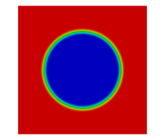
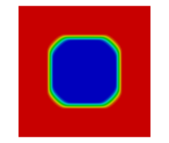
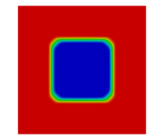
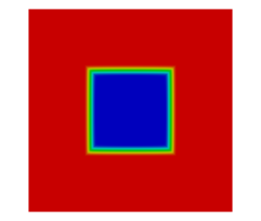
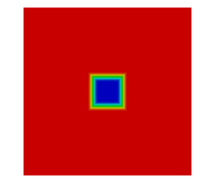
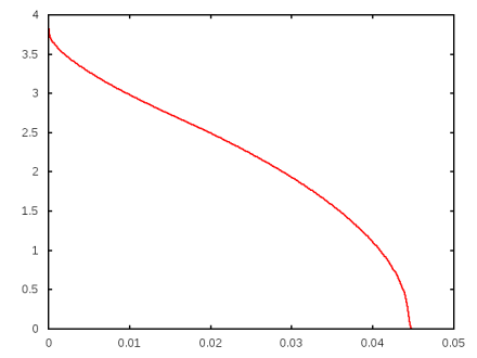
Figure 1: (ani${}_{1}^{(0.01)}$) A phase field approximation for the anisotropic mean curvature flow (12). Snapshots of the solution at times $t=0,\,5\times 10^{-3},\,10^{-2},\,2\times 10^{-2},\,4\times 10^{-2}$. A plot of $\mathcal{E}_{\gamma}^{h}$ below.

A numerical experiment for (18) with the help of the approximation (28a,b), for the Cahn–Hilliard equation (9a–d) can be seen in Figure 2. Here the initial profile is given by two circles with radii $0.2$ and $0.15$. We set $\tau=10^{-6}$ and $T=10^{-4}$. We observe that the two connected components of the inner phase each take on the form of the hexagonal Wulff shape.

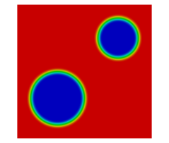
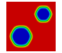
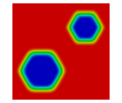
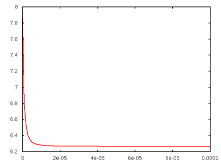
Figure 2: (ani₃) A phase field approximation for anisotropic surface diffusion (18). Snapshots of the solution at times $t=0,\,2\times 10^{-6},\,5\times 10^{-6},\,10^{-5},\,10^{-4}$. A plot of $\mathcal{E}_{\gamma}^{h}$ below.

A repeat of the experiment but now for $b(u)=b_{0}=2$, so that the sharp interface limit is given by the Mullins–Sekerka problem (14a–d), is shown in Figure 3. Here we set $\tau=10^{-5}$ and $T=5\times 10^{-3}$. Now, in contrast to the evolution in Figure 2, the smaller region shrinks so that eventually there is only one connected component of the inner phase. Of course, the final interface is converging to the hexagonal Wulff shape.

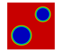
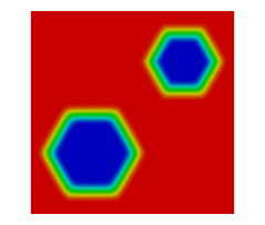
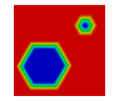
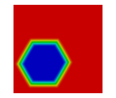
Figure 3: (ani₃) A phase field approximation for the anisotropic Mullins–Sekerka problem (14a–d). Snapshots of the solution at times $t=0,\,10^{-4},\,10^{-3},\,4.6\times 10^{-3},\,5\times 10^{-3}$. A plot of $\mathcal{E}_{\gamma}^{h}$ below.

The remaining computations in this subsection are for the scheme (35a,b). In order to visualize the possible onset of a boundary layer as explained in Remark 3.5, we present a computation for (35a,b) with the initial data $U^{0}=u_{0}=1$. As we set $\alpha=1$, the critical value for $w_{\partial\Omega}$ in (41) is $-\frac{2}{c_{\Psi}}\,\varepsilon^{-1}=-\frac{4}{\pi}\,16\,\pi=-64$. In our numerical computations this lower bound appears to be sharp. In particular, we observe that $U^{n}=1$ is a steady state whenever $w_{\partial\Omega}\geq-64$, but a boundary layer forms already for e.g. $w_{\partial\Omega}=-64-10^{-8}$. As an example, we present a run for $w_{\partial\Omega}=-65$ in Figure 4, where we can clearly see how the boundary layer develops. Once the boundary layer has formed, the inner phase first shrinks and then disappears, leading to the steady state solution $U^{0}=-1$ and $W^{n}=w_{\partial\Omega}$. Note that this phenomenon is completely independent from the choice of anisotropy $\gamma$. The discretization parameters for this experiment were $N_{f}=N_{c}=128$ and $\tau=10^{-5}$ with $T=10^{-3}$.

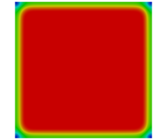
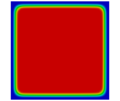
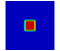
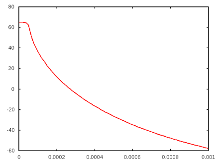
Figure 4: (ani${}_{1}^{(0.01)}$, $w_{\partial\Omega}=-65$) Creation of a boundary layer. Snapshots of the solution at times $t=0,\,4\times 10^{-5},\,5\times 10^{-5},\,\,7\times 10^{-5},\,10^{-3}$. A plot of $\mathcal{F}_{\gamma}^{h}$ below.

Next we simulate the growth of a small crystal, when the sharp interface evolution is given by (14a–c), (15). In particular, we fix $H=8$, $w_{\partial\Omega}=-2$ and $\alpha=0.03$; and we observe that for this choice of parameters the condition (41) is satisfied if we choose $\varepsilon^{-1}=32\,\pi>\frac{50}{3}\,\pi$. A run for (35a,b), when the initial seed has radius $0.1$, with the discretization parameters $N_{f}=4096$, $N_{c}=128$, $\tau=10^{-4}$ and $T=7.5$ is shown in Figure 5. We observe that at first the crystal seed grows, taking on the form of the Wulff shape of $\gamma$. Then the four sides break and become nonconvex, with the four side arms that grow at the corners yielding a shape that is well-known in the numerical simulation of dendritic growth.

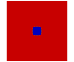
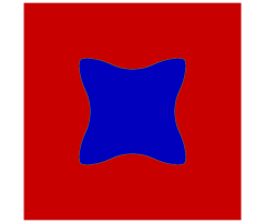
Figure 5: (ani${}_{1}^{(0.3)}$, $w_{\partial\Omega}=-2$, $\varepsilon^{-1}=32\,\pi$, $\Omega=(-8,8)^{2}$) A phase field approximation for the anisotropic Mullins–Sekerka problem (14a–c), (15). Snapshots of the solution at times $t=0,\,1,\,5,\,7,\,7.5$. A plot of $\mathcal{F}_{\gamma}^{h}$ below.

4.2 Numerical results in 3d

A numerical experiment for (12) in 3d with the help of the approximation (32), (28b) for the Allen–Cahn equation (11a–c) can be seen in Figure 6. Here the initial profile is given by a sphere with radius $0.3$. We set $\tau=10^{-4}$ and $T=0.03$. It can be seen that the initially round sphere assumes the cylindrical Wulff shape as it shrinks, before the interface shrinks to a point and disappears completely.

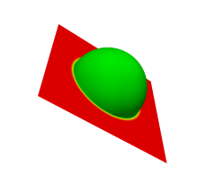
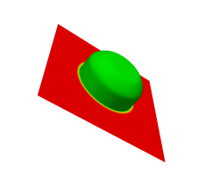
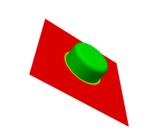
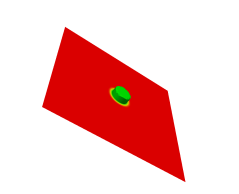
Figure 6: (ani₂) A phase field approximation for the anisotropic mean curvature flow (12). Snapshots of the solution at times $t=0,\,5\times 10^{-3},\,10^{-2},\,1.5\times 10^{-2},\,2\times 10^{-2}$. A plot of $\mathcal{E}_{\gamma}^{h}$ below.

A numerical experiment for (18) with the help of the approximation (28a,b) for the Cahn–Hilliard equation (9a–d) can be seen in Figure 7. Here the initial profile is given by a sphere with radius $0.3$. We set $\tau=10^{-6}$ and $T=10^{-3}$. We can clearly see the evolution from the round sphere to the strongly facetted Wulff shape.

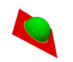
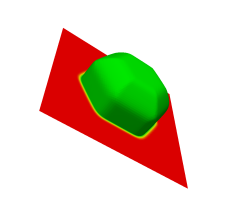
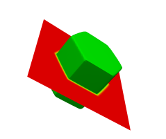
Figure 7: (ani₄) A phase field approximation for anisotropic surface diffusion (18). Snapshots of the solution at times $t=0,\,10^{-5},\,2\times 10^{-5},\,5\times 10^{-5},\,10^{-3}$. A plot of $\mathcal{E}_{\gamma}^{h}$ below.

A numerical approximation for the sharp interface problem (14a–d), is shown in Figure 8. Here the initial interface is given by the boundary of a $8\times 1\times 1$ cuboid with minor side length $0.1$, and we set $\tau=10^{-5}$ and $T=5\times 10^{-3}$. We can observe that during the evolution the elongated facets become bent and nonconvex, before the solution converges to the Wulff shape.

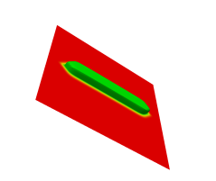
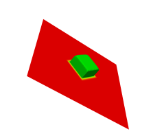
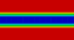
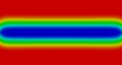
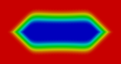
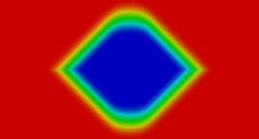
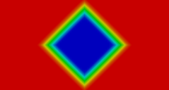
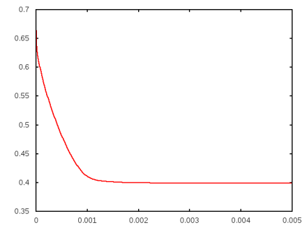
Figure 8: (ani${}_{1}^{\star}$) A phase field approximation for the anisotropic Mullins–Sekerka problem (14a–d). Snapshots of the solution at times $t=0,\,10^{-4},\,5\times 10^{-4},\,10^{-3},\,5\times 10^{-3}$. The middle row shows detailed $2d$ plots of the solution in the $x_{1}$–$x_{2}$ plane. A plot of $\mathcal{E}_{\gamma}^{h}$ below.

References

• [1] H. Abels, H. Garcke, and G. Grün, Thermodynamically consistent, frame indifferent diffuse interface models for incompressible two-phase flows with different densities, Math. Models Methods Appl. Sci., 22 (2012), p. 1150013.
• [2] M. Alfaro, H. Garcke, D. Hilhorst, H. Matano, and R. Schätzle, Motion by anisotropic mean curvature as sharp interface limit of an inhomogeneous and anisotropic Allen-Cahn equation, Proc. Roy. Soc. Edinburgh Sect. A, 140 (2010), pp. 673–706.
• [3] F. Bai, C. M. Elliott, A. Gardiner, A. Spence, and A. M. Stuart, The viscous Cahn–Hilliard equation. I. Computations, Nonlinearity, 8 (1995), pp. 131–160.
• [4] L’. Baňas and R. Nürnberg, Finite element approximation of a three dimensional phase field model for void electromigration, J. Sci. Comp., 37 (2008), pp. 202–232.
• [5] L’. Baňas and R. Nürnberg, A multigrid method for the Cahn–Hilliard equation with obstacle potential, Appl. Math. Comput., 213 (2009), pp. 290–303.
• [6] L’. Baňas and R. Nürnberg, Phase field computations for surface diffusion and void electromigration in ${\mathbb{R}}^{3}$, Comput. Vis. Sci., 12 (2009), pp. 319–327.
• [7] J. W. Barrett, J. F. Blowey, and H. Garcke, Finite element approximation of the Cahn–Hilliard equation with degenerate mobility, SIAM J. Numer. Anal., 37 (1999), pp. 286–318.
• [8] J. W. Barrett, H. Garcke, and R. Nürnberg, Numerical approximation of anisotropic geometric evolution equations in the plane, IMA J. Numer. Anal., 28 (2008), pp. 292–330.
• [9]  , A variational formulation of anisotropic geometric evolution equations in higher dimensions, Numer. Math., 109 (2008), pp. 1–44.
• [10]  , Finite element approximation of coupled surface and grain boundary motion with applications to thermal grooving and sintering, European J. Appl. Math., 21 (2010), pp. 519–556.
• [11]  , On stable parametric finite element methods for the Stefan problem and the Mullins–Sekerka problem with applications to dendritic growth, J. Comput. Phys., 229 (2010), pp. 6270–6299.
• [12]  , Parametric approximation of surface clusters driven by isotropic and anisotropic surface energies, Interfaces Free Bound., 12 (2010), pp. 187–234.
• [13]  , Finite element approximation of one-sided Stefan problems with anisotropic, approximately crystalline, Gibbs–Thomson law, 2012. http://arxiv.org/abs/1201.1802.
• [14]  , Numerical computations of faceted pattern formation in snow crystal growth, Phys. Rev. E, 86 (2012), p. 011604.
• [15]  , Stable phase field approximations of the anisotropic Gibbs–Thomson law with kinetic undercooling, 2012. (in preparation).
• [16] J. W. Barrett, R. Nürnberg, and V. Styles, Finite element approximation of a phase field model for void electromigration, SIAM J. Numer. Anal., 42 (2004), pp. 738–772.
• [17] G. Bellettini and M. Paolini, Anisotropic motion by mean curvature in the context of Finsler geometry, Hokkaido Math. J., 25 (1996), pp. 537–566.
• [18] M. Beneš, Diffuse-interface treatment of the anisotropic mean-curvature flow, Appl. Math., 48 (2003), pp. 437–453. Mathematical and computer modeling in science and engineering.
• [19] M. Beneš, Computational studies of anisotropic diffuse interface model of microstructure formation in solidification, Acta Math. Univ. Comenian. (N.S.), 76 (2007), pp. 39–50.
• [20] L. Blank, M. Butz, and H. Garcke, Solving the Cahn–Hilliard variational inequality with a semi-smooth Newton method, ESAIM Control Optim. Calc. Var., 17 (2011), pp. 931–954.
• [21] J. F. Blowey and C. M. Elliott, The Cahn–Hilliard gradient theory for phase separation with non-smooth free energy. Part II: Numerical analysis, European J. Appl. Math., 3 (1992), pp. 147–179.
• [22] G. Caginalp, An analysis of a phase field model of a free boundary, Arch. Rational Mech. Anal., 92 (1986), pp. 205–245.
• [23] G. Caginalp and X. Chen, Convergence of the phase field model to its sharp interface limits, European J. Appl. Math., 9 (1998), pp. 417–445.
• [24] G. Caginalp and C. Eck, Rapidly converging phase field models via second order asymptotics, Discrete Contin. Dyn. Syst., (2005), pp. 142–152.
• [25] J. W. Cahn, On spinodal decomposition, Acta Metall., 9 (1961), pp. 795–801.
• [26] J. W. Cahn, C. M. Elliott, and A. Novick-Cohen, The Cahn–Hilliard equation with a concentration dependent mobility: motion by minus the Laplacian of the mean curvature, European J. Appl. Math., 7 (1996), pp. 287–301.
• [27] J. W. Cahn and J. E. Hilliard, Free energy of a non-uniform system. I. Interfacial free energy, J. Chem. Phys., 28 (1958), pp. 258–267.
• [28] J. W. Cahn and D. W. Hoffman, A vector thermodynamics for anisotropic surfaces – II. Curved and faceted surfaces, Acta Metall., 22 (1974), pp. 1205–1214.
• [29] S. H. Davis, Theory of Solidification, Cambridge Monographs on Mechanics, Cambridge University Press, Cambridge, 2001.
• [30] J.-M. Debierre, A. Karma, F. Celestini, and R. Guérin, Phase-field approach for faceted solidification, Phys. Rev. E, 68 (2003), p. 041604.
• [31] K. Deckelnick, G. Dziuk, and C. M. Elliott, Computation of geometric partial differential equations and mean curvature flow, Acta Numer., 14 (2005), pp. 139–232.
• [32] C. Eck, Analysis of a two-scale phase field model for liquid-solid phase transitions with equiaxed dendritic microstructure, Multiscale Model. Simul., 3 (2004), pp. 28–49.
• [33]  , Homogenization of a phase field model for binary mixtures, Multiscale Model. Simul., 3 (2004), pp. 1–27.
• [34] C. Eck, H. Garcke, and B. Stinner, Multiscale problems in solidification processes, in Analysis, modeling and simulation of multiscale problems, Springer, Berlin, 2006, pp. 21–64.
• [35] C. M. Elliott, Approximation of curvature dependent interface motion, in The state of the art in numerical analysis (York, 1996), I. S. Duff and G. A. Watson, eds., vol. 63 of Inst. Math. Appl. Conf. Ser. New Ser., Oxford Univ. Press, New York, 1997, pp. 407–440.
• [36] C. M. Elliott and A. R. Gardiner, Double obstacle phase field computations of dendritic growth, 1996. University of Sussex CMAIA Research report 96-19.
• [37] C. M. Elliott and R. Schätzle, The limit of the anisotropic double-obstacle Allen-Cahn equation, Proc. Roy. Soc. Edinburgh Sect. A, 126 (1996), pp. 1217–1234.
• [38] H. Garcke, B. Nestler, and B. Stoth, On anisotropic order parameter models for multi-phase systems and their sharp interface limits, Phys. D, 115 (1998), pp. 87–108.
• [39] H. Garcke, B. Stoth, and B. Nestler, Anisotropy in multi-phase systems: a phase field approach, Interfaces Free Bound., 1 (1999), pp. 175–198.
• [40] C. Gräser and R. Kornhuber, On preconditioned Uzawa-type iterations for a saddle point problem with inequality constraints, in Domain decomposition methods in science and engineering XVI, vol. 55 of Lect. Notes Comput. Sci. Eng., Springer, Berlin, 2007, pp. 91–102.
• [41] C. Gräser, R. Kornhuber, and U. Sack, Time discretizations of anisotropic Allen–Cahn equations, 2011. Matheon Preprint, Berlin.
• [42] C. Gräser, R. Kornhuber, and U. Sack, Nonsmooth Schur–Newton methods for vector-valued Cahn–Hilliard equations, 2012. Matheon Preprint, Berlin.
• [43] M. Hintermüller, M. Hinze, and M. H. Tber, An adaptive finite-element Moreau–Yosida-based solver for a non-smooth Cahn–Hilliard problem, Optim. Methods Softw., 26 (2011), pp. 777–811.
• [44] A. Karma and W.-J. Rappel, Phase-field method for computationally efficient modeling of solidification with arbitrary interface kinetics, Phys. Rev. E, 53 (1996), pp. R3017–R3020.
• [45]  , Quantitative phase-field modeling of dendritic growth in two and three dimensions, Phys. Rev. E, 57 (1998), pp. 4323–4349.
• [46] J. Kim, K. Kang, and J. Lowengrub, Conservative multigrid methods for Cahn–Hilliard fluids, J. Comput. Phys., 193 (2004), pp. 511–543.
• [47] R. Kobayashi, Modeling and numerical simulations of dendritic crystal growth, Phys. D, 63 (1993), pp. 410–423.
• [48] B. Li, J. Lowengrub, A. Rätz, and A. Voigt, Geometric evolution laws for thin crystalline films: modeling and numerics, Commun. Comput. Phys., 6 (2009), pp. 433–482.
• [49] G. B. McFadden, A. A. Wheeler, R. J. Braun, S. R. Coriell, and R. F. Sekerka, Phase-field models for anisotropic interfaces, Phys. Rev. E (3), 48 (1993), pp. 2016–2024.
• [50] M. Paolini, Fattening in two dimensions obtained with a nonsymmetric anisotropy: numerical simulations, in Proceedings of the Algoritmy’97 Conference on Scientific Computing (Zuberec), vol. 67, 1998, pp. 43–55.
• [51] A. Schmidt and K. G. Siebert, Design of Adaptive Finite Element Software: The Finite Element Toolbox ALBERTA, vol. 42 of Lecture Notes in Computational Science and Engineering, Springer-Verlag, Berlin, 2005.
• [52] J. E. Taylor and J. W. Cahn, Linking anisotropic sharp and diffuse surface motion laws via gradient flows, J. Statist. Phys., 77 (1994), pp. 183–197.
• [53] J. E. Taylor, J. W. Cahn, and C. A. Handwerker, Geometric models of crystal growth, Acta Metall. Mater., 40 (1992), pp. 1443–1474.
• [54] A. A. Wheeler and G. B. McFadden, A $\xi$-vector formulation of anisotropic phase-field models: $3$D asymptotics, European J. Appl. Math., 7 (1996), pp. 367–381.
• [55] S. Wise, J. Kim, and J. Lowengrub, Solving the regularized, strongly anisotropic Cahn–Hilliard equation by an adaptive nonlinear multigrid method, J. Comput. Phys., 226 (2007), pp. 414–446.