Gaussian Equilibration

Abstract

A finite quantum system evolving unitarily equilibrates in a probabilistic fashion. In the general many-body setting the time-fluctuations of an observable $\mathcal{A}$ are typically exponentially small in the system size. We consider here quasi-free Fermi systems where the Hamiltonian and observables are quadratic in the Fermi operators. We first prove a novel bound on the temporal fluctuations $\Delta\mathcal{A}^{2}$ and then map the equilibration dynamics to a generalized classical XY model in the infinite temperature limit. Using this insight we conjecture that, in most cases, a central limit theorem can be formulated leading to what we call Gaussian equilibration: observables display a Gaussian distribution with relative error $\Delta\mathcal{A}/\overline{\mathcal{A}}=O(L^{-1/2})$ where $L$ is the dimension of the single particle space. The conjecture, corroborated by numerical evidence, is proven analytically under mild assumptions for the magnetization in the quantum XY model and for a class of observables in a tight-binding model. We also show that the variance is discontinuous at the transition between a quasi-free model and a non-integrable one.

I Introduction

Out of equilibrium and equilibration dynamics of closed quantum systems have been recently at the center of a renewed and intense interest (Kinoshita et al., 2006; Calabrese and Cardy, 2006; Hofferberth et al., 2007; Rigol et al., 2008; Linden et al., 2009; Campos Venuti and Zanardi, 2010a; Campos Venuti et al., 2011). In particular the issue whether quantum integrability plays a key role in equilibration and, if so, which one, has been investigated by several authors (Rigol et al., 2007; Kollath et al., 2007; Barthel and Schollwöck, 2008). In this paper we will address this problem along the lines of the probabilistic approach to quantum equilibration advocated in (Campos Venuti and Zanardi, 2010a, b; Campos Venuti et al., 2011). Here the central object is the (infinite time) full time statistics of the expectation value of a quantum observable. We will focus on a particular, yet very important class of quantum integrable systems: quasi-free fermionic systems, i.e. systems where both the Hamiltonian and the observable are quadratic in the canonical Fermi operators. Using fairly general central-limit type arguments as well as explicit analytic examples we will argue that a sharp distinctive feature of these systems, as opposed to the general interacting ones, is an exponential enhancement of the amplitude of the temporal fluctuations of a quadratic observable around its mean value. This appears to be a precise and quantitative way to make sense of the common folklore that integrability leads to a poorer (or no) equilibration.

The system is initialized in a generic state $\rho_{0}$ with $N$ particles and both the evolution Hamiltonian $H$ and the observable $A$ are quadratic in the fermionic operators . The Hamiltonian is $H=\sum_{x,y}c_{x}^{\dagger}M_{x,y}c_{y}=c^{\dagger}Mc$ (notation $c^{\dagger}=\left(c_{1}^{\dagger},\ldots,c_{L}^{\dagger}\right)$, $L$ number of sites). The general quadratic observable has the form $A=\sum_{x,y}c_{x}^{\dagger}a_{x,y}c_{y}=c^{\dagger}ac$. We will assume that $\left\|a\right\|_{\infty}=O\left(1\right)$ as this guarantees that the expectation values of $A$ scales at most extensively with the system size . The main object of investigation is $\mathcal{A}\left(t\right)=\mathrm{tr}\left(Ae^{-itH}\rho_{0}e^{itH}\right)$. Exploiting the quadratic nature of the problem and introducing the covariance matrix $R_{y,x}:=\mathrm{tr}\left(\rho_{0}c_{x}^{\dagger}c_{y}\right)$ ($0\leq R\leq\leavevmode{\rm 1\mkern-4.8muI}$) one can show that the expectation value $\mathcal{A}\left(t\right)$ reduces to a trace in the one-particle space:

$$\mathcal{A}\left(t\right)=\mathrm{tr}\left(ae^{-itM}Re^{itM}\right)\,.$$ (1)

Eq. (1) is perfectly analogous to its many-body version $\mathcal{A}\left(t\right)=\mathrm{tr}\left(Ae^{-itH}\rho_{0}e^{itH}\right)$ with $R$ playing the role of the initial state $\rho_{0}$. There is however one importance difference: while $\mathrm{tr}\rho_{0}=1$ one has $\mathrm{tr}R=N=\nu L$ , i.e. is extensive (we defined $\nu=N/L$ the filling factor).

For unitary evolution in finite systems, the density matrix $\rho\left(t\right)=e^{-itH}\rho_{0}e^{itH}$ does not converge neither in the strong nor in the weak topology (Campos Venuti and Zanardi, 2010a). Equilibration must be formulated in probabilistic terms. Given the observation time window $\left[0,T\right]$, the observable $\mathcal{A}\left(t\right)$ has probability $P_{A}\left(\alpha\right)d\alpha$ of being in the interval $\left[\alpha,\alpha+d\alpha\right]$, where the probability density is given by $P_{A}\left(\alpha\right)=\overline{\delta\left(\mathcal{A}\left(t\right)-\alpha\right)^{T}}$, and the time average operation is $\overline{f^{T}}=T^{-1}\int_{0}^{T}f\left(t\right)dt$. For simplicity we will always take the limit $T\to\infty$ when taking time average and write simply $\overline{f}$ in place of $\overline{f^{\infty}}$. Roughly speaking an observable $A$ equilibrates if its probability density $P_{A}\left(\alpha\right)$ is highly peaked around its mean $\overline{\mathcal{A}\left(t\right)}=\mathrm{tr}\left(A\overline{\rho}\right)$ (Campos Venuti and Zanardi, 2010a). The role of equilibrium state is played by the time-averaged density matrix $\overline{\rho}.$

The question we are going to address here is: what is the size of the fluctuations of $P_{A}\left(\alpha\right)$ for observables $A$ in this quasi-free setting?

Before tackling this question and concentrate on fluctuations, let us point out a few remarks on the nature of the equilibrium state itself. If the spectrum is non-degenerate, the average, dephased, state $\overline{\rho}$ has the form $\overline{\rho}=\sum_{n}p_{n}|n\rangle\langle n|$ where $|n\rangle$ are many-body eigenstate of $H$ corresponding to energy $E_{n}$ and $p_{n}=\langle n|\rho_{0}|n\rangle$. The powers of the Hamiltonian $H^{n}$, $n=0,1,\ldots,d-1$ are linearly independent if there are $d$ different eigenvalues $E_{n}$ and if the spectrum is non-degenerate $d$ coincides with the Hilbert space dimension . In this latter case the average state can always be written in the form $\overline{\rho}=\exp\left[\sum_{k=0}^{d-1}\alpha_{k}H^{k}\right]$, the so called GGE (generalized Gibbs ensemble) (Rigol et al., 2007). The coefficients $\alpha_{n}$ depend on the initial state $\rho_{0}$ and on the eigenvectors $\{|n\rangle\}$. The condition to write the coefficients $\alpha_{n}$ in terms of the $p_{n}$ is precisely that of the invertibility of the Vandermonde matrix $V_{n,k}=\left(E_{n}\right)^{k-1}$ ($n,k=1,\ldots,d$), i.e., once again, non-degeneracy of the spectrum, since $\det V=\prod_{n<k}\left(E_{k}-E_{n}\right)$. The relation expressing the $p_{n}$’s in terms of the $\alpha_{k}$’s is: $p_{n}=\exp\left[\sum_{k=0}^{d-1}\alpha_{k}E_{n}^{k}\right]$. Since $\overline{\rho}=\exp\sum_{n}\ln p_{n}|n\rangle\langle n|=\exp\sum_{k=0}^{d-1}\sum_{n}\alpha_{k}E_{n}^{k}|n\rangle\langle n|$ , the inverse relation is, in vector notation $\boldsymbol{\alpha}=V^{-1}\ln\boldsymbol{p}$. The inverse of the Vandermonde matrix can be found explicitly by expanding the identity $|n\rangle\langle n|=\prod_{k\neq n}\frac{H-E_{k}}{E_{n}-E_{k}}$, multiplying by $\ln p_{n}$, summing over $n$ and exponentiating see

Let us now go back to the context of Eq. (1). Since $0\leq R\left(t\right)\leq\leavevmode{\rm 1\mkern-4.8muI}$ the time averaged covariance $\overline{R}=\overline{e^{-itM}Re^{itM}}$ satisfies $0\leq\overline{R}\leq\leavevmode{\rm 1\mkern-4.8muI}$ and so defines a Gaussian state $\rho_{\overline{R}}$ with covariance $\overline{R}$. Moreover, since $\mathrm{tr}R\left(t\right)=N$, for all $t$, $\mathrm{tr}\overline{R}=N$, $\rho_{\overline{R}}$ is a Gaussian state with $N$ particles. Now, for what concerns quadratic observables of the kind $A=c^{\dagger}ac$, their time average expectation value is the same as that obtained with $\rho_{\overline{R}}$: $\overline{\mathcal{A}}=\mathrm{tr}a\overline{R}=\mathrm{tr}A\rho_{\overline{R}}$. In other words the states $\overline{\rho}$ and $\rho_{\overline{R}}$ are the same when restricted to quadratic observables. A generic Gaussian state can be written in the form $\rho_{R}={\cal N}\exp\left(c^{\dagger}G(R)c\right)$ where $G(R):=\log[R(1-R)^{-1}]$ (Peschel, 2003) and ${\cal N}$ is a normalization constant. From this it immediately follows that $\rho_{\overline{R}}$ can be written as $\rho_{\overline{R}}={\cal N}\exp\sum_{k}\lambda_{k}c_{k}^{\dagger}c_{k}$ where $c_{k}$’s are eigenmodes of $H$ and coincides with equation (8) of (Rigol et al., 2007). When the system equilibrates i.e., ${\cal A}(t)\to\mathrm{tr}\left(A\rho_{\overline{R}}\right)$ this remark shows the validity of the GGE for any initial state $\rho_{0}$ and all quadratic observables. Indications that $\overline{\rho}$ converges to $\rho_{\overline{R}}$ in some sense as the size increases were indeed already present in the literature. For instance in (Lanford and Robinson, 1972) it was shown that, in the thermodynamic limit, $\rho\left(t\right)\to\rho_{\overline{R}}$ weakly as $t\to\infty$, while in (Cramer et al., 2008; Cramer and Eisert, 2010) a particular form of strong convergence was derived, when considering subsystems (though for a Bosonic system).

II A bound on the variance

Assuming the non-resonant condition on the energies ($E_{n}-E_{m}=E_{p}-E_{q}$ implies $n=m$ and $p=q$ or $n=p$ and $m=q$), Reimann has shown (Reimann, 2008) that the temporal fluctuations $\Delta\mathcal{A}^{2}=\overline{\left(\mathcal{A}\left(t\right)-\overline{\mathcal{A}}\right)^{2}}$ satisfy $\Delta\mathcal{A}^{2}\leq\mathrm{diam}\left(A\right)^{2}\mathrm{tr}\overline{\rho}^{2}$ where $\mathrm{diam}\left(A\right)$ is the maximum minus the minimum eigenvalue of $A$. Now in general, for most initial states $\rho_{0}$, the purity $\mathrm{tr}\overline{\rho}^{2}$ is exponentially small in the system size implying exponentially small fluctuations. Here is one argument. First note that $\mathrm{tr}\overline{\rho}^{2}=\overline{\mathcal{L}\left(t\right)}$ with $\mathcal{L}\left(t\right)$ being the Loschmidt echo: $\mathcal{L}\left(t\right)=\left|\langle\psi_{0}|e^{-itH}|\psi_{0}\rangle\right|^{2}$ which admits the following cumulant expansion $\mathcal{L}\left(t\right)=\exp\left[2\sum_{n=1}^{\infty}\left(-t^{2}\right)^{n}\langle H^{2n}\rangle_{c}/\left(2n\right)!\right]$ (Campos Venuti and Zanardi, 2010a). Here $\langle H^{2n}\rangle_{c}$ are the cumulants of $H$ computed with $\rho_{0}$. The point is that if $\rho_{0}$ is sufficiently clustering, but not an eigenstate of $H$, all the cumulants are extensive in the system size and non-zero. Then $\mathcal{L}\left(t\right)=\exp\left[-L^{D}g\left(t\right)+\mathrm{corrections}\right]$ where $g\left(t\right)\geq 0$ does not depend on the size and, for sufficiently large $L$ one has $\overline{\mathcal{L}}\leq\exp\left[-L^{D}\min_{t}g\left(t\right)\right]$ .

In the quasi-free setting the non-resonant condition does not hold. Let us then seek for the analogous of the bound of Reimann in our quasi-free case. Let the one-particle Hamiltonian have the following diagonal form $M=\sum_{k}\Lambda_{k}|k\rangle\langle k|$. The time averaged covariance matrix is then $\overline{R}=\sum_{k}\langle k|R|k\rangle|k\rangle\langle k|$. We also define $F_{k,q}=\langle k|a|q\rangle\langle q|R|k\rangle$. Assuming the non-resonance condition for the one-particle spectrum, one gets $\Delta\mathcal{A}^{2}=\mathrm{tr}F^{2}-\sum_{k}\left(F_{k,k}\right)^{2}\leq\mathrm{tr}F^{2}=\sum_{k,q}\left|\langle k|a|q\rangle\right|^{2}\left|\langle q|R|k\rangle\right|^{2}$. Now $R$ is a non-negative operator and so induces a (possibly degenerate) scalar product which satisfies Cauchy-Schwarz inequality: $\left|\langle q|R|k\rangle\right|^{2}=\left|\langle q|k\rangle_{R}\right|^{2}\leq\langle q|q\rangle_{R}\langle k|k\rangle_{R}=\langle q|R|q\rangle\langle k|R|k\rangle$. This leads us to

$$\Delta\mathcal{A}^{2}\leq\mathrm{tr}\left(a\overline{R}a\overline{R}\right)\leq\left\|a\right\|_{\infty}^{2}\mathrm{tr}\overline{R}^{2}$$ (2)

Now, since $0\leq\overline{R}\leq\leavevmode{\rm 1\mkern-4.8muI}$, $\mathrm{tr}\overline{R}^{2}\leq\mathrm{tr}\overline{R}=\mathrm{tr}R=N$, we finally obtain $\Delta\mathcal{A}^{2}\leq\left\|a\right\|_{\infty}^{2}\nu L\,.$ While equation (2) is the quasi-free analog of the Reimann’s bound it implies some important differences with respect to the general (non-free) case. Consider the situation where the observable $A$ is extensive. In the non-free case the diameter of $A$ is extensive, i.e. $\mathrm{diam}\left(A\right)=O\left(L^{D}\right)$ in $D$ spatial dimensions. Moreover, the minimum value of the purity $\mathrm{tr}\overline{\rho}^{2}$ is $1/d$ and so is exponentially small in the system size. In the quasi-free setting, instead, the minimum value of $\mathrm{tr}\overline{R}^{2}$ in Eq. (2) is $\min\mathrm{tr}\overline{R}^{2}=N^{2}/L=\nu^{2}L$, since $\overline{R}/N$ defines a density matrix for which the minimum purity is the inverse of the matrix dimension $L$. All in all, recalling that $\left\|a\right\|_{\infty}=O\left(1\right),$ for extensive observables, the minimum of the bound to the variance is $O\left(L^{2}e^{-\gamma L}\right)$, $\gamma>0$, (for systems of linear size $L$), whereas in the quasi-free setting one has $O\left(L\right)$. This seems to hint at the fact that fluctuations in the quasi-free setting are proportional to the system size and are hence much larger than in the non-free case where they are exponentially small in the volume. Of course Eq. (2) is just an upper bound, and nothing prevents, in principle, from having a much smaller variance. For example, whenever the initial state or the observable commute with the Hamiltonian, $\mathcal{A}\left(t\right)$ is constant and its fluctuations are zero. We will always avoid such pathological situations. In the following, instead, we will argue that the extensive behavior of the fluctuations, in quasi-free systems, is in fact quite general, leading to a $1/\sqrt{L}$ scaling of the relative error $\sqrt{\Delta\mathcal{A}^{2}}/\overline{\mathcal{A}}$ for a generic observable. Indeed such a $1/\sqrt{L}$ scaling has been observed to hold for a quadratic Hamiltonian even for more general observables (see supplementary material of (Cassidy et al., 2011)) and even in presence of disorder except for quenches into a localized phase (Gramsch and Rigol, 2012).

III Mapping to a classical XY model

Let us write again the generic expectation value (1) in the basis which diagonalizes $M$: $\mathcal{A}\left(t\right)=\overline{\mathcal{A}}+2\sum_{k<q}\left|F_{k,q}\right|\cos\left(t\left(\Lambda_{k}-\Lambda_{q}\right)+\phi_{k,q}\right)$ with $\phi_{k,q}=\arg F_{k,q}$. To obtain information on the probability density $P_{A}\left(\alpha\right)$ we consider the generating function $\chi_{A}\left(\lambda\right):=\overline{e^{\lambda\left(\mathcal{A}\left(t\right)-\overline{\mathcal{A}}\right)}}$. Now we observe that if the (one-particle) energies are rationally independent (RI), as a consequence of a theorem on the averages, the infinite time average of $\mathcal{A}\left(t\right)$ is the same as the uniform average over the torus $\mathbb{T}^{L}$. In this case the generating function $\chi_{A}\left(\lambda\right)$ is exactly given by the partition function of the generalized, classical XY model with energy $E\left(\boldsymbol{\theta}\right)=2\sum_{k<q}\left|F_{k,q}\right|\cos\left(\theta_{k}-\theta_{q}+\phi_{k,q}\right)$ and inverse temperature $\beta=-\lambda$. The matrix $\left|F_{k,q}\right|$ defines the lattice of the interactions while the phases $\phi_{k,q}$ give the offset from which the angles are measured. Note that the behavior of the density $P_{A}\left(\alpha\right)$ is dictated by $\chi_{A}\left(\lambda\right)$ in a neighborhood of $\lambda=0$ which corresponds to infinite temperature of the classical XY model.

It is not difficult to engineer a situation which exactly reproduces the standard XY model in $D$-dimension. For example, it suffices to consider the Hamiltonian $H=\sum_{\boldsymbol{x}}\mu_{\boldsymbol{x}}c_{\boldsymbol{x}}^{\dagger}c_{\boldsymbol{x}}$, with $\mu_{\boldsymbol{x}}$ RI ($\boldsymbol{x}$ is a point of a $D$-dimensional lattice), choose the observable $A=\sum_{\langle\boldsymbol{x},\boldsymbol{y}\rangle}c_{\boldsymbol{x}}^{\dagger}c_{\boldsymbol{y}}$ ($\langle\boldsymbol{x},\boldsymbol{y}\rangle$ indicates nearest neighbor) and initial state $|\psi_{0}\rangle=L^{-1/2}\sum_{\boldsymbol{x}}|\boldsymbol{x}\rangle=c_{\boldsymbol{k}=0}^{\dagger}|0\rangle$. In this case the partition function $\mathcal{Z}$ (free-energy $\mathcal{F}$) of the classical $D$-dimensional XY model is precisely the characteristic function of the observable $A$: $\mathcal{Z}=\chi_{A}\left(\lambda\right)$ ($\mathcal{F}=\ln\chi_{A}\left(\lambda\right)$). In fact in this case $a_{\boldsymbol{x},\boldsymbol{y}}=\delta_{\langle\boldsymbol{x},\boldsymbol{y}\rangle}$ while $R_{\boldsymbol{x},\boldsymbol{y}}=1/L$ so that $F_{\boldsymbol{x},\boldsymbol{y}}=L^{-1}\delta_{\langle\boldsymbol{x},\boldsymbol{y}\rangle}$ which defines the nearest neighbor hyper-cubic graph.

We would like to stress here that the one-particle space has a natural underlying geometric structure. For instance, the labels $k,q$ represent points in momentum (real) space in a superfluid (localized) phase and the distance $\left|k-q\right|$ is well defined. Now, when the matrix elements $\left|F_{k,q}\right|$ decay sufficiently fast as $\left|k-q\right|\to\infty$ the corresponding XY model is well defined in the thermodynamic limit, i.e. the intensive free energy has a limit as $L\to\infty$. This happens for instance in case $\left|F_{k,q}\right|$ decays exponentially in $\left|k-q\right|$ or if one has $\left|F_{k,q}\right|\sim 1/\left|k-q\right|^{\gamma}$ with $\gamma>D$. When this is the case one has $\chi_{A}\left(\lambda\right)=\exp L^{D}f\left(\lambda\right)$ where $f\left(\lambda\right)$ is the free energy per site. Moreover, under these conditions, one expects $f\left(\lambda\right)$ to be analytic in the high temperature, $\lambda=0$, limit, implying that all the cumulants of $\mathcal{A}\left(t\right)$ are extensive. From this we immediately draw the central limit theorem (CLT): as $L\to\infty$ the variable $(\mathcal{A}\left(t\right)-\overline{\mathcal{A}})/L^{D/2}$ tends in distribution to a Gaussian with zero mean and finite variance given by $\partial_{\lambda=0}^{2}f\left(\lambda\right)$. We call this situation Gaussian equilibration. It is important to stress that one cannot have Gaussian equilibration in the non-free setting otherwise all the cumulants would scale in the same way. Instead in the non-free setting one expects extensive average but variance exponentially small in the volume.

We will now further corroborate these arguments with two examples where indeed Gaussian equilibration can be proven or shown.

IV Quench on the quantum XY model

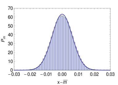
Figure 1: Full distribution for the transverse magnetization per site $m\left(t\right)=\langle\sigma_{i}^{z}\left(t\right)\rangle$ around its mean for $L=40$. The quench is performed from ($\gamma_{0}=\gamma_{1}=1$) $\left(h_{0}=2\right)\to\left(h_{1}=4\right)$. The histogram is obtained sampling $m\left(t\right)$ at 200,000 random times uniformly distributed in $[0,T_{\mathrm{max}}]$ with $T_{\mathrm{max}}=100,000$. The thick curve is a Gaussian with zero mean and variance $\sigma^{2}=L^{-2}\sum_{k>0}W_{k}^{2}/2$ as computed in (Campos Venuti and Zanardi, 2010a).

The Hamiltonian is given in terms of Pauli spin operators $\sigma_{i}^{x,y,x}$ (we use periodic boundary conditions)

$$H=-\sum_{i=1}^{L}\left[\left(\frac{1+\gamma}{2}\right)\sigma_{i}^{x}\sigma_{i+1}^{x}+\left(\frac{1-\gamma}{2}\right)\sigma_{i}^{y}\sigma_{i+1}^{y}+h\sigma_{i}^{z}\right]$$ (3)

In the quench scenario, the initial state is the ground state $|\psi_{0}\rangle$ of the Hamiltonian with parameters $(\gamma_{0},h_{0})$. The parameters are then suddenly changed and $|\psi_{0}\rangle$ is evolved with the Hamiltonian corresponding to $(\gamma_{1},h_{1})$.

The model in Eq. (3) has been long used as a testbed for the study of quantum phase transitions in many body systems, and more recently in the realm of out-of equilibrium unitary dynamics. See (Lieb et al., 1961; Barouch et al., 1970) and the more recent monumental (Calabrese et al., 2012) for more details and references. A Jordan-Wigner transformation brings Eq. (3) to a quadratic form in Fermi operators. Since $\sigma_{i}^{z}$ in terms of Fermi operators is $\sigma_{i}^{z}=2c_{i}^{\dagger}c_{i}-1$, the transverse, total magnetization $M(t)=\sum_{i}\langle\sigma_{i}^{z}\left(t\right)\rangle$ is a quadratic observable. Its expectation value in the quench setting is given by (Barouch et al., 1970; Campos Venuti and Zanardi, 2010a): $M\left(t\right)=2\sum_{k>0}\cos\vartheta_{k}^{\left(1\right)}\cos\left(\delta\vartheta_{k}\right)+\sin\vartheta_{k}^{\left(1\right)}\sin\left(\delta\vartheta_{k}\right)\cos\left(t\Lambda_{k}^{\left(1\right)}\right)$ where $\tan\vartheta_{k}^{\left(i\right)}=-\gamma_{i}\sin k/\left(h_{i}+\cos k\right)$, $\delta\vartheta_{k}=\vartheta_{k}^{\left(1\right)}-\vartheta_{k}^{\left(0\right)}$ and $\Lambda_{k}^{\left(i\right)}=2\sqrt{\left(\gamma_{i}\sin k\right)^{2}+\left(h_{i}+\cos k\right)^{2}}$ are the one-particle energies. The quasi-momenta are quantized according to $k=\pi\left(2n+1\right)/L$, $n=0,1,\ldots,L/2-1$. At this point it seems quite natural to expect that the energies $\Lambda_{k}^{\left(1\right)}$ are rationally independent. Indeed one can show that the numbers $\cos(k_{n})$ $k_{n}=\pi\left(2n+1\right)/L$, $n=1,2,\ldots,(L-1)/2$ are rationally independent for $L$ prime (Campos Venuti et al., 2011). Given the form of the dispersion we may expect that the requirement that $L$ is prime may be removed.

Assuming rational independence of the one-particle energies $\Lambda_{k}^{\left(1\right)}$, the corresponding classical XY model has energy $E\left(\boldsymbol{\theta}\right)=\sum_{k>0}W_{k}\cos(\theta_{k})$ with $W_{k}=\sin\vartheta_{k}^{\left(1\right)}\sin\left(\delta\vartheta_{k}\right)$. Each classical spin ’$k$’ interacts with an external field along a fixed axis with strength $W_{k}$. The partition function factorizes, each integral over $\theta_{k}$ gives a Bessel function $I_{0}\left(\lambda W_{k}\right)$ and we obtain $\overline{e^{\lambda\left(M(t)-\overline{M}\right)}}=\exp\sum_{k>0}\ln\left(I_{0}\left(\lambda W_{k}\right)\right)$. Clearly $M\left(t\right)-\overline{M}$ is a sum of independent random variables, each with zero mean and variance $W_{k}^{2}/2$.

Now, under the –quite reasonable– assumption of rational independence of the one-particle energies, one can prove Gaussian equilibration for the observable $M\left(t\right)$. More precisely one can show that for any value of parameters $(\gamma_{0},h_{0})\neq(\gamma_{1},h_{1})$, the variable $(M-\overline{M})/\sqrt{L}$ as $L\to\infty$ tends in distribution to a Gaussian with zero mean and variance $\left(2\pi\right)^{-1}\int_{0}^{\pi}(W_{k}^{2}/2)\,dk$.

We can prove this result by showing that the Lyapunov condition is satisfied so that the central limit theorem follows from Lindeberg’s theorem (see e.g. (Billingsley, 2012)). Following the notation of (Billingsley, 2012) we have $s_{L}^{2}=\sum_{k}\sigma_{k}^{2}=\sum_{k>0}W_{k}^{2}/2\to L\left(4\pi\right)^{-1}\int_{0}^{\pi}W_{k}^{2}\,dk$. Then, with $\delta=1$ $\overline{\left|X_{k}\right|^{2+\delta}}=4/(3\pi)\left|W_{k}\right|^{3}$. The Lyapunov’s condition with $\delta=1$ amounts to the vanishing of the following quantity as $L\to\infty$:

$$\frac{1}{s_{L}^{3}}\sum_{k>0}\overline{\left|X_{k}\right|^{3}}\stackrel{{\scriptstyle L\to\infty}}{{\longrightarrow}}\frac{1}{\sqrt{L}}\frac{16}{3\sqrt{\pi}}\frac{\int_{0}^{\pi}\left|W_{k}\right|^{3}dk}{\left(\int_{0}^{\pi}\left|W_{k}\right|^{2}dk\right)^{3/2}}\,.$$ (4)

Indeed the RHS of Eq. (4) goes to zero as $L\to\infty$ since $\left|W_{k}\right|\leq 2$ for all $k$ and $\left|W_{k}\right|\neq 0$ for almost any $k$ for $(\gamma_{0},h_{0})\neq(\gamma_{1},h_{1})$.

Remark

For small quench close to a critical point, the function $W_{k}\simeq\sin(\vartheta_{k}^{\left(1\right)})(\partial\vartheta_{k}/\partial x)\,dx$ ($x$ is the quenched variable, $x=\lambda,h$), becomes highly peaked (for instance, the peak is around $k=\pi$ close to the Ising critical point at $h=1$ and $W_{k}/dx$ diverges as $1/k$). For finite $L$ and sufficiently small quench, few terms $W_{k}$ dominate and one can obtain (for finite $L$) a non-Gaussian distribution. Indeed, as discussed in detail in (Campos Venuti and Zanardi, 2010b), this is the case in general: for small quenches close to a quantum critical point, observables become a sum of few independent random variables and the distribution acquires a universal double-peaked form.

In figure 1 we show a plot of the distribution of the transverse magnetization per site $m\left(t\right)=M\left(t\right)/L$ for the equilibration dynamics undergoing a quantum quench. The distribution agrees very well with a Gaussian with variance $\sigma^{2}=L^{-2}\sum_{k>0}W_{k}^{2}/2$ obtained considering $m\left(t\right)$ as a sum of independent variables (Campos Venuti and Zanardi, 2010a). This in turns shows that the assumptions of rational independence seems to be justified or at least that the number of relations among the frequencies is sufficiently small as not to break the CLT. Note that $L$ is not a prime in fig. 1. By only checking that the one particle spectrum is non-degenerate, it is easy to prove that the variance is $\Delta m^{2}=L^{-2}\sum_{k>0}W_{k}^{2}/2$ (Campos Venuti and Zanardi, 2010a). Since $W_{k}$ is a bounded function this implies immediately that $\Delta m^{2}=O\left(L^{-1}\right)$, in accordance with the Gaussian equilibration prediction.

V Tight binding model

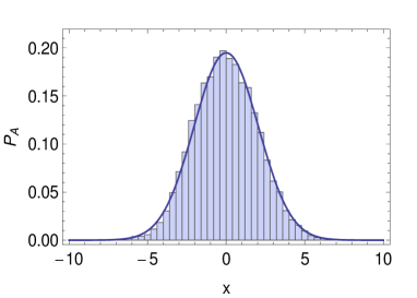
Figure 2: Full distribution for the observable $A=\sum_{x=1}^{\ell}c_{x}^{\dagger}c_{x}$ around its mean for $L=201$, $N=100$, $\ell=101$. The histogram is obtained sampling $\mathcal{A}\left(t\right)$ at 240,000 random times uniformly distributed in $[0,T_{\mathrm{max}}]$ with $T_{\mathrm{max}}=180,000$. The thick curve is a Gaussian with zero mean and variance $\sigma^{2}=0.0208L$ as computed in the text.

We consider here the 1-$D$ tight binding model $H=\sum_{x}\left(c_{x}^{\dagger}c_{x+1}+\mathrm{h.c.}\right)$ with twisted boundary conditions $c_{L+1}=c_{1}e^{i\theta L}$ as proposed in (Tasaki, 2010). As quadratic observable we take $A$ with diagonal one-particle matrix: $A=\sum_{x=1}^{\ell}c_{x}^{\dagger}c_{x}$. The system is initialized setting all the $N$ particles say to the left of the chain, i.e. the initial covariance matrix is $R=\mathrm{diag}\left(1,1,\ldots,1,0,\ldots,0\right)$ with $N$ ones and $L-N$ zeros on the diagonal. The observable $A$ is extensive for $\ell=\alpha L$, and the thermodynamic limit is given by $\alpha=\ell/L$, $\nu=N/L$ constant and $L\to\infty$. The time evolved observable reads $\mathcal{A}\left(t\right)=\sum_{k,q}g_{N}\left(k-q\right)g_{\ell}\left(q-k\right)e^{-it\left(\Lambda_{k}-\Lambda_{q}\right)}$ where the function $g_{\ell}\left(\xi\right)$ is given by $g_{\ell}\left(\xi\right)=L^{-1}\sum_{x=1}^{\ell}e^{-ix\xi}$. The matrix $F_{k,q}$ depends only on the difference $k-q$: $F_{k,q}=f\left(k-q\right)=g_{N}\left(k-q\right)g_{\ell}\left(q-k\right)$. The eigen-energies are given by $\Lambda_{k}=2\cos\left(k+\theta\right)$ and the quasimomenta can be considered quantized as $k=2\pi n/L$, $n=0,1,\ldots,L-1$. For $\theta=0$ the energies are degenerate as $\Lambda_{k}=\Lambda_{\pi-k}$ but for most of the $\theta$, $\pi-k$ does not belong to the Brillouin zone and the energies are non-degenerate. In this case the average is $\overline{\mathcal{A}}=\sum_{k}g_{N}\left(0\right)g_{\ell}\left(0\right)=L\nu\alpha$. Still the $\Lambda_{k}$ cannot be RI as $0=\mathrm{tr}M=\sum_{k}\Lambda_{k}$, however it is likely that there are few relations among the energies. In fact Tasaki showed (Tasaki, 2010) that for $L$ odd and for most of the $\theta\in(0,\pi/L)$, the one-particle energies satisfy the non-resonant condition. This implies that, for most $\theta$, the variance is given by

$$\Delta\mathcal{A}^{2}=\sum_{k,q}\left|g_{N}\left(k-q\right)g_{\ell}\left(q-k\right)\right|^{2}-\sum_{k}\left[g_{N}\left(0\right)g_{\ell}\left(0\right)\right]^{2}.$$

The double sum above can be evaluated going back to real space with result $L^{-2}\left[N\ell^{2}-\ell\left(\ell^{2}-1\right)/3\right]$ (assuming $N\geq\ell$ otherwise swap $N$ with $\ell$). This proves analytically that, besides the average, also the second cumulant –the variance– is extensive and in particular one has $\Delta\mathcal{A}^{2}=L\left(\nu\alpha^{2}-\frac{\alpha^{3}}{3}-\nu^{2}\alpha^{2}\right)+O\left(L^{-1}\right)$.

On the other hand, using methods borrowed from statistical mechanics, we can get an approximate analytic expression for the whole cumulant generating function. In this approximation all the cumulants will turn out to be extensive implying Gaussian equilibration for $\mathcal{A}\left(t\right)$ (see figure 2). We first assume rational independence of the energies $\Lambda_{k}$ so that the problem is mapped to an classical XY model. A single (or a few) relation among the energies is a sort of boundary condition for the classical model and is not expected to change the leading, bulk, term. The energy of the classical model for the translation invariant case is $E\left(\boldsymbol{\theta}\right)=2\sum_{d=1}^{(L-1)/2}\left|f\left(d\right)\right|\sum_{x=1}^{L}\cos\left(\left(\tilde{\theta}_{x+d}-\tilde{\theta}_{x}\right)+\phi_{d}\right)$ ($\phi_{d}=\arg f\left(d\right)$ and $\tilde{\theta}_{x}$ is a periodic extension of $\theta_{x}$, i.e. $\tilde{\theta}_{x+nL}=\tilde{\theta}_{x}$). Now we note that $f\left(d\right)$ is highly peaked around $d=0$, so we approximate the energy keeping only the nearest neighbor term, i.e. $E\left(\boldsymbol{\theta}\right)\approx 2\left|f\left(1\right)\right|\sum_{x=1}^{L}\cos\left(\left(\tilde{\theta}_{x+1}-\tilde{\theta}_{x}\right)+\phi_{1}\right)$. This is precisely a one-dimensional (classical) XY model with periodic boundary condition (and off-set $\phi_{1}$) and can be solved via transfer matrix method (Mattis, 1984). The partition function becomes $\mathcal{Z}=\mathrm{tr}\mathcal{K}^{L}$ where the transfer matrix operator is $[\mathcal{K}h(\theta_{x})](\theta_{x+1})=\int_{0}^{2\pi}d\theta_{x}e^{\lambda\left|f\left(1\right)\right|\cos\left(\tilde{\theta}_{x+1}-\tilde{\theta}_{x}+\phi_{1}\right)}h(\theta_{x})/(2\pi)$. The transfer matrix is non-hermitian because of $\phi_{1}$. Using the identity $e^{K\cos\left(\alpha-\beta\right)}=\sum_{p\in\mathbb{Z}}I_{p}\left(K\right)e^{ip\left(\alpha-\beta\right)}$ where $I_{p}$ are Bessel functions (satisfying $I_{0}>I_{1}>I_{2}\cdots$ and $I_{p}\left(K\right)=I_{-p}\left(K\right)$) one sees that plane waves $e^{im\vartheta_{x}}$ are eigenfunction of $\mathcal{K}$ with eigenvalue $I_{m}\left(2\left|f\left(1\right)\right|\lambda\right)e^{-im\phi}$. The largest eigenvalue in modulus, with $m=0$, gives immediately the free energy in the large size limit: $\mathcal{F}=\ln\mathcal{Z}=L\ln\left(I_{0}(\lambda\left|f(1)\right|\right)$. As expected, in this approximation, the cumulant generating function is extensive and analytic in $\lambda=0$. One then has again the CLT in its standard form: the variable $(\mathcal{A}\left(t\right)-\overline{\mathcal{A}})/\sqrt{L}$, tends in distribution to a Gaussian in the thermodynamic limit with variance $\partial_{\lambda=0}^{2}\mathcal{F}/L=\left|f(1)\right|^{2}/2$. The Gaussian prediction is clearly confirmed by a numerical experiment see fig. 2.

VI Fluctuations and integrability

From the previous discussion it appears that the variance $\Delta\mathcal{A}^{2}$, for a quadratic observable $\mathcal{A}$, can be used as an effective tool for the characterization of integrable-non-integrable transition, at least in the case where integrable models are identified with quadratic systems. In particular we expect an increase of $\Delta\mathcal{A}^{2}$ when the evolution Hamiltonian crosses a quasi-free point. To check this conjecture let us add a next-nearest neighbor interaction term to Eq. (3) (for simplicity we set $\gamma=1$) which is known to break integrability (see e.g. (Beccaria et al., 2006) and references therein). Hence we consider the model

$$H=-\sum_{i=1}^{L}\left[\sigma_{i}^{x}\sigma_{i+1}^{x}+h\sigma_{i}^{z}-\kappa\sigma_{i}^{x}\sigma_{i+2}^{x}\right]$$

and perform numerically simulated quenches from $(h_{0},\kappa_{0})$ to $(h_{1},\kappa_{1})$. At $\kappa=0$ the model can be mapped to quasi-free fermions while for any non zero $\kappa$ the Hamiltonian is not integrable. As shown in fig. 3, the variance of $m\left(t\right)=\langle\sigma_{i}^{z}\left(t\right)\rangle$ is discontinuous at the integrable point $\kappa=0$. As expected $\Delta m^{2}\left(\kappa=0\right)$ is larger than $\Delta m^{2}\left(\kappa\to 0\right)$. We would like to stress here that the appearance of a discontinuity in an infinity time average, is perfectly legitimate even for finite size systems. The origin of the discontinuity of the variance stems from a massive violation of the non-resonant condition at $\kappa=0$. Note that the average $\overline{m}$ (not shown) is smooth at $\kappa=0$, indicating that the degeneracies of the energies are constant around $\kappa=0$. We also performed numerical simulations keeping the observation time window $T$ finite. The effect of a finite $T$ is to make the variance smooth at $\kappa=0$, approaching the discontinuous $T=\infty$ value with corrections of order $T^{-1}$.

As noted previously, it is easy to prove that at the integrable point the variance scale as $\Delta m^{2}=O\left(L^{-1}\right)$. On the contrary, checking the exponentially small scaling expected at non-integrable points is very difficult numerically as the computation of the variance requires full exact diagonalization which limits the analysis to very short sizes.

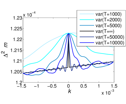
Figure 3: Variance of $m\left(t\right)=\langle\sigma_{i}^{z}\left(t\right)\rangle$ of as a function of the integrability breaking parameter $\kappa$. The quench parameters are ($\gamma=1$) $(\kappa_{0}=0,h_{0}=2.0),\,\to(\kappa_{1}=\kappa,\,h_{1}=2.7)$. The size is $L=8$. Data are obtained via full diagonalization of the Hamiltonian.

Finally, a compelling question is whether similar results generalize to more complex integrable models such as those integrable by Bethe Ansatz. To investigate this scenario we performed preliminary numerical simulations with the following Hamiltonian

$$H =\sum_{i=1}^{L}\left[\sigma_{i}^{x}\sigma_{i+1}^{x}+\sigma_{i}^{y}\sigma_{i+1}^{y}+\Delta\sigma_{i}^{z}\sigma_{i+1}^{z}+\right.$$

$$\left.\alpha\left(\sigma_{i}^{x}\sigma_{i+2}^{x}+\sigma_{i}^{y}\sigma_{i+2}^{y}+\Delta\sigma_{i}^{z}\sigma_{i+2}^{z}\right)\right],$$ (5)

with periodic boundary condition. At $\alpha=0$ the Hamiltonian is integrable by Bethe Ansatz. In our simulations we quenched from $\left(\Delta_{0},\alpha_{0}\right)$ to $\left(\Delta_{1},\alpha_{1}\right)$, and looked at the statistics of $\mathcal{A}\left(t\right)=\langle\sigma_{i}^{+}\sigma_{i+1}^{-}\left(t\right)\rangle+\mathrm{h.c.}$ as this is a quadratic observable in the fermionic setting. Our numerics shows that the fluctuations are smooth as $\alpha_{1}$ crosses the integrable point, which indicates that the non-resonant condition is satisfied (when restricted to the relevant subspace) also at the integrable point. This indeed has to be expected from the form of the many-body energies arising from the Bethe Ansatz . However it is still possible that a lack of rational independence of the many-body energies, for Bethe Ansatz integrable models, will show up in a non-analytic behavior of higher cumulants of $\mathcal{A}\left(t\right)$ as a function of the non-integrability parameter $\alpha$.

In figure 4 we plot the distribution function $P_{A}$ for $\mathcal{A}\left(t\right)$ for various quench experiment. At the integrable point the distribution looks qualitatively different from the distribution obtained at $\alpha_{1}\neq 0$. However further investigations are needed to ascertain whether the dependence of $P_{A}$ on $\alpha_{1}$ is analytic at the integrable point $\alpha_{1}=0$. A lack of analyticity would be a signature of a lack of rational independence of the many-body energies.

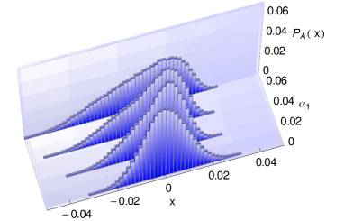
Figure 4: Full time statistics $P_{A}\left(x\right)$ for the observable $\mathcal{A}\left(t\right)=\langle\sigma_{i}^{+}\sigma_{i+1}^{-}\left(t\right)\rangle+\mathrm{h.c.}$ for the Hamiltonian Eq. (5). The quench parameters are $\left(\Delta_{0}=2,\,\alpha_{0}=1.7\right)\to\left(\Delta_{1}=1,\alpha_{1}=0,0.02,0.04,0.06\right)$ for a size $L=10$. At $\alpha_{1}=0$ the Hamiltonian is integrable by Bethe-Ansatz. Data are obtained with full diagonalization of Hamiltonian Eq. (5). For the time statistics, the observable $\mathcal{A}\left(t\right)$ has been computed at 200,000 random times distributed uniformly in $\left[0,T\right]$ with $T=100,000$.

VII Conclusions

In this paper we addressed the question of equilibration in quasi-free Fermi systems. The initial state is a general state while the evolution Hamiltonian as well as the observable are quadratic in the Fermi operators. While for general non-free systems the variance $\Delta\mathcal{A}^{2}$ is typically exponentially small in the volume, we find that in the quasi-free setting (for extensive observables) both the mean and the variance are proportional to the volume. This hints at the possibility of an underlying central limit theorem, a circumstance that we termed Gaussian equilibration. In this case the properly rescaled observable becomes Gaussian in the large $L$ limit, and in general the relative error satisfies $\Delta\mathcal{A}/\overline{\mathcal{A}}\sim 1/\sqrt{L}$. We proved Gaussian equilibration for the magnetization in the quantum XY model assuming rational independence of the one body energies and gave evidence for a class of observables/initial states evolving with a tight-binding model. In all cases Gaussian equilibration was confirmed by numerical simulations. The key insight is a mapping of the equilibration dynamics to a generalized classical XY model at infinite temperature. As a by product we obtain a quantum setting (initial state, Hamiltonian, and observable $A_{XY}$), such that the equilibration dynamics of $A_{XY}$ gives the solution of a classical XY model in $D$-dimension, and vice-versa.

A consequence of the above scenario –confirmed by numerical simulations– is that the variance $\Delta\mathcal{A}^{2}$ turns out to be discontinuous at the quasi-free point of an otherwise non-integrable Hamiltonian. This shows that the enhancement of the temporal fluctuations of $\Delta\mathcal{A}^{2}$ (for a quadratic observable $A$) may provide a universal and experimentally testable signature of integrability in the context of out of equilibrium dynamics, at least when integrable systems are identified with quadratic models.

Ultimately the origin of the exponential decrease of the signal to noise ratio illustrated in this paper lies in the exponential reduction of the effective phase space entailed by the quasi-free nature of our setup i.e., the many body space gets effectively replaced by the single particle one. A natural question for future research is whether a similar mechanism is at place for a more general class of integrable systems such as Bethe-Anstanz integrable models. Preliminary numerical results indicate that, in this case the variance is smooth and a possible non-analytic behavior at the integrable point must be sought in higher order cumulants.

LCV wishes to thank KITP for the kind hospitality. This research was partially supported by the ARO MURI under grant W911NF-11-1-0268 and by the National Science Foundation under Grant No. NSF PHY11-25915. PZ also acknowledges partial support by NSF grants No. PHY-969969 and No. PHY-803304.

References

- Kinoshita et al. (2006) T. Kinoshita, T. Wenger, and D. S. Weiss, Nature 440, 900 (2006).
- Calabrese and Cardy (2006) P. Calabrese and J. Cardy, Phys. Rev. Lett. 96, 136801 (2006).
- Hofferberth et al. (2007) S. Hofferberth, I. Lesanovsky, B. Fischer, T. Schumm, and J. Schmiedmayer, Nature 449, 324 (2007).
- Rigol et al. (2008) M. Rigol, V. Dunjko, and M. Olshanii, Nature 452, 854 (2008).
- Linden et al. (2009) N. Linden, S. Popescu, A. J. Short, and A. Winter, Phys. Rev. E 79, 061103 (2009).
- Campos Venuti and Zanardi (2010a) L. Campos Venuti and P. Zanardi, Phys. Rev. A 81, 022113 (2010a).
- Campos Venuti et al. (2011) L. Campos Venuti, N. T. Jacobson, S. Santra, and P. Zanardi, Phys. Rev. Lett. 107, 010403 (2011).
- Rigol et al. (2007) M. Rigol, V. Dunjko, V. Yurovsky, and M. Olshanii, Phys. Rev. Lett. 98, 050405 (2007).
- Kollath et al. (2007) C. Kollath, A. M. Läuchli, and E. Altman, Phys. Rev. Lett. 98, 180601 (2007).
- Barthel and Schollwöck (2008) T. Barthel and U. Schollwöck, Phys. Rev. Lett. 100, 100601 (2008).
- Campos Venuti and Zanardi (2010b) L. Campos Venuti and P. Zanardi, Phys. Rev. A 81, 032113 (2010b).
- Peschel (2003) I. Peschel, Journal of Physics A: Mathematical and General 36, L205 (2003).
- Lanford and Robinson (1972) O. E. Lanford and D. W. Robinson, Communications in Mathematical Physics (1965-1997) 24, 193 (1972).
- Cramer et al. (2008) M. Cramer, C. M. Dawson, J. Eisert, and T. J. Osborne, Phys. Rev. Lett. 100, 030602 (2008).
- Cramer and Eisert (2010) M. Cramer and J. Eisert, New Journal of Physics 12, 055020 (2010).
- Reimann (2008) P. Reimann, Phys. Rev. Lett. 101, 190403 (2008).
- Cassidy et al. (2011) A. C. Cassidy, C. W. Clark, and M. Rigol, Phys. Rev. Lett. 106, 140405 (2011).
- Gramsch and Rigol (2012) C. Gramsch and M. Rigol, arXiv:1206.3570 (2012).
- Lieb et al. (1961) E. Lieb, T. Schultz, and D. Mattis, Annals of Physics 16, 407 (1961).
- Barouch et al. (1970) E. Barouch, B. M. McCoy, and M. Dresden, Phys. Rev. A 2, 1075 (1970).
- Calabrese et al. (2012) P. Calabrese, F. H. L. Essler, and M. Fagotti, arXiv:1204.3911 (2012).
- Billingsley (2012) P. Billingsley, Probability and Measure (John Wiley & Sons, 2012).
- Tasaki (2010) H. Tasaki, arXiv:1003.5424 (2010).
- Mattis (1984) D. C. Mattis, Physics Letters A 104, 357 (1984).
- Beccaria et al. (2006) M. Beccaria, M. Campostrini, and A. Feo, Phys. Rev. B 73, 052402 (2006).