Integral field spectroscopy of a sample of nearby galaxies:

In this work we analyze the spectroscopic properties of a large number of H ii regions, $\sim$2600, located in 38 galaxies. The sample of galaxies has been assembled from the face-on spirals in the PINGS survey and a sample described in Mármol-Queraltó (2011, henceforth Paper I). All the galaxies were observed using Integral Field Spectroscopy with a similar setup, covering their optical extension up to $\sim$2.4 effective radii within a wavelength range from $\sim$3700 to $\sim$6900Å.

We develop a new automatic procedure to detect H ii regions, based on the contrast of the H$\alpha$ intensity maps extracted from the datacubes. Once detected, the procedure provides us with the integrated spectra of each individual segmented region. In total, we derive good quality spectroscopic information for $\sim$2600 independent H ii regions/complexes. This is by far the largest nearby 2-dimensional spectroscopic survey presented on this kind of regions up-to-date. Even more, our selection criteria and dataset guarantee that we cover the regions in an unbiased way, regarding the spatial sampling.

A well-tested automatic decoupling procedure has been applied to remove the underlying stellar population, deriving the main properties (intensity, dispersion and velocity) of the strongest emission lines in the considered wavelength range (covering from [O ii] $\lambda$3727 to [S ii] $\lambda$6731). A final catalogue of the spectroscopic properties of these regions has been created for each galaxy. Additional information regarding the morphology, spiral structure, gas kinematics, and surface brightness of the underlying stellar population has been included in each catalogue.

In the current study we focused on the understanding of the average properties of the H ii regions and their radial distributions. We found that, statistically, there is a significant change of the ionization conditions across the optical extent of the galaxies. The fraction of H ii regions located in the intermediate ionization range in a classical BPT diagram is larger for the central regions ($r<0.25r_{e}$), than in the outer ones. This is somehow expected, if the origin of this shift is due to the contamination of non-starforming ionization sources (e.g., AGN, Shocks, post-AGB stars, etc.), that occur more frequently in the center of the galaxies.

We find that the gas-phase oxygen abundance and the H$\alpha$ equivalent width present negative and positive gradient, respectively. The distribution of slopes is statistically compatible with a random Gaussian distribution around the mean value, if the radial distances are measured in units of the respective effective radius. No difference in the slope is found for galaxies of different morphologies: barred/non-barred, grand-design/flocculent. Therefore, the effective radius is a universal scale length for gradients in the evolution of galaxies.

Other properties have a larger variance across each object, and galaxy by galaxy (like the electron density), without a clear characteristic value, or they are well described by the average value either galaxy by galaxy or among the different galaxies (like the dust attenuation).

1 Introduction

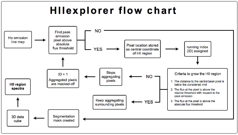
Figure 1: Flow chart of HIIexplorer, the algorithm developed to select, segregate, and extract the spectra of the individual H ii regions for the analyzed galaxies.

Nebular emission lines from bright-individual H ii regions have been, historically, the main tool at our disposal for the direct measurement of the gas-phase abundance at discrete spatial positions in galaxies. A good observational understanding of the distribution of element abundances across the surface of nearby galaxies is necessary to place constrains on theories of galactic chemical evolution. The same information is crucial to derive accurate star formation histories of and obtain information on the stellar nucleosynthesis in normal spiral galaxies.

Several factors dictate the chemical evolution in a galaxy, including the primordial composition, the content and distribution of molecular and neutral gas, the star formation history (SFH), feedback, the transport and mixing of gas, the initial mass function (IMF), etc (e.g. López-Sánchez, 2010; López-Sánchez & Esteban, 2010, and references therein). All these ingredients contribute through a complex process to the evolutionary histories of the stars and the galaxies in general. Accurate measurements of the present chemical abundance constrain the different possible evolutionary scenarios, and thus the importance of determining the elemental composition in a global approach, among different galaxy types.

Table 1: Main properties of the analyzed galaxies

Name	RA	Dec	Class	$z$	B	B-V	mod	MB	vrot	incl	PA	re	Type	Arms
(1)	(2)	(3)	(4)	(5)	(6)	(7)	(8)	(9 )	(10 )	(11)	(12)	(13)	(14)	(15)
2MASXJ1319+53	13:19:35.9	+53:30:09.8	Sb	0.0248	15.92	0.72	35.3	-19.3	51	28.0	55	9.7	L	NC
CGCG 071-096	13:00:33.2	+10:07:47.8	Sb(r)	0.0239	14.69	0.79	35.1	-20.5	125	45.0	220	10.7	I/L	NC
CGCG 148-006	07:44:57.4	+28:55:39.0	Sc	0.0234	15.16	0.75	35.1	-19.9	180	40.5	250	10.3	L	NC
CGCG 293-023	02:30:21.5	+56:47:29.5	SBb	0.0156	15.51	0.99	34.3	-18.8	325	19.6	100	6.9	L	NC
CGCG 430-046	23:00:46.2	+13:37:07.9	Sc	0.0243	14.49	0.86	35.1	-20.7	168	42.1	160	11.0	L	NC
IC 2204	07:41:18.1	+34:13:55.9	Sab	0.0155	15.71	0.93	34.2	-18.5	49	24.1	58	15.5	I/E	AGN
MRK 1477	13:16:14.7	+41:29:40.1	SBa(r)	0.0207	14.83	0.47	34.9	-20.0	144	59.0	100	7.9	L	NC
NGC 99	00:23:59.5	+15:46:13.7	Sc	0.0177	13.71	0.62	34.5	-20.7	79	33.7	40	19.9	L	NC
NGC 3820	11:42:04.9	+10:23:03.3	Sbc	0.0203	14.97	0.95	34.8	-19.8	95	41.6	205	8.5	L	NC
NGC 4109	12:06:51.1	+42:59:44.3	Sa	0.0235	14.79	0.98	35.1	-20.7	132	44.0	220	7.5	E	NC
NGC 7570	23:16:44.7	+13:28:58.8	Sa	0.0157	13.40	0.81	34.2	-20.8	81	65.7	130	21.6	I/E	NC
UGC 74	00:08:44.7	+04:36:45.1	Sc	0.0131	13.51	0.85	33.8	-20.3	135	38.3	130	24.6	L	(s)
UGC 233	00:24:42.7	+14:49:28.8	SBbcD	0.0176	14.35	0.62	34.4	-20.1	161	4.1	150	6.9	L	NC
UGC 463	00:43:32.4	+14:20:33.2	SABc	0.0148	12.93	0.85	34.1	-21.1	134	40.0	40	20.6	L	(s)
UGC 1081	01:30:46.6	+21:26:25.5	Sc	0.0104	13.54	0.83	33.3	-19.8	82	22.0	130	31.2	L	(s)
UGC 1087	01:31:26.6	+14:16:39.0	Sc	0.0149	14.56	0.69	34.1	-19.5	74	21.6	60	19.1	L	(s)
UGC 1529	02:02:31.0	+11:05:35.1	Sc	0.0155	13.67	1.01	34.2	-20.5	166	45.4	132	17.8	L	(s)
UGC 1635	02:08:27.7	+06:23:41.7	Sbc	0.0115	14.29	0.96	33.5	-19.2	71	32.6	220	24.0	L	NC
UGC 1862	02:24:24.8	-02:09:44.5	SABc	0.0046	13.41	0.83	31.5	-18.1	68	49.4	25	67.5	L	(s)
UGC 3091	04:33:56.1	+01:06:49.5	SABc	0.0184	14.67	0.88	34.5	-19.8	236	39.1	100	5.2	L	(s)
UGC 3140	04:42:54.9	+00:37:06.9	Sc	0.0154	12.84	0.97	34.1	-21.3	68	31.2	40	16.7	L	AC09
UGC 3701	07:11:42.7	+72:10:09.5	Sc	0.0097	14.76	0.87	33.3	-18.5	76	0.0	85	22.6	L	(s)
UGC 4036	07:51:54.7	+73:00:56.5	SABb	0.0116	12.81	0.98	33.7	-20.9	73	24.6	125	30.6	L	AC12
UGC 4107	07:57:01.9	+49:34:02.5	Sc	0.0117	13.64	1.06	33.7	-20.9	84	19.7	40	19.2	L	(s)
UGC 5100	09:34:38.6	+05:50:29.9	SBb	0.0184	14.15	1.02	34.5	-20.4	326	69.8	100	11.1	I/L	(s)
UGC 6410	11:24:05.9	+45:48:39.9	SABc	0.0187	14.32	0.78	34.7	-20.3	185	44.2	100	16.5	L	NC
UGC 9837	15:23:51.7	+58:03:10.6	SABc	0.0089	13.65	0.57	33.2	-19.5	90	23.2	145	30.8	L	(s)
UGC 9965	15:40:06.7	+20:40:50.2	Sc	0.0151	14.06	0.72	34.2	-20.1	137	22.4	73	17.8	L	(s)
UGC 11318	18:39:12.2	+55:38:30.5	Sbc	0.0196	13.27	0.72	34.8	-21.5	77	21.0	72	28.7	I/L	(s)
UGC 12250	22:55:35.9	+12:47:25.1	SBb	0.0242	13.78	1.04	35.1	-21.4	435	55.8	73	26.2	I/L	NC
UGC 12391	23:08:57.2	+12:02:52.9	SABc	0.0163	13.26	0.77	34.3	-21.0	112	27.2	40	24.9	L	AC2
PINGS galaxies
NGC 628	01:36:41.7	+15:47:01.0	Sc	0.00219	9.35	0.56	29.7	-20.7	101	34.9	100	122.2	L	AC9
NGC 1058	02:43:30.0	+37:20:29.0	Sc	0.00173	11.24	0.62	29.9	-18.5	115	19.6	100	45.0	L	AC3
NGC 1637	04:41:28.2	-02:51:29.0	Sc	0.00239	11.27	0.64	30.4	-18.5	114	31.1	131	48.7	L	AC5
NGC 3184	10:18:16.8	+41:25:27.0	SABc	0.00194	10.31	0.58	30.2	-20.0	108	24.2	117	109.3	L	AC9
NGC 3310	10:38:45.8	+53:30:12.0	SABb	0.00331	11.15	0.35	31.2	-20.1	158	31.2	237	37.9	L	AC1
NGC 4625	12:41:52.7	+41:16:26.0	SABm	0.00203	12.73	0.57	30.5	-17.8	105	46.1	73	25.5	L	AC4
NGC 5474	14:05:01.6	+53:39:44.0	Sc	0.00098	11.11	0.49	29.2	-18.0	40	50.2	100	58.5	L	AC2

Notes: (1): Galaxy name from NED, the NASA$/$IPAC Extragalactic Database (http://nedwww.ipac.caltech.edu/). (2)-(3): Right ascension and declination coordinates in J2000 Equinox, expressed in units of RA (hh mm ss) and Dec (dd mm ss). (4): Morphologycal types obtained from NED and Hyperleda (Paturel et al., 2003, , http://leda.univ-lyon1.fr) following the Third Reference Catalogue of Bright Galaxies (RC3) classification (Corwin et al., 1994, , http://vizier.u-strasbg.fr/viz-bin/VizieR?-source=VII/155). (5): Redshift values from NED. (6): Dust corrected B-band magnitude calculated from Hyperleda. (7): (B-V) colors obtained from Hyperleda expressed in magnitudes. (8) Distance modulus extracted from Hyperleda. (9) M_B: Dust corrected B magnitude extracted from Hyperleda. (10): Rotation velocity in units of km s^-1 from NED. (11): Absolute value of the inclination angle derived from Hyperleda. (12): Position angle values from our own analysis as described in the text, units are degrees. (13): Effective radius from this work, units are arcsecs. (14): Disks classification (L: Late, E: early, I: intermediate) according to the Laurikainen et al. (2010) criteria. (15): Spiral arm classification following the classes proposed by Elmegreen & Elmegreen (1987), when not avalaible we use the RC3 classification.

Previous spectroscopic studies have unveiled some aspects of the complex processes at play between the chemical abundances of galaxies and their physical properties. Although these studies have been successful in determining important relationships, scaling laws and systematic patterns (e.g. luminosity-metallicity, mass-metallicity, and surface brightness vs. metallicity relations Lequeux et al. 1979; Skillman 1989; Vila-Costas & Edmunds 1992; Zaritsky et al. 1994; Tremonti et al. 2004; effective yield vs. luminosity and circular velocity relations Garnett 2002; abundance gradients and the effective radius of disks Diaz 1989; systematic differences in the gas-phase abundance gradients between normal and barred spirals Zaritsky et al. 1994; Martin & Roy 1994; characteristic vs. integrated abundances Moustakas & Kennicutt 2006; etc.), they have been limited by statistics, either in the number of observed H ii regions or in the coverage of these regions within the galaxy surface.

Hitherto, most studies devoted to the chemical abundance of extragalactic nebulae have only been able to measure the first two moments of the abundance distribution: the mean metal abundances of discs and their radial gradients. Indeed, most of the observations targeting nebular emission have been made with single-aperture or long-slit spectrographs, resulting in a small number of galaxies studied in detail, a small number of H ii regions studied per galaxy, and a limited coverage of these regions within the galaxy surface. The advent of Multi-Object Spectrometers and Integral Field Spectroscopy (IFS) instruments with large fields of view now offers us the opportunity to undertake a new generation of emission-line surveys, based on samples of scores to hundreds of H ii regions and full two-dimensional (2D) coverage of the discs of nearby spiral galaxies.

In the last few years we started a major observational program to understand the statistical properties of H ii regions, and to unveil the nature of the reported physical relations, using IFS. This program was initiated with the PINGS survey (Rosales-Ortega et al. 2010), which acquired IFS mosaic data of a number of medium size nearby galaxies. In Sánchez et al. (2011) and Rosales-Ortega et al. (2011), we studied in detail the ionized gas and H ii regions of the largest galaxy in the sample (NGC 628). We then continued the acquisition of IFS data for a larger sample of visually classified face-on spiral galaxies (Mármol-Queraltó et al., 2011, hereafter Paper I), as part of the feasibility studies for the CALIFA survey (Sánchez et al., 2012). The spatially resolved properties of a typical galaxy in this sample, UGC9837, was presented by Viironen et al. (2012). Face-on galaxies are more suitable to study the spatial distribution of the properties of H ii regions: (i) they are identified and segregated more easily; (ii) their spatial distribution is less prompt to the errors induced by inclination effects; (iii) they are less affected by dust extinction along the line of sight within the galaxy and (iv) it is more easy to identify their association with a particular spiral arm.

In this article we focus on the study of the properties of the H ii regions for the face-on spiral galaxies observed so far. In Sect. 2 we summarize the main properties of the analyzed galaxies. In Sect. 3 we present the automatic algorithm developed to detect, segregate and extract the integrated spectra of the different H ii regions within a datacube; a comparison between the results derived with this method and those provided with other published ones is shown in Sect. 4. In Sect. 5 we describe an analytical method to define the presence and location of spiral arms within a galaxy. The method has been tested and used to associate the detected H ii regions to different spiral arms and/or to the intra-arm region. The main spectroscopic properties of the catalogued H ii regions and the morphological structure of each galaxy are described in Sect. 6.1.1 and 6.1.2. The main results of our analysis are included in Sect. 7, where we describe the statistical properties of the H ii regions (Sect. 7.1), and their radial gradients (Sect. 7.2). The conclusions of this study are presented in Sect. 8. In the appendix, the publicly accessible catalogues of the properties derived for the analyzed H II regions are described in Sect. A, and an empirical correction to decontaminate the [N II] emission on narrow-band H$\alpha$ images is proposed in Sect. B.

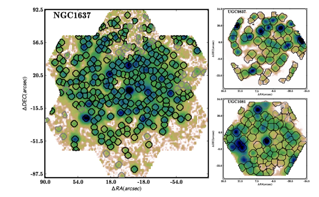
Figure 2: IFS-based H$\alpha$ maps derived for three representative galaxies of the sample (color images), together with the detected H ii regions shown as black segmented contours. The regions plotted in grey e have been removed from the final catalogue after a sanity-check due to low S/N, quality problems in the extracted spectra, and/or affected by vignetting effects.

2 Sample of galaxies

Table 1 lists the sample of galaxies analyzed in the current study, including for each object, its name, central coordinates, morphological classification, redshift, and some additional information that we will describe later. The sample of galaxies has been selected from two available datasets: (1) the IFS survey of nearby galaxies described in Paper I, which comprises $\sim$85% of the galaxies analyzed here, and (2) galaxies selected from the PINGS survey (Rosales-Ortega et al., 2010), accounting for the remaining $\sim$15% of the galaxies. In both cases we selected visually classified face-on galaxies, with a relatively unperturbed spiral structure.

The sample is dominated by late-type spirals (31 out of 38), according to the classification criteria by Laurikainen et al. (2010), shown in Table 1. Therefore, we lack the statistics required to analyze possible differences in the properties of H ii regions between late/early-type spirals. About 40% of the galaxies show evidence of a bar (based on its visual classification listed in Table 1), although only in a few of them this feature clearly dominates the morphology of the galaxy (e.g. UGC 5100). Regarding the structure of their spiral arms, the sample includes a mix of grand-design spirals (e.g. NGC 628), or clearly flocculent ones (e.g., UGC 9837 Viironen et al., 2012). Although it is by no means a statistically well defined sample, we consider that it is representative of the average population of spiral galaxies in the local Universe.

Both sub-samples of galaxies were observed using similar techniques (IFS), using the same instrument (PMAS in the PPAK configuration, Roth et al., 2005; Kelz et al., 2006), covering a similar wavelength range ($\sim$3700-6900Å), with similar resolutions and integration times. The data reduction was performed using the same procedure (R3D, Sánchez, 2006a), as described in Paper I and Rosales-Ortega et al. (2010). The main difference is that for the first sample a single pointing strategy using a dithering scheme was applied, while for the largest galaxies of the PINGS survey, a mosaic comprising different pointings was required. This is due to the differences in projected size, considering the different redshift range of both samples: for the first one corresponds to $\sim$0.01-0.025, while for the second one corresponds to $\sim$0.001-0.003. Therefore, in both cases the covered field-of-view (FoV) corresponds to a similar optical size, $\sim$2 effective radii, in general (the effective radius is classically defined as the radius at which one half of the total light of the system is emitted).

The observational setups allow us to cover the optical wavelength range, sampling many of the most important emission lines for H ii regions, from [O ii] $\lambda$3727 to [S ii] $\lambda$6731. Details on the observing strategy, setups, reduction and main characteristics of the dataset are described in Paper I and Rosales-Ortega et al. (2010). The final dataset comprises 38 individual datacubes, one per galaxy, with a final spatial sampling of 1$\arcsec$/pixel for most of the galaxies. The datacubes were created using the interpolation scheme described in Sánchez et al. (2012), developed for the CALIFA survey. Despite of the original fiber size (2.7$\arcsec$/fiber), the three pointing dithering scheme allows to increase slightly the final resolution. The selected offsets, with values corresponding to a fraction of the fiber-size, allows to cover the gaps between adjacent fibers too. In average natural seeing conditions of $\sim$1$\arcsec$ (Sánchez et al., 2007a), this technique allows to provide a final spatial resolution of FWHM$\sim$2$\arcsec$ for this instrument (Sánchez et al., 2007b). The size of the spaxel was selected as the largest convient pixel to the sample this resolution element, 2 pixels per FWHM, i.e., 1$\arcsec$/pixel. Due to the large size of the IFS mosaics of NGC 628 and NGC 3184, the two largest galaxies observed with PINGS, and the fact that they were not observed using a dithering scheme for all the pointings , we set the spatial sampling to 2$\arcsec$/pixels. In this case, the final resolution is larger than the original size of the fiber, due to the interpolation kernel. A rough estimation indicate that the final spatial resolution is FWHM$\sim$3.5-4$\arcsec$.

On average the physical spatial sampling ranges between a few hundreds of parsecs (for the nearest galaxies) to almost 1 kpc (for the more distant ones). To derive this physical scale it is required to adopt a certain distance modulus. Consistently with values reported in Table 1, we adopted the distance modulus provided by Hyperleda, $mod$, defined as:

$$mod=5\log(D_{L})+25$$ (1)

and $D_{L}$ is the luminosity distance in Mpc. The derived scale can be compared to the physical diameter of a well-known H ii region in our Galaxy, i.e. the Orion nebula (D$\sim$8 pc), or to the extent of those which are considered prototypes of extragalactic giant H ii regions, such as 30 Doradus (D$\sim$200 pc), NGC 604 (D$\sim$460 pc) or NGC 5471 (D$\sim$1 kpc) as reported by Oey et al. (2003) and García-Benito et al. (2011). Thus, given the undersampling in the physical size of the H ii regions in our data, we cannot use it to derive direct estimates of the optical extension of these regions. In other aspects, like the depth, covered extension of the galaxy, projected resolution and wavelength coverage, the data provided by both samples are very similar.

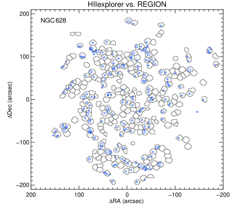
Figure 3: Comparison between the H ii region catalogue of NGC 628 obtained by HIIexplorer using IFS data (grey contours, 286 regions) and the (modified) Fathi et al. (2007) catalogue obtained with Region using a traditional H$\alpha$ narrow-band image (blue circles, 180 regions). Only those regions within the FoV of the IFS data have been considered.

Table 2: Detected HII regions within our sample.

Galaxy	NHII	N${}_{\rm HII}^{*}$	NHβ	FHα	$\sigma_{\rm H\alpha}$	rHII	$\sigma_{\rm r}$
(1)	(2)	(3)	(4)	(5)	(6)	(7)	(8)
2MASXJ1319+53	19	18	14	1.25	0.93	16.48	1.42
CGCG 071-096	27	27	22	1.65	1.70	15.38	1.45
CGCG 148-006	40	29	26	1.52	1.33	14.15	1.37
CGCG 293-023	19	18	8	1.36	1.25	10.29	1.02
CGCG 430-046	33	24	23	1.83	1.58	15.33	0.96
IC 2204	59	59	30	1.57	1.74	10.17	0.95
MRK 1477	8	8	7	2.46	2.77	14.52	0.68
NGC 99	63	63	62	1.77	1.89	11.43	1.01
NGC 3820	18	16	15	1.62	1.47	12.56	1.04
NGC 4109	15	15	15	1.75	1.75	15.68	0.85
NGC 7570	50	50	27	1.65	2.04	10.25	0.78
UGC 74	91	78	65	1.28	1.03	8.01	0.79
UGC 233	49	49	26	1.89	2.02	10.99	1.20
UGC 463	85	83	80	1.79	1.77	9.14	0.87
UGC 1081	90	87	81	1.29	1.32	6.25	0.92
UGC 1087	82	81	76	1.21	0.92	8.91	0.92
UGC 1529	116	77	52	1.65	1.34	9.19	0.94
UGC 1635	85	84	84	0.91	0.54	6.64	0.72
UGC 1862	56	55	53	1.19	1.06	2.69	0.20
UGC 3091	68	66	61	1.09	0.73	11.08	1.18
UGC 3140	87	86	86	1.62	1.51	9.28	0.96
UGC 3701	80	69	53	1.46	1.24	6.55	0.51
UGC 4036	104	104	79	1.67	1.73	7.48	0.84
UGC 4107	68	68	61	1.45	1.41	7.65	0.68
UGC 5100	28	28	20	1.61	1.71	11.89	1.08
UGC 6410	62	61	60	1.33	1.20	11.98	1.02
UGC 9837	65	64	64	1.37	1.41	5.95	0.85
UGC 9965	68	67	65	1.55	1.45	9.81	0.91
UGC 11318	76	75	62	1.56	1.41	12.53	1.65
UGC 12250	81	41	21	1.46	1.12	14.71	1.06
UGC 12391	91	84	71	1.54	1.45	10.21	0.89
PINGS
NGC 628	373	366	282	2.70	2.89	2.87	0.33
NGC 1058	331	258	179	2.69	2.83	1.47	0.11
NGC 1637	297	297	251	2.46	2.89	1.35	0.14
NGC 3184	169	169	124	2.86	2.94	3.31	0.36
NGC 3310	203	130	121	3.93	4.25	2.53	0.33
NGC 4625	66	49	46	3.10	3.11	1.83	0.25
NGC 5474	122	121	95	2.74	2.91	1.13	0.14

Notes: (1) Name of the galaxy used along this article; (2) number of detected HII regions; (3) number of HII regions with good quality spectra, as described in the text; (4) number of HII regions with H$\beta$ emission line detected at 3$\sigma$ significance; (5) median value of the H$\alpha$ intensity derived from the narrow-band images in 10^-16 erg s^-1 cm^-2; (6) standard deviation of the H$\alpha$ intensity in the same; (7) median value of the estimated radii of the HII regions in units of 100 pc (we need to note that the size derived by HIIexplorer is an ill-defined parameter for our dataset) ; (8) standard deviation of the previous estimated radii, in the same units.

3 Extraction of the H ii regions

The segregation of H ii regions and the extraction of the corresponding spectra is performed using a semi-automatic procedure, named HIIexplorer. The procedure is based on some basic assumptions: (a) H ii regions are peaky/isolated structures with a strong ionized gas emission, clearly above the continuum emission and the average ionized gas emission across the galaxy; (b) H ii regions have a typical physical size of about a hundred or a few hundreds of parsecs (e.g. Gonzalez Delgado & Perez, 1997; Lopez et al., 2011; Oey et al., 2003), which corresponds to a typical projected size at the distance of the galaxies of a few arcsec.

The algorithm requires a set of input parameters: (i) a line emission map, with the same world-coordinate system (WCS) and resolution as the input datacube (preferentially an H$\alpha$ emission line map); (ii) a flux intensity threshold for the peak emission of each H ii region; (iii) a maximum distance to the peak location for a pixel associated with each H ii region; (iv) a relative threshold with respect to this peak emission of the minimum intensity of each H ii region; (v) an absolute threshold of the minimum intensity corresponding to each H ii region. All these parameters can be derived from either a visual inspection and/or a statistical analysis of the H$\alpha$ emission line map. The algorithm produces as an output a segmentation FITS file describing the pixels associated to each H ii region, designated with a running index starting with 1 (e.g. the primary H ii region ID in this article), with the zero reserved to areas not associated with any H ii region (i.e. regions free of emission or below the absolute threshold described above).

The segregation algorithm is based on a simple iterative procedure, summarized in the flow chart shown in Fig. 1. As a first step the algorithm looks for the brightest pixel within the emission line map. Its location is stored as the peak/central coordinate of a new H ii region, associated with a certain running index (ID number). After this, the adjacent pixels are aggregated to this H ii region if all of the following criteria are fulfilled: (i) the distance to the central/peak pixel is below the selected limit; (ii) the flux at the pixel is above the relative threshold with respect to the peak emission; (iii) the flux at the pixel is above the absolute flux threshold described before. Whenever any of these criteria are not fulfilled the aggregation procedure stops, the ID number is increased by one, all the aggregated pixels are masked-off, and the peak-identification procedure is repeated. The overall procedure stops whenever no new peak is detected above the selected peak-intensity threshold.

The outcome of the procedure is illustrated in Fig. 2 where we show: (i) the input emission line map, in this case the H$\alpha$ map corresponding to a set of galaxies and (ii) the corresponding derived segmentation map. Despite the simplicity of the described algorithm it is clearly seen that (1) it is able to detect all the H ii regions that can be identified by eye, and (2) it produces a reliable segmentation map. The black segmented areas indicate those regions with good quality spectra, while the grey ones indicate those with poor extracted spectra. The actual procedure to detect and reject those ones is described later. In addition, the procedure provides with a mask where all the H ii regions are flagged out. This mask is important to define the areas where it is possible to study the diffuse gas emission.

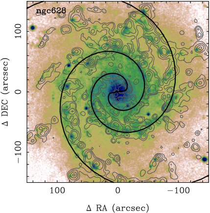
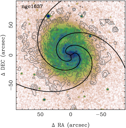
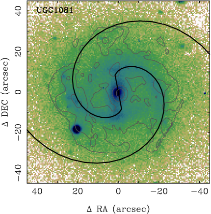
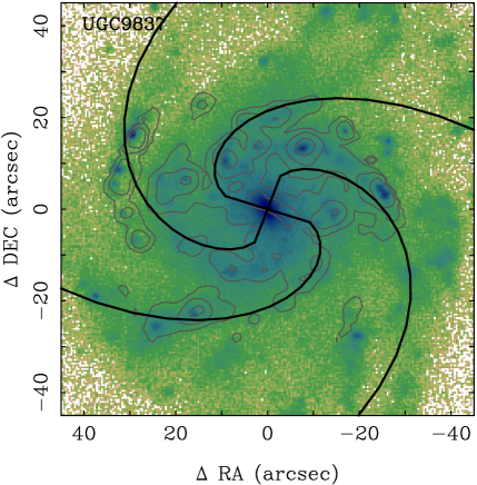
Figure 4: Continuum map of four representative galaxies of the full sample (color images), together with a contour plot of the H$\alpha$ intensity map (both in arbitrary units). The solid lines show the location of the identified spiral arms as a result of the fitting procedure. Left side panels show galaxies with clearly defined spiral arms, while right side panels show galaxies with poorly identified ones.

There are other publicly accessible packages for the automatic selection/segregation of H ii regions in the literature (e.g. HIIphot, Thilker et al. 2000; Region, Fathi et al. 2007), that in principle could be adapted for the main purpose of the current study. However, these packages are strongly focused on the analysis of narrow-band images, of much higher spatial resolution, where the H ii regions are clearly resolved. In some cases the procedure requires a detailed knowledge of the observational procedure (number of frames co-added, ADU of the CCD, etc.). For example, HIIphot uses object recognition techniques to make a first guess at the shapes of all sources and then allows for departure from such idealized seeds through an iterative growing procedure. In essence, this algorithm is similar to the one used by SExtractor (Bertin & Arnouts, 1996), for the detection and segregation of galaxies in crowed fields. We experimented with these packages before developing our own code, but we did not get any optimal solution. The main reasons were that (1) our data have a much coarser resolution than the one provided by narrow-band imaging (even from ground-based telescopes); (2) reconstructed IFU map have a strong cross-correlated noise among nearby interpolated pixels and (3) none of the preceding codes provide a final segmentation map usable to extract the integrated spectra of the H ii regions from the datacubes in a convenient way.

We experimented with the use of HIIexplorer on a H$\alpha$ narrow-band image provided by the SINGS legacy survey for NGC 628 (Kennicutt et al., 2003). A visual inspection of the selected regions with those shown by Thilker et al. (2000), indicates that although we detect similar regions, HIIexplorer tends to define regions of mostly equal size. This is expected, since for the spatial resolution the maximum size allowed for each region is reached before that imposed by the ratio of local to peak intensity. Our code was never meant to provide a particularly reliable measure of the projected size, as in our data this parameter is ill-defined. Specifically, H ii regions can be significantly smaller than the resolution element size. In Sect. 4 we present a quantitative comparison with methods available in the literature.

Once tested the procedure, we applied it to our IFS data. First, we create a H$\alpha$ intensity map for each object by co-adding the flux intensity within a square-shaped simulated filter centered at the wavelength of H$\alpha$ (6563Å), with a width of 60 Å. The adjacent continuum for each pixel was derived by averaging the flux intensity within two similar bands red- and blue-shifted 100 Å from the center of the initial one. This continuum intensity is then subtracted from the H$\alpha$ intensity to derive a continuum-subtracted emission line map. The central wavelength of all these bands has been shifted to the observed frame taking into account the redshift of the object. The separations between the filters and the filter widths are large enough to avoid any possible error in the derivation of the H$\alpha$ intensity map due to kinematic shifts.

Table 3: Derived parameters for the modelled spiral arms.

Galaxy	QF	NA	A	B	C
(1)	(2)	(3)	(4)
2MASXJ1319+53	1	2	10	3.0	11.0
CGCG 071-096	1	2	26	1.0	6.7
CGCG 148-006	1	2	9	1.0	6.1
CGCG 293-023	0	2	27	1.0	7.7
CGCG 430-046	0	2	6	1.0	4.7
IC 2204	1	2	18	1.5	7.7
MRK 1477	0	2	26	0.2	1.6
NGC 99	1	2	20	1.0	4.5
NGC 3820	0	4	17	1.0	2.6
NGC 4109	0	2	8	1.0	5.0
NGC 7570	1	2	50	0.9	9.0
UGC 74	1	2	22	1.0	4.2
UGC 233	1	2	22	1.0	6.7
UGC 463	0	3	26	1.0	3.6
UGC 1081	1	2	36	1.0	5.3
UGC 1087	0	2	20	1.0	6.0
UGC 1529	0	2	13	1.0	4.2
UGC 1635	0	2	16	1.0	5.2
UGC 1862	1	2	56	1.0	7.7
UGC 3091	0	5	29	1.0	1.4
UGC 3140	1	2	26	1.0	4.7
UGC 3701	0	2	20	1.0	2.9
UGC 4036	1	2	27	1.0	3.1
UGC 4107	1	3	20	1.0	4.2
UGC 5100	1	2	55	2.0	16.6
UGC 6410	1	2	27	1.0	6.7
UGC 9837	0	4	27	1.0	2.6
UGC 9965	0	2	29	1.0	5.3
UGC 11318	1	2	25	1.0	5.8
UGC 12250	1	2	17	1.0	6.2
UGC 12391	0	2	30	1.0	4.5
NGC 628	1	2	58	5.0	44.0
NGC 1058	0	2	50	1.0	4.1
NGC 1637	0	3	26	15.0	54.0
NGC 3184	1	2	170	15.0	70.0
NGC 3310	1	2	14	1.1	2.5
NGC 4625	0	1	23	1.0	9.7
NGC 5474	0	2	60	1.0	7.6

Notes: (1) Galaxy name used along this article; (2) quality flag of the analysis of the spiral arms: 1 = well defined arms, 0 = arms not well-defined; (3) number of arms detected with our modelling; (4) A, B, C parameter of the spiral model, described in Sect. 5, equation 2 by Ringermacher & Mead (2009). $A$ is in units of arcsec, $B$ is a dimensionless parameter, and $C$ is in units of radians^-1.

However, this H$\alpha$ intensity map is contaminated with the adjacent [N ii] emission lines, and it is not corrected for the emission of the underlying stellar population (see AppendixB for a discussion on the topic). A cleaner H$\alpha$ emission map can be derived using emission-line/stellar population decoupling procedures (e.g., Rosales-Ortega et al., 2010; Sánchez et al., 2011; Mármol-Queraltó et al., 2011; Sánchez et al., 2012). This allow us to recover much fainter emission line regions on top of underlying strong absorption features. However, in most cases these emission line regions do not correspond with classical H ii regions and are associated with other ionization processes (e.g. Kehrig et al., 2012, , and references there in). On the other hand, the adopted procedure resembles as much as possible the classical procedure used to detect H ii regions, which will allow us to make a better comparison with previous results.

As the main goal of the current study is to extract the spectroscopic properties of the H ii regions, we applied HIIexplorer adopting the following input parameters for all the galaxies: (i) a minimum flux density for the peak intensity of an H ii region of 2 10^-17 erg s^-1 cm^-2 arcsec^-1; (ii) a minimum relative flux to the peak intensity for associated pixels corresponding to the same H ii region of 10% and (iii) a maximum distance to the location of the peak of 3.5$\arcsec$ (7$\arcsec$ for NGC 628 and NGC 3184). The maximum distance was selected using and iterative process, maximizing the number of detections when compared with a visual inspection, and do not allow to segment clearly single H ii regions. Then, we extracted a single spectrum for each region by co-adding all the spectra in the original cubes with the same identification index (ID) in the the derived segmentation map. The final spectra are stored in the so-called row-stacked spectra (RSS) format Sánchez et al. (2004), which comprises a 2D spectral image, with the spectrum corresponding to each H ii region order by rows (each one corresponding to the considered ID), and an associated position table which records the barycenter of each H ii region (based on the H$\alpha$ intensity). This format allows us to visualize individual spectra of H ii regions and their spatial distribution using standard techniques (e.g., E3D, Sánchez et al., 2004). The ID is a unique identification index that will be used to identify the H ii regions hereafter (including the tables, figures and on-line material).

Table 2 summarizes the results from this analysis. It shows, for each galaxy, the number of H ii regions detected, the number of regions with good quality extracted spectra, the median H$\alpha$ flux intensity as directly measured from the IFS-based narrow-band image, and its standard deviation. Due to the different redshift range, there is a wide variance in the median flux intensity of the H$\alpha$ emission, much larger than the absolute luminosity as we will describe later. Since we are selecting H ii regions which physical size is slightly smaller than our typical resolution element, this implies that we are actually not aggregating a large number of real H ii regions in each detected complex. Our comparisons with higher resolution narrow-band images confirms this suspicion. Finally, we have included in the table the median radius of the regions, defined as R=$\sqrt{A/\pi}$, where A is the area within a region (Rosales-Ortega et al. 2011). We should state clearly here that the physical scale is an ill-defined parameter in our survey, due to two reasons: 1) the coarse spatial sampling compared to the expected size of H ii regions, these can be significantly smaller than the resolution element size and 2) the adopted procedure to detect and segregate the regions, namely the introduction of an angular upper size limit to the continuous emission region. Only for the galaxies at lower redshift, the sizes of the H ii regions are of the order of the expected one, i.e. $\sim$100 pc.

In practice, our segregated H ii regions may comprise several classical ones, in particular for the more distant galaxies. Detailed simulations on the effect of resolution loss have shown us that on average each selected region at $z\sim$0.02 may comprise 1-3 H ii regions from the ones selected from low redshift galaxies, $z\sim$0.002 (Mast et al., in prep.). Following Lopez et al. (2011), the considered H ii regions would have a size of a few to several hundreds of parsecs, based on their H$\alpha$ luminosity, detailed in Section 7.1, Table 7. Thererefore, the results from the simulations are expected, due to the typical size of an extragalactic H ii region and the lose of physical resolution at the higher redshifts. i.e. we are selecting H ii-regions and/or H ii aggregations (note that throughout this paper we will refer indistinctively to these segmented regions as H ii regions). Therefore, our results are not useful to analyze additive/integrated properties on individual H ii regions, like the H$\alpha$ luminosity function, but are perfectly suited for the study of line ratios, chemical abundances and ionization conditions.

In total, we have detected 3107 H ii regions, 2573 of them with good spectroscopic information. To our knowledge this is by far the largest 2-dimensional, nearby spectroscopic H ii region survey ever accomplished.

4 Comparisons with previous selection methods to detect H ii regions

In order to assess quantitatively the degree of segmentation provided by HIIexplorer with respect to other traditional H ii region catalogues generators, we performed a comparison between the H ii region catalogues of NGC 628, NGC 3184 and NGC 5474 obtained with HIIexplorer and those reported in the literature.

For NGC 628 we used the H$\alpha$ image extracted from the IFS data with a resolution of 2 arcsec/pixel and a FoV of $\sim 6$ arcmin, and the one produced by the REGION software in Fathi et al. (2007) (hereafter Fa07), obtained from a narrow-band H$\alpha$ image with a resolution of 0.33 arcsec/pixel and a FoV of $\sim 11$ arcmin. Similar comparisons could be performed with any other package created to segregate H ii regions (e.g. HIIPhot, Thilker et al., 2000). We selected this one because Fa07 provided publicly accessible catalogues.

The full Fa07 catalogue has 376 regions of which 299 are within the FoV of our IFS data. However, the public Fa07 catalogue reports only the position and the full-width at half maximum (FWHM) of each H ii region, not the actual shape obtained by the software, and this leads to significant overlaps when the REGION catalogue is plotted over the galaxy image. Taking this into account and considering the difference in resolution between the two H$\alpha$ images, we created a modified version of the Fa07 catalogue in order to make a fair comparison. The modified Fa07 catalogue was obtained in an iterative way. First we took the first region of the catalogue and calculated its distance from the rest of the regions. Those regions for which the distance was less or equal to the sum of their radii were considered as a single region. In this case, the involved regions are removed from the original catalogue and a new entry is added with coordinates and size corresponding to the luminosity weighted mean of the merged regions, the process is repeated for the rest of the catalogue entries in an iterative manner. We obtain 180 regions in the modified Fa07 catalogue of NGC 628.

Fig. 3 shows the comparison between the modified Fa07 catalogue and the HIIexplorer segmentation map. The blue circles correspond to the modified Fa07 catalogue, while the grey contours to the 286 segmented regions obtained by HIIexplorer for NGC 628 based on the IFS data. We note that, a) HIIexplorer detects and segments more regions than Fa07, except for those cases in which the difference in spatial resolution (0.33 vs. 2 arcsec/pixel) prevents further segmentation; b) There is a nearly 1:1 correspondence of regions detected in Fa07 with respect to HIIexplorer, the incompleteness of Fa07 with respect to HIIexplorer is 5%; c) 19% of the regions in HIIexplorer have 2 or more regions of the modified Fa07 catalogue, which is simply due to the difference in resolution. We have checked visually the extracted spectra of the additional H ii regions detected by our algorithm, and inspected the original narrow band image and they seem to be real H ii regions, clearly distingued from the low surface brightness diffuse gas. The performance of HIIexplorer compared with REGION is remarkable, considering both that the narrow-band H$\alpha$ image used to generate the Fa07 catalogue is deeper than the image extracted from the IFS data, and that HIIexplorer runs in a completely automated way.

The H ii regions of NGC 3184 and NGC 5474 were studied by Bradley et al. (2006) using REGION (hereafter B06). For NGC 3184, the catalogue obtained by B06 contains 576 H ii regions of which 209 are within the FoV of our IFS data. Like the Fathi et al. (2007) case for NGC628, the B06 catalogues report only the offset from the galaxy centre and the total area of the region, not the actual shape obtained by the software, which leads to significant overlaps when the REGION B06 catalogue is plotted over a RA vs. Dec plane using an effective radius derived from the B06 catalogue. Therefore, we applied the same methodology for a fair comparison obtaining a modified B06 catalogue for this galaxy, imposing a H$\alpha$ luminosity threshold of $\log$(L_Hα) $>$ 37.96 erg s^-1 (the minimum luminosity detected by HIIexplorer at this redshift). The level of completeness is 73%, i.e. regions detected by HIIexplorer with respect to B06 (note that in the majority of cases there is a 1:1 correspondence); in 15 cases 2 or more B06 regions are found within 1 segmented area by HIIexplorer. However, in 5 cases 2 H ii regions by HIIexplorer correspond to 1 region found by B06, while 13 regions detected by HIIexplorer are not present in the B06 catalogue.

In the case of NGC 5474, the original B06 catalogue contains 165 H ii regions, of which 98 are within the FoV of the IFS data. For this galaxy, we worked directly with the published catalogue without further modifications for a better visual comparison. There was no need to apply a luminosity threshold since all the regions were above the minimum luminosity observed by the regions segmented by HIIexplorer, $\log$(L_Hα) $\sim$ 36.6 erg s^-1. We note that HIIexplorer detects and segments more regions than B06, except for those cases in which the difference in spatial resolution prevents further segmentation. The level of completeness (regions detected by HIIexplorer compared to the B06 catalogue) is of 90% (including 1:1 correspondence and multiple B06 HII regions within one HIIexplorer segmentation), but interestingly 31 regions detected by HIIexplorer are not found in the B06 catalogue, which is surprising given the that the H$\alpha$ image used to generate the B06 catalogue is deeper than the H$\alpha$ map extracted from the IFS data.

This exercise shows that HIIexplorer is capable of performing an excellent H ii region extraction for the resolution of our IFS data, and that the generated catalogues are comparable (and even more efficient) than those generated in a traditional way based on narrow-band H$\alpha$ imaging.

Table 4: General properties derived for the 10 brighest HII regions within UGC9837.

ID	RA	Dec	Xobs	Yobs	Xres	Yres	R	$\theta$	Na	F	Darm	Dsp	$\theta_{sp}$	$v_{\mathrm{rot}}$	LHα
(1)	(2)	(3)	(4)	(5)	(6)	(7)	(8)	(9)	(10)	(11)	(12)	(13)	(14)	(15)	(16)
UGC 9837-001	230.9689	58.0583	24.0	19.3	0.4	6.8	6.8	86.5	2	1	2.5	244.2	4.6	2635.0	39.75
UGC 9837-002	230.9611	58.0549	-29.7	6.9	4.6	-4.5	6.5	315.6	4	1	1.9	123.2	-3.0	2715.1	39.56
UGC 9837-003	230.9636	58.0579	-12.5	17.9	4.5	0.0	4.5	0.0	4	1	6.0	29.5	-13.4	2723.2	39.42
UGC 9837-004	230.9661	58.0574	4.6	16.0	2.1	2.9	3.6	53.3	3	1	0.9	66.2	2.9	2680.2	39.35
UGC 9837-005	230.9650	58.0580	-2.5	18.1	3.3	1.8	3.8	29.1	3	1	4.7	121.9	4.6	2694.1	39.24
UGC 9837-006	230.9670	58.0479	10.9	-18.3	-4.3	-0.3	4.3	184.6	1	1	3.0	220.5	5.9	2602.2	39.17
UGC 9837-007	230.9673	58.0559	13.1	10.8	0.3	3.7	3.8	85.8	3	0	7.1	35.0	-20.5	2639.4	39.27
UGC 9837-008	230.9625	58.0540	-20.1	4.0	3.0	-3.1	4.4	313.8	4	0	6.4	78.4	11.7	2702.2	38.96
UGC 9837-009	230.9623	58.0588	-21.0	21.1	6.0	-1.1	6.1	349.3	3	1	6.3	220.5	7.9	2737.6	38.99
UGC 9837-010	230.9644	58.0596	-6.6	24.0	4.8	1.9	5.1	21.3	3	1	1.6	143.2	3.8	2712.7	39.13

Notes: (1) Unique ID of the HII region; (2) Right ascension of the HII region, in degrees, for the J1200 equinox; (3) Declination of the HII region, in degrees, for the J1200 equinox; (4) Relative right ascension from the center of the galaxy, in arcsecs; (5) Relative declination from the center of the galaxy, in arcsecs; (6) Deprojected X coordinate from the center, in kpc; (7) Deprojected Y coordinate from the center, in kpc; (8) Deprojected distance to the center, in kpc; (9) Deprojected position angle, in degrees; (10) ID of the nearest spiral arm, used to associate a HII region with a particular arm; (11) Flag indicating if the HII region is clearly associated to the corresponding spiral arm (1) or not (0); (12) Minimum distance to the nearest spiral arm, in arcsec; (13) Spiralcentric distance, i.e. distance along the nearest spiral arm from the center, in arcsec; (14) Angular distance to the nearest spiral arm, in degrees; (15) Velocity of the ionized gas derived the fitting to the H$\alpha$ emission line of the HII region, in km/s; (16) Decimal logarithm of the dust corrected absolute luminosity of H$\alpha$, in units of erg s^-1. The full catalogue of H ii regions for this object and the remaining ones discussed along this article are listed in Appendix A, including the errors of the velocity and the H$\alpha$ luminosity.

5 Analytical characterization of the spiral arms

A fundamental question regarding the star-forming regions in galaxies is whether their distribution and properties depend on their association (or not) with a particular spiral arm. Two main questions are directly connected with this one: (i) whether there are azimuthal variations within the spectroscopic properties of the H ii regions, which would possibly reflect non-radial differences in the galaxies evolution, maybe induced by non secular processes, and (ii) whether the properties of the inter-arm H ii regions are different than those of the H ii intra-arms ones, which will reflect a possible differential evolution associated with ram pressure in the spiral arms. The lack of a sample with a statistically large number of H ii regions, with homogeneously derived spectroscopic properties, and with a good characterization of the structure of the spiral arms has not allowed to give a conclusive answer to these questions so far.

In the following we attempt to give a good description of the structure (number, shape, radial path) of the spiral arms and to define a procedure to associate H ii regions with each spiral arm and/or classify them as inter-arm ones. We adopt the prescription proposed by Ringermacher & Mead (2009) to describe the general shape of the spiral arms. This formalism describes the radial path of any spiral arm using the formula:

$$r(\theta)=\frac{A}{{\rm log}({B}\\ {\rm tan}(\theta/2{C}))}$$ (2)

This function intrinsically generates a bar in a continuous, fixed relationship relative to an arm of arbitrary winding sweep. $A$ is simply a scale parameter while $B$, together with $C$, determines the spiral pitch. Roughly, larger $C$ results in tighter winding. Greater $B$ results in larger arm sweep and smaller bar/bulge, while smaller $B$ fits larger bar/bulge with a sharper bar/arm junction. Thus $B$ controls the “bar/bulge-to-arm” size, while $C$ controls the tightness much like the Hubble scheme. Special shapes such as ring galaxies with inward and outward arms are also described by the analytic continuation of the same formula, which is particularly useful to analyze the diversity of spiral structures within our sample.

The previous formula describes the radial path in the physical plane of the disk for each spiral arm. To describe the full observed spiral structure, for a galaxy with $N_{A}$ arms, it is required to project it at the observed plane (taking into account the inclination and position angle), and to add $N_{A}$ copies of the considered arm, rotated by an angle of 360/$N_{A}$ degrees with respect to the precedent one.

The optimal parameters that describe the current spiral structure ($N_{A}$, $A$, $B$ and $C$) have been derived using an interactive fitting algorithm that is based on two simple assumptions: (1) the spiral arms trace the location of the stronger H$\alpha$ emission and continuum emission. i.e., the integrated intensity along the arm should be maximized; and (2) the H ii regions are more frequently clustered around the spiral arms. i.e., the distance from each region to the nearest spiral arm should be minimized. The analytical parameters of the spiral arms are then derived based on these assumptions and using as inputs (i) a broad band image of the galaxy. The SDSS $g$-band image in most of the cases (extracted from the SDSS imaging survey, York et al., 2000, , and Paper I), and when not feasible the $V$-band one, from our own observations (Paper I), or literature data (Rosales-Ortega et al. 2010); (ii) the spatial distribution of H ii regions derived by HIIexplorer; and (iii) a few simple assumptions of the number of arms and the scale-length of the possible bar and/or the initial ring, based on the visual inspection of the images. In general, we selected the spiral structure with the smallest possible number of spiral arms that fulfill the criteria.

We are aware that the formalism adopted here to describe the analytical structure of the spiral arms is clearly not the most mathematically exact one. However it is useful for the ultimate goal of our study, i.e. to determine how many spiral arms are in a considered galaxy and if a certain H ii region belongs to an arm or not. A more analytical description of the spiral arms is clearly out of the scope of the current study.

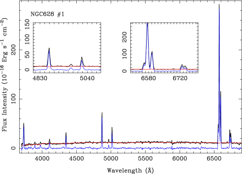
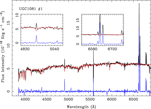
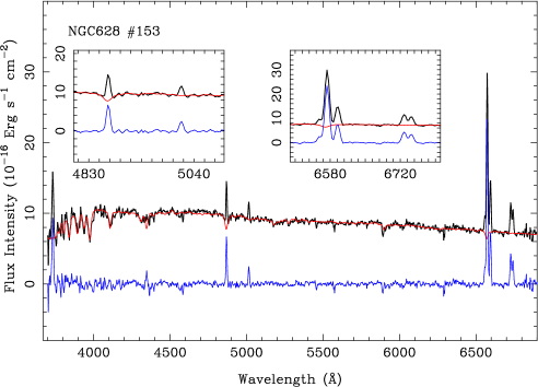
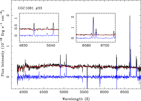
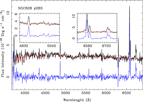
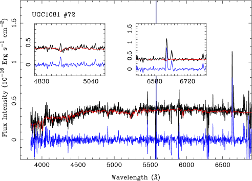
Figure 5: Spectra of three typical H ii regions for two different galaxies, NGC 628 (left panels), and UGC 1081 (right panels). The panels correspond, from top to bottom, to the brightest, average and faintest H ii regions with good quality data for each particular object. The spectral range shows all the emission lines analyzed in this article . From top to bottom: each panel shows the integrated spectra of the considered H ii region (solid-black), together with the best model for the underlying stellar population (solid-red), and the pure-gas spectra (solid-blue). The two boxes show a zoom of the same plots at the H$\beta$ and H$\alpha$ wavelength range.

Table 3 lists the results of this analysis, including, for each galaxy, its name, the number of derived spiral arms, a flag indicating the reliability of the results, and the parameters of the radial path for each arm, according to the described formula: $A$, $B$ and $C$. The quality flag is 1 for those galaxies with a clearly distinguised spiral structure and a well defined set of parameters to describe them, and for those galaxies without a well defined spiral structure (flocculent). Fig. 4 shows four examples of the derived spiral structure for the galaxies in our sample, including two cases with well defined spiral structure (NGC 628 and UGC 1081), one without a clear defined spiral structure (NGC 1637) and a clear flocculent case (UGC 9837).

We associated H ii regions to the nearest spiral arm by computing the minimum distance between the centroid of the H ii region and the radial distribution of the considered arm. The mean of these distances is then used as a scale-length to separate between H ii regions clearly associated with an arm, and possible inter-arm ones. A final flag is included in the corresponding catalogue table describing the coordinates of the detected H ii regions, indicating the nearest arm and the relative distance with respect to the median one. Table 4 illustrates the result of this analysis. It shows, for one single galaxy (UGC 9837), the absolute, relative, polar and deprojected coordinates of the 10 brightest H ii regions, together with identification of the nearest spiral arm, the Cartesian and angular distance to this arm and the spiralcentric distance (i.e. the distance to the center along the spiral arm). In this context brightness means the peak intensity within a certain H ii, as considered by HIIexplorer . In addition, we included in this table the systemic velocity and absolute luminosity of H$\alpha$ for each H ii, derived on basis of the emission line fitting described in Section 6.1.1. Similar parameters are derived for all the H ii regions in the different galaxies, as indicated in Appendix A. To our knowledge, this is the first attempt to perform an analytical association of H ii regions to a particular arm and/or to an inter-arm area in a survey mode.

Table 5: Emission line ratios with respect to H$\beta$, and H$\beta$ line intensity for the 10 brighest HII regions within UGC9837.

ID	F(H$\beta$)	$\frac{\mathrm{[OII]3727}}{\mathrm{H\beta}}$	$\frac{\mathrm{[OIII]5007}}{\mathrm{H\beta}}$	$\frac{\mathrm{[OI]6300}}{\mathrm{H\beta}}$	$\frac{\mathrm{H\alpha}}{\mathrm{H\beta}}$	$\frac{\mathrm{[NII]6583}}{\mathrm{H\beta}}$	$\frac{\mathrm{HeI6678}}{\mathrm{H\beta}}$	$\frac{\mathrm{[SII]6717}}{\mathrm{H\beta}}$	$\frac{\mathrm{[SII]6731}}{\mathrm{H\beta}}$
UGC9837-001	20.60$\pm$ 0.75	1.20$\pm$ 0.05	4.44$\pm$ 0.20	0.08$\pm$ 0.02	4.44$\pm$ 0.27	0.26$\pm$ 0.11	0.06$\pm$ 0.01	0.34$\pm$ 0.03	0.25$\pm$ 0.03
UGC9837-002	36.03$\pm$ 0.66	2.46$\pm$ 0.07	2.07$\pm$ 0.06	0.08$\pm$ 0.01	3.31$\pm$ 0.17	0.37$\pm$ 0.12	0.05$\pm$ 0.01	0.48$\pm$ 0.03	0.33$\pm$ 0.03
UGC9837-003	29.28$\pm$ 0.63	2.97$\pm$ 0.13	1.03$\pm$ 0.04	0.08$\pm$ 0.02	3.19$\pm$ 0.21	0.55$\pm$ 0.16	0.05$\pm$ 0.01	0.65$\pm$ 0.04	0.45$\pm$ 0.04
UGC9837-004	25.17$\pm$ 0.57	3.14$\pm$ 0.13	1.27$\pm$ 0.05	0.11$\pm$ 0.02	3.18$\pm$ 0.21	0.55$\pm$ 0.15	0.02$\pm$ 0.01	0.62$\pm$ 0.04	0.44$\pm$ 0.04
UGC9837-005	13.09$\pm$ 0.51	3.04$\pm$ 0.26	0.85$\pm$ 0.07	0.11$\pm$ 0.04	3.57$\pm$ 0.31	0.69$\pm$ 0.19	0.06$\pm$ 0.01	0.67$\pm$ 0.08	0.52$\pm$ 0.08
UGC9837-006	19.40$\pm$ 0.54	3.04$\pm$ 0.13	1.77$\pm$ 0.08	0.08$\pm$ 0.04	3.04$\pm$ 0.21	0.38$\pm$ 0.13	0.02$\pm$ 0.01	0.50$\pm$ 0.05	0.37$\pm$ 0.04
UGC9837-007	13.90$\pm$ 0.54	2.93$\pm$ 0.19	1.48$\pm$ 0.10	0.10$\pm$ 0.03	3.58$\pm$ 0.29	0.50$\pm$ 0.17	0.07$\pm$ 0.01	0.61$\pm$ 0.06	0.45$\pm$ 0.06
UGC9837-008	12.07$\pm$ 0.45	3.53$\pm$ 0.27	0.97$\pm$ 0.07	0.13$\pm$ 0.04	3.04$\pm$ 0.28	0.59$\pm$ 0.19	0.03$\pm$ 0.01	0.71$\pm$ 0.07	0.51$\pm$ 0.06
UGC9837-009	9.31$\pm$ 0.48	2.10$\pm$ 0.14	3.52$\pm$ 0.23	$\cdots$	3.35$\pm$ 0.27	0.27$\pm$ 0.11	0.04$\pm$ 0.01	0.38$\pm$ 0.06	0.29$\pm$ 0.06
UGC9837-010	13.46$\pm$ 0.51	3.52$\pm$ 0.23	1.35$\pm$ 0.09	0.18$\pm$ 0.05	3.30$\pm$ 0.29	0.52$\pm$ 0.19	0.04$\pm$ 0.01	0.73$\pm$ 0.07	0.52$\pm$ 0.06

Notes: H$\beta$ fluxes are in units of 10^-16 erg s^-1 cm^-2; All line intensities have been derived after subtracting the underlying stellar population, but without any further correction. The full catalogue of emission line ratios for the H ii regions analyzed in this object and the remaining ones discussed along this article are listed in Appendix A.

Table 6: Emission line equivalent with of the strongest emission lines analyzed, for the 10 brighest HII regions within UGC9837.

ID	Equivalent Width
	[OII]	H$\beta$	[OIII]	[OI]	H$\alpha$	[NII]	HeI	[SII]
	$\lambda 3727$		$\lambda 5007$	$\lambda 6300$		$\lambda 6583$	$\lambda 6678$	$\lambda 6717+6731$
UGC9837-001	-80.6$\pm$ 22.1	-83.8$\pm$ 17.6	-367.1$\pm$ 208.1	-8.0$\pm$ 1.2	-503.6$\pm$ 497.3	-29.6$\pm$ 33.4	-6.3$\pm$ 0.3	-69.5$\pm$ 7.1
UGC9837-002	-102.7$\pm$ 40.3	-53.9$\pm$ 6.4	-113.7$\pm$ 19.5	-6.0$\pm$ 0.5	-269.6$\pm$ 94.5	-30.2$\pm$ 13.4	-3.7$\pm$ 0.2	-69.2$\pm$ 5.5
UGC9837-003	-66.8$\pm$ 19.1	-22.7$\pm$ 2.1	-24.1$\pm$ 1.2	-2.2$\pm$ 0.2	-96.5$\pm$ 11.9	-16.5$\pm$ 3.2	-1.4$\pm$ 0.1	-34.0$\pm$ 1.3
UGC9837-004	-66.8$\pm$ 23.8	-23.2$\pm$ 2.2	-31.0$\pm$ 1.9	-3.2$\pm$ 0.3	-101.6$\pm$ 13.4	-17.9$\pm$ 3.6	-0.8$\pm$ 0.1	-34.6$\pm$ 1.4
UGC9837-005	-42.9$\pm$ 6.7	-14.0$\pm$ 1.4	-12.2$\pm$ 0.6	-1.9$\pm$ 0.3	-64.1$\pm$ 7.8	-12.3$\pm$ 2.3	-1.1$\pm$ 0.2	-22.1$\pm$ 0.8
UGC9837-006	-76.2$\pm$ 29.8	-30.0$\pm$ 2.5	-54.0$\pm$ 4.3	-3.1$\pm$ 0.7	-129.2$\pm$ 31.3	-16.3$\pm$ 5.5	-0.7$\pm$ 0.3	-38.1$\pm$ 1.8
UGC9837-007	-51.2$\pm$ 10.7	-21.1$\pm$ 2.4	-31.7$\pm$ 2.3	-2.6$\pm$ 0.4	-97.7$\pm$ 18.6	-13.5$\pm$ 3.7	-1.8$\pm$ 0.1	-30.2$\pm$ 1.3
UGC9837-008	-55.0$\pm$ 18.5	-15.2$\pm$ 1.7	-15.1$\pm$ 0.7	-2.4$\pm$ 0.3	-59.9$\pm$ 5.9	-11.8$\pm$ 2.0	-0.5$\pm$ 0.1	-25.1$\pm$ 0.8
UGC9837-009	-40.2$\pm$ 7.3	-22.9$\pm$ 2.9	-80.9$\pm$ 11.1	-2.6$\pm$ 1.4	-109.0$\pm$ 12.6	-8.5$\pm$ 1.9	-1.3$\pm$ 0.3	-21.5$\pm$ 1.2
UGC9837-010	-53.4$\pm$ 16.2	-16.5$\pm$ 1.7	-22.7$\pm$ 1.5	-4.0$\pm$ 0.5	-72.0$\pm$ 7.9	-11.4$\pm$ 2.3	-0.9$\pm$ 0.2	-28.1$\pm$ 1.4

Notes: All the listed equivalent widths are in units of Å. The full catalogue of equivalent widths for the H ii regions analyzed in this object and the remaining ones discussed along this article are listed in Appendix A.

6 Deriving the main spectroscopic properties of the H ii regions

6.1 Decoupling the emission lines from the underlying stellar population.

To extract the nebular physical information of each individual H ii region, the underlying continuum must be decoupled from the emission lines for each of the analyzed spectra. Several different tools have been developed to model the underlying stellar population, effectively decoupling it from the emission lines (e.g., Cappellari & Emsellem, 2004; Cid Fernandes et al., 2005; Ocvirk et al., 2006; Sarzi et al., 2006; Sánchez et al., 2007a; Koleva et al., 2009; MacArthur et al., 2009; Walcher et al., 2011; Sánchez et al., 2011). Most of these tools are based on the same principles, i.e., they assume that the stellar emission is the result of the combination of different (or a single) simple stellar populations (SSP), and/or the result of a particular star-formation history, whose emission is redshifted due to a certain systemic velocity, broadened and smoothed due a certain velocity dispersion and attenuated due to a certain dust content.

For the particular case of the H ii regions, the main purpose of this analysis is to provide a reliable subtraction of the underlying stellar population. For doing so, we performed a simple but robust modeling of the continuum emission. We use the routines described in Sánchez et al. (2011) and Rosales-Ortega et al. (2010), which provided us with certain parameters describing the physical components of the stellar populations (e.g., luminosity-weighted ages, metallicities and dust attenuation, together with the systemic velocity and velocity dispersion) and a set of parameters describing each of the analyzed emission lines (intensity, velocity and velocity dispersion). A simple SSP template grid was adopted, consisting of three ages (0.09, 1.00 and 17.78 Gyr) and two metallicities (0.0004 and 0.03). The models were extracted from the SSP template library provided by the MILES project (Vazdekis et al., 2010). The two considered metallicities are the most metal poor and most metal rich with the largest coverage range in ages, within the considered library. The oldest stellar population was selected to reproduce the reddest possible underlying stellar population, mostly due to larger metallicities than the one considered in our simplified model, although it is clearly older than the accepted cosmological time of the Universe. Our youngest stellar population is the 2nd youngest in the MILES library with both extreme metallicities. No appreciable difference was found between using this one or the youngest one ($\sim$80 Myr). Finally, we selected an average stellar population, of $\sim$1Gyr, required to reproduce the intermediate-to-blue stellar populations, and to produce more reliable corrections of the underlying stellar absorptions (Paper I). This library is clearly insufficient to describe in detail the nature of all the stellar populations and star formation histories. However, it covers the parameter space of possible stellar populations well enough to describe them at to 1st order, providing a clean residual information of the ionized gas. Evenmore, with a combination of the considered templates it is possible to reconstruct any of the SSP of the full MILES library within an accuracy similar to our photometric uncertainty ($\sim$10%, Paper I). Therefore, to include any other template is redundant for the main purpose of this analysis.

Fig. 5 illustrates the results of the fitting procedure for three H ii regions (the brightest, the average and the faintest one, in terms of H$\alpha$ luminosity) extracted from two typical galaxies (NGC 628 and UGC 1081). The figure shows for each H ii region the extracted spectrum (black line), together with the best multi-SSP model for the stellar population (red line), and the pure nebular emission spectrum (blue line).

6.1.1 Deriving the main properties of the emission lines

To derive the properties of the stronger emission lines detected in the stellar-population subtracted spectra, each line was fitted with a single Gaussian, coupled with the systemic velocity and velocity dispersion of different emission lines when needed (e.g., for doublets and triplets). This procedure provide us with the intensity, systemic velocity and velocity dispersion for each emission line. Note that by subtracting a stellar continuum model derived with a set of SSP templates, we are already taking into account (and correcting for, to a first order) the contribution of underlying absorption, which is particularly important in the H$\alpha$ and H$\beta$ lines.

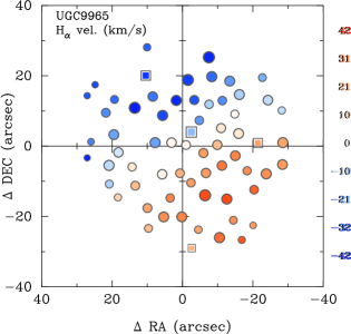
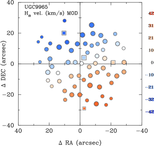
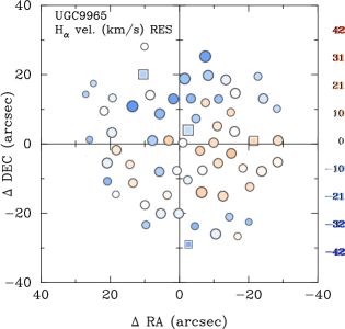
Figure 6: Left-panel: H$\alpha$ velocity field derived from the analysis of the H ii regions for UGC 9965. Central-panel: Best model fitted to the velocity map using a simple arctan velocity curve, and fitting the inclination, position angle and maximum rotational velocity. Right-panel: Residual of the subtraction of the model to the velocity map. Each plotted symbol in each panel represent an individual H ii region. The circles represent those H ii regions below the Kauffmann et al. (2003) demarcation line in the classical BPT diagram (Baldwin et al., 1981), and the squares corresponds to those ones located in the intermediate region between that line and the Kewley et al. (2001) one, as described later in the text. The size of the symbols are proportional to the H$\alpha$ intensity.

As discussed in Paper I, there are different issues that may affect the final quality of the individual spectra in the datacubes (uncleaned cosmic rays, trace problems, low transmission fibers, spectra near to the edge of the FoV and vignetting). These quality issues, that affect a reduced number of spaxels, propagate along the segregation, extraction and “stellar continuum” cleaning processes, and therefore they may affect the final quality of the “pure emission” spectra of the H ii regions. In order to minimize the impact of these issues on the final sample of H ii spectra, we have performed an automatic quality check. Only those “pure emission” spectra fulfilling the following criteria are flagged as good quality data:

1. The derived intensity for H$\alpha$ is above zero or below three times that of the brightest H ii region based on the narrow-band image intensity. The contrary may happen in case of problems with the fitting procedure, or problems with one or a few spectra of those that were co-added to derive the integrated spectrum (like a cosmic rays).

2. The fraction of spectral pixels with negative values in the original spectra, i.e. prior to the subtraction of the underlying stellar continuum, is lower than 10%. The contrary may happen in the outer regions of the galaxies, if there is any problem with the sky subtraction.

3. The fraction of spectral pixels in the “pure emission” spectra of the H ii region with a value below the median flux 1$\sigma$ within the wavelength range between 3900 and 6500Å, is at maximum three times lower than the median of this fraction for all the H ii regions in the same galaxy. This criterion is used to remove spectra strongly affected by the vignetting effect, which affects only $\sim$30%  of the data (Paper I).

4. The derived intensity for H$\alpha$ is more than five times above the background noise ($\sigma_{back}$), estimated as $\sigma_{back}=\sigma_{6300-6500}\leavevmode\nobreak\ FWHM_{line}$, where (i) $\sigma_{6300-6500}$ is the standard deviation of the continuum intensity once subtracted the underlying stellar component for the wavelength range between 6300 and 6500Å(i.e., a continuum adjacent to H$\alpha$); and (ii) $FWHM_{line}$ is the full width at half maximum derived for the emission line, as described before.

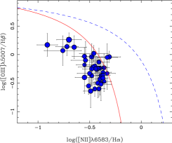
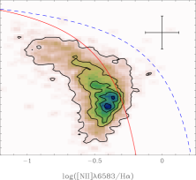
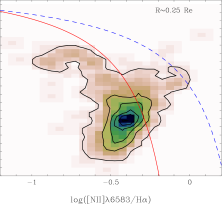
Figure 7: Left panel: [O iii] $\lambda$5007/H$\beta$ vs. [N ii] $\lambda$6583/H$\alpha$ diagnostic diagram for the average properties of the H ii regions galaxy by galaxy listed in Table 7. The error bars indicate the standard deviation from the mean value. Middle panel: Similar diagnostic diagram for all the emission line regions detected by the described analysis with good quality measurements of both parameters (2230 regions). The color image and contours show the density distribution of these regions. The first contour indicates the mean density, with each consecutive one increasing by four times this mean value. The Kauffmann et al. (2003) (red solid-line) and Kewley et al. (2001) (blue dashed-line) demarcation curves are usually invoked to distinguish between star-forming regions (below the red solid-line), and other source of ionization, like AGN/shocks/post-AGB (above the blue line). Regions between both lines are considered intermediate ones, indicating a mixed origin for the ionization. The error-bars at the top-left indicate the typical (mean) errors for the considered line ratios. Right panel: Similar diagram, including only the 124 regions at the core of each galaxy ($r<0.5r_{e}$, i.e., at $\sim 0.25r_{e}$ in average). The fraction of regions in the intermediate location is clearly higher.

The remaining regions are flagged out, masked, and the corresponding spectra are set to zero. The criteria were based on iterative experiments on the data, and visual inspections of hundreds of spectra, before and after subtracting the underlying continuum. Although the fraction of flagged-out/rejected spectra change from object to object, on average this final cleaning affects $\sim$15% of the H ii regions, as can be seen in Table 2. Finally, only those H ii regions with measured H$\beta$ emission line detected at $>$3$\sigma$ significance were considered for further analysis (e.g. Marino et al., 2012), although they were not masked out and their spectra were not set to zero. This criteria was included to consider only those regions with good line diagnostic ratios and well defined Balmer ratio, both required in further analysis. It further reduces the number of selected H ii regions by $\sim$5% on average, although is some cases the fraction is much larger (see Table 2). Due to the size of our original sample and the pseudo-random selection of H ii-regions that are affected by these issues, we consider that this last cleaning process will have little effect in the overall statistical significance of our survey.

Once derived the emission line intensities, we estimate their corresponding equivalent width for each H ii region and line. For doing so, instead of using the classical procedure (i.e., measuring the flux within a narrow-band wavelength range centred in the line and in two adjacent ones corresponding to the continuum), we make use of the results from our fitting analysis. We derive the equivalent width by dividing the emission line integrated intensities by the underlysing continuum flux density. We estimated the continuum as the median intensity in a band-width of 100$\AA$, centred in the line, using the gas-subtracted spectra provided by our fitting procedure. With this method we can estimate the equivalent width of nearby lines, which contaminate the measurements of this parameter using the classical method.

Table 5 illustrates the result of this analysis. It shows, for a sub-set of H ii regions in a particular galaxy (UGC 9837) the H$\beta$ line intensity and relative flux of some of the most prominent emission lines. Table 6 reports the equivalent widths for the corresponding emission lines and regions. The same parameters are derived for all the H ii regions in the different galaxies, as indicated in Appendix A.

6.1.2 Structural parameters of the galaxies

To understand the fundamental properties of the H ii regions and their relation with the overall evolution of galaxies, it is required to characterize the main structural parameters of these galaxies. We have collected the available information in public collections like NED (http://ned.ipac.caltech.edu/) and Hyperleda (http://leda.univ-lyon1.fr/). Table 1 already contains the most relevant parameters for the current study, including the morphological type, the redshift, the integrated $B$-band magnitude and the B-V color. All the galaxies in the sample are spirals by selection, but different kinds of spiral galaxies are covered, including galaxies with and without bars, galaxies showing rings, etc. The observed $B$-band magnitude is $\sim$14 mag, in average. However, the galaxies selected from the PINGS sample are in general brighter ($B\sim$11 mag). As expected, galaxies have blue colors ($B-V\sim$0.8 mag), although with a considerable dispersion. The covered absolute magnitudes range from $M_{V}\sim-$23 mag to $\sim-$18 mag. In summary, the sample covers typical members of the so-called blue cloud, from typical standard spiral galaxies to almost dwarfs.

The listed information was complemented with additional parameters, like the maximum rotation velocity, the inclination, the position angle and the effective radius (defined as the radius at which one half of the total light of the system is emitted), derived from the analysis of the data presented here. The first three parameters were derived from the modeling of the gas velocity pattern extracted from the the H$\alpha$ emission line fitting for the H ii regions, described in previous sections. The wide spatial coverage and high S/N of the H$\alpha$ emission line in the integrated spectra for each region guarantee a good determination of the velocity pattern. The rotation curve was fitted using a simple arctan model (Staveley-Smith et al., 1990),

$$v(r)=v_{sys}+\frac{2\leavevmode\nobreak\ v_{\rm rot}}{\pi}{\rm arctan}(s\cdot r-c)$$ (3)

where $v_{sys}$ is the systemic velocity of the gas and $v_{\rm rot}$ is the asymptotic rotation speed of the disc, $s$ characterizes the slope of $v(r)$ in the inner part of the galaxy, $r$ is the distance to the rotational center, and $c$ is the parameter that characterizes any offset in the rotation axis of the galaxy. A model of the velocity map was created by re-projecting the best fitting arctan function, taking into account the position angle and inclination of the galaxy. We fitted to the data following a similar procedure as the one described in Sánchez et al. (2012), using a $\chi^{2}$-minimization algorithm included in FIT3D (Sánchez et al., 2006b).

As an initial guess for the fitting, the position angle and inclination were derived from the isophotal analysis described later in this section, and the maximum rotational velocity was set to half of the maximum difference in velocity from receding to approaching velocities. For all the galaxies the rotational center is fixed to the location of the peak intensity in the $V$-band image created from the datacubes. The parameter $c$ is fixed to zero (i.e., it is assumed that there is no offset between the rotation and photometric centers). The $v_{sys}$ is fixed to the median value of the gas velocities for those H ii regions located in the inner regions ($r<$0.5$r_{max}$, where $r_{max}$ is the maximum distance to the center for all the H ii regions).

Finally $v_{\rm rot}$ and $s$ are fitted, together with the position angle and inclination of the galaxies, $v_{rot}$ is fitted within a range between $\sim$0.3 and 6 times the maximum velocity difference among the H ii regions, and $s$ is fitted between 0.1 and 10 arcsec^-1. Fig. 6 illustrates a typical result of this analysis, showing, for a particular galaxy (UGC 9837) the H$\alpha$ velocity map, the best fit model, and the residual. Despite the low inclination of the galaxies, in most of the cases it is possible to obtain a good model. In most of the cases the residual velocities ranges between $\pm$15 km s^-1, $\sim$15% of the maximum rotational velocity. This is expected due to random motions in the galaxies, compare e.g. Andersen et al. (2008); Neumayer et al. (2011).

The effective radius was derived based on an analysis of the azimuthal surface brightness (SB) profile, derived based on elliptical isophotal fitting of the ancillary $g$-band images collected for the galaxies (extracted from the SDSS imaging survey, York et al., 2000, and Paper I). When these ancillary images were not available we used the $B$-band (Paper I). In order to homogenize the dataset, both sets of SBs were transformed to the $B$-band using the average $g-B$ color for each galaxy. When both band images where available a comparison between the directly derived and the estimated surface brightness profile was performed, finding no significant differences in the average gradient. We note here that the observed $B$ and $g$-bands sample a range of wavelengths between $\sim$4150-4750Å and $\sim$4450-5210Å, respectively, due to the redshift range of the sample. Therefore, there is an inherent imprecision in the intrinsic wavelength range in this analysis.

The surface brightness profile was then fitted using a pure exponential profile, following the classical formula,

$$I=I_{0}\exp[-(r/r_{d})]$$ (4)

where $I_{0}$ is the central intensity, and $r_{d}$ is the disk scale-length (Freeman, 1970), using a simple polynomial regression fitting. Prior to this analysis, a visual inspection is performed to remove the inner-most values of the SB profile, strongly affected by seeing effect, and/or not following a linear relation due to the presence of other components like the bulge and/or bars.

The scale-length is used to derive the effective radius, defined as the radius at which the integrated flux is half of the total one, by integrating the previous formula, and deriving the relation:

$$r_{e}=1.67835r_{d}$$ (5)

The results of these analyses are included in Table 1. In average, the derived inclination agrees with the visual selection of the galaxies as face-on spirals. The average inclination is $\sim$33^∘, and only two galaxies have an inclination larger than 60^∘ (NGC 7570 and UGC 5100). This confirms our visual classification as face-on galaxies. The average maximum rotational velocity is $\sim$100 km s^-1, with a wide range of values, between $\sim$50 km s^-1 and $\sim$300 km s^-1 (values which are typical for spiral galaxies, e.g., Persic et al., 1996). Note that the effective radius ranges between $\sim$1.5 and $\sim$5.5 kpc.

7 Analysis and results

In this section we analyze both the mean statistical properties of the H ii regions and explore the possible regular patterns in their radial variations.

7.1 Statistical properties of the H ii regions

Despite the many different spectroscopic studies in extragalactic H ii regions, we still do not have the understanding of which are the statistical spectroscopic properties of these common star-forming regions. This is a fundamental problem that it is mostly due to the lack of big statistical samples, and the reduced number of coherent compilations. The lack of a well defined set of normal values for the most frequent parameters, like the diagnostic line ratios (e.g., [O iii]/H$\beta$ and/or [N ii]/H$\alpha$), ionization strength, dust attenuation and/or electron density is a clear limitation to understand if a particular set of H ii regions is different from the average, and if different at which significance level. To address this question a statistically significant, large sample of H ii regions is required, with well derived spectroscopic parameters, over a large sample of star-forming galaxies of different types. An additional requirement is good spatial coverage, not biased towards the outer (bright) H ii regions, which is a common bias in this kind of studies. Despite the large number of H ii regions catalogued in this work, the current sample is still incomplete to address this fundamental question. We will require a sample as the one that will be provided by a survey like CALIFA (Sánchez et al. 2012), without selection effects by galaxy types. However, the current catalogue of H ii regions is good enough to derive the statistical properties of these regions for a sub-set of galaxies: quiescent/non highly disturbed, field, average luminosity spiral galaxies.

Table 7: Median physical parameters of the ionized gas derived for the considered galaxies

Galaxy	LHα	EWHα	AV	$\frac{\mathrm{[OIII]}}{\mathrm{H\beta}}$	$\frac{\mathrm{[NII]}}{\mathrm{H\alpha}}$	U	$O/H$	rHII	ne
	(1)	(2)	(3)	(4)	(5)	(6)	(7)	(8)	(9)
2MASXJ1319+53	40.3 $\pm$ 0.6	-28.8 $\pm$ 6.7	1.4 $\pm$ 0.3	0.14 $\pm$ 0.16	-0.72 $\pm$ 0.11	-3.84 $\pm$ 0.34	8.48 $\pm$ 0.08	2.8 $\pm$ 6.1	$\cdots$
CGCG 071-096	40.0 $\pm$ 0.6	-35.0 $\pm$ 9.2	1.4 $\pm$ 0.5	-0.04 $\pm$ 0.23	-0.48 $\pm$ 0.10	-3.71 $\pm$ 0.21	8.59 $\pm$ 0.10	1.9 $\pm$ 1.8	$\cdots$
CGCG 148-006	40.0 $\pm$ 0.5	-24.0 $\pm$ 5.4	1.5 $\pm$ 0.6	-0.13 $\pm$ 0.24	-0.41 $\pm$ 0.09	$\cdots$	8.66 $\pm$ 0.10	$\cdots$	$\cdots$
CGCG 293-023	39.7 $\pm$ 0.5	-20.7 $\pm$ 4.5	1.5 $\pm$ 0.2	-0.20 $\pm$ 0.14	-0.45 $\pm$ 0.10	-4.06 $\pm$ 0.15	8.67 $\pm$ 0.05	1.6 $\pm$ 1.5	0.1 $\pm$ 2.6
CGCG 430-046	40.5 $\pm$ 0.5	-31.4 $\pm$ 7.6	1.5 $\pm$ 0.4	-0.26 $\pm$ 0.19	-0.43 $\pm$ 0.07	$\cdots$	8.70 $\pm$ 0.08	$\cdots$	$\cdots$
IC 2204	39.7 $\pm$ 0.6	-20.6 $\pm$ 4.9	1.6 $\pm$ 0.5	-0.23 $\pm$ 0.24	-0.36 $\pm$ 0.05	$\cdots$	8.75 $\pm$ 0.08	$\cdots$	2.0 $\pm$ 4.5
MRK 1477	41.0 $\pm$ 1.4	-39.1 $\pm$ 17.7	1.4 $\pm$ 0.4	-0.04 $\pm$ 0.10	-0.31 $\pm$ 0.11	-3.45 $\pm$ 0.31	8.64 $\pm$ 0.02	8.1 $\pm$ 3.5	$\cdots$
NGC 99	39.6 $\pm$ 0.6	-41.0 $\pm$ 12.3	1.2 $\pm$ 0.5	0.13 $\pm$ 0.20	-0.65 $\pm$ 0.12	$\cdots$	8.47 $\pm$ 0.10	$\cdots$	$\cdots$
NGC 3820	40.2 $\pm$ 0.3	-19.0 $\pm$ 3.2	0.9 $\pm$ 1.2	-0.60 $\pm$ 0.13	-0.45 $\pm$ 0.02	-3.78 $\pm$ 0.13	8.79 $\pm$ 0.04	3.5 $\pm$ 1.0	$\cdots$
NGC 4109	40.4 $\pm$ 0.7	-17.7 $\pm$ 3.0	1.9 $\pm$ 0.4	-0.37 $\pm$ 0.21	-0.39 $\pm$ 0.06	-3.93 $\pm$ 0.13	8.78 $\pm$ 0.09	3.8 $\pm$ 2.0	$\cdots$
NGC 7570	39.5 $\pm$ 0.7	-16.4 $\pm$ 3.6	1.4 $\pm$ 0.7	-0.24 $\pm$ 0.16	-0.40 $\pm$ 0.04	$\cdots$	8.71 $\pm$ 0.04	$\cdots$	1.6 $\pm$ 9.4
UGC 74	39.2 $\pm$ 0.5	-12.5 $\pm$ 3.5	1.3 $\pm$ 0.5	-0.47 $\pm$ 0.18	-0.36 $\pm$ 0.07	$\cdots$	8.77 $\pm$ 0.05	$\cdots$	2.7 $\pm$ 3.8
UGC 233	40.0 $\pm$ 0.8	-34.0 $\pm$ 10.4	1.3 $\pm$ 0.5	0.02 $\pm$ 0.14	-0.46 $\pm$ 0.14	$\cdots$	8.58 $\pm$ 0.08	$\cdots$	$\cdots$
UGC 463	39.7 $\pm$ 0.5	-23.6 $\pm$ 4.9	1.6 $\pm$ 0.4	-0.60 $\pm$ 0.14	-0.41 $\pm$ 0.06	$\cdots$	8.79 $\pm$ 0.04	$\cdots$	0.4 $\pm$ 3.6
UGC 1081	38.7 $\pm$ 0.4	-12.9 $\pm$ 3.6	1.1 $\pm$ 0.4	-0.31 $\pm$ 0.17	-0.37 $\pm$ 0.08	$\cdots$	8.73 $\pm$ 0.07	$\cdots$	0.4 $\pm$ 1.5
UGC 1087	39.1 $\pm$ 0.3	-21.9 $\pm$ 5.8	1.0 $\pm$ 0.5	-0.24 $\pm$ 0.18	-0.42 $\pm$ 0.08	$\cdots$	8.67 $\pm$ 0.08	$\cdots$	3.0 $\pm$ 4.7
UGC 1529	40.0 $\pm$ 0.5	-12.6 $\pm$ 2.6	1.7 $\pm$ 0.5	-0.49 $\pm$ 0.22	-0.40 $\pm$ 0.06	$\cdots$	8.77 $\pm$ 0.08	$\cdots$	11.2 $\pm$ 20.4
UGC 1635	38.8 $\pm$ 0.4	-11.2 $\pm$ 2.2	1.4 $\pm$ 0.6	-0.36 $\pm$ 0.16	-0.37 $\pm$ 0.07	$\cdots$	8.73 $\pm$ 0.06	$\cdots$	2.3 $\pm$ 3.5
UGC 1862	38.1 $\pm$ 0.4	-10.6 $\pm$ 3.0	1.5 $\pm$ 0.5	-0.18 $\pm$ 0.19	-0.55 $\pm$ 0.08	$\cdots$	8.61 $\pm$ 0.06	$\cdots$	1.4 $\pm$ 1.8
UGC 3091	39.3 $\pm$ 0.5	-25.4 $\pm$ 7.6	1.3 $\pm$ 0.4	-0.22 $\pm$ 0.28	-0.47 $\pm$ 0.14	$\cdots$	8.67 $\pm$ 0.14	$\cdots$	1.1 $\pm$ 2.4
UGC 3140	39.8 $\pm$ 0.5	-23.2 $\pm$ 5.2	1.6 $\pm$ 0.4	-0.43 $\pm$ 0.22	-0.40 $\pm$ 0.06	$\cdots$	8.76 $\pm$ 0.05	$\cdots$	1.8 $\pm$ 4.3
UGC 3701	39.3 $\pm$ 0.3	-26.3 $\pm$ 8.6	1.6 $\pm$ 0.5	-0.03 $\pm$ 0.15	-0.55 $\pm$ 0.12	$\cdots$	8.57 $\pm$ 0.07	$\cdots$	1.7 $\pm$ 2.0
UGC 4036	39.8 $\pm$ 0.5	-12.3 $\pm$ 3.7	1.5 $\pm$ 0.5	-0.33 $\pm$ 0.28	-0.33 $\pm$ 0.08	$\cdots$	8.78 $\pm$ 0.06	$\cdots$	2.7 $\pm$ 3.3
UGC 4107	39.7 $\pm$ 0.5	-19.5 $\pm$ 3.5	1.5 $\pm$ 0.5	-0.25 $\pm$ 0.20	-0.44 $\pm$ 0.04	$\cdots$	8.69 $\pm$ 0.06	$\cdots$	2.8 $\pm$ 2.1
UGC 5100	39.9 $\pm$ 0.7	-19.5 $\pm$ 4.6	1.2 $\pm$ 0.4	-0.05 $\pm$ 0.24	-0.33 $\pm$ 0.10	-3.58 $\pm$ 0.39	8.72 $\pm$ 0.10	2.9 $\pm$ 2.5	$\cdots$
UGC 6410	39.7 $\pm$ 0.5	-25.4 $\pm$ 5.7	1.3 $\pm$ 0.5	-0.25 $\pm$ 0.21	-0.48 $\pm$ 0.09	-3.68 $\pm$ 0.27	8.65 $\pm$ 0.09	1.2 $\pm$ 0.7	$\cdots$
UGC 9837	38.7 $\pm$ 0.5	-29.5 $\pm$ 12.0	0.7 $\pm$ 0.4	0.07 $\pm$ 0.26	-0.76 $\pm$ 0.18	-3.53 $\pm$ 0.45	8.48 $\pm$ 0.14	0.4 $\pm$ 0.2	0.5 $\pm$ 2.7
UGC 9965	39.7 $\pm$ 0.3	-27.3 $\pm$ 8.9	1.7 $\pm$ 0.5	-0.10 $\pm$ 0.33	-0.54 $\pm$ 0.14	-3.76 $\pm$ 0.29	8.62 $\pm$ 0.14	1.4 $\pm$ 0.7	4.5 $\pm$ 12.1
UGC 11318	40.1 $\pm$ 0.5	-34.3 $\pm$ 7.9	1.8 $\pm$ 0.4	-0.50 $\pm$ 0.26	-0.42 $\pm$ 0.08	-3.68 $\pm$ 0.24	8.76 $\pm$ 0.07	2.0 $\pm$ 1.1	$\cdots$
UGC 12250	39.6 $\pm$ 0.5	-21.0 $\pm$ 3.7	1.2 $\pm$ 0.5	-0.41 $\pm$ 0.10	-0.37 $\pm$ 0.05	$\cdots$	8.75 $\pm$ 0.03	$\cdots$	$\cdots$
UGC 12391	39.7 $\pm$ 0.3	-21.5 $\pm$ 4.7	1.4 $\pm$ 0.4	-0.37 $\pm$ 0.18	-0.48 $\pm$ 0.06	$\cdots$	8.70 $\pm$ 0.07	$\cdots$	3.9 $\pm$ 21.8
NGC 628	38.7 $\pm$ 0.5	-50.4 $\pm$ 26.7	1.1 $\pm$ 0.5	-0.40 $\pm$ 0.28	-0.55 $\pm$ 0.09	-3.75 $\pm$ 0.29	8.68 $\pm$ 0.10	0.5 $\pm$ 0.5	0.5 $\pm$ 3.1
NGC 1058	38.7 $\pm$ 0.5	-24.8 $\pm$ 11.7	1.0 $\pm$ 0.4	-0.33 $\pm$ 0.33	-0.50 $\pm$ 0.12	-3.82 $\pm$ 0.27	8.70 $\pm$ 0.12	0.5 $\pm$ 0.3	0.4 $\pm$ 2.3
NGC 1637	38.8 $\pm$ 0.5	-19.0 $\pm$ 6.7	1.3 $\pm$ 0.4	-0.52 $\pm$ 0.29	-0.39 $\pm$ 0.10	-3.84 $\pm$ 0.25	8.79 $\pm$ 0.08	0.5 $\pm$ 0.8	1.5 $\pm$ 2.6
NGC 3184	39.2 $\pm$ 0.4	-43.0 $\pm$ 15.7	1.3 $\pm$ 0.5	-0.64 $\pm$ 0.29	-0.49 $\pm$ 0.07	-3.79 $\pm$ 0.27	8.80 $\pm$ 0.08	1.0 $\pm$ 0.6	0.7 $\pm$ 2.7
NGC 3310	39.8 $\pm$ 0.8	-133.0 $\pm$ 51.8	0.2 $\pm$ 0.2	0.26 $\pm$ 0.12	-0.70 $\pm$ 0.12	-3.31 $\pm$ 0.44	8.42 $\pm$ 0.07	1.0 $\pm$ 1.4	0.5 $\pm$ 1.8
NGC 4625	39.3 $\pm$ 0.4	-24.6 $\pm$ 6.0	0.6 $\pm$ 0.4	-0.55 $\pm$ 0.15	-0.51 $\pm$ 0.04	-3.81 $\pm$ 0.16	8.75 $\pm$ 0.05	1.0 $\pm$ 0.3	0.3 $\pm$ 1.8
NGC 5474	38.4 $\pm$ 0.4	-64.6 $\pm$ 28.0	0.7 $\pm$ 0.4	0.17 $\pm$ 0.20	-0.91 $\pm$ 0.10	-3.49 $\pm$ 0.44	8.39 $\pm$ 0.08	0.3 $\pm$ 0.2	0.2 $\pm$ 3.0
Mean	39.5 $\pm$ 0.6	-28.4 $\pm$ 20.8	1.3 $\pm$ 0.4	-0.25 $\pm$ 0.23	-0.47 $\pm$ 0.13	-3.71 $\pm$ 0.18	8.67 $\pm$ 0.10	1.9 $\pm$ 1.8	1.9 $\pm$ 2.3

Notes: The table shows the median values and standard deviations of the following physical parameters: (1) Decimal logarithm of the dust corrected luminosity of H$\alpha$ in erg s^-1; (2) Equivalent width of the pure H$\alpha$ emission line expressed in Å(values decontaminated from the underlying stellar absorption); (3) Dust attenuation derived from the H$\alpha$/H$\beta$ line ratio; (4) [OIII]$\lambda$5007/H$\beta$ line ratio, in decimal logarithm scale; (5) [NII]$\lambda$6583/H$\alpha$ line ratio, in decimal logarithm scale; (6) Ionization parameter; (7) Oxygen abundance, 12 + log(O/H), derived using the O3N2 indicator; (8) Stömgren radius calculated for the HII regions in units of 100 parsecs; (9) Electron density in units of 100 electrons per cm³.

Among the several different spectroscopic parameters describing H ii regions, we have analyzed a set of them based on the strongest detected emission lines: (i) EW_Hα, the equivalent width of the H$\alpha$ emission line. This parameter is directly related to the fraction of very young stars ($\sim$ 10 Myr), and can be used to estimate the aging process of the ionizing population; (ii) A_V, the dust attenuation derived from the H$\alpha$/H$\beta$ Balmer decrement. To derive it the extinction law by Cardelli et al. (1989) was assumed, with $R_{\rm V}=$3.1, and the theoretical value for the unobscured line ratio for case B recombination of H$\alpha$/H$\beta=2.86$, for $T_{e}$=10,000 K and $n_{e}$=100 cm^-3 (Osterbrock, 1989); (iii) two typical diagnostic line ratios, [O iii] $\lambda$5007/H$\beta$ and [N ii] $\lambda$6583/H$\alpha$, that define the nature of the ionization source; (iv) the ionization parameter, estimated as ${\rm log}_{10}U=-3.02-0.80{\rm log}_{10}([@series{\mathbf{O\,\mathsc{ii}}}]/[@series{\mathbf{O\,\mathsc{iii}}}])$, a measurement of the strength of the ionization radiation (Díaz et al., 2000); (v) the oxygen abundance, 12 + log(O/H), derived using the O3N2 indicator defined by Pettini & Pagel (2004), that estimates the gas enrichment; (vi) r_HII, the Strömgren radius of the H ii regions (Osterbrock, 1989), i.e., a hint of the size of the H ii regions based on pressure equilibrium considerations, and (vii) $n_{e}$, the electron density derived from the [S ii] doublet line ratio, i.e., a proxy to the density of the ionized gas (e.g., Osterbrock, 1989).

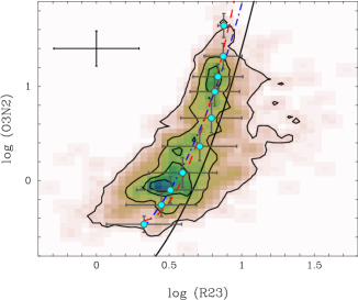
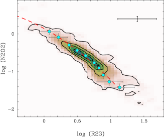
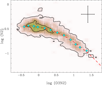
Figure 8: Left-panel: Distribution of the O3N2 vs. R₂₃ line ratios for all the 1142 H ii regions with detected [O ii] $\lambda$3727 emission line. The image and contours show the density distribution of both parameters. The first contours is at the mean density, with a regular spacing of four times this value for each consecutive contour. The red-dashed line shows the best fit found using a 2nd-order polynomial function between the two considered parameters. The light-blue solid-circles indicate the median values of both parameters, with their corresponding standard deviations represented as error bars, for consecutive bins of 0.10 in $\Delta$O3N2. The black solid line shows the relation expected between both parameters when they are used to derive the same oxygen abundance, assuming the Tremonti et al. (2004) fit for R₂₃ and the Pettini & Pagel (2004) calibration for O3N2. The dot-dashed blue line shows the same relation, if the oxygen abundance derived based on R₂₃ was 70% of the one derived using the Tremonti et al. (2004) fit. Central panel: Similar plot for the distributions of the N2O2 line ratio vs. R₂₃, for the same H ii regions. In this case the light-blue solid-circles indicate the median values and corresponding standard deviations of the parameters for consecutive bins of 0.10 in $\Delta$N2O2. Right panel: Similar plot for the distribution of the N2 line ratio vs. O3N2. The blue solid circles indicate the median values of both parameters, with their corresponding standard deviations, for consecutive bins of 0.10 in $\Delta$O3N2. The red dashed-line shows the best fit found using a 2nd-order polynomial function between both parameters. In the three panels the typical/median errors of the represented parameters are represented as a black error-bar.

Table 7 shows the mean values and standard deviations of the considered parameters for the H ii regions of each galaxy, together with the mean value for all the galaxies. Based on this analysis, it is possible to describe two kind of behaviors: on one hand, some of the parameters have a large variation object by object (e.g., EW[H_α], r_HII), reflecting the different physical conditions of H ii regions in individual galaxies. On the other hand, there are parameters with a well defined mean value and little variation object-by-object, and even region by region (e.g., the dust attenuation, the ionization parameter and the oxygen abundance). i.e., despite of the many differences between the considered galaxies (luminosity, morphology, color), and the physical conditions in each H ii region, it is possible to define a statistically meaningful standard mean value for certain spectroscopic parameters.

Due to the particular sample of galaxies studied here, and the large number of H ii regions explored, we consider that these values define the average physical conditions of H ii regions for spiral galaxies in the Local Universe. They can either be used to determine whether a particular (spiral) galaxy deviates from the average population (i.e., it is metal rich or poor and/or it is more or less dusty), or as the anchor point of chemical evolution of ionized gas along cosmological times. The H ii regions discussed here have a range of H$\alpha$ luminosities between 10³⁷ and 10⁴¹ erg s^-1, with a well defined bell-like shape centred at 10^39.5±0.6 erg s^-1. Therefore, most of our regions correspond to intermediate/luminous ones, as indicated in Section 2. These H ii regions are expected to have a typical size of few to several hundreds of parsecs, at the edge of our spatial resolution or below.

For some parameters the mean value is well defined (i.e., it shows a dispersion around the mean value of the order of the estimated error). Thus it is a good characterization of the considered property of the ionized gas. However, it is important to remember that the variations within the considered distributions reflect changes in the physical conditions of the ionized nebulae, either within each galaxy, or galaxy by galaxy. To illustrate this effect we present in Fig. 7 three panels showing the classical [O iii]/H$\beta$ vs. [N ii]/H$\alpha$ BPT (Baldwin et al., 1981) diagnostic diagram for (i) the average values shown in Table 7; (ii) all the emission line regions detected using the procedure described in previous sections; and (iii) those emission line regions located at the center of the galaxies ($r<0.5r_{e}$). In each panel, we include the Kauffmann et al. (2003) and Kewley et al. (2001) demarcation curves. These curves are usually invoked to distinguish between star-forming regions, and other sources of ionization, like AGN/Shocks/post-AGBs. The location within both curves is normally assigned to a mix origin for the ionization and/or contamination by different sources of ionization. Since our sample is dominated by H ii regions, most of the regions lie in the demarcation region corresponding to star-forming areas, although a few of them are located in the so-called intermediate region. There are clear differences galaxy by galaxy, reflecting changes in the average oxygen abundance and ionization strength. On the other hand, it is clear that for the regions located in the center of the galaxies the fraction of emission line regions lying in the intermediate region is larger. This is expected since these are the regions more likely to be contaminated by other ionization sources than star-formation: e.g., central low-intensity AGNs, Shocks, post-AGB stars. It is beyond the scope of this article to determine the real nature of this ionization in the central regions. This will require a more detail analysis and the use of other more suitable diagnostic diagrams like [NII]/H$\alpha$ vs. [SII]/H$\alpha$ and/or [NII]/H$\alpha$ vs. [SII]6717,6731/$H\alpha$, to distinguish between HII regions, SNR and PNe. We just want to emphasize that if there is any possible contamination, this will more likely affect only the central regions. This clearly indicates a change in the ionization conditions galaxy by galaxy and across the optical extension of each galaxy. One may wonder whether the described differences are induced by the errors in the represented parameters. However, most probably this is not the case. The typical error is represented as an error-bar in the central panel of the figure, showing that it is smaller than the dispersion of values found (in particular for the range of [N ii]/H$\alpha$ values sampled).

Another possible explanation is that the large range of redshifts/distance has an effect in variation of some properties due to our coarse resolution. This could be the case for the differences found for the Stömgren radius or the luminosity of H$\alpha$ for some galaxies, like NGC 628, at a distance of $\sim$9 Mpc and Mrk 1477, at a distance of $\sim$90 Mpc. However, this cannot be the only explanation, since there are other galaxies with large difference in both parameters at lower relative cosmological distance, like UGC 6410 (at $\sim$80 Mpc), and NGC 4109 (at $\sim$100 Mpc).

In summary, although the mean values listed in Table 7 are somehow representative of the average ionization conditions in each galaxy, they do not show the complete picture, since there are clear/expected variations of the ionizing condition across the optical extension of the galaxies.

7.1.1 Strong-line calibrators of the oxygen abundance

One of the fundamental parameters that can be derived from the spectroscopic analysis of H ii regions is the oxygen abundance. Oxygen is one of the easiest elements to measure in H ii regions, due to the strength of its emission lines in the optical wavelength range. This is fortunate, since O is an $\alpha$-process element made directly in short-lived massive stars (dominant in H ii regions). It is a good proxy of all heavy elements, comprising $\sim$50% of all the metals by mass in all the Universe. Therefore, it is a fundamental parameter to understand the evolution of the stellar populations galaxy-by-galaxy and at different locations within the same galaxy.

Accurate abundance measurements for the ionized gas in galaxies require the determination of the electron temperature (T_e) in this gas which is usually obtained from the ratio of auroral to nebular line intensities, such as [O iii] $\lambda$4363/[O iii] $\lambda\lambda$4959,5007 (Osterbrock, 1989). It is well known that this procedure is difficult to carry out for metal-rich galaxies since, as the metallicity increases, the electron temperature decreases (as the cooling is via metal lines) and the auroral lines eventually become too faint to measure. Therefore, calibrators based on strong emission lines are used. Lopez-Sanchez et al. (2012) has recently presented a revision on the different methods, showing their main problems, and illustrating in which range/conditions then can be applied. In particular they describe the most widely used methods in large galaxy surveys, that rely on the measurement of different strong emission lines (and line ratios) in the H ii region spectrum and empirical calibrations with regions of well-known oxygen abundance.

One of the first strong emission line methods was proposed by Pagel et al. (1979). It relies upon the ratio of [O ii] $\lambda$3727 and [O iii] $\lambda\lambda$4959,5007 with respect to H$\beta$, the so-called R₂₃ ratio:

$${\rm R_{23}}=\frac{I([@series{\mathbf{O\,\mathsc{ii}}}]\leavevmode\nobreak\ \lambda 3727)+I([@series{\mathbf{O\,\mathsc{iii}}}]\leavevmode\nobreak\ \lambda\lambda 4959,5007)}{I({\rm H}\beta)}$$ (6)

However, this index is double valued, with two different calibrations for low metallicity (12 + log(O/H)$<$8.1) and high metallicity (12 + log(O/H)$>$8.4) H ii regions. There is an ill-defined regime where regions with the same R₂₃ ($>0.7$) value have oxygen abundances that differ by almost and order of magnitude (e.g., see Figure A1 in López-Sánchez & Esteban, 2010). Ratios such as O3N2 (Alloin et al., 1979; Pettini & Pagel, 2004), N2O2 (van Zee et al., 1998; Dopita et al., 2000), N2 (van Zee et al., 1998; Pettini & Pagel, 2004; Denicoló et al., 2002), and many others, were introduced in an attempt to solve this ambiguity in the derived abundances:

$${\rm O3N2} = \frac{I([@series{\mathbf{O\,\mathsc{iii}}}]\leavevmode\nobreak\ \lambda 5007)/I({\rm H}\beta)}{I([@series{\mathbf{N\,\mathsc{ii}}}]\leavevmode\nobreak\ \lambda 6584)/I({\rm H}\alpha)}$$ (7)

$${\rm N2O2} = \frac{I([@series{\mathbf{N\,\mathsc{ii}}}]\leavevmode\nobreak\ \lambda 6584)}{I([@series{\mathbf{O\,\mathsc{ii}}}]\leavevmode\nobreak\ \lambda 3727)}$$ (8)

$${\rm N2} = \frac{I([@series{\mathbf{N\,\mathsc{ii}}}]\leavevmode\nobreak\ \lambda 6584)}{I(H\alpha)}$$ (9)

Some of these indicators are strongly affected by the dust attenuation, like N2O2 and ${\rm R_{23}}$, and should be determined after correcting it. Others are less sensitive to dust attenuation. Furthermore, empirical calibrations based on direct estimates of the electron temperature of the ionized gas systematically provide oxygen abundances which are systematically 0.2-0.4 dex lower than those derived using calibrations based on photoionization models (e.g. Lopez-Sanchez et al., 2012).

To derive the main statistical properties of the oxygen abundance, we adopted the O3N2 ratio. This ratio is less dependent on the adopted correction for the dust attenuation, and uses emission lines covered by our wavelength range for all the galaxies in the current sample. Like the N2O2 indicator, it relies on the use of the intensity of [N ii]. In the high metallicity regime –12+log(O/H)$\gtrsim$8.3– nitrogen is produced by both massive and intermediate-mass stars (e.g. Pilyugin et al., 2003) and hence nitrogen is essentially a secondary element in this metallicity regime. The [N ii]/H$\alpha$ ratio will therefore become stronger with on-going star formation and evolution of galaxies, until very high metallicities are reached, i.e. 12 + log(O/H)$>$9.0, where [N ii] starts to become weaker due to the very low electron temperature caused from strong cooling by metal ions. However, N2 is an indirect estimator that may depend on the ionization strength.

We should remember here that for $\sim$50% of our targets [O ii] $\lambda$3727 was not covered by the observed wavelength range, and therefore, the fraction of H ii regions with R₂₃ and N2O2 line ratios is just half of the total number of regions, since both rely on this emission line. The direct estimate based on the electron temperature is of less use. The fraction of H ii regions with reliable measurements of the the auroral [O iii] $\lambda$4363 is just $\sim$10%. This line is either too faint or is blended and/or strongly affected by the Hg I 4348 atmospheric light pollution emission line, and even H$\gamma$, in most of the cases. Due to that we consider O3N2 the best estimator for the purpose of the current study. In general it is considered that this estimator is valid for the range between $-$1$<\log{\rm O3N2}<$1.9 (e.g. Yin et al., 2007). However it becomes less reliable for metallicities lower than 12 + log(O/H)$<$8.3 (e.g. Yin et al., 2007; Lopez-Sanchez et al., 2012).

It is beyond the scope of the current study to make a detailed comparison of the oxygen abundances derived using the different proposed methods, in a similar way as it was presented by Kewley & Ellison (2008); Lopez-Sanchez et al. (2012). However, it is a good sanity check to compare between some of the most frequently used ones. This comparison will help us to understand (1) if the H ii regions described here are in the valid range for the adopted metallicity indicator; (2) which are the real differences in using one indicator or another; and (3) how accurate is the adopted correction for the dust attenuation, since we can compare indicators with different degree of dependency on the adopted correction.

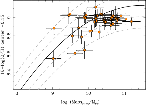
Figure 9: Relation between the stellar mass, in units of the solar masses, and the oxygen abundance at the central regions ($r<0.2\leavevmode\nobreak\ r_{e}$), using the O3N2 calibration, for the galaxies considered in the current study (solid circles). The black-solid line shows the relation found by Tremonti et al. (2004) for the star-forming galaxies in the SDSS sample, corrected for the mismatch between their suggested calibrator and the currently used here (i.e., $-$0.15 dex). The grey-dashed lines show the $\sim$1$\sigma$ and $\sim$2$\sigma$ range around this relation.

Fig. 8, shows the comparison between O3N2, N2O2 and N2 indicators, all of them using the [N ii] $\lambda$6584 line, with respect to the solely oxygen-based R₂₃ ratio. Only the H ii regions with detected [O ii] $\lambda$3727 emission line have been included in this plot (1142 individual regions). In each panel it is shown the image and contours of the density distribution of both parameters. The red-dashed lines show the best fits found using a 2nd-order polynomial function between the two considered parameters. The light-blue solid-circles indicate the median values of both parameters, with their corresponding standard deviations represented as error bars, for consecutive equally spaced bins of 0.10 dex of the parameters shown. In all cases the distributions are similar to the ones previously described in the literature between the considered estimators and/or their derived abundance (e.g. van Zee et al., 1998; Yin et al., 2007; Rosales-Ortega et al., 2011). However, in none of the precedent studies the distributions are shown with such a large statistical sample.

In the three cases there is a clear correlation between the median/high dense distribution of both parameters. The correlation is stronger for N2O2 vs. R₂₃ and for N2 vs. O3N2 than for the remaining one. The first of this relations is well described by a 2rd order polynomial function:

$$\log{\rm N2O2} = 0.15-0.97\log{\rm R_{23}}-0.39[\log{\rm R_{23}}]^{2}$$ (10)

The dispersions of each parameter around the best fit curve are $\sigma_{\rm N2O2}\sim$0.11 and $\sigma_{\rm R23}\sim$0.17, respectively. The dispersion in the y-axis is very similar to the typical (mean) errors of the corresponding line ratio, $e_{\rm N2O2}\sim 0.07$. This indicate that most of the dispersion is due to the errors in the derived line ratios, and not in a physical dependence with a third parameter.

The second relation is also well described by a 2rd order polynomical function:

$$\log{\rm N2} = 0.46-0.12\log{\rm O3N2}-0.19[\log{\rm O3N2}]^{2}$$ (11)

For this distribution, the dispersions of each parameter around the best fit curve are $\sigma_{N2}\sim$0.10 and $\sigma_{\rm O3N2}\sim$0.32, respectively. Once more, the dispersion in the y-axis is very similar to the typical (mean) errors of the corresponding line ratio, $e_{\rm N2}\sim 0.17$. Again, this indicates that most of the dispersion is due to the errors in the measured line ratios, rather than a unknown relation with a third parameter.

Finally, the correlation is less tight for the the O3N2 and R₂₃ parameters, with a broader dispersion and a tail for R${}_{23}>0.7$. In this case a 2nd order polynomial function describe will enough

$$\log{\rm O3N2}=0.18-3.76\log{\rm R_{23}}+5.88[\log{\rm R_{23}}]^{2}$$ (12)

However, the dispersion around the best curve is larger for the O3N2 parameter, $\sigma_{\rm O3N2}\sim$0.62, but similar for the R₂₃ one, $\sigma_{\rm R23}\sim$0.17. This dispersion cannot be explained only by the larger typical (mean) error of the represented line ratios ($e_{\rm O3N2}\sim 0.2$ and $e_{\rm R23}\sim 0.3$, respectively), and most probably indicates a real difference and/or a dependence with a third parameter (like the ionization strength).

Tremonti et al. (2004) proposed a non linear fit of the oxygen abundance for the R₂₃ indicator that is nowadays widely used. Assuming that this calibration derives a similar oxygen abundance than the one proposed by Pettini & Pagel (2004) is is possible to derive the following relation between both parameters:

$$y=-1.406+0.987x+0.825x^{2}+1.396x^{3}$$ (13)

where: $y=\log{\rm O3N2}$ and $x=\log{\rm R_{23}}$. This relation has a similar shape than the one described before for the range of values corresponding to 0.5$<$ R${}_{23}<$1, however it is offset by $\sim$0.15 dex in R₂₃ and $\sim-$0.5 dex in O3N2. The oxygen abundance derived using both indicators agrees if it is assumed that the Tremonti et al. (2004) relation overestimate the abundance by $\sim$30%. The difference is due to the photoionization models adopted by Tremonti et al. (2004), as discussed in Lopez-Sanchez et al. (2012). Correcting for that difference, the derived relation between O3N2 and R₂₃ agrees with the one found with our dataset (blue dashed-dotted line in Fig. 8). Therefore, the oxygen abundance derived using the Pettini & Pagel (2004) and Tremonti et al. (2004) calibrators do not provide consistent results, as already pointed out in previous studies (e.g. Lopez-Sanchez et al., 2012). However, the discrepancy is in the zero-point of the adopted calibration, rather than in the actual values for the indicators. The dispersion is tighter for R${}_{23}<0.7$, i.e., the parameter range for which the oxygen abundance is not double valued. For values of R₂₃ larger than 0.7 we found that the discrepancy with the derived relation shows a trend with the ionization parameter, being larger at lower values of $U$.

Kewley & Ellison (2008) performed a comparison between the oxygen abundance derived using different strong line indicators, based on analysis of large sample of SDSS spectra of star-forming galaxies. They derived a set of transformation for the different analyzed indicators, including R₂₃ and O3N2. These transformation are consistent with the ones presented here, for the range of abundance for which their are valid (see Table 3 in Kewley & Ellison, 2008).

Table 8: Results of the analysis of the radial gradients of a set of properties.

Parameter	Ngal	rcor	$\sigma_{r}$	meda	$\sigma_{\rm a}$	erra	medb	$\sigma_{\rm b}$	errb
(1)	(2)	(3)	(4)	(5)	(6)	(7)	(8)	(9)	(10)
$\mu_{\rm B}$	25	0.98	0.02	21.64	0.84	0.26	1.68	0.01	0.23
$B-V$	25	0.50	0.22	0.87	0.20	0.30	-0.20	0.15	0.27
rHII (100 pc)	11	0.61	0.24	2.57	0.25	0.30	-0.48	0.20	0.26
12 + log10(OH)	25	0.60	0.25	8.84	0.13	0.30	-0.12	0.11	0.27
log10($|$EWHα$|$)	25	0.57	0.21	0.95	0.32	0.25	0.51	0.28	0.22
log10($[$NII$]$/H$\alpha$)	25	0.54	0.24	-0.41	0.13	0.30	-0.10	0.13	0.27
log10($[$OIII$]$/H$\beta$	25	0.53	0.28	-0.59	0.32	0.25	0.29	0.26	0.22
log$(U)$	11	0.35	0.24	-3.93	0.29	0.04	0.09	0.12	0.08
ne (100 cm-3)	22	0.21	0.13	2.48	7.79	0.26	0.31	0.67	0.24
AV (mag)	25	0.17	0.17	1.60	0.88	0.25	-0.29	0.52	0.22

Notes: (1) Parameter which gradient is analyzed, eg., $PARAM=a+b*R/Re$; (2) Number of galaxies fulfilling the criteria (n${}_{\rm HII}>$30 regions); (3) median value of the derived correlation coefficients for the analyzed gradient; (4) standard deviation of the derived correlation coefficients; (5) median value for derived zero-points for each galaxy; (6) standard deviation of the derived zero-point; (7) median error of the derived zero-points; (8) median value of the derived slopes for each galaxy; (9) standard deviation of the derived slopes; (10) median error of the derived slopes.

In summary, it seems that (i) N2O2 and R₂₃ indicators provide statistically similar empirical information on the oxygen abundance, i.e. measuring one or the other in the considered range of parameters will yield a similar estimation of the oxygen abundance, when a consistent calibration is used. On the other hand, O3N2 provides different information than the other two indicators, when dealing with individual regions, even when consistent calibrators are used; (ii) the range of values covered by the O3N2 indicator for the H ii regions of our sample is within the values where this indicator is reliable (as indicated before); and (iii) the lack of outliers in the N2O2 vs. R₂₃ distribution indicates that we have adopted a good correction for the dust attenuation.

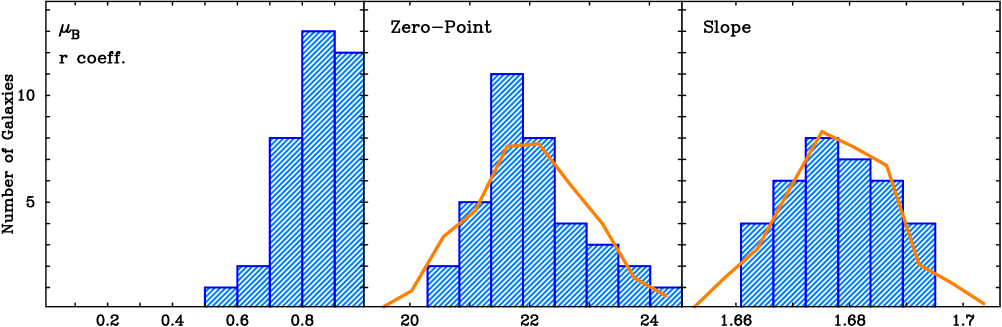
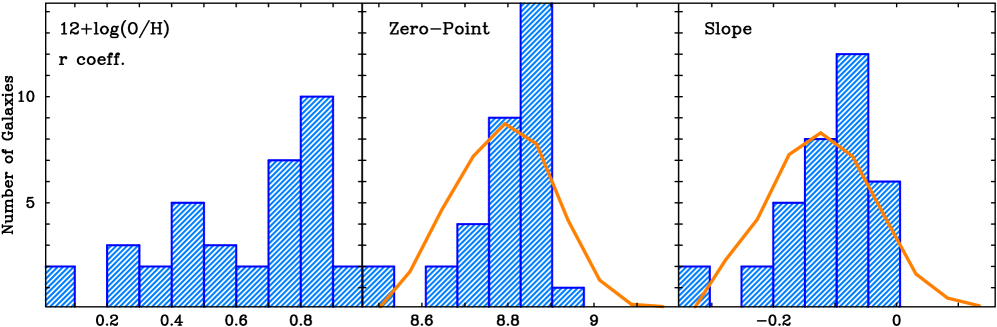
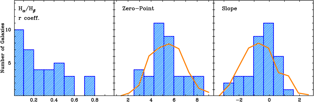
Figure 10: Summary of the analysis of the gradients of a set of physical properties of the H ii regions in the considered galaxies. Each panel shows, from left to right, (i) the distribution of correlations coefficients of a each of the considered parameter (from top to bottom: the surface brightness, the oxygen abundance and the dust attenuation) with respect to the radial distance; (ii) the distribution of the zero-points of the linear regression and (iii) the distribution of the slope of the same regression. The orange solid line represents, for each of the last two histograms, the expected histogram in case of a Gaussian distribution of the data, assuming the mean and standard-deviation of the distribution of each analyzed parameter, and sampled with same bins.

7.1.2 Mass-Metallicity Relation

Stellar mass and metallicity are two of the most fundamental physical properties of galaxies. Both are metrics of the galaxy evolution process, the former reflecting the amount of gas locked up into stars, and the later reflecting the gas reprocessed by stars and any exchange of gas between the galaxy and its environment. Understanding how these quantities evolve with time and in relation to one another is central to understanding the physical processes that govern the efficiency and timing of star formation in galaxies.

Tremonti et al. (2004) found a tight correlation between stellar mass and gas-phase metallicity (MZR) spanning over 3 orders of magnitude in stellar mass and a factor of 10 in metallicity. This correlation has been interpreted as a direct evidence of the anticorrelation between metal loss with baryonic mass, and the ubiquity of galactic winds and their efficiency in removing metals from low-mass galaxies. Additional interpretations consider that the observed mass-metallicity relation is due to a more general relation between stellar, gas-phase metallicity and star formation rate (Lara-López et al., 2010; Mannucci et al., 2010).

Despite the strength of the considered correlation and how it matches with our current understanding on galaxy evolution, there are a few caveats on how the MZR is derived: (i) The oxygen abundance used by Tremonti et al. (2004) was derived assuming a Bayesian approach based on simultaneous fits to all the most prominent lines assuming the results provided by photoionization models. However, as explained before these methods systematically overestimate by 0.2–0.4 dex the oxygen abundances derived using the Te-based calibrations(Lopez-Sanchez et al., 2012); (ii) the calibrator was derived for H ii regions, but applied to integrated apertures in galaxies. Although it is widely used, it is is not firmly tested if this procedure is valid; (iii) the apertures of the considered spectra cover a different optical extent for each galaxy, due to the fixed aperture of the SDSS fiber spectra (3$\arcsec$).

So far, there has been no major effort to test the reported relation using spatially resolved spectroscopic information, like the one provided by the current analysis. The number/statistics of our analysis, galaxy-by-galaxy, is reduced, and we can only test if our results are consistent with the derived relation. However, it will be a first step towards a stronger statistical result, that could be provided with the large sample currently under observation by the CALIFA survey (Sánchez et al., 2011).

We derive the luminosity mass of the considered galaxies using the integrated $B$-band magnitudes, $B-V$ colors and the average mass-luminosity ratio ($M/L$) described in Bell & de Jong (2001). This derivation is less accurate than the one described in Tremonti et al. (2004). However, it should be enough for the purpose of this analysis, considering that the derived $M/L$ has an expected scatter of $\sim$0.15 dex (Bell & de Jong, 2001). As an additional cross-check we also derived the dynamical mass. We use the effective radius ($r_{e}$), the maximum rotational velocity ($v_{\rm rot}$) listed in Table 1, and the classical formula :

$$M_{\rm dyn}=\frac{{r_{e}}{v_{\rm rot}}^{2}}{G}.$$ (14)

We note here that this mass is indeed the dynamical mass at a particular radius (roughly twice the effective one), and therefore, the derived values should be taken with caution for any further interpretation. As expected the dynamical mass is slightly larger than the stellar mass, since the first considers the total mass of the galaxy. However, both masses agree within $\pm$0.2 dex for $\sim$90% of the objects. Similar results have been recently reported for the same sort of galaxies, using more sophisticated derivations of the stellar masses (Gerssen et al., 2012). This consistent result strengthens the validity of our derived masses.

Figure 9 shows the distribution of the oxygen abundance at the center of the galaxies vs. the stellar masses described before. The oxygen abundance has been derived extrapolating the radial gradients found for each galaxy (see Sec. 7.2), to the center. For comparison, we estimate the central abundance using the average of the metallicity values within 0.2$r_{e}$, using the O3N2 calibrator, for those galaxies with H ii regions at this distance (20 out of 38). Both values agree within the errors. We prefer to use the extrapolation of the derived gradient, since they have lower dispersion, and they can be derived for more galaxies (i.e., all but MRK 1477). We include in Fig 9 the relation between both quantities derived by Tremonti et al. (2004), corrected for the mismatch between their calibrator and the currently used here (i.e., 0.15 dex). The derived central abundance and stellar masses for the galaxies analyzed here are consistent with this relation, showing a similar distribution: about 75% of the galaxies are located at less than $\sim$1$\sigma$ of the scaled relation.

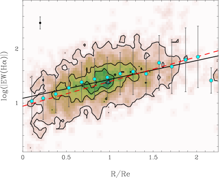
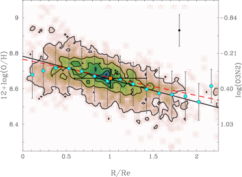
Figure 11: Left panel: Radial distribution of the equivalent width of H$\alpha$ (in logarithm scale of its absolute value), once scaled to the average value at the effective radius for each galaxy. The image and contours show the density distribution of H ii regions in this parameter space. The first contour indicates the mean density, with a regular spacing of four times this value for each consecutive contour. The light-blue solid-circles indicate the mean value (with its corresponding standard deviation represented as error bars), for each consecutive radial bin of $\sim$0.15 R_e. The solid line shows the average linear regression found for each individual galaxy, as listed in Table 8. The red dashed line shows the actual regression found for all the H ii regions detected for all the galaxies. The average error of the equivalent width of H$\alpha$ for the H ii regions represented in this plot is shown by a single error bar located at the top-left side of the panel. Right panel: Similar radial distribution for the oxygen abundance derived using the O3N2 indicator, once scaled to the average value at the effective radius for each galaxy, following the same format. The average error of the derived oxygen abundance (without considering systematic errors) is shown by a single error bar located a the top-right side of the panel. The right-side scale shows the corresponding value for the O3N2 indicator. The solid-orange square indicate the average abundance of the solar neighborhood, at the distance of the Sun to the Milky-Way galactic center (in effective radius).

7.2 Radial gradients

It is well known that different spectroscopic properties of H ii regions show strong variations across the area of disk galaxies. In particular, some of these parameters (e.g., oxygen abundance, EW[H$\alpha$], etc.), show a strong radial gradient, that in average indicates that more evolved, metal rich, stellar populations are located in the center of galaxies, and less evolved, metal poor ones are in the outer ones (e.g. Zaritsky et al., 1994; Rosales-Ortega et al., 2011, and references therein). This observational result is consistent with the our current understanding of the formation and evolution of spiral galaxies (e.g. Tsujimoto et al., 2010, , and references therein). Gas accretion brings gas into the inner region, where it first reaches the required density to ignite star formation. Thus the inner regions are populated by older stars, and they have suffered a faster gas reprocessing, and galaxies experience an inside-out mass growth (e.g. Matteucci & Francois, 1989; Boissier & Prantzos, 1999). Both the extinction-corrected color gradients in nearby galaxies, Muñoz-Mateos et al. (2007), and weak dependence of the mass-size relation with redshift (Trujillo et al., 2004; Barden et al., 2005; Trujillo et al., 2006) support an inside-out scenario for the evolution of disks.

Pure inside-out growth is affected by internal and external events, like bars and/or galaxy interaction and mergers, which induce radial migration. In principle, radial migration affects the stellar populations more strongly, since they are dynamically more susceptible to the effects that produce migration (interactions, bars, etc.). The overall result is a change in the slope of the surface brightness profile and colors of these galaxies (e.g. Bakos et al., 2008). However, gas clumps, like H ii regions, may also be affected (e.g. Minchev et al., 2012). The net effect of these processes is a possible flattening of the radial gradient and/or a truncation at outer regions, where some of these properties (e.g. oxygen abundance) show values that are expected at more inner regions. This change in the slope of the radial gradient of oxygen abundance has been reported by several authors (e.g. Bresolin et al., 2009; Marino et al., 2012; Bresolin et al., 2012). If true, migration is an efficient mechanism to intermix the gas and stellar population properties of galaxies, and even to enrich the intergalactic medium (Sánchez-Blázquez et al., 2009, for a different explanation to the surface-brightness truncation).

Despite of the several different studies describing these observational events, there is a large degree of discrepancy between the actual derived parameters describing the gradients: (i) slope of the gradient; (ii) average value and dispersion of the zero-point and (iii) scale-length of the truncation. In general, this is mostly due to different observational biases and historical methods to perform the analysis: (i) most of the studies lack a proper statistical number of analyzed H ii regions per galaxy; (ii) in many cases the samples cover mostly the outer regions (R$>$R_e), with a lack of H ii regions in the inner ones; (iii) there is no uniform method to analyze the gradients. In some cases the physical scales of the galaxies (i.e., the radii in kpc) are used, (e.g. Marino et al., 2012). In others the scale-length are normalized to the R₂₅ radii, i.e., the radii at which the surface brightness in the $B$-band reach the value of 25 mag/arcsec² (e.g. Rosales-Ortega et al., 2011). Finally, a much more reduced number of studies tries to normalize the scale-length based on the effective radii (described in Sec. 6.1.2). Diaz (1989), in one of the earliest compilations of H ii regions already showed that the effective radius is the best one to normalize the abundance gradients. This is somehow expected since it is directly related with the mass concentration and reflects how fast the gas is recycled in different galaxies. Despite its benefits, it is the least used one, which has produced an ill-defined set of definitions for these gradients. It is important to remember here that both the physical scale of the radial distance and/or the normalized one to an absolute parameter like the $R_{25}$ radius, although they are widely used, could not produce useful gradients to compare galaxy to galaxy, since in both cases the derived gradient is correlated with either the scale-length of the galaxy of its absolute intensity.

7.3 Analysis of gradients galaxy by galaxy

We used our catalogue of H ii regions to characterize the radial gradients of the physical properties of the H ii regions. For each galaxy we derive the correlation coefficient, and the slope and zero-point of a linear regression; for the radial distribution we derived each of the parameters discussed in the previous section. The radial distance is normalized to the effective radius of each galaxy, listed in Table 4. Only those galaxies with a good sampling of the radial distribution of H ii regions have been considered. To do so, we adopted two criteria: (i) the galaxy should comprises more than 30 individual H ii regions, and (ii) there should be equally distributed along the sampled region ($\sim$2.5 $R_{e}$).

Table 8 summarizes the result of this analysis. It includes, for each of the considered parameters, the actual number of galaxies considered($N_{gal}$), the median of the correlation coefficients ($r_{cor}$), with its standard deviation ($\sigma_{r}$), the median zero-point ($med_{a}$), with its standard deviation ($\sigma_{a}$), and the mean error of each individual zero-point ($err_{a}$), together with the median slope ($med_{b}$), its standard deviation ($\sigma_{b}$), and the mean error of each individual derived slope ($err_{b}$). In addition to the physical parameters of the H ii regions discussed in the previous section we have included, for comparison purposes two properties of the underlying stellar population, that are well known to correlate with the radial distance: the $B$-band surface brightness ($\mu_{\rm B}$), and the $B-V$ color. The table is ordered by the strength of the correlation for the physical parameters of the H ii regions.

The overall analysis is illustrated is Fig. 10, where we show the distribution of the correlation coefficients, zero-points, and slopes for each individual galaxy, for three particular parameters: (i) the surface brightness, as an example of a strongly correlated parameter; (ii) the oxygen abundance, i.e., the strongest correlated parameter for the ionized gas; and (iii) the dust extinction, a parameter with no gradient in most of the cases. For highly correlated parameters the mean value, shown in Table 7 is not enough to characterize their behavior.

There are parameters that show a statistically significant correlation with the radial distance ($r_{cor}>$0.5, and $\sigma_{cor}<$0.3). These parameters are the Strömgren radii, the oxygen abundance, the equivalent width of H$\alpha$ and the classical ionization diagnostic line rations ([O iii]/H$\beta$ and [N ii]/H$\alpha$). The first correlation may indicate that the H ii regions are larger towards the center. However, we have to be cautious about this statement, since we do not have a direct estimate of the actual size of the H ii regions, and the Strömgren radii are based on particular radiation equilibrium conditions (Osterbrock, 1989). We need to recall here that since many of our so-called H ii regions, are indeed, H ii aggregates, this radius should be considered as an effective radius. The next two correlations show that the more metal rich and evolved stellar populations are located in the inner regions, in agreement with expectations. The remaining two gradients indicates that in general the strength of the ionization is larger in the outer than in the inner regions. Finally, the ionization parameter shows a weaker trend, in the way that less powerful H ii regions are located in the central areas, while the stronger ones are located in the outer regions. However, this result has to be taken with care, since the correlations are weak and the ionization parameter depends both on the electron density and the number of ionizing photons, which may present also radial gradients.

Finally, there are parameters with little dependence with the radial distance, like the dust attenuation and the electron density. If the radial gradient of the parameters discussed before (e.g., oxygen abundance and/or equivalent width of H$\alpha$) is a consequence of the time evolution of the H ii regions (aging, enrichment, lose of strength and expansion), those later ones are not strongly affected by this overall evolution.

7.4 Universal gradients

For those properties showing a strong correlation, it is equally important to understand if the gradient is universal, within our range of explored parameters. Inspecting the histograms shown in Fig. 10 and the values for the slopes listed in Table 8, we can conclude that all the parameters showing either a clear correlation or a trend show well defined slopes, taking into account the considered errors for the measured parameters. For the equivalent width of H$\alpha$ and the oxygen abundance a Lilliefors-test indicates that the histogram of the slopes of the gradients are consistent with a Gaussian distribution (Lilliefors, 1967). This implies that we can define a characteristic value for the slope and that we do not find a population of galaxies with slopes inconsistent with the normal distribution. To illustrate this result we show in Fig. 11 the radial distribution of two of the parameters with stronger correlation: (i) the equivalent width of H$\alpha$ and (ii) the oxygen abundance. We include all the H ii regions in our catalogue ($\sim$2600). For doing so, a global offset has been applied galaxy by galaxy to normalize the equivalent width and the abundance at effective radius. This offset was derived by subtracting the value derived by the individual regression to the median value listed in Table 8. A new regression is estimated for all the dataset of H ii regions. Both the average regression listed in Table 8 (red dashed-line), and the regression for the full sample (black solid-line), has been included. It is clear that both correlations are very similar, which support our claim that there is a universal slope for the gradient of either the equivalent width and the oxygen abundance when the radial scale is normalized by the effective radius.

Fig. 11 shows that the scatter around the described correlation, $\sim$0.6 dex, is much larger than the average error of each individual measurement, $\sim$0.15 dex, for the case of the equivalent width of H$\alpha$. However, in the case of the oxygen abundances both values are very similar, $\sim$0.2 dex. If we interpret this scatter as a typical coherent scale-length, we can conclude that stellar populations with similar star-formation histories are distributed at a wider radial ranges than the corresponding ionized gas with similar oxygen abundance. Thus, the possible intermix due to radial migrations (or similar effects) affects strongly the stars than the ionized gas, as expected. A larger relative scatter in the properties of the stellar population compared with the oxygen abundance ones was reported even in our Galaxy (e.g. Friel, 1995).

For the particular case of the oxygen abundance, the same caveats expressed in Sect. 7.1.1 have to be taken into account here. We derive the abundance using the O3N2 empirical estimator (Pettini & Pagel, 2004), calibration which has a certain range of validity. Due to that we included the corresponding scale of O3N2 values to illustrate that we are in the range where this calibrator provides reliable results. We repeated the analysis using the R₂₃ calibrator, deriving similar results for the radial gradient. However, there is a larger scatter in this distribution, mostly due to the larger error bar of our derivation of oxygen abundance based on this later method, and the lower number of H ii regions with measured [O ii] $\lambda$3727 emission line ($\sim$50% of the total sample).

Despite these caveats, the main result are valid: i.e., there seems to be a universal radial gradient for oxygen abundance when normalized with the effective radii of the galaxies. This result apparently contradicts previous ones, in which the slope of the radial gradients show a trend on certain morphological characteristics of the galaxies. Vila-Costas & Edmunds (1992) shows that barred spirals have a shallower gradient than non-barred ones. However, we must recall here that this statements are based, in general, in gradients on physical scales (i.e. dex kpc^-1), not in normalized ones. A slight decrease in the scatter between the different slopes is appreciated by Vila-Costas & Edmunds (1992) and Diaz (1989), when the scale-length is normalized by the disk-scale, which agrees with our results. We conjecture that both results would come into agreement if the size-luminosity/morphological type relation was considered.

In order to make an independent cross-check we analyzed the distribution of gradients among our galaxies for barred (10 galaxies) and un-barred ones (28 galaxies). No significant difference is found between the distributions, or between any of them and the one comprising the full sample of galaxies; on the basis of a $t$-test analysis, the probability of being different was 63.1% in the worst case. In addition to this test we repeated the comparison for those galaxies with and without well defined spiral arms (see Table 3). The nature of flocculent spirals is still unclear, although the star formation in these galaxies (and therefore, the H ii regions) may not be connected with density waves, but rather with differentially rotating galactic disks (e.g. Efremov et al., 1989). They could be produced also due to gravitational instabilities in the stars due to interactions (e.g. Toomre, 1964). We found no differences among the distributions of slopes for both kind of galaxies.

Finally, for the Grand Design galaxies (i.e., those galaxies with two clearly defined spiral arms listed in Table 3), we repeated the analysis of the gradients for the H ii regions located at each spiral arm. Despite of the lower number statistics, we found not significant difference between the gradients for each spiral arm.

Fig. 11 shows that for the spatial scale which is well sampled by our catalogue of H ii regions (r$<2$r_e), the mean value of the analyzed properties follow the described distribution. For radii larger than $\sim$2 effective radii, the mean abundance and H$\alpha$ equivalent width seem to be slightly offset, with values compatible with more inner regions ($\sim 1$ r_e). Although this seem to agree with previous results reporting a flattening on the oxygen abundance, and even with the migration as a possible explanation, we have to take this result with a lot of caution. There is just a hand-full of H ii regions sampled by our catalogue in this spatial regime (less than a 1%), and therefore the result is not significant. On the other hand, it seems that there is a decrease of mean oxygen abundance in the inner regions of the galaxies ($<$0.3 r_e), compared with the expected value extrapolating the reported correlation. This decrease is not due to the abundance indicator used, since we detect it using either O3N2 or R₂₃ one. Indeed, this decrease was already detected in individual galaxies, like in NGC 628 (Sánchez et al., 2011; Rosales-Ortega et al., 2011).

We explored the possibility of a statistical origin of this effect, by analyzing the distribution of oxygen abundance galaxy by galaxy. However, we found that this decrease is present in 20 of the 28 galaxies with H ii regions detected in the central region. A lower slope in the abundance gradient may induce this effect. However, we found no significant difference in their gradients, with respect to the average values.

Finally, we have explored which would be the actual location of the solar neighborhood in the proposed abundance gradient shown in Fig. 11. For the distance of the Sun to the center of the Milky way we adopted the value deduced by Eisenhauer et al. (2003), of 7.94$\pm$0.42 kpc. The value of the disk scale-length, and therefore the effective radius, is still controversial, with large discrepancies between different results. The more likely value is $\sim$4.5 kpc (i.e., $r_{e}\sim$7.6 kpc), although a dispersion larger than 1 kpc is expected (van der Kruit & Freeman, 2011). Therefore the Sun would be at $\sim$1.1 effective radius of the Galactic center. We note that the abundance in the solar neighborhood is also under debate (Asplund, 2007). The current convention is that it is around $\sim$8.7, with a dispersion of $\sim$0.2 dex (Asplund et al., 2006). Adopting this scale-length and abundance the actual location of the solar neighborhood would be just at the average location from our derive radial gradient (orange square in Fig. 11). Considering that the oxygen abundance has been scaled to the average value at the effective radius, it is interesting to note that our galaxy behaves as the average for typical spiral galaxies.

8 Summary and Conclusions

In this article we have analyzed the H ii regions of a sample of 38 nearby galaxies. The sample has been constructed selecting the almost face-on spiral galaxies presented in Paper I, and similar ones extracted from the PINGS survey Rosales-Ortega et al. (2010). In both cases, the galaxies have been observed using IFS, using the same instrument and sampling similar wavelength ranges with similar resolutions. The IFS data cover most of the optical extension of these galaxies, up to $\sim$2-2.5 effective radii, with enough S/N for the purpose of this study.

We presented HIIexlorer, an automatic method to detect and segregate H ii regions/aggregations based on the contrast of the H$\alpha$ intensity maps extracted from IFS datacubes. Once detected, the procedure provides us with a segmentation map that is used to extract the integrated spectra of each individual H ii region. The method has been compared successfully with other codes available in the literature for NGC 628, the largest galaxy (in projected size) included in the sample.

In total, we have detected 3107 H ii regions, 2573 all of them with good spectroscopic information (i.e. $\sim$60 H ii regions per galaxy). This is by far the largest nearby, 2-dimensional spectroscopic survey presented for this kind of regions up-to-date. Even more, our selection criteria and dataset guarantee that we cover the galaxies in an unbiased way, regarding the spatial sampling. Therefore, the final sample is well suited to understand the spatial variation of the spectroscopic properties of H ii regions in this kind of galaxies.

A well-tested automatic decoupling procedure has been applied to remove the underlying stellar population, and to derive the main properties (intensity, dispersion and velocity) of the strongest emission lines in the considering wavelength range (covering from [O ii] $\lambda$3727 to [S ii] $\lambda$6731). A final catalogue of the spectroscopic properties of these regions has been created for each galaxy. Additional information regarding the morphology, spiral structure, gas kinematics, and surface brightness of the underlying stellar population has been added to each catalogue. In particular, a detailed analysis of the number and structure of the spiral arms has been presented, associating each H ii region to the nearest spiral arm, and classifying them among inter-arms and intra-arms ones. This analysis is highly experimental, and its main aim is to understand asymmetries in the spiral distribution of H ii regions. To our knowledge this is the first time that an H ii region catalogue is provided with two dimensional information and linked to the spiral structure and intra-arm association. The full capabilities of the derived catalogues will be presented in subsequent articles.

In the current study we focused on the understanding of the average properties of the H ii regions and their radial distributions. Among the analyzed properties we include: (1) the equivalent width of H$\alpha$, (2) the amount of dust attenuation (A_V), (3) the most widely used diagnostic line ratios ($\frac{[@series{\mathbf{O\,\mathsc{iii}}}]}{H\beta}$ and $\frac{[@series{\mathbf{N\,\mathsc{ii}}}]}{H\alpha}$), (4) the ionizing parameter (U), (5) the oxygen abundance (O/H), (6) the effective Strömgren radius and (7) the electron density.

We derive the following results:

1. There is statistically significant change in the ionization conditions across the field of view. The fraction of H ii regions affected either by AGNs, shocks or post-AGB stars is much larger for the central regions ($r<0.25r_{e}$), than in the outer ones.

2. The average abundances for the central regions are comparable with the mass-metallicity relation derived by Tremonti et al. (2004). This is particularly important considering that both the technique to derive the stellar masses and the central metallicities (including the adopted calibrator) are different. The fully independent confirmation of the proposed relation through integral field spectroscopy is particularly important as aperture biases can be virtually eliminated.

3. The oxygen abundance and the equivalent width of H$\alpha$ present a radial gradient that, statistically, has the same slope for all the galaxies in our sample, when normalized to the effective radius. The derived slopes for each galaxy are compatible with a Gaussian random distribution and are independent of the morphology of the analyzed galaxies (barred/non-barred, grand-design/flocculent).

4. Other properties show no gradient but seem to vary across each galaxy, and galaxy by galaxy (like the electron density), without a clear characteristic value, or they are well described by the average value either galaxy by galaxy or among the different galaxies (like the dust attenuation).

The H ii regions catalogues of this analysis will be made publicly available for a better use on the astronomical community (see Appendix A and ftp://ftp.caha.es/CALIFA/early_studies/HII/tables/ ).

Appendix A Catalogues of the H ii regions

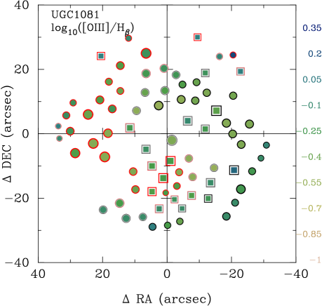
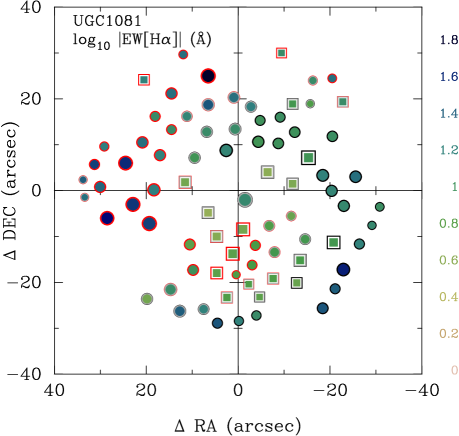
Figure 12: Left-panel: Spatial distribution of the [O iii]/H$\beta$ line ratio along the spatial extension of the UGC 1081 galaxy, derived from the analysis of the H ii regions. Each symbol corresponds to a H ii region, its filling color corresponding to the shown parameter, scaled as displayed in the right-size color-table. Red symbols correspond to H ii regions associated with arm 1, and black ones correspond to those associated with arm 2 (where the indexing of the arms was selected in arbitrary way). Grey symbols represent H ii regions without a clear association with a particular arm, following the criteria described in Sect. 5. The circles represent those H ii regions below the Kauffmann et al. (2003) demarcation line in the BPT diagram shown in Fig. 7, and the squares corresponds to those ones located in the intermediate region between that line and the Kewley et al. (2001) one. The size of the symbols are proportional to the H$\alpha$ intensity. Right-panel: Similar spatial distribution for the absolute value of the equivalent width of H$\alpha$ in logarithm scale. Symbols are similar to those described for the left panel.

The results of the overall analysis on the properties of the H ii regions is compiled in three different catalogues per galaxy, each of them comprising different information. The nomenclature of each catalogue is table.HII.TYPE.GALNAME.csv (for the coma separated version) or table.HII.TYPE.GALNAME.txt (for the space separated ones), where TYPE correspond to each of the following types: coords (coordinates of the H ii regions), flux (fluxes of the stronger emission lines) or EW (equivalent width of the stronger emission lines). GALNAME corresponds to the galaxy name as listed in Table 1.

The catalogues are stored in the CALIFA public ftp server:

ftp://ftp.caha.es/CALIFA/early_studies/HII/tables/ The content of each table is described in the following sections.

A.1 coords tables

They include all the information regarding the location of each H ii region within the galaxy, and additional information regarding their relation with the galaxy morphology, kinematics and the H$\alpha$ luminosity. The tables have the following columns:

1. ID, unique identifier of the H ii region, including the name of the galaxy (NAME) and a running index (NN), in the form: NAME-NNN.

2. RA, the right ascension of the H ii region.

3. DEC, the declination of the H ii region.

4. Xobs, the relative distance in right ascension to the center of the galaxy, in arcsec.

5. Yobs, the relative distance in declination to the center of the galaxy, in arcsec.

6. Xres, the deprojected and derotated distance in the X-axis from the center, in kpc.

7. Yres, the deprojected and derotated distance in the Y-axis from the center, in kpc.

8. R, the deprojected and derotated distance to the center, in kpc.

9. Theta, the deprojected position angle of the H ii region, in degrees.

10. N_Arm, the ID of the nearest spiral arm.

11. Inter_Arm, a flag indicating if the H ii region is most probably associated to a particular arm, 1, or most likely an inter-arm region, 0.

12. D_min-Arm, the minimum distance in arcsec to the nearest spiral arm.

13. D_Arm, the spiralcentric distance, i.e., the distance in arcsec along the nearest spiral arm.

14. Theta_Arm, the angular distance in degree to the nearest spiral arm.

15. vel_Hα, the H$\alpha$ rotational velocity, in km s^-1.

16. e_vel_Hα, error of the H$\alpha$ rotational velocity, in km s^-1.

17. log10(L_Hα), decimal logarithm of the dust corrected luminosity of H$\alpha$, in using of Erg s^-1.

18. e_log10(L_Hα), error of the decimal logarithm of the dust corrected luminosity of H$\alpha$, in using of Erg s^-1.

A.2 flux tables

They comprise the fluxes and ratios of the stronger emission lines detected in each H ii region, as derived from the analysis described in Sect. 6.1. They include the following columns:

1. ID, unique identifier of the H ii region, described in the previous section.

2. Flux_Hβ, observed flux of H$\beta$, in units of 10^-16 erg s^-1 cm^-2.

3. e_Flux_Hβ, error of the observed flux of H$\beta$, in units of 10^-16 erg s^-1 cm^-2.

4. rat_OII_Hb , [O ii] $\lambda$3727/H$\beta$ line ratio.

5. e_rat_OII_Hb, error of the [O ii] $\lambda$3727/H$\beta$ line ratio.

6. rat_OIII_Hb, [O iii] $\lambda$5007/H$\beta$ line ratio.

7. e_rat_OIII_Hb, error of the [O iii] $\lambda$5007/H$\beta$ line ratio error.

8. rat_OI_Hb, [O i] $\lambda$6300/H$\beta$ line ratio.

9. e_rat_OI_Hb, error of the [O i] $\lambda$6300/H$\beta$ line ratio.

10. rat_Ha_Hb, H$\alpha$/H$\beta$ line ratio.

11. e_rat_Ha_Hb, error of the H$\alpha$/H$\beta$ line ratio.

12. rat_NII_Hb, [N ii] $\lambda$6583/H$\beta$ line ratio.

13. e_rat_NII_Hb, error of the [N ii] $\lambda$6583/H$\beta$ line ratio.

14. rat_He_Hb, HeI 6678/H$\beta$ line ratio.

15. e_rat_He_Hb, error of the HeI 6678/H$\beta$ line ratio.

16. rat_SII 6717_Hb, [S ii] $\lambda$6717/H$\beta$ line ratio.

17. e_rat_SII 6717_Hb, error of the [S ii] $\lambda$6717/H$\beta$ line ratio.

18. rat_SII 6731_Hb, [S ii] $\lambda$6731/H$\beta$ line ratio.

19. e_rat_SII 6731_Hb, error of the [S ii] $\lambda$6731/H$\beta$ line ratio.

20. BPT_type, flag indicating the location of the ionized gas region in the classical BPT [O iii]/H$\beta$ vs. [N ii]/H$\alpha$ diagnostic diagram shown in Fig. 7, with the following values: (0) location undetermined, due to the lack of any of the required line ratios with sufficient S/N for this analysis; (1) region located below the Kauffmann et al. (2003) demarcation line, i.e., corresponding to a classical star-forming H ii region; (2) region located in the intermediate area within the Kauffmann et al. (2003) and the Kewley et al. (2001) demarcation lines, i.e.; (3) region located above the Kewley et al. (2001) demarcation line, i.e., corresponding to the area expected from being ionized by an AGN and/or a shock.

A.3 EW tables

They comprise the equivalent width, in Angstroms, of the stronger emission lines detected in each H ii region, as derived from the analysis described in Sect. 6.1. They include the following columns:

1. ID, unique identifier of the H ii region, described in the previous section.

2. EW_OII, equivalent width of [O ii] $\lambda$3727.

3. e_EW_OII, error of the equivalent width of [O ii] $\lambda$3727.

4. EW_Hbeta, equivalent width of the H$\beta$ emission line.

5. e_EW_Hbeta, error of the equivalent width of H$\beta$.

6. EW_OIII, equivalent width of [O iii] $\lambda$5007.

7. e_EW_OIII, error of the equivalent width of [O iii] $\lambda$5007.

8. EW_OI, equivalent width of [O i] $\lambda$6300.

9. e_EW_OI, error of the equivalent width of [O i] $\lambda$6300.

10. EW_Halpha, equivalent width of H$\alpha$.

11. e_EW_Halpha, error of the equivalent width of H$\alpha$.

12. EW_NII, equivalent width of [N ii] $\lambda$6583.

13. e_EW_NII, error of the equivalent width of [N ii] $\lambda$6583.

14. EW_SII, equivalent width of the [S ii] $\lambda\lambda$6717,6731 doublet.

15. e_EW_SII, error of the equivalent width of the [S ii] $\lambda\lambda$6717,6731 doublet.

An example of the use of the parameters listed in these tables is shown in Fig. 6, and in the analysis performed in Sect. 6.1.2. Fig. 12 shows an example of the two dimensional distribution of the properties included in the described catalogues, which makes use of the many different properties studied for the H ii regions.

Appendix B Empirical correction of the [N ii] contamination in H$\alpha$ narrow band images

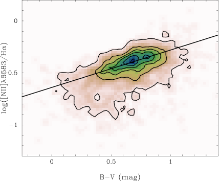
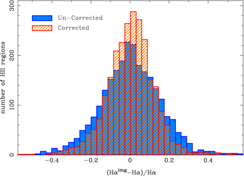
Figure 13: left panel: Distribution of the [N ii]/H$\alpha$ line ratio along the $B-V$ color for all the detected H ii regions. The image and contours show the density distribution in this space of parameters. The first contour is at the mean density, with a regular spacing of four times this value for each consecutive contour. The solid line shows the actual regression found between the two represented parameters. right panel: Histograms of the relative difference between the H$\alpha$ intensity derived from the narrow band images described in Sect. 3, and the ones derived from the fitting technique over the extracted spectra, described in Sect. 6.1, before (blue-solid histogram) and after (red-shaded histogram) applying the correction from the [N ii] contamination based on the correlation shown in the left-panel.

The H$\alpha$ luminosity observed in spiral and irregular galaxies is believed to be a direct tracer of the ionization of the inter-stellar medium (ISM) by the ultraviolet (UV) radiation which is produced by young high-mass OB stars. Since only high-mass, short-lived, stars contribute significantly to the integrated ionizing flux, this luminosity is a direct tracer of the star formation rate (SFR), independent of the previous star formation history. This is why dust-corrected H$\alpha$ luminosity is one of the most widely used observables to derive SFR in galaxies.

Among the several methods used to derive the H$\alpha$ luminosity and its distribution across the optical extension of the galaxies, narrow-band image is by far the cheapest one in terms of telescope time and complexity. Thus, it is the most frequently used too (e.g., James et al. 2004; Pérez-González et al. 2003). The technique is rather simple: (i) the galaxy is observed using both a narrow-band filter centered at the wavelength of H$\alpha$ and a broader filter covering a wider range around the same wavelength range; (ii) The broad-band image is used to correct for the underlying continuum and provide a relative flux calibration of the continuum subtracted narrow-band image; (iii) by performing a flux calibration of the broad-band image it is possible to have an accurate calibration of the decontaminated H$\alpha$ emission map.

One of the major limitations of narrow-band H$\alpha$ imaging is contamination by the [N ii] line doublet, which can hardly be derived from a single narrow-band imaging (e.g. James et al. 2005). Most frequently used narrow-band filters have a width of $\sim$50-80Å, and in most of the cases the emission from the [N ii] $\lambda\lambda$6548,6583 contaminate the derived H$\alpha$ emission map, and therefore, the derived H$\alpha$ luminosity and SFR. Despite of the fact that the [N ii]/H$\alpha$ line ratio present a strong variation across the field for star-forming galaxies (e.g. Sánchez et al. 2011, and Fig 7), it is generally assumed an average correction.

The most commonly used corrections for entire galaxies are those derived by Kennicutt (1983) and Kennicutt & Kent (1983). Spectrophotometric [N ii]/H$\alpha$ ratios of individual extragalactic H ii regions from the literature (see Kennicutt & Kent 1983 and references therein) were compiled from 14 spiral galaxies (mostly of type Sc) and 7 irregular galaxies. The average H$\alpha$/(H$\alpha$ + [N ii]) ratio was found to be fairly constant, spanning the ranges 0.75$\pm$0.12 for the spirals, and 0.93$\pm$0.05 for the irregulars (Kennicutt 1983). In terms of the ratio [N ii]-total/H$\alpha$ this corresponds to a median value of 0.33 for spirals and 0.08 for irregulars. These values were calculated by finding the [N ii]-total/H$\alpha$ ratio of the brightest H ii regions, averaging for each galaxy and then determining the mean value for spiral and irregular types. This implicitly assumes that all H ii regions have the same proportion of [N ii]-total to H$\alpha$ emission as those regions measured. We have already illustrated that this may not be the case in general, e.g., Fig. 7. However, recent results show that the total integrated spectra of galaxies may have a stronger [N ii] emission than the one reported before, with a large variation line ratios for different galaxy types Kennicutt (1992).

Jansen (2000) already showed that there is a trend of the average [N ii]/H$\alpha$ ratio with galaxy luminosity. In their study, the lines ratios for galaxies brighter than M_B = $-$19.5 are in agreement with the values found by Kennicutt (1992), but fainter than this a striking trend is seen towards much lower values of this ratio. A similar trend is found by Gavazzi et al. (2004).

To our knowledge the only attempt to make a correction across the optical extension of each galaxy is the one introduced by James et al. (2004). In this study they used the spatial distribution of the [N ii]/H$\alpha$ line ratio, instead of an average correction for all the entire galaxy. However, their estimations of the distribution of the line ratio are based on physical principles rather than in direct measurements.

Making use of our extensive catalogue of individual emission line regions, we have explored possible empirical corrections that allow us to perform spatially resolved corrections across the optical extension of each individual galaxy. For doing so we correlated the measured [N ii]/H$\alpha$ line ratios for each individual region with different parameters easy to address using broad-band photometry, like the H$\alpha$ intensity, $B$ and $V$-band magnitudes, $B-V$ colors and radial distance relative to the effective radius.

Among the different explored linear relations, the one with stronger correlation coefficient ($r\sim$0.5), and better defined zero-point and slope, was the one with the $B-V$ color:

$$\log_{\rm 10}([@series{\mathbf{N\,\mathsc{ii}}}]/H\alpha)=-0.64_{\pm 0.20}+0.36_{\pm 0.18}(B-V)$$ (15)

Fig. 13, left panel, shows the distribution of [N ii]/H$\alpha$ line ratios along the $B-V$ color for all the detected H ii regions. The image and contours show the density distribution in this space of parameters, together with a solid line showing the best fitted linear regression described before. This relation can be used as a simple proxy of the [N ii]/H$\alpha$ line ratio, and used to decontaminate the described H$\alpha$ narrow-band images.

We applied the proposed correction to the H$\alpha$ narrow-band images described in Sect. 3, to demonstrate its improvement over a classical single correction over the entire galaxy. We derive for each detected H ii region the corresponding flux in the H$\alpha$ narrow-band images, using the segmentation maps provided by HIIexplorer (H$\alpha^{\rm img}$). Then, we obtain the relative difference between this contaminated flux and the real H$\alpha$ flux measured using the fitting procedure describe in Sect. 6.1. The mean value of this difference is $\sim$0.28$\pm$0.19, which is consistent with the typical average correction found in the literature (e.g., Kennicutt 1983). Fig. 13, right panel, shows a solid-blue histogram of the relative difference between the H$\alpha$ flux derived from the narrow-band images, and the ones derived using the emission line fitting procedure after applying this average correction.

The derived correction is then applied on the same data using a iterative processes. In each iteration the $B-V$ color is used to guess the [N ii]/H$\alpha$ line ratio. This ratio, together with the decontaminated H$\alpha$ flux derived from in the previous iteration, is used to derive the [N ii] intensity. Finally, this intensity is subtracted to the original contaminated H$\alpha^{\rm img}$ intensity to derive a new decontaminated flux. For the first iteration it is assumed that the intensity decontaminated by the average correction is a good starting estimation of the H$\alpha$ flux. After three iterations the decontaminated H$\alpha$ flux converge with a few percent. Fig. 13, right panel, shows a hashed-red histogram of the relative difference between the the H$\alpha$ flux derived from the narrow-band images, and the ones derived using the emission line fitting procedure after applying the proposed correction. It is clear that the new histogram has a lower dispersion that the previous one, with a standard deviation of $\sim$0.15. The proposed correction improves the accuracy of the derived H$\alpha$ intensity by a a $\sim$60%, in average.

The effect of this correction is stronger when analyzing the spatial distribution of the H$\alpha$ emission and/or the relative strength of the SFR. As we already indicated the [N ii]/H$\alpha$ ratio tends to decrease with the radius. Therefore, an average correction would overestimate the H$\alpha$ emission and the SFR in the inner regions, and underestimate it in the outer ones. Indeed, some authors have corrected the image-based H$\alpha$ fluxes for [N ii] contamination using available spectroscopical data of selected H ii regions within the galaxy (e.g. López-Sánchez & Esteban 2008).

So far, we did pay no attention to the possible physical connections between the explored parameters. The described relation may indicate a physical connection between the conditions of the ionized gas and the ionizing stellar population, or between both of them and a third parameter not considered here. A possible origin of this connection could be a co-evolution of both components of the H ii regions. The study of this connection, that we will address in future works, is beyond the scope of the current analysis.