Active-to-absorbing state phase transition in the presence of fluctuating environments: Weak and strong dynamic scaling

Abstract

We investigate the scaling properties of phase transitions between survival and extinction (active-to-absorbing state phase transition, AAPT) in a model, that by itself belongs to the directed percolation (DP) universality class, interacting with a spatio-temporally fluctuating environment having its own non-trivial dynamics. We model the environment by (i) a randomly stirred fluid, governed by the Navier-Stokes (NS) equation, and (ii) a fluctuating surface, described either by the Kardar-Parisi-Zhang (KPZ) or the Edward-Wilkinson (EW) equations. We show, by using a one-loop perturbative field theoretic set up, that depending upon the spatial scaling of the variance of the external forces that drive the environment (i.e., the NS, KPZ or EW equations), the system may show weak or strong dynamic scaling at the critical point of active to absorbing state phase transitions. In the former case AAPT displays scaling belonging to the DP universality class, whereas in the latter case the universal behavior is different.

I Introduction

The simple epidemic process with recovery or the Gribov process grib1 ; grib2 serves as an example of a prototypical nonequilibrium phase transition. It, also formally known as the Reggeon field theory rft1 ; rft2 ; rft3 , is a stochastic multiparticle process that describes the essential features of local growth processes of populations in a uniform environment near their extinction threshold popdyn2 ; popdyn3 and belongs to the Directed Percolation (DP) universality class. For recent reviews see Refs. hinrev ; uwe-hans-review . A simple realization of the DP process is the predator-prey cellular automaton models. These models display nonequilibrium active to absorbing state phase transitions (AAPT) separating active from inactive or absorbing states due to competitions between spontaneous particle decay (death) and particle production (birth) processes. In these models for certain parameter values, the steady state density is zero, i.e., the species gets extinct. By definition, once reached an absorbing configuration, the system can not escape from these configurations marro . Experimental realizations of DP universality has been reported in Ref. chate recently, where transitions between two topologically different turbulent states of nematic liquid crystals in their electrohydrodynamic convection regimes were observed. Ref. chate measured the relevant scaling exponents with high accuracy and found them to belong to the DP universality class. The critical behavior of the AAPT hinrev depends on the conservation laws in the dynamics and the underlying symmetry. It has been conjectured in the form of the Directed Percolation Hypothesis popdyn3 ; dpuniv that in the absence of any special symmetry or conservation laws the AAPT belongs to the DP universality class as long as the system has a single absorbing state. In a more realistic situation, the spreading process in DP can also be long ranged. For example, consider infecting agents being advected by a local velocity field (e.g., parasites being carried in a wind flow in an ecological system). To analyze such a situation, Ref. grass20 introduced a variation of the epidemic process with an infection probability distribution that decays with the distance $r$ as a power law. Such long range DP models have analyzed in details numerically hin-how , as well as analytically by using field theoretic methods field1 ; field2 . In particular, Ref. field2 demonstrated four possible set of universal exponents for the long range DP problem, corresponding to four different pairs of (renormalization group) fixed point values for the two coupling constants in the model, reflecting several possible universal scaling behavior. Ref. field2 enumerates the critical exponents at each of the fixed points and their stabilities. More recently, Ref. antonov discusses the effects of temporally $\delta$-correlated multiplicative noises on the universal properties of the AAPT. They discussed the condition under which the usual DP universality class becomes unstable with respect to perturbations by the multiplicative noises.

In the usual models belonging to the DP universality, the parameters defining the models are taken to be constants. Thus they represent a constant (non-fluctuating) environment. In this article we discuss the general question of how interactions with a spatially and temporally fluctuating environment affects the statistical properties of a percolating agent or the density of a near-extinct population $\phi$ at the critical point of an AAPT belonging to the DP universality class, by coupling the environmental fluctuations explicitly with the growth process. In order to address this question, we consider two different cases of fluctuating environments separately, namely, (i) a randomly stirred fluid, described by the Navier-Stokes (NS) equation, and (ii) a fluctuating surface, modeled by the Kardar-Parisi-Zhang (KPZ) or Edward-Wilkinson (EW) equations. We do not consider any feedback of $\phi$ to the environment, i.e., the time evolution of the environment is autonomous. In all the cases, the coupling with the environment is nonlinear. Further we drive the environment (i.e., the NS, KPZ or EW equations) by Gaussian stochastic long-ranged forces with specified variances. Because of our choice for the dynamics of the environment, it itself displays universal spatial and dynamical scaling in the long wavelength limit, with the universality class depending upon the model used. In each of the cases we calculate the relevant scaling exponents at the critical point. The main result that we find is that the scaling behavior of the system near the extinction point of the AAPT depends generally upon the location of the system in the phase space spanned by dimensionality $d$ and a parameter $y$ that characterizes the spatial scaling of the noise correlations in the NS, KPZ or EW models, and depending upon the location in the phase space, the model may exhibit strong dynamical scaling, when the dynamics of the field $\phi$ and the environment are characterized by the same dynamic exponent, or weak dynamical scaling, when the two have different dynamic exponents. Specifically in our model, weak dynamic scaling implies scaling properties of $\phi$ belonging to the DP universality class, where as strong dynamic scaling corresponds to non-DP behavior. It may be noted that AAPT in contact with a randomly stirred velocity field has been considered in Ref. antonov1 . We compare our results and scheme of calculations with Ref. antonov1 later.

Motivations of our work are both theoretical and phenomenological. Our results are similar to those in Ref. field2 , and provides for a mechanism to introduce long range flight in the otherwise local models of epidemic with recovery. Presence of both weak and strong dynamic scaling (in different regions of the phase space) makes it a good candidate to study general issues related to dynamical scaling in NESS. Apart from theoretical motivations, the models and results discussed here are useful in more biologically motivated context. Let us consider the specific example of a bacteria colony (or a biofilm of bacteria) undergoing simple cell division and death in its ordered (nematic or polar) phase. The nematic or polar order parameter being a broken symmetry mode obeys a dynamics that is scale invariant. This should be coupled to the dynamics of the bacteria density, which in addition to the growth decay terms, should have symmetry-allowed couplings with the order parameter field. Moreover, bacteria being living systems, there should be specific nonequilibrium stresses (or active stresses) arising from the continuous energy consumption of the living bacteria. Thus one obtains a coupled model of a density undergoing the extinction transition and a broken-symmetry order parameter field executing scale invariant dynamics. Our results here will help us understanding the interplay between the density field and the order parameter field in determining the universal scaling near the extinction threshold for more realistic naturally occurring systems. The rest of the paper is organized as follows: In Sec. II.1 we discuss the basic DP model and the results from it in some details. Then in Sec. II.2 we discuss the case when the population density is coupled with a randomly stirred fluid described by the NS equation. Within a one-loop DRG approach we analyze the fixed points, calculate the associated scaling exponents determined by the stable fixed points and present a linear stability diagram. In Sec. II.3 we consider the environment to be a fluctuating surface, which is governed either by the KPZ or the EW equations. In all the cases we obtain the relevant scaling exponents by one-loop renormalized perturbative calculations. In Sec. III we summarize and discuss our results.

II Equations of motion

II.1 Directed Percolation model

In order to set up the calculational background of our model, let us briefly revisit the problem of extinction of a single species in a uniform environment and its universal properties near the extinction threshold. As an example, let us consider population dynamics with population growth rate that depends linearly on the local density of the species and death rate that depends quadratically on the local density also undergoing a non-equilibrium active to absorbing state (i.e., species extinction) phase transition whose long distance large time properties are well-described by the DP universality class. In terms of a local particle number density $\phi({\bf x},t)$ and taking diffusive modes into account, the Langevin equation that describes such a population dynamics is given by [see, e.g., Ref. uwe-hans-review ]

$$\frac{\partial\phi}{\partial t}=D\nabla^{2}\phi+\lambda_{g}\phi-\lambda_{d}\phi^{2}+\sqrt{\phi}\zeta,$$ (1)

where $D$ is the diffusion coefficient, $\lambda_{g}$ is the growth rate and $\lambda_{d}$ the decay rate of the density field $\phi$. Stochastic function $\zeta({\bf x},t)$ is a zero-mean, Gaussian distributed white noise with a variance given by

$$\langle\zeta({\bf x},t)\zeta(0,0)\rangle=2D_{2}\delta({\bf x})\delta(t).$$ (2)

The multiplicative nature of the effective noise in Eq. (1) ensures the in-principle existence of an absorbing state ($\phi=0$) in the system. Equation (1) allows us to extract the characteristic length $\xi\sim\sqrt{D/|\lambda_{g}|}$ and diffusive time scale $t_{c}\sim\xi^{2}/D\sim D/|\lambda_{g}|$ on dimensional ground, both of which diverge upon approaching the critical point at $\lambda_{g}=0$. Upon defining the critical exponents in the usual way uwe-hans-review

$$\langle\phi({\bf x},t\rightarrow\infty)\rangle\sim\lambda_{g}^{\beta},\;\;\langle\phi({\bf x},t)\rangle\sim t^{-\alpha}\;(\lambda_{g}=0),\;\;\xi\sim\lambda_{g}^{-\nu},\;\;t_{c}\sim\xi^{z}_{\phi}/D\sim\lambda_{g}^{-z_{\phi}\nu},$$ (3)

we identify the mean-field values

$$\beta=1,\alpha=1,\nu=1/2,\,\,{\mbox{and}},\,\,z_{\phi}=2.$$ (4)

Further, the anomalous dimension $\eta$, which characterizes the spatial scaling of the two-point correlation function, is zero uwe-hans-review . It is, however, well-known that fluctuations are important near the critical point and as a result mean-field values for the exponents are quantitatively inaccurate. In order to account for the fluctuation effects, dynamic renormalization group (DRG) calculations have been performed over an equivalent path integral description of the Langevin Eq. (1) uwe-hans-review . A one-loop renormalized theory with systematic $\epsilon$-expansion, $\epsilon=d_{c}-d$, where the upper critical dimension $d_{c}=4$ for this model, yields uwe-hans-review ,

$$z=2-\epsilon/12,\eta=\epsilon/12\,\,\mbox{and}\,\,{1\over\nu}=2+\epsilon/4.$$ (5)

The DP universality class, characterized by the scaling exponents (5) above, is fairly robust, a feature formally known as the directed percolation (DP) hypothesis dpuniv . Only when one or more conditions of the DP hypothesis are violated, one finds new universal properties. For instance, the presence of long range interactions are known to modify the scaling behavior: Ref. field2 examines the competition between short and long ranged interactions, and identified four different possible phases. Our results assume importance in this backdrop: In our model, long-ranged interactions arise not because of any long range hopping, but due to coupling of the density $\phi$ with an environment, modeled by a randomly stirred fluid or a growing and fluctuating surfaces, all of which in turn are driven by long range noises. It is expected that the presence of these long-range correlated background may affect the universal scaling behavior; our results below confirm this in general.

II.2 Advection of simple epidemic process by a randomly stirred fluid

Here we consider a randomly stirred fluid as a fluctuating environment coupled to the AAPT of a population density near its extinction threshold.

II.2.1 Randomly stirred fluid model

The dynamics of the fluid in the incompressible limit is described by a velocity field $\bf v$ which follows the Navier-Stokes equation landau

$$\partial_{t}v_{i}+\lambda_{1}({\bf v}\cdot\nabla)v_{i}=D_{\nu}\nabla^{2}v_{i}-\frac{\nabla_{i}p}{\rho}+f_{i},$$ (6)

together with the incompressibility condition $\nabla\cdot{\bf v}=0$, which may be used to eliminate pressure in the usual way. Here $p$ the pressure, $\rho$ the density (a constant in the incompressible limit) and $D_{\nu}$ the kinematic viscosity. Parameter $\lambda_{1}$ is a non-linear coupling constant, which does not renormalize in the hydrodynamic limit under mode elimination due to the Galilean invariance of Eq. (6) fns ; yakhot . Function $\bf f$ is the external force required to maintain a driven steady state. A promising starting point for theoretical/analytical studies on homogeneous and isotropic externally stirred fluid is the randomly forced Navier-Stokes model fns ; yakhot , where $\bf f$ is assumed to be a stochastic function which is zero-mean and Gaussian distributed with a variance yakhot

$$\langle f_{i}({\bf q},t)f_{j}({\bf-q},0)\rangle=\delta_{ij}{2D_{1}\over q^{d-4+y}}\delta(t)$$ (7)

in $d$-dimensions, $\bf q$ is a Fourier wavevector, $D_{1}$ is a constant amplitude and $y>0$. We are interested when $d-4+y>0$. Since in this case the variance (7) diverges in the hydrodynamic limit, the force $\bf f$ is said to be long-ranged and is infra red (IR) singular. This is a variant of the Model B (with the identification $y=2-d$) of Ref. fns which was subsequently used in Ref. yakhot to calculate scaling behavior and various universal quantities associated with homogeneous and isotropic $3d$ fluid turbulence. The velocity field shows universal spatial and dynamical scaling independent of the microscopic viscosity and forcing amplitudefoot . These scaling properties are characterized by the roughness exponent $\chi_{v}$ and dynamic exponent $z_{E}$ defined through the definition

$$\langle v_{i}({\bf x},t)v_{i}(0,0)\rangle\sim|{x}|^{2\chi_{v}}f_{v}(|x|^{z_{E}}/t),$$ (8)

where $f_{v}$ is a scaling function. Invariance under the Galilean transformation (see below) yields that the coupling constant does not receive any fluctuation correction in the hydrodynamic limit. A consequence of that is the exact relation between the exponents $\chi_{v}$ and $z_{E}$ yakhot ; jkb : $\chi_{v}+z_{E}=1$. Applications of one-loop DRG to systems with long range noises are more complicated and less controlled than its application in problems of equilibrium critical dynamics yakhot ; jkb ; ronis . Despite the limitations, such calculations are successful in obtaining several useful results on dimensionless numbers and scaling exponents. Due to the infra red singular nature of the bare noise variance (7), the perturbation theory does not generate any fluctuation correction to the bare noise variance (7) which is more singular than it. Consequently, it is assumed to be unrenormalized. Thus in a renormalized perturbation theory, only kinematic viscosity $D_{v}$ undergoes nontrivial renormalization. An explicit one-loop DRG calculation yields

$$z_{E}=2-y/3.$$ (9)

Further, $\chi_{v}=-1+y/3$. Thus for sufficiently high value of $y$, $z_{E}$ may even be less than unity, resulting into turbulent diffusion which is a very efficient way of mixing. In particular, the value $y=d$ in (7) is of particular physical interest, since it corresponds to the famous K41 energy spectrum for the velocity field: One finds for the one-dimensional energy spectrum $E_{v}(q)\sim k^{d-1}\langle|v_{i}({\bf q},t)|^{2}\rangle\sim q^{-5/3}$ in three dimensions.

II.2.2 Extinction transition in contact with a randomly stirred fluid

In the standard models for epidemic with recovery belonging to the DP universality class, the population density field $\phi$ is allowed only to diffuse (apart from local reproduction and death). However in general, such processes (of reproduction and death) may take place in a fluid environment and the local population may get advected in addition to diffusing. Thus they may be called reaction-advection-diffusion systems. For instance, a reaction or birth/death of bacteria may take place in fluid, which in turn may be thermally fluctuating, or may be externally stirred. Here, we find out how the universal properties of standard AAPT are affected when the system is advected by an externally stirred fluid.

The percolating field $\phi$ satisfies the same equation (1), now supplemented by an advective non-linearity:

$$\frac{\partial\phi}{\partial t}+\lambda_{2}{\bf v}\cdot\nabla\phi=D\nabla^{2}\phi+\lambda_{g}\phi-\lambda_{d}\phi^{2}+\sqrt{\phi}\zeta,$$ (10)

Here, $\lambda_{2}$ is a coupling constant, which advectively couples $\phi$ with $\bf v$. Constants $\lambda_{g}$ and $\lambda_{d}$ denote growth and decay rates. Gaussian noise $\zeta$ has the same variance as (2). Redefining coefficients $\lambda_{g}=D\tau$ and $\lambda_{d}=\frac{Dg_{2}}{2}$ for calculational convenience, Eq. (10) may be written as

$$\frac{\partial\phi}{\partial t}+\lambda_{2}{\bf v}\cdot\nabla\phi=D(\nabla^{2}+\tau)\phi-\frac{Dg_{2}}{2}\phi^{2}+\sqrt{\phi}\zeta.$$ (11)

Thus the critical point is now defined by (renormalized) $\tau=0$.

As for the usual DP problem, the system exhibits a continuous phase transition from active to absorbing states as (renormalized or effective) $\tau\rightarrow 0$. The associated universal scaling exponents are formally defined as in (3) above. At the mean-field level the model Eqs. (6) and (11) yield the same mean-field values for the scaling exponents as above in Sec.II.1. Nonlinear couplings $\lambda_{2}$ and $Dg_{2}$, together with the expected large fluctuations near the critical point and multiplicative nature of the long ranged noise with variance (7) are expected to substantially alter the mean-field values of the exponents. Studies of these in-principle require full solution for the field $\phi({\bf x},t)$. Equations (6) and (11) being nonlinear, cannot be solved exactly. Hence perturbative means are necessary. We address this issue systematically via standard implementation of DRG procedure, based on a one-loop perturbative expansion in the coupling constants $\lambda_{2}$ and $Dg_{2}$ about the linear theory. The resulting perturbative corrections to the correlation function may be equivalently viewed as arising from modifications (renormalization) of the parameters and fields in the model Eqs. (6) and (11).

We being with the Janssen-De Dominicis dynamic generating functional bausch corresponding the Langevin equations (6) and (11) together with the corresponding noise variances (2) and (7), which is given by

$${\mathcal{Z}}_{NS}=\int DvD\hat{v}D\phi D\hat{\phi}\exp[S_{NS}],$$ (12)

where $\hat{\phi}$ and $\hat{v}$ are auxiliary fields corresponding to the dynamical fields $\phi$ and $\bf v$ respectively which appear due to elimination of the noises from the generating functional $\mathcal{Z}_{NS}$. The action functional $S_{NS}$ is written as

$$S_{NS}({\bf v},{\bf\hat{v}},\phi,\hat{\phi}) = D_{1}\int\frac{d^{d}k}{(2\pi)^{d}}\int dt\,\hat{v}_{i}\hat{v}_{j}P_{ij}({\bf k})k^{4-y-d}-\int\frac{d^{d}k}{(2\pi)^{d}}\int dt\,\hat{v}_{i}\{\partial_{t}v_{i}-i\frac{\lambda_{1}}{2}P_{ijl}({\bf k})\sum_{\bf q}v_{j}({\bf q})v_{l}({\bf k-q})+D_{\nu}k^{2}v_{i}\}$$

$$-\int\frac{d^{d}k}{(2\pi)^{d}}\int dt\,\hat{\phi}\{\partial_{t}\phi - i\lambda_{2}k_{l}\sum_{\bf q}v_{l}({\bf q})\phi({\bf k-q})+D(k^{2}-\tau)\phi+{Dg_{2}\over 2}\sum_{\bf q}\phi({\bf q})\phi({\bf k-q})-\frac{Dg_{1}}{2}\sum_{\bf q}\hat{\phi}({\bf q})\phi({\bf k-q})\},$$ (13)

where $D_{2}=\frac{Dg_{1}}{2}$, $P_{ij}({\bf k})=\delta_{ij}-{k_{i}k_{j}\over k^{2}}$ is the transverse momentum operator and $P_{ijl}({\bf k})=P_{ij}({\bf k})k_{l}+P_{il}({\bf k})k_{j}$. Note that the last two non-linear terms in (13) do not have the same coupling constant $Dg/2$, unlike the usual DP problem. This is consistent with the lack of invariance of $S_{NS}$ under the rapidity symmetry. The rapidity symmetry of the original DP problem (see, e.g., uwe-hans-review ) is no longer admissible in the present case, since the Navier-Stokes Eq. (6) being a viscous dissipative equation cannot be invariant under time inversion.

Before we present our detailed DRG calculation, let us note the following: Since the dynamics of the randomly stirred fluid is independent of $\phi$, its dynamic exponent $z_{E}$ should be same as that in the absence of any percolating agent. We have $z_{E}=2-y/3$ (see discussions above and the calculations below). Thus if there is a regime characterized by strong dynamic scaling, we should have $z_{\phi}=z_{E}=2-y/3$. In this regime, the nonlinearity of the basic DP process (i.e., coupling constants $g_{1}$ and $g_{2}$) may or may not be relevant in an RG sense, corresponding to what we call LDP (long-range DP) and LR (long range) phases having different static scaling properties (the dynamic exponents are same in LDP and LR phases), characterized by the LDP and LR fixed points (FP), respectively. In contrast, when the coupling constant $\lambda_{2}$ that couples $\phi$ and $\bf v$ is irrelevant in DRG sense, the dynamics of $\phi$ is independent of $\bf v$ and hence $\phi$ displays a dynamics that is identical to the usual DP problem with a dynamic exponent $z_{\phi}=z_{DP}=2-\epsilon/12$. Can there be a phase displaying weak dynamic scaling with $\lambda_{2}$ still being relevant? We expect not; because if $\lambda_{2}$ is indeed relevant (in an RG sense), the the whole action (13) including the coupling term $\hat{\phi}{\bf v}\cdot\nabla\phi$ must be invariant under combined rescaling of space, time and fields characterized by a single set of exponents, i.e., a single dynamic exponent. Thus the assumption of weak dynamic scaling, i.e., the existence of two unequal dynamic exponents, rules out the DRG relevance of $\lambda_{2}$. Finally one may in principle have a phase where all nonlinerities are irrelevant with the $\phi$-field being characterized by the exponents of the linear theory (Gaussian phase) which turns out to be always linearly unstable. Thus, in short, we expect four different phases characterized by four FPs (LR, LDP, DP and Gaussian) and their associated set of exponents. Some of these phases may not be linearly stable. We shall confirm these physically inspired picture through detailed one-loop calculations below. In addition, we calculate all the critical exponents as well.

Equations (6) and (10) are invariant under the Galilean invariance

$${\bf v}\rightarrow{\bf v}+{\bf u}_{0},\,\,\phi\rightarrow\phi,\,\,{\bf x}\rightarrow{\bf x}+{\bf u}_{0}t,\,\,t\rightarrow t,\,\,\frac{\partial}{\partial t}\rightarrow\frac{\partial}{\partial t}.$$ (14)

Invariance of the system under (14) ensures that the coupling constants $\lambda_{1}$ and $\lambda_{2}$ are equal and do not renormalize in the hydrodynamic limit: We henceforth set $\lambda_{1}=\lambda_{2}=\lambda$ below. The role of the (bare or unrenormalized) coupling constants in the ordinary perturbation theory in the present model is played by $u=g_{1}g_{2}$ and $w=\frac{\lambda^{2}D_{1}}{D_{\nu}^{3}}$. In addition, there is a dimensionless number $\theta=D/D_{\nu}$, the Schmidt number which characterizes the ensuing NESS of the AAPT, and is a control parameter of the model. We set up a renormalized perturbative expansion in $\epsilon=4-d$ and $y$ up to the one-loop order. In order to ensure ultra-violet (UV) renormalization of the present model, we are required to render finite all the non-vanishing two- and three-point functions by introducing multiplicative renormalization constants. This procedure is well-documented in the literature, see, e.g., Ref. uwe-book . Here, vertex functions of different orders are formally defined by appropriate functional derivatives of $\Gamma[{\bf v},{\bf\hat{v}},\phi,\hat{\phi}]$ with respect to various fields (dynamical and auxiliary), where $\Gamma$ is the vertex generating functional and the Legendre transform of $\ln Z_{NS}$ uwe-book . In the present model the following vertex functions show primitive divergence at the one-loop level: $(i)\frac{\delta^{3}\Gamma}{\delta v_{i}\delta\hat{v}_{i}},\,(ii)\frac{\delta^{2}\Gamma}{\delta\phi\delta\hat{\phi}},\,(iii)\frac{\delta^{3}\Gamma}{\delta\hat{\phi}\delta\phi\delta\phi},\,(iv)\frac{\delta^{3}\Gamma}{\delta\hat{\phi}\delta\hat{\phi}\delta\phi}.$ Their divergences may be absorbed by introducing renormalization $Z$-factors (see below).

We employ the dimensional regularization scheme to compute the momentum integrals associated with the one-loop vertex function renormalization, and choose $\tau=\mu^{2}$ as our normalization point, where $\mu$ is an intrinsic momentum scale of the renormalized theory. The scaling behavior of the correlation or vertex functions in the hydrodynamic limit may be extracted by finding their dependence on $\mu$ by using the renormalization group (RG) equation, which may in turn be obtained from the one-loop renormalization $Z$-factors. The Galilean invariance of the present model leads to exact Ward identities between certain two- and three-point vertex functions, which yields that the coupling constant $\lambda$ does not renormalize foot2 . Further, since the bare noise variance (7) is IR-singular, perturbation theories do not generate any correction to it which is more singular than it. Thus, the coefficient $D_{1}$ also does not renormalize. Fields $\bf v$ and $\bf\hat{v}$ do not re normalize as well. The renormalized fields and parameters (denoted by a superscript $R$) are defined through the corresponding $Z$-factors as

$$\phi=Z\phi^{R}\,\,,\,\,\hat{\phi}=\hat{Z}\hat{\phi}^{R},\;\;\tau=Z_{\tau}\tau^{R}\,\,,\,\,D=Z_{D}D^{R}\,\,,\,\,g_{1}=Z_{g_{1}}g_{1}^{R}\,\,,\,\,g_{2}=Z_{g_{2}}g_{2}^{R}\,\,,\,\,D_{\nu}=Z_{D_{\nu}}D_{\nu}^{R}.$$ (15)

We perform explicit one-loop calculations in terms of coupling constants $u=g_{1}g_{2}$ and $w=\lambda^{2}D_{1}/D_{\nu}^{3}$. From definition we have $Z_{u}=Z_{g_{1}}Z_{g_{2}}$ and $Z_{w}=Z_{D_{\nu}}^{-3}$. Now absorbing factors of $1/16\pi^{2}$ into these coupling constants i.e, $u\rightarrow u/16\pi^{2}$ and $w\rightarrow w/16\pi^{2}$ we can write down the Z-factors in terms of these scaled coupling constants. Further, since one of the $Z$-factors from the set $Z,\hat{Z},Z_{g_{1}},Z_{g_{2}},Z_{D},Z_{\tau},Z_{D_{\nu}}$ is redundant, we use this freedom to set $Z=\hat{Z}$ without any loss of generality. We obtain

$$Z_{D_{\nu}} = 1-{aw\over y}\mu^{-y},$$ (16)

$$Z = \hat{Z}=1+\frac{u}{8}\frac{\mu^{-\epsilon}}{\epsilon},$$ (17)

$$Z_{D} = 1-\frac{u}{8}\frac{\mu^{-\epsilon}}{\epsilon}-\frac{\lambda^{2}D_{1}}{D_{\nu}D(D_{\nu}+D)}(1-\frac{1}{d})\frac{2}{16\pi^{2}}\frac{\mu^{-y}}{y},$$ (18)

$$Z_{\tau} = 1+\frac{\lambda^{2}D_{1}}{D_{\nu}D(D_{\nu}+D)}(1-\frac{1}{d})\frac{2}{16\pi^{2}}\frac{\mu^{-y}}{y}-\frac{u}{8}\frac{\mu^{-\epsilon}}{\epsilon},$$ (19)

$$Z_{u} = 1+\frac{3u}{2}\frac{\mu^{-\epsilon}}{\epsilon}+4\frac{\lambda^{2}D_{1}}{D_{\nu}D(D_{\nu}+D)}(1-\frac{1}{d})\frac{\mu^{-y}}{y}.$$ (20)

We find from the explicit one-loop results (20) that the $Z$-factors are linear in $u$, $w$ and ${\tilde{w}}=\lambda^{2}D_{1}/[D_{\nu}D(D_{\nu}+D)]$, (but not in $\theta$ directly). Thus the perturbative expansions are in effect expansions in powers of $u$, $w^{R}$ and $\tilde{w}$. Further, $Z_{\theta}=Z_{D}/Z_{D_{\nu}}$ is linear in $\tilde{w}$, but not in $\theta$ itself. In contrast $Z_{\tilde{w}}$ cannot be expressed as a linear function of $\tilde{w}$, along with $u$. In order to simplify the calculation, we make an approximation that $\theta\ll 1$, such that $\tilde{w}=1/(D_{\nu}^{2}D)$. This allows us to write $Z_{\tilde{w}}$ linearly in terms of $\tilde{w}$. We show that, despite our simplifying assumption, we are able to obtain physically meaningful and interesting results which we present below. In the limit of small $\theta$ we get $Z_{\tilde{w}}=Z_{w}Z_{D_{\nu}}/Z_{D}$. Using $Z_{w}=Z_{D_{\nu}}^{-3}$, we can write $Z_{\tilde{w}}=Z_{D_{\nu}}^{-2}Z_{D}^{-1}$. Thus to derive $Z_{\tilde{w}}$ we should find out what $Z_{D}$ is $\theta\ll 1$. It turns out to be (after absorbing a factor of $1/16\pi^{2}$ in the definition of $\tilde{w}$, setting $d=4-\epsilon$ and keeping the lowest order term in $\epsilon$)

$$Z_{D} = 1-{u\over 8\epsilon}\mu^{-\epsilon}-{3\tilde{w}\over 4y}\mu^{-y},$$ (21)

and hence

$$Z_{\tilde{w}}=1+{u\over 8\epsilon}\mu^{-\epsilon}+{2w\over y}\mu^{-y}+{3\tilde{w}\over 4y}\mu^{-y},$$ (22)

where $a=\frac{3}{2}\frac{d-1}{d-2}$. The Wilson’s flow functions can be defined as

$$\zeta_{\phi} = \mu{\partial\over\partial\mu}\ln Z,\,\,\zeta_{\hat{\phi}}=\mu{\partial\over\partial\mu}\ln\hat{Z},\,\,\zeta_{D}=\mu{\partial\over\partial\mu}\ln Z_{D},\,\,\zeta_{\tau}=\mu{\partial\over\partial\mu}\ln Z_{\tau}-2,\,\,\zeta_{D_{\nu}}=\mu{\partial\over\partial\mu}\ln Z_{D_{\nu}},$$ (23)

and the $\beta$-functions as

$$\beta_{u}=\mu{\partial\over\partial\mu}u^{R}\,\,,\,\,\beta_{w}=\mu{\partial\over\partial\mu}w^{R}\,\,,\,\,\beta_{\tilde{w}}=\mu{\partial\over\partial\mu}\tilde{w}^{R}.$$ (24)

The renormalized coupling constants are written as $u^{R}=uZ_{u}^{-1}\mu^{-\epsilon}\,\,,\,\,w^{R}=wZ_{w}^{-1}\mu^{-y}\,\,,\,\,\tilde{w}^{R}=\tilde{w}Z_{\tilde{w}}^{-1}\mu^{-y}$,which for the $\beta$-functions yields

$$\beta_{w}=w^{R}(-y+3aw^{R})\,\,,\,\,\beta_{u}=u^{R}\left(-\epsilon+{3\over 2}u^{R}+{3\over 2}\tilde{w}^{R}\right)\,\,,\,\,\beta_{\tilde{w}}=\tilde{w}^{R}\left(-y+2w^{R}+{3\over 4}\tilde{w}^{R}+{1\over 8}u^{R}\right).$$ (25)

Fixed points of the model are given by the solutions of $\beta_{u}=\beta_{w}=\beta_{\tilde{w}}=0$ which gives us various solutions depending on the different values of the the parameters $u^{R}$, $w^{R}$ and $\tilde{w}^{R}$. The only stable fixed point solution for $w_{R}$ is $w_{R}=y/(3a)$. The different fixed point solutions for $u_{R}$ and $\tilde{w}_{R}$ are as follows:

$$a \rangle \,\,u^{R}=0,\tilde{w}^{R}=0\,\,\,\mbox{ (the trivial Gaussian fixed point)}$$ (26)

$$b \rangle \,\,u^{R}={2\over 3}\epsilon,\tilde{w}^{R}=0\,\,\,\mbox{(the DP fixed point)}$$ (27)

$$c \rangle \,\,u^{R}=0,\tilde{w}^{R}={4\over 9}y\,\,\,\mbox{(LR, long range fixed point)}$$ (28)

$$d \rangle \,\,u^{R}={4\over 5}\epsilon-{8\over 15}y,\tilde{w}^{R}=-{2\over 15}\epsilon+{8\over 15}y\,\,\,\mbox{(LDP, long range DP fixed point)}.$$ (29)

Since by construction $u^{R}$ and $\tilde{w}^{R}$ cannot be negative, from Eq. (29) it is obvious that the non-trivial fixed points may be present in the range $4y\geq\epsilon\geq{2\over 3}y$. For $\epsilon<{2\over 3}y$ the system has fixed points $u^{R}=0$ and $\tilde{w}^{R}={4\over 9}y$ which defines the LR fixed point. For $\epsilon>4y$ the system has fixed points $u^{R}={2\over 3}\epsilon$ and $\tilde{w}^{R}=0$ which defines the DP fixed point. We will see below that these ranges precisely coincide with the region of stability of those fixed points.

The critical exponents are formally related to the Wilson flow functions uwe-hans-review and hence to $u^{R},\,w^{R}$ and $\tilde{w}^{R}$, and are given by

$$\eta_{\phi} = \eta_{\hat{\phi}}=-\zeta_{\phi}={u^{R}\over 8},$$ (30)

$$z_{E} = 2-\zeta_{D_{\nu}}=2-aw^{R},$$ (31)

$$z_{\phi} = 2-\zeta_{D}=2-{u^{R}\over 8}-{3\tilde{w}^{R}\over 4},$$ (32)

$$\nu = -{1\over\zeta_{\tau}}=[2+{3u^{R}\over 8}+{3\tilde{w}^{R}\over 4}]^{-1}.$$ (33)

Thus the different exponents at different regions, defined by $u^{R}$ and $\tilde{w}^{R}$, of the phase space spanned by $\epsilon$ and $y$ are

• At the DP fixed point $({2\epsilon\over 3},0)$, the critical exponents are

  $$\eta_{\phi}=\eta_{\hat{\phi}}={\epsilon\over 12}\,\,,\,\,z_{\phi}=2-{\epsilon\over 12},\,\,\,z_{E}=2-y/3,\,\,,\,\,{1\over\nu}=2+{\epsilon\over 4}.$$ (34)

• At the LR fixed point $(0,{4y\over 9})$, the critical exponents turn out to be

  $$\eta_{\phi}=\eta_{\hat{\phi}}=0\,\,,\,\,z_{\phi}=z_{E}=2-{y\over 3}\,\,,\,\,{1\over\nu}=2+{y\over 3}.$$ (35)

• At the LDP fixed point $({4\epsilon\over 5}-{8y\over 15},-{2\epsilon\over 15}+{8y\over 15})$, the critical exponents are

  $$\eta_{\phi}=\eta_{\hat{\phi}}={\epsilon\over 10}-{y\over 15}\,\,,\,\,z_{\phi}=z_{E}=2-{y\over 3}\,\,,\,\,{1\over\nu}=2+{\epsilon\over 5}+{y\over 5}.$$ (36)

The interesting point to be noted here is that the dynamic exponent $z_{\phi}$ has the same value for both LR and LDP FPs, where has the corresponding static scaling exponents pick up different values. For example, at the LR FP the anomalous dimensions $\eta_{\phi}$ and $\eta_{\hat{\phi}}$, which describe the spatial scaling of the correlation function and the propagator, are zero; hence spatial scaling of the correlation function and the propagator are given by the mean-field analysis (4), where as they pick non-trivial fluctuation corrections at the LDP FP. See Sec. III for more discussions on this.

To analyse the stability of the fixed points we must evaluate the matrix

$$M_{NS}=\left(\begin{array}[]{cc}{\partial\beta_{u}\over\partial u}&{\partial\beta_{u}\over\partial\tilde{w}}\\ {\partial\beta_{\tilde{w}}\over\partial u}&{\partial\beta_{\tilde{w}}\over\partial\tilde{w}}\end{array}\right)$$ (39)

and determine its eigenvalues $\Lambda$ at $u=u^{R}$ and $\tilde{w}=\tilde{w}^{R}$. The condition for infrared stable fixed points is that all the eigenvalues of the stability matrix $M_{NS}$ should be positive:

• At the Gaussian fixed point $(u^{R},\tilde{w}^{R})=(0,0)$ the eigenvalues are $\Lambda=-\epsilon,-{y\over 3}$. As both the eigenvalues are negative the fixed point is unstable.

• At the fixed point $(0,{4\over 9}y)$ the eigenvalues are $\Lambda=-\epsilon+{2\over 3}y,{1\over 3}y$. The stability of this fixed point depends on the condition $\epsilon\leq{2\over 3}y$.

• For the DP fixed point $({2\over 3}\epsilon,0)$ the eigenvalues are $\Lambda=\epsilon,-{1\over 3}y+{1\over 12}\epsilon$. It is stable if $\epsilon\geq 4y$.

• For the fixed point $u^{R}=4\epsilon/5-8y/15,\,\tilde{w}^{R}=8y/15-2\epsilon/15$, eigenvalues are

  $$\Lambda=\left[\frac{11\epsilon}{10}-\frac{2y}{5}\pm\left(\frac{131\epsilon^{2}}{100}+\frac{32y^{2}}{75}-\frac{101y\epsilon}{75}\right)^{1/2}\right]/2=\Lambda_{\pm}$$

  (say). Both eigenvalues are real. One of them $\Lambda_{+}$ is always positive within the window $4y>\epsilon>2y/3$ (this is the window in which this fixed point exists). Since $\mbox{det}M_{NS}=2(3\epsilon-2y)(y-\epsilon/4)/15$ is negative outside this window, the second eigenvalue $\Lambda_{-}$ must change sign when $4y=\epsilon$ or $\epsilon=2y/3$. Thus this fixed point is stable for $4y>\epsilon>2y/3$.

We see that the lines demarcating the regions of stability between the fixed points DP and LDP is given by $\tilde{w}^{R}=0$, which in turn is the same line where the values of the dynamic exponents $z_{\phi}=2-\epsilon/12$ and $z_{\phi}=2-y/3$, corresponding respectively to the the DP and LDP fixed points, are equal, where as the line demarcating the regions of stability between the fixed points LDP and LR are determined by $u^{R}=0$. Further, as the system crosses over from the DP to LDP fixed point, $z_{\phi}$ changes smoothly. The same is true for the anomalous dimension $\eta_{\phi}=\eta_{\hat{\phi}}$, which smoothly crosses over from its value $\epsilon/12$ at the DP fixed point to $\epsilon/10-y/15$ at the LDP fixed point to 0 at the LR fixed point. The correlation length exponent $\nu$ shows similar behavior. In Fig. (1) below a phase diagram of the stable phases in the $\epsilon-y$ plane is shown.

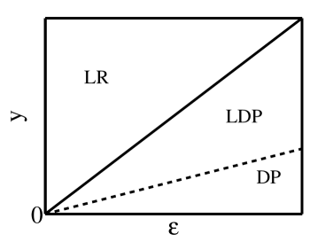
Figure 1: Schematic phase diagram depicting the stable phases of the model with a randomly stirred fluid as the environment. The continuous line which is given by $4y=\epsilon$ is the boundary between the LR and the LDP phases. The dashed line which is given by $\epsilon=2y/3$ is boundary between the LDP and the DP phases.

Let us now compare with Ref. antonov1 where AAPT in contact with a randomly stirred fluid described the NS Eq. with a long-ranged force is considered within a one-loop renormalized perturbation theory like above. Our results for the scaling exponents and the phase diagram are same as that in Ref. antonov1 . The differences between Ref. antonov1 and ours lie essentially in the details: Our choice for the coupling constants is slightly different from Ref. antonov1 . Let us reconsider our choice for the effective coupling constants as used in the calculations above: The expressions of the $Z$-factors in (20) as well as $Z_{\theta}$ reveal that $u,\,w$ and $\tilde{w}=\lambda^{2}D_{1}/[D_{\nu}D(D_{\nu}+D)]$ appear as the bare (dimensionless) expansion parameters in which the one-loop perturbative expansions are linear; but these are not linear in $\theta$. Finally, our assumption of (bare) $\theta\ll 1$ allows us to write $Z_{\tilde{w}}$ as a linear function of $\tilde{w}$ as well. In contrast to us, Ref. antonov1 worked with $u,w$ and $e$ ($\theta$ in our notation) as coupling constants in which the perturbative expansions are made. Our main operational motivation of expanding in terms of $u,w$ and $\tilde{w}$ is that $u$ and $\tilde{w}$ (or rather their renormalized counterparts $u_{R}$ and $\tilde{w}_{R}$) directly describe the relative importance of the original DP nonlinearity vis-a-vis the advective nonlinearity. Hence, the plausibility of four possible phases described by ($u_{R}=0=\tilde{w}_{R}$), ($u_{R}\neq 0,\tilde{w}_{R}=0$), ($u_{R}\neq 0,\,\tilde{w}_{R}\neq 0$) and ($u_{R}=0,\,\tilde{w}_{R}\neq 0$) becomes immediately clear, a fact borne out by the detailed calculations described above. Nevertheless, there is no real contradiction between this work and Ref. antonov1 as is evident by the same values for the scaling exponents and same phase diagram.

II.3 Extinction transition in an environment of a fluctuating surface

Consider next birth/death process of an agent taking place on a fluctuating surface: We thus now discuss the situation, where the dynamics of a population density field $\phi$ near its extinction transition is assumed to be in contact with a fluctuating/growing surface without any overhangs, represented by a scalar height field $h(x,t)$, measured from an arbitrary substrate, which satisfies the nonlinear KPZ equation kpzref or the linear EW barabasi-book equation of motion.

II.3.1 Edward-Wilkinson surface growth equation

The EW Eq.barabasi-book is the simplest equation that describes a growing surface by a single valued height field $h({\bf x},t)$:

$$\frac{\partial h}{\partial t}=D_{h}\nabla^{2}h+\psi.$$ (40)

We consider the noise $\psi$ is zero-mean, Gaussian distributed with a variance given by Eq. (41). We are concerned here with the effects of long ranges noises. The variance of the noise $\psi({\bf k},t)$ in the Fourier space is chosen to be

$$\langle\psi({\bf q},t)\psi(-{\bf q},0)\rangle=2D_{1}q^{2-y-d}\delta(t),$$ (41)

where $D_{1}$ is a constant setting the amplitude and the parameter $y>0$. EW Eq. (40) is not invariant under the Galilean invariance. Eq. (40), owing to its linearity, can be solved exactly. In particular, its dynamic exponent $z_{h}=2$, regardless of the value of $y$.

II.3.2 Kardar-Parisi-Zhang equation

The KPZ equation kpzref is a nonlinear generalization of the EW Eq. above and is given by

$$\frac{\partial h}{\partial t}+\frac{\lambda_{1}}{2}(\nabla h)^{2}=D_{h}\nabla^{2}h+\psi,$$ (42)

where $h$ is the height field which gives the height of the growing surface from a reference plane, $\lambda_{1}$ a coupling constant, $D_{h}$ is a diffusion constant, and $\psi$ is the external noise. Evidently, the EW Eq. (40) can be obtained from the KPZ Eq. (42) by setting $\lambda_{1}=0$. Due to the Galilean (tilt) invariance (see below) of the KPZ equation the coupling constant $\lambda_{1}$ does not renormalize. Analogous to the NS Eq. (6) one defines dynamic exponent $z_{h}$ and the roughness exponent $\chi_{h}$ for characterization of the correlations of the fluctuations of $h$: One writes

$$\langle h({\bf x},t)h(0,0)\rangle\sim|x|^{2\chi_{h}}f_{h}(x^{z_{E}}/t),$$ (43)

where $f_{h}$ is a scaling functions. Nonrenormalization of $\lambda_{1}$ yields an exact relation $\chi_{h}+z_{E}=2$. When $\psi$ is a zero-mean Gaussian distributed white noise, the KPZ equation describes a smooth to rough phase transition at $d>2$ natterman . We will however be concerned here with the situation when the KPZ equation (42) is driven by a long range noise, same as (41). Stochastic dynamics of the KPZ equation driven by a long ranged correlated noise has already been studied extensively in Ref. medina by using DRG methods. Such applications suffer from several technical complications which are similar in nature to those for the NS Eq. (6) with a long-ranged noise. Nevertheless, one-loop DRG calculations have been successful is obtaining the scaling exponents. As for the randomly stirred fluid model, the only quantity that renormalizes here is the diffusion coefficient $D_{h}$. Explicit one-loop RG calculation yield $z_{E}=2-y/3$ medina ; freylong , an expression which is identical for a given $y$ to that in the randomly stirred NS Eq. (6).

II.3.3 Extinction transition in contact with an Edward-Wilkinson fluctuating surface

Let us now assume that the percolating agent $\phi$ is coupled to a fluctuating surface described by the EW equation (40). Thus an EW surface now forms the environment of the percolating process. On general symmetry ground the time evolution of the density field $\phi$ may be written as

$$\frac{\partial\phi}{\partial t}+\lambda_{2}(\nabla h)\cdot(\nabla\phi)+\lambda_{3}\phi\nabla^{2}h=D\nabla^{2}\phi+\lambda_{g}\phi-\lambda_{d}\phi^{2}+\sqrt{\phi}\zeta,$$ (44)

where $\lambda_{2}$ and $\lambda_{3}$ are coupling constants. Equation (44) may be written as

$$\frac{\partial\phi}{\partial t}+\hat{\lambda}(\nabla h)\cdot(\nabla\phi)+\lambda_{3}\nabla\cdot(\phi\nabla h)=D\nabla^{2}\phi+\lambda_{g}\phi-\lambda_{d}\phi^{2}+\sqrt{\phi}\zeta,$$ (45)

where $\hat{\lambda}=\lambda_{2}-\lambda_{3}$. The $\lambda_{3}$-term in Eq. (45), being a gradient term, is irrelevant in the long wavelength hydrodynamic limit (which is our region of interest here). Thus the effective equation for $\phi$ that we are going to work with is

$$\frac{\partial\phi}{\partial t}+\hat{\lambda}(\nabla h)\cdot(\nabla\phi)=D\nabla^{2}\phi+\lambda_{g}\phi-\lambda_{d}\phi^{2}+\sqrt{\phi}\zeta.$$ (46)

Just as in the previous case of a randomly stirred fluid environment, on grounds of general arguments we expect to find four different phases characterized by four different fixed points - Gaussian, DP, LDP and LR. The first two correspond to weak dynamic scaling where as the last two should display strong dynamic scaling. The EW Eq. (40) being linear the corresponding dynamics has a dynamic exponent $z_{E}=2$. Thus, strong dynamic scaling for the density field $\phi$ implies it will display dynamic scaling characterized by an exponent $z_{\phi}=2$. Although this corresponds to its value of the linearized theory [see the mean-field exponents given by Eq. (4)], it does not really correspond to an AAPT characterized by the mean-field exponents, since all the other critical exponents (e.g., $\eta,\nu$ etc) differ from their mean-field values. Our calculations below confirms this picture.

Using Eqs. (46) and (40) we can write down the generating functional for the model given by ${\mathcal{Z}}_{EW}=\int DhD\hat{h}D\phi D\hat{\phi}\exp[S_{EW}]$, where $S_{EW}$ is the action of the model. Function $\hat{h}$ and $\hat{\phi}$ are the conjugate auxiliary fields which appear due to the averaging over the noise distributions. Now to simplify the action and the calculations subsequently we rescale the fields as $\hat{\phi}\rightarrow i\alpha\hat{\phi}$, $\hat{h}\rightarrow i\hat{h}$ and $\phi\rightarrow\beta\phi$ with $\alpha\beta=1$. The parameters are then rescaled as $D_{1}\alpha^{2}\beta={Dg_{2}\over 2}$, $\lambda_{d}\alpha\beta^{2}={Dg_{1}\over 2}$ and $\lambda_{g}=\tau D$. This modified action can be written as

$$S_{EW}(h,\hat{h},\phi,\hat{\phi}) = D_{2}\int\frac{d^{d}k}{(2\pi)^{d}}\int dt\hat{h}\hat{h}k^{2-y-d}-\int\frac{d^{d}k}{(2\pi)^{d}}\hat{h}\{\partial_{t}h+D_{h}q^{2}h\}-\int\frac{d^{d}k}{(2\pi)^{d}}\hat{\phi}\{\partial_{t}\phi-\hat{\lambda}\sum_{\bf q}h({\bf q})\phi({\bf k-q}){\bf q}\cdot{\bf(k-q)}$$ (47)

$$+ Dk^{2}\phi-\tau D\phi+{D\over 2}\sum_{\bf q}[g_{1}\phi({\bf q})\phi({\bf k-q})-g_{2}\hat{\phi}({\bf q})\phi({\bf k-q})]\}.$$

Note that action (47) is not invariant under the rapidity transformation, similar to action (13) . As before, we are required to identify all the primitive divergent one-loop vertex functions. The vertex generating functional $\Gamma_{EW}$ is defined in the standard way as $\log{\mathcal{Z}}_{EW}$. The EW equation (40) being linear, there are no corrections to the vertex functions $\frac{\delta^{2}\Gamma_{EW}}{\delta h\delta\hat{h}}$ and $\frac{\delta^{2}\Gamma_{EW}}{\delta\hat{h}\delta\hat{h}}$, where $\Gamma_{EW}$ is the Legendre transformation of $\log Z_{EW}$. However, there are now non-zero one-loop fluctuation corrections to $\hat{\lambda}$. Thus, the vertex functions that are to be renormalized in order to render the action (47) finite are (i) $\frac{\delta^{2}S_{EW}}{\delta\phi\delta\hat{\phi}}$, (ii) $\frac{\delta^{3}S_{EW}}{\delta\hat{\phi}\delta\phi\delta\phi}$, and (iii) $\frac{\delta^{3}S_{EW}}{\delta\hat{\phi}\delta\hat{\phi}\delta\phi}$. The (bare) coupling constants for the present problem are $u_{R}=g_{1}g_{2},\,w=\frac{\lambda^{2}}{D^{3}}$. In addition, dimensionless Schimdt number $\theta=D_{h}/D$ appears as a control parameter. Assuming renormalizability, we introduce renormalization $Z$-factors for each of the primitive divergent vertex functions: (i) $\frac{\delta^{2}\Gamma_{EW}}{\delta\phi\delta\hat{\phi}}$, (ii) $\frac{\delta^{3}\Gamma_{EW}}{\delta\phi\delta\phi\delta\hat{\phi}}$, (iii) $\frac{\delta^{3}\Gamma_{EW}}{\delta\hat{\phi}\delta\hat{\phi}\delta\phi}$, and (iv) $\frac{\delta^{3}\Gamma_{EW}}{\delta h\delta\hat{\phi}\delta\phi}$. We use a minimal subtraction scheme, in which diverging parts of the associated one-loop fluctuation correction integrals are evaluated in inverse power series of $\epsilon=4-d$ and $y$.

The renormalized fields and the parameters are related to the corresponding bare quantities through the relation

$$\phi=Z^{R}\phi^{R}\,\,,\,\,\hat{\phi}=\hat{Z}^{R}\hat{\phi}^{R},\,\,\,\tau=Z_{\tau}\tau^{R}\,\,,\,\,D=Z_{D}D^{R}\,\,,\,\,g_{1}=Z_{g_{1}}g_{1}^{R}\,\,,\,\,g_{2}=Z_{g_{2}}g_{2}^{R}\,\,\,\mbox{and}\,\,\,\hat{\lambda}=Z_{\hat{\lambda}}\hat{\lambda^{R}}.$$ (48)

We evaluate the $Z$-factors of the renormalized action in terms of the coupling constants $u=g_{1}g_{2}$ and $\hat{w}=D_{1}\hat{\lambda}^{2}/D^{3}$ and rescale these coupling constants with a factor of $1/16\pi^{2}$ as we have done before in Section II.2. Writing Schmidt number $\theta={D_{h}\over D}$, the $Z$-factors are written as

$$Z = \hat{Z}=1+\frac{u}{8}\frac{\mu^{-\epsilon}}{\epsilon},$$ (49)

$$Z_{\tau} = 1-{3u\over 8\epsilon}\mu^{-\epsilon}-{\hat{w}(1-\theta)\over 2\theta(1+\theta)^{2}y}\mu^{-y},$$ (50)

$$Z_{D} = 1-{u\over 8\epsilon}\mu^{-\epsilon}+{\hat{w}(1-\theta)\over 2\theta(1+\theta)^{2}y}\mu^{-y},$$ (51)

$$Z_{u} = 1+{3u\over 2\epsilon}\mu^{-\epsilon}-{\hat{w}(1-\theta)\over\theta(1+\theta)^{2}y}\mu^{-y}-{2\hat{w}\over\theta(1+\theta)y}\mu^{-y},$$ (52)

$$Z_{\hat{\lambda}} = 1+{u\over 8\epsilon}\mu^{-\epsilon}+{\hat{w}\over 2\theta(1+\theta)^{2}y}\mu^{-y}.$$ (53)

The $Z$-factor $Z_{\theta}$ can be easily calculated from Eq. (51) as there is no renormalization for $D_{h}$:

$$Z_{\theta}=Z_{D}^{-1}=1+{u\over 8\epsilon}\mu^{-\epsilon}-{\hat{w}(1-\theta)\over 2\theta(1+\theta)^{2}y}\mu^{-y}.$$ (54)

The renormalized coupling constants are defined as

$$u^{R}=uZ_{u}^{-1}\mu^{-\epsilon}\,\,,\,\,\hat{w}^{R}=\hat{w}Z_{\hat{w}}^{-1}\mu^{-y},\,\,,\,\,\theta^{R}=\theta Z_{\theta}^{-1},\,\,\,w^{R}=wZ_{w}^{-1}\mu^{-y}.$$ (55)

The critical exponents are derived from these flow functions at the fixed points of the model which are evaluated easily from the beta functions

$$\beta_{u}=\mu{\partial\over\partial\mu}u^{R}\,\,,\,\,\beta_{\hat{w}}=\mu{\partial\over\partial\mu}w^{R}\,\,,\,\,\beta_{\theta}=\mu{\partial\over\partial\mu}\theta^{R}.$$ (56)

At the RG fixed point then we have

$$\beta_{\hat{w}}=w^{R}\left(-y+{5u^{R}\over 8}+{w^{R}\over\theta^{R}(1+\theta^{R})^{2}}-{3\hat{w}^{R}(1-\theta^{R})\over 2\theta^{R}(1+\theta^{R})^{2}}\right),$$

$$\beta_{u}=u^{R}\left(-\epsilon+{3\over 2}u^{R}-{\hat{w}^{R}(1-\theta^{R})\over\theta^{R}(1+\theta^{R})^{2}}-{2\hat{w}^{R}\over\theta^{R}(1+\theta^{R})}\right),$$

$$\beta_{\theta}=\theta^{R}\left({1\over 8}u^{R}-{\hat{w}^{R}(1-\theta^{R})\over 2\theta^{R}(1+\theta^{R})^{2}}\right).$$ (57)

Fixed points of the model can be obtained from $\beta_{u},\,\beta_{\hat{w}}$ and $\beta_{\theta}$ by setting them all to zero. Note that the value of $\theta_{R}$ at the fixed points cannot exceed $1$. In fact the range is $1\leq\theta_{R}\leq 0$. The different fixed point solutions are as follows:

• Gaussian fixed point: $u^{R}=0=\hat{w}^{R}$, $\theta^{R}=\theta$ (bare value of the Schmidt number which is any finite positive number).

• DP fixed point:$u^{R}=2\epsilon/3$, $\hat{w}^{R}=0$, $\theta^{R}=0$.

• Long range fixed point (LR): $u^{R}=0,\hat{w}^{R}=4y,\theta^{R}=1$.

• Long range DP fixed point (LDP): $u^{R}\neq 0,\,\hat{w}^{R}\neq 0,\,\theta^{R}<1$. We discuss this fixed point in details below.

At the LDP fixed point values of $u^{R}$, $\hat{w}^{R}$ and $\theta^{R}$ satisfy the coupled equations

$$\frac{3}{2}u^{R}-2\frac{\hat{w}^{R}}{\theta^{R}(1+\theta^{R})}-\hat{w}^{R}\frac{1-\theta^{R}}{\theta^{R}(1+\theta^{R})^{2}} = \epsilon,$$ (58)

$$\frac{u^{R}}{2}+2\frac{\hat{w}^{R}}{\theta^{R}(1+\theta^{R})^{2}}-\frac{\hat{w}^{R}(1-\theta^{R})}{\theta^{R}(1+\theta^{R})^{2}} = y,$$ (59)

$$\frac{u^{R}}{4}-\hat{w}^{R}\frac{1-\theta^{R}}{\theta^{R}(1+\theta^{R})^{2}} = =0.$$ (60)

The solutions are given by

$$u^{R}=4(2y+\epsilon)/9,\;\;\;\hat{w}^{R}=\frac{2}{9}\frac{(5y-2\epsilon)^{2}}{y-\epsilon},\;\;\;\theta^{R}=3\frac{y-\epsilon}{7y-\epsilon}.$$ (61)

Fixed point values (61) formally define the LDP fixed point. Positivity of $\theta_{R}$ demands that solutions (61) are meaningful only if either $y>\epsilon$ or $7y<\epsilon$, such that the ratio $(y-\epsilon)/(7y-\epsilon)$ is positive. However, when $y<\epsilon$ and $7y>\epsilon$, $\theta$ is negative and hence solutions (61) are not physical. With the knowledge of the fixed point values of the coupling constants, one can now easily write down the corresponding scaling exponents: At the DP fixed point $({2\epsilon\over 3},0,0)$, the anomalous dimension $\eta_{\phi}=\eta_{\hat{\phi}}$, the dynamic exponent $z$ and the correlation length exponent $\nu$ are given by

$$\eta_{\phi}=\eta_{\hat{\phi}}={\epsilon\over 12}\,\,,\,\,z_{\phi}=2-{\epsilon\over 12}\,\,,\,\,{1\over\nu}=2+{\epsilon\over 4}.$$ (62)

At the LR fixed point $(0,4y,1)$, the same critical exponents turn out to be

$$\eta_{\phi}=\eta_{\hat{\phi}}=0\,\,,\,\,z_{\phi}=2\,\,,\,\,{1\over\nu}=2.$$ (63)

Lastly, at the LDP fixed point we find

$$\eta_{\phi} = \eta_{\hat{\phi}}=\frac{1}{18}(2y+\epsilon),$$ (64)

$$\nu^{-1} = 2-\gamma_{\tau}=2+\frac{1}{9}(2y+\epsilon),$$ (65)

$$z_{\phi} = 2.$$ (66)

Thus, clearly both the LDP and LR fixed points correspond to strong dynamic scaling as the dynamic exponent of the density field $z_{\phi}=2=z_{E}$, the dynamic exponent of the EW surface. Although this is identical to the mean-field value of $z_{\phi}$, the scaling behaviors described by the LR and LDP fixed points do not correspond to mean-field scaling as can be easily seen from the values of the other exponents.

Finally let us briefly consider linear stability analysis of the different phases, which can be performed in a standard way analogous to the previous case of randomly stirred fluid environment. We find, unsurprisingly, that the Gaussian FP is always unstable for any $\epsilon>0$ and $y>0$. The DP FP is stable for $\epsilon>3y$. In contrast the LR FP is always unstable, unlike the case when the environment is modeled by a randomly stirred fluid. We do not discuss the stability of the LDP FP due to the associated algebraic complications. However, the determinant of the stability matrix at the LDP FP vanish for $y=\epsilon$, suggesting borderline between stability and instability. Incidentally, the line $y=\epsilon$ demarcates the region of existence of the LDP FP. Further, since the LDP FP does not exist for $y<\epsilon<7y$ and DP FP is unstable for $\epsilon<3y$, there is no physically meaningful solution in the region $y<\epsilon<3y$, a situation that does not arise when the environment is a randomly stirred fluid. Fig. (2) below shows the stable phases of the model with a fluctuating EW surface as the environment.

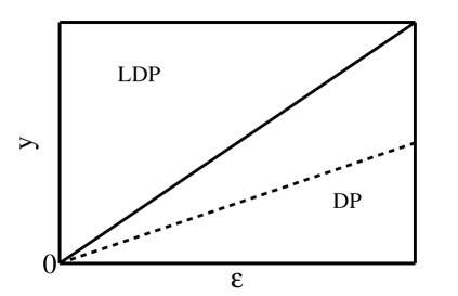
Figure 2: Schematic phase diagram depicting the stable phases of the model with an EW surface as the environment. The continuous line is given by $y=\epsilon$ such that the LDP phase exists for $y>\epsilon$. The dashed straight line is given by $y=\epsilon/3$; the usual DP phase exists for $\epsilon>3y$. There is no physically meaningful phase in the region between the lines $y=\epsilon$ and $y=\epsilon/3$.

II.3.4 AAPT in contact with a fluctuating KPZ surface

We now briefly consider how a fluctuating KPZ surface may affect the universal properties of extinction transition of a population density $\phi$ near its threshold. Due to associated algebraic complications our studies in this section are less extensive. Nevertheless we are still able to obtain physically interesting results consistent with the results obtained elsewhere in this paper. Field $\phi$ follows Eq. (46), as in the case when the environment is modeled by a growing EW surface. However, unlike the case of the environment modeled by the EW Eq. (40) for the specific choice $\lambda_{1}=\lambda_{2}$, Eqs. (42) and (44) are invariant under the tilt transformation:

$$h\rightarrow h+{\mathbf{\varepsilon}}\cdot{\bf x},\,\,\phi\rightarrow\phi,\,\,\,{\bf x}\rightarrow{\bf x}-\lambda_{1}{\mathbf{\varepsilon}}t.$$ (67)

As previously, Eq. (44) reduces to Eq. (46) after discarding total derivative terms in the long wavelength limit. Function $\xi$ is a zero mean Gaussian white noise with a variance (2). As before, the multiplicative nature of noise ensures that the absorbing state $\phi=0$ is a solution of Eq. (46). Similar to the case of a randomly stirred fluid environment, on general physical ground we expect four different DRG fixed points to exist, corresponding to four distinct phases: (i) Gaussian, (ii) DP, (iii) LDP, (iv) LR. The Gaussian FP is expected to be always unstable. The DP FP corresponds to weak dynamic scaling, where as phases corresponding to the LDP and LR FPs should display strong dynamic scaling.

For performing DRG calculations, we use a path integral formulation in terms of the Janssen-De Dominicis generating functional corresponding to the KPZ Eq. (42) together with the Gaussian long range noise with a variance (41) for correlation functions as before. Rescaling as for the case with a fluctuating EW surface as the environment, the action functional now reads [after dropping total spatial derivative terms, see the discussions preceding (47)]

$$S_{KPZ}(h,\hat{h},\phi,\hat{\phi}) = 2D_{2}\int\frac{d^{d}k}{(2\pi)^{d}}\int dt\hat{h}\hat{h}k^{2-y-d}-\int\frac{d^{d}k}{(2\pi)^{d}}\int dt\hat{h}\{\partial_{t}h-{\lambda_{1}\over 2}\sum_{\bf q}{\bf q\cdot(k-q)}h({\bf q})h({\bf k-q})+D_{h}k^{2}h\}$$ (68)

$$-\int\frac{d^{d}q}{(2\pi)^{d}}\int dt\hat{\phi}[\partial_{t}\phi-\hat{\lambda}\sum_{{\bf q}}{\bf q\cdot(k-q)}h({\bf q})\phi({\bf k-q})+Dk^{2}\phi-D\tau\phi$$

$$+ {D\over 2}\sum_{\bf q}[g_{1}\phi({\bf q})\phi({\bf k-q})-g_{2}\hat{\phi}({\bf q})\phi({\bf k-q})]].$$

Here again $\hat{h}$ and $\hat{\phi}$ are auxiliary (conjugate) fields. Like (13), action (68) is no longer invariant under the rapidity symmetry. Consequently, nonlinear coefficients $g_{1}$ and $g_{2}$ in general are unequal. As for the usual DP problem, the system exhibits a continuous phase transition from active to absorbing states as (renormalized or effective) $\tau\rightarrow 0$. The associated universal scaling exponents are formally defined as in (3) above. At the mean-field level, the model Eqs. (42) and (46) yield the same values for the scaling exponents as in Sec. II.1. Just like the model in Sec. II.2, nonlinear couplings $\lambda$ and $Dg_{1},\,Dg_{2}$, together with the expected large fluctuations near the critical point and multiplicative nature of the noise with the long-ranged variance (7) substantially alter the mean-field values of the exponents, a fact which we confirm below by our one-loop DRG calculation. Although in general $g_{1}\neq g_{2}$, it is only the product $g_{1}g_{2}$ that appears in the perturbative expansion.

The structure of the perturbation theory and its renormalization is very similar to those in Sec. II.2 above. Due to the long ranged nature of the noise variance (41) there is no renormalization of $D_{1}$. As in the previous case in Sec. II.3.3, the role of the coupling constants in the ordinary perturbation theory in the present model is played by $u=g_{1}g_{2},\;\;\;w=\frac{1}{D_{h}^{3}},\,\,\,\hat{w}=\frac{\hat{\lambda}^{2}}{D^{3}}$.We again consider $\epsilon>0,\,y>0$, for which non-trivial critical exponents will ensue. The vertex generating functional $\Gamma_{KPZ}$ is defined as the Legendre transformation of $\log{\mathcal{Z}}_{KPZ}$. Galilean invariance of the action functional (68) ensures that the three-point vertex function $\frac{\delta^{3}\Gamma_{KPZ}}{\delta\hat{h}\delta h\delta h}$ does not renormalize in the hydrodynamic limit. The vertex functions, which must be renormalized in order to render the present model renormalized, are (i) $\frac{\delta^{2}S_{KPZ}}{\delta h\delta\hat{h}}$, (ii) $\frac{\delta^{2}S_{KPZ}}{\delta\phi\delta\hat{\phi}}$, (iii) $\frac{\delta^{3}S_{KPZ}}{\delta\hat{\phi}\delta\phi\delta\phi}$, (iv) $\frac{\delta^{3}S_{KPZ}}{\delta\hat{\phi}\delta\hat{\phi}\delta\phi}$, and $\frac{\delta^{3}S_{KPZ}}{\delta\hat{\phi}\delta\phi\delta h}$. Using standard methods as described in the previous Sections we in details perform one-loop multiplicative renormalization by introduction of the renormalization $Z$-factors, which render the theory UV finite. We use dimensional regularization together with minimal expansion to enumerate the renormalization $Z$-factors. From the renormalization $Z$-factors, one may then derive the RG flow equation in the usual way. Finally, the scaling behavior of the correlation or vertex functions may be extracted by finding their dependence on $\mu$ by using the RG equation derived below. The renormallization $Z$-factors for the fields and the parameters are defined as

$$\phi=Z\phi^{R}\,\,,\,\,\hat{\phi}=\hat{Z}\hat{\phi}^{R},\,\,\,\tau=Z_{\tau}\tau^{R}\,\,,\,\,D=Z_{D}D^{R}\,\,,\,\,g_{1}=Z_{g_{1}}g_{1}^{R},\,\,,\,\,g_{2}=Z_{g_{2}}g_{2}^{R},\,\,\hat{\lambda}=Z_{\hat{\lambda}}\hat{\lambda}^{R},\,\,\mbox{and}\,\,D_{h}=Z_{D_{h}}D_{h}^{R}.$$ (69)

We evaluate the $Z$-factors of the renormalized action in terms of the coupling constants $u=g_{1}g_{2}$ and $w=D_{2}/D_{h}^{3}$ and rescale these coupling constants with a factor of $1/16\pi^{2}$ as we have done before in Section II.2.2. The different $Z$-factors are

$$Z = \hat{Z}=1+\frac{u}{8}\frac{\mu^{-\epsilon}}{\epsilon},$$ (70)

$$Z_{\tau} = 1+{3u\over 8\epsilon}\mu^{-\epsilon}+{\hat{w}\over 2\theta(1+\theta)}\frac{1-\theta}{1+\theta}\frac{\mu^{-y}}{y},$$ (71)

$$Z_{D} = 1-{u\over 8\epsilon}\mu^{-\epsilon}-{\hat{w}\over{2\theta(1+\theta)}}\frac{1-\theta}{1+\theta}\frac{\mu^{-y}}{y},$$ (72)

$$Z_{u} = 1+{3u\over 2\epsilon}\mu^{-\epsilon}-{2\hat{w}\over{\theta(1+\theta)}}\frac{\mu^{-y}}{y}-\frac{3}{2}\frac{\hat{w}(\theta-1)}{2\theta(1+\theta)^{2}}\frac{\mu^{-y}{y}}{,}$$ (73)

$$Z_{\hat{\lambda}} = 1+\frac{u}{8}\frac{\mu^{-\epsilon}}{+}\frac{\hat{w}}{\theta(1+\theta)^{2}}\frac{\mu^{-y}}{y}-\sqrt{w}\sqrt{\hat{w}}\frac{1+3\theta}{\sqrt{\theta}(1+\theta)^{2}},$$ (74)

$$Z_{\hat{w}} = 1+\frac{5u}{8}\frac{\mu^{-\epsilon}}{\epsilon}+\frac{2\hat{w}}{\theta(1+\theta)^{2}}\frac{\mu^{-y}}{y}+\frac{3\hat{w}}{2\theta(1+\theta)}\frac{\theta-1}{\theta+1}\frac{\mu^{-y}}{y}-2\sqrt{w}\sqrt{\hat{w}}\frac{1+3\theta}{\sqrt{\theta}(1+\theta)^{2}},$$ (75)

$$Z_{D_{h}} = 1-{wb\over y}\mu^{-y},$$ (76)

where $b=y/4d$medina .

The renormalized coupling constants are written as

$$u^{R}=uZ_{u}^{-1}\mu^{-\epsilon}\,\,,\,\,w^{R}=wZ_{w}^{-1}\mu^{-y}\,\,,\,\,\hat{w}^{R}=\hat{w}Z_{\tilde{w}}^{-1}\mu^{-y},\,\,\,\theta^{R}=\theta Z_{\theta}^{-1}.$$ (77)

The critical exponents are obtained from the Wilson’s flow functions at the fixed points of the model which are evaluated easily from the zeros of the beta functions

$$\beta_{u}=\mu{\partial\over\partial\mu}u^{R}\,\,,\,\,\beta_{w}=\mu{\partial\over\partial\mu}w^{R}\,\,,\,\,\beta_{\tilde{w}}=\mu{\partial\over\partial\mu}\tilde{w}^{R},\,\,\,\beta_{\theta}=\mu\frac{\partial}{\partial\mu}\theta^{R}.$$ (78)

At the RG fixed point then we have

$$\beta_{\hat{w}} = \hat{w}^{R}\left[-y+\frac{5}{8}u^{R}+\frac{2\hat{w}^{R}}{\theta^{R}(1+\theta^{R})^{2}}-\frac{3\hat{w}^{R}}{2\theta^{R}(1+\theta^{R})}\frac{1-\theta^{R}}{1+\theta^{R}}-2\sqrt{w^{R}}\sqrt{\hat{w}^{R}}\frac{1+3\theta^{R}}{\sqrt{\theta^{R}}(1+\theta^{R})^{2}}\right],$$

$$\beta_{u} = u^{R}\left[-\epsilon+{3\over 2}u^{R}-\frac{2\tilde{w}^{R}}{\theta^{R}(1+\theta^{R})}+\frac{\hat{w}^{R}}{\theta^{R}(1+\theta^{R})}\frac{\theta^{R}-1}{\theta^{R}+1}\right],$$

$$\beta_{{w}} = {w}^{R}\left(-y+3bw^{R}\right),$$

$$\beta_{\theta} = \theta^{R}\left[\frac{u^{R}}{8}-\frac{\hat{w}^{R}}{2\theta^{R}(1+\theta^{R})}\frac{1-\theta^{R}}{1+\theta^{R}}-bw^{R}\right].$$ (79)

It is clear that $w^{R}=y/3b$ is the only stable fixed point solution for $w^{R}$. The other solution $w^{R}=0$ is unstable always and we ignore it from our discussions below. While we find the FPs and the corresponding scaling exponents below, we do not discuss their linear stability. Although the latter can in principle be done just as we do for the other models, it is algebraically much more complicated due to the structure of the fixed point equations. As before, we expect four different fixed points to exist, similar to the previous cases. We also expect weak and strong dynamic scaling in different situations. We find

• $\,\,u^{R}=0,\hat{w}^{R}=0\,\,\,\mbox{(Gaussian fixed point)}$. The corresponding scaling exponents are those of the linearized system.
  

• $\,\,u^{R}={2\over 3}\epsilon,\hat{w}^{R}=0\,\,\,\mbox{DP fixed point}$. The exponents are given by those of the DP universality class.
  

• $\,\,u^{R}=0;\hat{w}^{R}\;\;{\rm and}\;\;\theta^{R}$ may be solved from the coupled nonlinear equations

  $$\frac{\hat{w}^{R}}{2\theta^{R}(1+\theta^{R})}\frac{1-\theta^{R}}{1+\theta^{R}}=-bw^{R}=y/3,$$ (80)

  $$\frac{2\hat{w}^{R}}{\theta^{R}(1+\theta^{R})^{2}}-\frac{3\hat{w}^{R}}{2\theta^{R}(1+\theta^{R})}\frac{1-\theta^{R}}{1+\theta^{R}}-2\sqrt{w^{R}}\sqrt{\hat{w}^{R}}\frac{1+3\theta^{R}}{\sqrt{\theta}^{R}(1+\theta^{R})^{2}}=y.$$ (81)

  Explicit solutions of the above equations are a difficult task, owing to their highly nonlinear nature. However, without their explicit solutions, one may already obtain the following information: (i) Since $\hat{w}^{R}>0$, one has $\theta^{R}>1$, thus $D>D_{h}$, (ii) Dynamic exponent $z_{\phi}=2-\gamma^{*}_{D}=2-\frac{\hat{w}^{R}}{2\theta^{R}(1+\theta^{R})}\frac{1-\theta^{R}}{1+\theta^{R}}=2-y/3=z_{E}$ and hence strong dynamic scaling, (iii) correlation length exponent $\nu$ is given by $\nu^{-1}=2-\gamma_{\tau}^{*}=2+y/3$, and (iv) the anomalous dimension $\eta_{\phi}^{*}=\eta_{\hat{\phi}}^{*}=u^{R}/8=0$ at the LR FP.

• LDP fixed point: $u^{R}\neq 0$. Actual enumeration of the fixed point values of the coupling constants are very difficult due to the complicated nonlinear structures of the underlying equations, and will not be discussed here. Using, however, the approximation $\theta^{R}\gg 1$, we obtain $u^{R}=4(\epsilon+2y/3)/7$. Fixed point values $\theta^{R}$ and $\hat{w}^{R}$ are to be obtained from the coupled nonlinear equations

  $$\sqrt{\hat{w}^{R}}=\theta^{R}\sqrt{\frac{4y-\epsilon}{21}},$$ (82)

  $$\frac{\epsilon+2y/3}{7}+\frac{2\hat{w}^{R}}{\theta^{R}(1+\theta^{R})^{2}}-\sqrt{w^{R}}\sqrt{\hat{w}^{R}}\frac{1+3\theta^{R}}{\sqrt{\theta^{R}}(1+\theta^{R})^{2}}=0.$$ (83)

  With $w^{R}=y/3b$ the above two equations may in principle be solved and solutions be obtained with the overall approximation of large $\theta^{R}$. We do not solve these here explicitly. Nevertheless, we can already extract useful information without having to solve for the coupling constants explicitly. We find: (i) dynamic exponent $z_{\phi}=2-\gamma^{*}_{D}=2-\frac{u^{R}}{8}-\frac{\hat{w}^{R}}{2\theta^{R}(1+\theta^{R})}\frac{1-\theta^{R}}{1+\theta^{R}}=2-y/3=z_{E}$ and hence strong dynamic scaling, (ii) correlation length exponent $\nu$ is given by $\nu^{-1}=2-\gamma_{\tau}^{*}=2+3u^{R}/8-\hat{w}^{R}(1-\theta^{R})/[2\theta^{R}(1+\theta^{R})^{2}]=2+u^{R}/4+bw^{R}=2+(\epsilon+2y/3)/7+y/3$, (iii) anomalous dimension $\eta_{\phi}^{*}=\eta_{\hat{\phi}}^{*}=u^{R}/8=(\epsilon+2y/3)/14$, and (iv) by using positivity of $\theta^{R}$ and $\hat{\omega}^{R}$, $4y>\epsilon$ from Eq. (82) for physically meaningful solution.

Thus, with a KPZ surface as a fluctuating environment for an extinction transition that, otherwise (i.e., with a uniform environment) belongs to the DP universality class, the broad emerging picture is similar to the other two models of fluctuating environment considered here before. One generally finds both weak and strong dynamic scaling in different regions of the phase space spanned by $\epsilon$ and $y$. The details, including the values of the scaling exponents, may of course depend upon the actual model of the fluctuating environment. Lastly, some technical comments regarding alternatives to the DRG procedure here is in order: As we commented before, the one-loop DRG procedure for the KPZ Eq. (42) with long ranged noise suffer well-known technical problems. As an alternative to it, self-consistent mode coupling method (SCMC) scmc and functional renormalization group (FRG) frg have been used to extract large length-scale, long-time physics of the KPZ Eq. with long ranged noise. The SCMC expansion, as illustrated in Ref. scmc , yields results which match with those in Ref. medina at $1d$, where as for $d>1$ the results of Ref. scmc differ substantially from Ref. medina and yields much more physically sensible results in the limit of short ranged noise. Similarly, Ref. frg uses the well-known Cole-Hopf transformation and applies the FRG (up to two-loop) on the resulting partition function to obtain scaling exponents for the KPZ Eq. (42) with long-ranged noises. Their results clearly highlight the short comings of the one-loop DRG procedure. While the qualitative picture that emerges out of our one-loop DRG calculations here are expected to remain on general physical grounds, it will be interesting to calculate the details of the AAPT transition in contact with a KPZ surface by using the SCMC or FRG methods as illustrated in Refs. scmc ; frg . The EW Eq. (40) being linear such technical issues as for the KPZ Eq. do not arise. Nevertheless, investigation of the associated AAPT transition (in contact with an EW surface) by using SCMC or FRG methods would be useful.

III Summary and outlook

This article is a study of how non-trivial fluctuating spatio-temporal dynamics of the environment may affect the usual directed percolation process with constant environment. We have separately considered cases when the environment is a (i) randomly stirred fluid described by the Navier-Stokes equation with a long-ranged force, (ii) a fluctuating surface with long-ranged spatial correlation, described either by the KPZ or the EW equations driven by a long-ranged noise. Our model systems are semi-autonomous, i.e., we ignore feedback due to the percolating field on the environment. The general picture that emerges out of our calculations is that depending upon relative values of $\epsilon=4-d$ and $y$, a parameter that fixes the spatial scaling of variances of the external forces in the NS, EW or KPZ equations, one obtains different universal behavior. However, the details of the ensuing phase diagram in the $\epsilon-y$ plane depend explicitly on the model used to describe the environment (NS, EW or KPZ). On general ground we predict possibilities of four different phases (i) Gaussian, (ii) original DP, (iii) Long-range DP (LDP) and (iv) Long-range (LR). The Gaussian fixed point is generally unstable. The rest are model dependent (i.e., depends upon whether the environment is modeled by the NS, EW or KPZ Eq.). For a randomly stirred environment described by the NS Eq., we find when $\epsilon>4y$, the ensuing universal critical behavior of the AAPT transition is described by the standard DP universality class characterized the DP fixed point with the renormalized coupling constants $u^{R}=2\epsilon/3$, $\tilde{w}^{R}=0$, corresponding to a dynamic exponent $z_{\phi}<z_{E}$, the dynamic exponent of the environment. Thus one obtains weak dynamic scaling, despite the nonlinear coupling between $\phi$ and the environment (here: velocity $\bf v$). In the other regime, i.e., when $\epsilon<4y$, the DP fixed point gets unstable against perturbations due to the environmental fluctuations, and the AAPT is described by a set of critical exponents that depend upon $y$. The corresponding phases are described by either the LDP fixed point $u^{R}=4\epsilon/5-8y/15$ and $\tilde{w}^{R}=8y/15-2\epsilon/15$, or by the LR fixed point $u^{R}=0$ and $\tilde{w}^{R}=4y/9$. In both these regimes $z_{\phi}=z_{E}=2-y/3$, thus describing strong dynamic scaling. We obtain the relevant scaling exponents in all the phases. Agreement of our results for the scaling exponents and the phase diagram with those in Ref. antonov1 shows the general robustness of the perturbation theory, despite our using (slightly) different choices for the coupling constants. It also shows how such choices may be exploited to infer the large length-scale, long-time limit physics of the system in a simple manner. In contrast, when the environment is a fluctuating surface modeled by the EW Eq., the DP phase is linearly stable for $\epsilon>3y$. We further find that the LR phase is not at all stable for any $y>0$. Furthermore, the LDP phase does not exist in the range $y<\epsilon<7y$. Thus, the phase diagram in this case does not have any physically meaningful phase in the range $y<\epsilon<3y$, unlike the NS case where the phase diagram is fully spanned by the stable phases of the system. The LDP phase here corresponds to strong dynamic scaling and the DP phase weak dynamic scaling. We obtain the associated scaling exponents as well. For an environment described by a fluctuating KPZ surface, we again find the existence of four different phases similar to the previous cases. We are able to obtain the scaling exponents in each phase and show that strong dynamic scaling prevails in the LDP and LR phases, as expected. However, due to the algebraically complicated nature of the DRG $\beta$-functions we do not discuss their linear stability here. Validity of our results are limited by the applicability of one-loop approximations which suffer from well-known technical difficulties jkb in systems with long range noises. Thus it is important to verify our results in numerical simulations of the models used here. Further, it is unclear how multiscaling of the velocity field given by the randomly stirred NS model or the height field given by the KPZ equation affect the scaling of the percolating agent $\phi$, or whether $\phi$ itself will display multiscaling for its higher order structure functions. Since the EW equation is a linear equation, it does not show any multiscaling. However still, field $\phi$ may display multiscaling, similar to the passive scalar problem of fluid turbulence, where even if the velocity field is Gaussian distributed (albeit with a long ranged spatial correlation), the passive scalar density exhibits multiscaling passive-scal . We look forward to numerical solutions of the continuum model equations in resolving the outstanding theoretical issues discussed above. In addition, the effects of EW or KPZ fluctuating surfaces on the DP universality may be studied by numerical simulations of lattice-gas type models, which may be constructed by borrowing, e.g., the lattice-gas models used in Ref. lattice to study the dynamics of a passive scalar on fluctuating surfaces. Effects of turbulent flow on the DP universality may in principle be investigated by adopting the experimental set up of Ref. chate and stirring the system with long-ranged external forces, or by observing grwoth/decay of a bacteria colony in a turbulent flow.

Our models and results provide for simple examples of weak dynamic scaling, situations which are not very commonly found. Known examples include the studies in Refs. kardar ; jkb-amit ; das-basu ; uwe1 . Our semi-autonomous models, where effects of the local population on the environment is completely neglected, are certainly a simplification of more realistic situations where such feedback effects should be present in general. A non-zero feedback is known to affect the scaling properties of the NESS in general. For instance, the scaling/multiscaling properties of the magnetic fields in three-dimensional Magnetohydrodynamics ($3d$MHD) are vastly different when the feedback (in the form of Lorentz forces in $3d$MHD) is present from when it is absent (the passive vector limit) mhd . Given this, it would be interesting see how feedback due to $\phi$ may alter the emerging scaling behavior discussed here. When a feedback is present, the overall system is no longer autonomous, but fully coupled. It would be intriguing to see if weak dynamic scaling persists even in the fully coupled case. A truly novel feature of our results is that, in all the three models considered here regardless of stability issues, the LR and the LDP FPs correspond to the same value of the dynamic exponent $z_{\phi}$, but different values for the static scaling exponents $\eta_{\phi},\nu$. This is in contrast with what one finds in equilibrium critical dynamics. For instance, model A and model B (in the nomenclature of Ref. halp ) display different dynamic exponent but the same static critical exponents for the second order phase transition in the $O(N)$ model. Equality of the static critical exponents for different dynamics (i.e., different dynamic exponents) is a requirement of thermal equilibrium. Since our work concerns here models that are driven our of equilibrium, such considerations do not arise. Numerical solutions of the continuum stochastic equations of motion or simulations of equivalent lattice models should be able to verify our results. Beyond immediate theoretical motivation, our work sheds important light for more realistic problems, e.g., population dynamics of a bacteria colony or a biofilm resting over a fluctuating surface or a fluctuating biomembrane. Further, Our results provide important insight for more biologically motivated problems, e.g., population dynamics of a bacteria colony over a fluctuating surface, or in the presence of a macroscopic order, e.g., in a nematic or polar active fluid active .

IV Acknowledgement

One of the authors (AB) wishes to thank the Max-Planck-Society (Germany) and Department of Science and Technology (India) for partial financial support under the Partner Group program (2009).

References

- (1) P. Grassberger and K. Sundermeyer, Phys. Lett. B, 77, 220 (1978).
- (2) P. Grassberger and A. de La Torre, Ann. Phys. (N.Y.), 122, 373 (1979).
- (3) V.N. Gribov, Zh. Eksp. Teor. Fiz., 53, 654 (1967) [Sov. Phys. JETP, 26, 414 (1968)].
- (4) V.N. Gribov and A.A. Migdal, Zh. Eksp. Teor. Fiz., 55, 1498 (1968) [Sov. Phys. JETP, 28, 784 (1969)].
- (5) O. Mollison, J. R. Stat. Soc. B (Methodol.), 39, 283 (1977).
- (6) H.K. Janssen, J. Stat. Phys., 103, 801 (2001).
- (7) P. Grassberger, Z. Phys. B, 47, 365 (1982).
- (8) A comprehensive recent overview over directed percolation is available in H. Hinrichsen, Adv. Phys., 49, 815 (2001); see also M. Henkel, H. Hinrichsen, and S. Lübeck, Non-Equilibrium Phase Transitions, Berlin: Springer (2008).
- (9) For a recent review on the field theory approach to percolation processes, see H.K. Janssen and U.C. Täuber, Ann. Phys. (N.Y.), 315, 147 (2005).
- (10) J. Marro and R. Dickman, Nonequilibrium phase transitions in lattice models (Cambridge University Press, Cambridge, 1999).
- (11) K. A. Takeuchi, M. Kuroda, H. Chaté and M. Sano, Phys. Rev. Lett., 99, 234503 (2007).
- (12) H.K. Janssen, Z. Phys.: Cond. Mat. B, 42, 151 (1981).
- (13) P. Grassberger, in Fractals in Physics, edited by L. Pietronero and E. Tosatti (Elsevier, 1986).
- (14) H. Hinrichsen and M. Howard, Eur. Phys. J. B, 7, 635 (1999).
- (15) H.K. Janssen, K. Oerding, F. van Wijland, and H.J. Hilhorst, Eur. Phys. J. B, 7, 137 (1999).
- (16) H. K. Janssen and P. Stenull, Phys. Rev. E, 78, 061117 (2008).
- (17) N. V. Antonov, V. I. Iglovikov and A. S. Kapustin, J. Phys. A: Math. Theor., 42 135001 (2008).
- (18) N. V. Antonov, A. S. Kapustin and A. V. Malyshev, Theor. Math. Phys. 169, 1470 (2011).
- (19) L. D. Landau and E. M. Lifshitz, Fluid Mechanics, Butterworth-Heinemann (1987).
- (20) D. Forster, D. R. Nelson and M. J. Stephen, Phys. Rev A, 16, 732 (1977).
- (21) V. Yakhot and S. A. Orszag, J. Sci. Comp., 1, 3 (1986).
- (22) In fact, for long range noise with variances (7) the velocity field displays what is known as multiscaling in literature. See, e.g., Ref. rfnse for results and discussions. This is outside the scope of the present discussion.
- (23) J.K. Bhattacharjee, J. Phys. A, 31, L93 (1998).
- (24) D. Ronis, Phys. Rev. A, 36, 3322 (1987).
- (25) R. Bausch, H.K. Janssen and H. Wagner, Z. Phys. B: Cond. Mat., 24, 113 (1976).
- (26) Uwe Täuber, Lect. Notes Phys., 716, 295 (2007).
- (27) Equivalently, the Galilean invariance ensures that the combination of terms enter in the renormalized action only in the form of the Lagrangian derivative , where . Similar considerations apply to .
- (28) A.-L. Barabasi and H. E. Stanley, Fractal Concepts in Surface Growth, Cambridge University Press, Cambridge (1995).
- (29) Lei-Han Tang, T. Nattermann, and B. M. Forrest, Phys. Rev. Lett., 65, 2422 (1990).
- (30) M. Kardar, G. Parisi and Y.-C Zhang, Phys. Rev. Lett., 57, 1810 (1986).
- (31) E. Medina, T. Hwa, M. Kardar and Y.-C Zhang, Phys Rev. A, 39, 3053 (1989).
- (32) H.K. Janssen, U.C. Täuber and E. Frey, Eur. Phys. J. B, 9, 491 (1999).
- (33) E. Katzav and M. Schwartz, Phys. Rev. E, 60, 5677 (1999).
- (34) A. A. Fedorenko, Phys. Rev. B, 77, 094203 (2008).
- (35) G. Falkovich, K. Gawe,dzki, and M. Vergassola, Rev. Mod. Phys., 73, 913 (2001).
- (36) See, e.g., S. Chatterjee and M. Barma, cond-mat/0509665; A. Nagar, S. N. Majumdar and M. Barma, cond-mat/0510395, and references therein.
- (37) A. L. Barabasi, Phys. Rev. A, 46, R2977 (1992).
- (38) A. Kr. Chattopadhyay, A. Basu, and J. K. Bhattacharjee, Phys. Rev. E, 61, 2086 (2000).
- (39) D. Das, A. Basu, M. Barma, and S. Ramaswamy, Phys. Rev. E, 64, 021402 (2001)
- (40) V. K. Akkieni and U. C. Täuber, Phys. Rev. E, 69, 036113 (2004).
- (41) A. Basu, unpublished.
- (42) A. Sain, Manu and R. Pandit, Phys. Rev. Lett., 81, 4377 (1998).
- (43) P.C. Hohenberg and B.I. Halperin, Rev. Mod. Phys. 49, 435 (1977).
- (44) J.-F. Joanny, J. Prost, in Biological Physics, Poincaré Seminar 2009, edited by B. Duplantier, V. Rivasseau (Springer, 2009) pp. 1-32; S. Ramaswamy, Annu. Rev. Cond. Matt. Phys., 1, 323 (2010).