0.95

Timing Channels with Multiple Identical Quanta

We consider mutual information between release times and capture times for a set of $M$ identical quanta traveling independently from a source to a target. The quanta are immediately captured upon arrival, first-passage times are assumed independent and identically distributed and the quantum emission times are constrained by a deadline. The primary application area is intended to be inter/intracellular molecular signaling in biological systems whereby an organelle, cell or group of cells must deliver some message (such as transcription or developmental instructions) over distance with reasonable certainty to another organelles, cells or group of cells. However, the model can also be applied to communications systems wherein indistinguishable signals have random transit latencies.

1 Introduction

Biological systems are networks of intercommunicating elements at whatever level one cares to consider – (macro)molecules, cells, tissues, organisms, populations, microbiomes, ecosystems, and so on. It is no wonder therefore that communication theorists have plied their trade heavily in this scientific domain (for a recent review, see [1]). Biological systems offer a dizzying array of processes and phenomena through which the same and different tasks, communication or otherwise, might be accomplished (see, for example, [2, 3, 4, 5, 6, 7]). Identifying the underlying mechanisms (signaling modality, signaling agent, signal transport, and so on) as well as the molecules and structures implementing the mechanisms is no small undertaking. Consequently, experimental biologists use a combination of prior knowledge and what can only be called instinct to choose those systems on which to expend effort. Guidance may be sought from evolutionary developmental biology – a field that compares the developmental processes of different organisms to determine their ancestral relationship and to discover how developmental processes evolved. Insights may be gained by using statistical machine learning techniques to analyze heterogeneous data such as the biomedical literature and the output of so-called “omics” technologies – genomics (genes, regulatory, and non-coding sequences), transcriptomics (RNA and gene expression), proteomics (protein expression), metabolomics (metabolites and metabolic networks), pharmacogenomics (how genetics affects hosts’ responses to drugs), and physiomics (physiological dynamics and functions of whole organisms).

Typically, the application of communication theory to biology starts by selecting a candidate system whose components and operations have been already elucidated to varying degrees using methods in the experimental and/or computational biology toolbox [8, 9] and then applying communication theoretic methods [1, 10, 11, 12, 7]. However, we believe that communication theory in general and information theory in particular are not merely system analysis tools for biology. That is, given energy constraints and some general physics of the problem, an information-theoretic treatment can be used to provide outer bounds on information transfer in a mechanism-blind manner. Thus, rather than simply elucidating and quantifying known biology, communication theory can winnow the plethora of possibilities (or even suggest new ones) amenable to experimental and computational pursuit. Likewise, general application of communication-theoretic principles to biology affords a new set of application areas for communication theorists. Some aspects of the potential for communication theory as a new lens on biological systems are explored in [13].

In this light, here we devise an abstraction that encompasses a myriad of biological processes and phenomena, utilize it to devise a simpler model suitable for communication-theoretic investigations, and analyze the resultant model using ideas discussed in seemingly unrelated work, namely the capacity of timing channels [14]. Numerous scenarios in biology that involve the transmission of information can be synthesized and summarized as inscribed matter is sent by an emitter, moves through a medium, and arrives eventually at its destination receptor where it is interpreted.

Scenarios illustrating the complexity and diversity that our abstraction attempts to capture include the following:

• messenger RNA molecules (mRNAs) that are transcribed from the genome migrate from the nucleus to the cytoplasm where they are translated by the ribosome into proteins.

• Molecules of the neurotransmitter acetylcholine (Ach) that are released by the presynaptic neuron terminal diffuse through the synaptic cleft and bind to nicotinic Ach receptors on the motor end plate.

• Ions, molecules, organelles, bacteria and viruses that are present in one cell are shipped through a thin membrane channel (tunneling nanotube) to the connected cell where they elicit a physiological response.

• Membrane-bound vesicles that contain a variety of materials and substances translocate through the cytoplasm to the cell membrane where release their contents into the extracellular environment.

• Malignant cells that have escaped the confines of a tissue circulate through the bloodstream to other sites where they re-penetrate the vessel walls and can seed a new tumor.

• Chemicals factors that are secreted or excreted by an individual travel outside the body where they are sensed by a member of the same species triggering a social or behavioral response.

Although the abstraction accommodates a wide range of spatiotemporal scale and types of emitters, inscribed matter, and receptors, it neglects many biologically important features. For example, the suite of signaling quanta – molecules, macromolecular complexes, organelles, cells, and so on – that are released is not necessarily the same as that which reaches the target because some may be changed (eukaryotic mRNAs are modified post-transcriptionally), some may be removed (Ach can be degraded by the enzyme Ach-esterase), some never arrives (the random path produced by diffusion may result in a trajectory that leads away from the target [15]), and so on. The movement of inscribed matter may be passive or active, may or may not require energy and so on.

Despite its limitations, the abstraction does embody a number of salient features. Typically, information is thought to be conveyed via numbers of signaling quanta (concentration). Thus, what amount to dose-response curves are the norm for a variety of experimental biology studies [7] and clever theoretical workups (e.g., [16]). However, as was shown in an entirely different domain and unrelated work [14], timing of emissions could in principle also convey information. Clearly, this possibility cannot be ignored if our aim is to attempt to provide bounds on what “a cell can tell the world.” Under certain conditions, perhaps timing is a useful complement to concentration or even essential. Alternatively, timing might sometimes be energetically unfavorable and its use unlikely. In either case, information-theoretic bounds would help guide biological inquiry.

Our emitter-receptor system is also, at least in part, motivated by fundamental “systems” problems in biology such as development, wherein undifferentiated cells are “told” what to become by a combination of internal programming and extracellular milieu signals – and in turn tell other cells what to become [17]. Thus, communication within and between cells plays a vital role in the development (embryogenesis), maintenance (tissue homeostasis), subversion (disorders such as cancer, inflammation, infections) and decline (aging) of multicellular forms and systems.

Unfortunately, the detailed physics of even this seemingly simple abstraction are fraught with a variety of complications. As indicated above, free-space diffusive first passage times are generally not at all well-behaved. There may be deletions (a quantum is captured and destroyed by “lysing” agents) or the first passage density may be heavy-tailed to the point that sometimes some of the inscribed matter may never arrive at the receptor site [15]. Here we will ignore both complications. Random deletions can only reduce information transfer, so assuming quanta survive transit provides an upper bound. Likewise for heavy-tailed first passage densities, cells emitting signaling quanta into constrained extracellular (or even more tightly constrained intracellular) media, arrival with finite mean first passage time seems reasonable.

However, the most technically difficult complication – and one which cannot be ignored – is quanta indistinguishability. Which emission corresponds to which arrival can be ambiguous. That is, if emissions occur at times $\{T_{i}\}$ and the corresponding arrivals occur at $\{S_{i}\}$, then all the receiver has available is $\{{\vec{S}}_{i}\}$, the time-ordered version of the arrivals. Thus, our major task is to derive expressions for $I(\vec{{\bf S}};{\bf T})$ and thence $\max_{f_{{\bf T}}}I(\vec{{\bf S}};{\bf T})$.

In what follows we first formally define the problem, provide some simplifying symmetry assumptions, explore their implications and then derive expressions for the mutual information between quantum launch times and time-ordered quantum arrival times. We consider the analytically tractable special case of exponential first passage, fold in the cost of quantum manufacture and consider capacity per unit energy (capacity per quantum). We defer exploration of physiologically-derived parameters applied to our results for future work.

2 Problem Definition

We assume that $M$ identical quanta are emitted at times $\{T_{m}\}$, $m=1,2,...,M$. The duration of quantum $m$’s first-passage between source and destination is $D_{m}$. These $D_{m}$ are assumed i.i.d. with $f_{D_{m}}(d)=g(d)=G^{\prime}(d)$ where $g()$ is some causal probability density with mean $\frac{1}{\lambda}$ and CDF $G()$. We also assume that $g()$ contains no singularities. Thus, the first portion of the channel is modeled as a sum of random $M$-vectors

$${\bf S}={\bf T}+{\bf D}$$ (1)

for which we have

$$f_{{\bf S}}({\bf s})=\int_{{\bf 0}}^{{\boldsymbol{\infty}}}f_{{\bf T}}({\bf t})f_{{\bf S}|{\bf T}}({\bf s}|{\bf t})d{\bf t}=\int_{{\bf 0}}^{{\bf s}}f_{{\bf T}}({\bf t})\prod_{m=1}^{M}g(s_{m}-t_{m})d{\bf t}=\int_{{\bf 0}}^{{\bf s}}f_{{\bf T}}({\bf t}){\mathbf{g}}({\bf s}-{\bf t})d{\bf t}$$ (2)

where

$${\mathbf{g}}({\bf s}-{\bf t})=\prod_{m=1}^{M}g(s_{m}-t_{m})$$

and we impose an emission deadline, $T_{m}\leq\tau$, $\forall m\in\{1,2,...,M\}$. The associated emission time ensemble probability density $f_{{\bf T}}({\bf t})$ is assumed causal, but otherwise arbitrary. We define the launch and capture of $M$ quanta is defined as a “channel use.” If we assume multiple independent channel uses, then the usual coding theorems apply [18] and the channel’s figure of merit is the mutual information between ${\bf T}$ and $\vec{{\bf S}}$, $I(\vec{{\bf S}};{\bf T})$. We will seek to understand the behavior of $I(\vec{{\bf S}};{\bf T})$ and provide bounds on its maximum an minimum.

Figure 1: Quantum release channel with reordering.

Had we imposed a mean constraint instead of a deadline, the channel between ${\bf T}$ and ${\bf S}$ would be parallel version of the model introduced in Bits Through Queues [14]. Even so, since the quanta are identical we cannot necessarily determine which arrival corresponds to which emission time. Thus, the final output of the channel is a reordering of the $\{s_{m}\}$ to obtain a set $\{\vec{s}_{m}\}$ where $\vec{s}_{m}\leq\vec{s}_{m+1}$, $m=1,2,...,M-1$. (See FIGURE 1.) We write this relationship as

$$\vec{{\bf S}}=P_{{\Omega}}({\bf S})$$ (3)

where $P_{k}()$, $k=1,2,\cdots,M!$, is a permutation operator and ${\Omega}$ is that permutation index which produces an ordered $\vec{{\bf S}}$ from the argument ${\bf S}$. Incidentally, we define $P_{1}()$ as the identity permutation operator, $P_{1}({\bf s})={\bf s}$.

We note that the event $S_{i}=S_{j}$ ($i\neq j$) is of zero measure owing to the no-singularity assumption on $g()$, Thus, for analytic convenience we will assume that $f_{{\bf S}}({\bf s})=0$ whenever two or more of the $s_{m}$ are equal and therefore that the $\{\vec{s}_{m}\}$ are strictly ordered wherever $f_{\vec{{\bf S}}}()\neq 0$ (i.e., $\vec{s}_{m}<\vec{s}_{m+1}$).

Thus, the density $f_{\vec{{\bf S}}}(\vec{{\bf s}})$ can be found by “folding” the density $f_{{\bf S}}({\bf s})$ about the hyperplanes described by one or more of the $s_{m}$ equal until the resulting probability density is nonzero only on the region where $s_{m}<s_{m+1}$, $m=1,2,...,M-1$. Analytically we have

$$f_{\vec{{\bf S}}}({\bf s})=\left\{\begin{array}[]{ll}\displaystyle{\sum_{n=1}^{M!}f_{{\bf S}}(P_{n}({\bf s}))}&{s_{1}<s_{2}<\cdots<s_{m}}\\ \displaystyle{0}&{\mbox{otherwise}}\end{array}\right.$$ (4)

We can likewise describe $f_{\vec{{\bf S}}|{\bf T}}({\bf s}|{\bf t})$ as

$$f_{\vec{{\bf S}}|{\bf T}}({\bf s}|{\bf t})=\left\{\begin{array}[]{ll}\displaystyle{\sum_{n=1}^{M!}f_{{\bf S}|{\bf T}}(P_{n}({\bf s})|{\bf t})}&{s_{1}<s_{2}<\cdots<s_{m}}\\ \displaystyle{0}&{\mbox{otherwise}}\end{array}\right.$$ (5)

which to emphasize the assumed causality of $g()$ we rewrite as

$$f_{\vec{{\bf S}}|{\bf T}}({\bf s}|{\bf t})=\left\{\begin{array}[]{ll}\displaystyle{\sum_{n=1}^{M!}{\mathbf{g}}(P_{n}({\bf s})-{\bf t}){\bf u}(P_{n}({\bf s})-{\bf t})}&{s_{1}<s_{2}<\cdots<s_{m}}\\ \displaystyle{0}&{\mbox{otherwise}}\end{array}\right.$$ (6)

where

$${\bf u}(P_{n}({\bf s})-{\bf t})=\prod_{m=1}^{M}u([P_{n}({\bf s})]_{m}-t_{m})$$

and $u()$ is the usual unit step function.

When $g(d)=\lambda e^{-\lambda d}u(d)$, the conditional distribution on the ordered output $\vec{{\bf S}}$ takes the particularly simple form

$$f_{\vec{{\bf S}}|{\bf T}}({\bf s}|{\bf t})=\lambda^{M}e^{-\lambda\displaystyle{\sum_{i=1}^{M}}(s_{i}-t_{i})}\left(\sum_{n=1}^{M!}{\bf u}(P_{n}({\bf s})-{\bf t})\right)$$ (7)

for $s_{1}<s_{2}<\cdots<s_{m}$. It is worth mentioning explicitly that equation (7) does not assume $s_{i}\geq t_{i}$ as might be implicit in equation (2).

With these preliminaries done, we can now begin to examine the mutual information between ${\bf T}$, ${\bf S}$ and $\vec{{\bf S}}$.

3 Mutual Information Between ${\bf T}$ and $\vec{{\bf S}}$

The mutual information between ${\bf T}$ and ${\bf S}$ is

$$I({\bf S};{\bf T})=h({\bf S})-h({\bf S}|{\bf T})=M\left(h(S)-h(S|T)\right)$$ (8)

Since the $S_{i}$ given the $T_{i}$ are mutually independent, $h({\bf S}|{\bf T})$ does not depend on $f_{{\bf T}}({\bf t})$. Thus, maximization of equation (8) is simply a maximization of the marginal $h(S)$ over the marginal $f_{T}(t)$, a problem explicitly considered and solved for a mean $T_{m}$ constraint in [14].

The corresponding expression for the mutual information between ${\bf T}$ and $\vec{{\bf S}}$ is

$$I(\vec{{\bf S}};{\bf T})=h(\vec{{\bf S}})-h(\vec{{\bf S}}|{\bf T})$$ (9)

Unfortunately, $h(\vec{{\bf S}}|{\bf T})$ now does depend on the input distribution and the optimal form of $h(\vec{{\bf S}})$ is non-obvious. So, rather than attempting a brute force optimization of equation (9) by deriving order distributions [15], we first invoke simplifying symmetries.

Consider that an emission vector ${\bf t}$ and any of its permutations $P_{n}({\bf t})$ produce statistically identical outputs $\vec{{\bf S}}$ owing to the reordering operation as depicted FIGURE 1. Thus, any $f_{{\bf T}}()$ which optimizes equation (9) can be “balanced” to form an optimizing input distribution which obeys

$$f_{{\bf T}}({\bf t})=f_{{\bf T}}(P_{n}({\bf t}))$$ (10)

for $n=1,2,...,M!$ and $P_{n}()$ the previously defined permutation operator. We will therefore restrict our search to “hyper-symmetric” densities $f_{{\bf T}}({\bf t})$ as defined by equation (10).

If we assume $f_{{\bf T}}()$ is hyper-symmetric, then it is easy to show that $f_{{\bf S}}()$ must also be hyper-symmetric. From equation (2) we have

$$f_{{\bf S}}(P_{n}({\bf s}))=\int_{{\bf 0}}^{P_{n}({\bf s})}f_{{\bf T}}({\bf t}){\mathbf{g}}(P_{n}({\bf s})-{\bf t})d{\bf t}$$

If we define ${\bf t}^{\prime}=P_{n}^{-1}({\bf t})$ then we can write

$$f_{{\bf S}}(P_{n}({\bf s}))=\int_{{\bf 0}}^{{\bf s}}f_{{\bf T}}(P_{n}^{-1}({\bf t}^{\prime})){\mathbf{g}}({\bf s}-{\bf t}^{\prime})d{\bf t}^{\prime}=\int_{{\bf 0}}^{{\bf s}}f_{{\bf T}}({\bf t}^{\prime}){\mathbf{g}}({\bf s}-{\bf t}^{\prime})d{\bf t}^{\prime}=f_{{\bf S}}({\bf s})$$

The hyper-symmetry of $f_{{\bf S}}({\bf s})$ leads to a simple expression for $f_{\vec{{\bf S}}}({\bf s})$. First we define ${\cal S}_{1}$ as the region in ${\bf s}$-space for which $s_{1}<s_{2}<\cdots<s_{m}$. Similarly define disjoint regions ${\cal S}_{n}$ as those for which if ${\bf s}\in{\cal S}_{n}$ then $P_{n}({\bf s})\in{\cal S}_{1}$. That is, ${\cal S}_{n}$ is the region in ${\bf s}$-space in which application of permutation operator $P_{n}()$ orders the components from smallest to largest.

Following equation (4) we have

$$f_{\vec{{\bf S}}}({\bf s})=M!f_{{\bf S}}({\bf s})$$

for ${\bf s}\in{\cal S}_{1}$. We can then write

$$h(\vec{{\bf S}})=-\int_{{\cal S}_{1}}M!f_{{\bf S}}({\bf s})\log\left(M!f_{{\bf S}}({\bf s})\right)d{\bf s}=-M!\int_{{\cal S}_{1}}f_{{\bf S}}({\bf s})\log f_{{\bf S}}({\bf s})d{\bf s}-\log M!$$

But since $f_{{\bf S}}({\bf s})$ is hyper-symmetric, we also have

$$h(\vec{{\bf S}})=-\sum_{n=1}^{M!}\int_{{\cal S}_{n}}f_{{\bf S}}(P_{n}({\bf s}))\log f_{{\bf S}}(P_{n}({\bf s}))d{\bf s}-\log M!$$

which becomes

$$h(\vec{{\bf S}})=-\int_{{\bf 0}}^{{\boldsymbol{\infty}}}f_{{\bf S}}({\bf s})\log f_{{\bf S}}({\bf s})d{\bf s}-\log M!=h({\bf S})-\log M!$$ (11)

We state this result as a theorem.

Theorem 1

If $f_{{\bf T}}()$ is a hyper-symmetric probability density function on emission times $\{T_{m}\}$, $m=1,2,..,M$, and the first passage density is non-singular, then the entropy of the size-ordered outputs $\vec{{\bf S}}$ is

$$h(\vec{{\bf S}})=h({\bf S})-\log M!$$

Next we turn to $h(\vec{{\bf S}}|{\bf T})$. A zero-measure edge-folding argument on the conditional density is not easily applicable here, so we resort to some sleight of hand. As before we define $\Omega$ as the permutation index number that produces an ordered output from ${\bf S}$. That is, $P_{\Omega}({\bf S})=\vec{{\bf S}}\in{\cal S}_{1}$. Specification of the random tuple $(\Omega,\vec{{\bf S}})$ is equivalent to specifying ${\bf S}$ and vice versa. Just as in our derivation of $h(\vec{{\bf S}})$, this equivalence requires that we exclude the zero-measure “edges” and “corners” of the density where two or more of the $\vec{{\bf s}}_{i}$ are equal.

We then have,

$$h({\bf S}|{\bf T})=h(\Omega,\vec{{\bf S}}|{\bf T})=h(\vec{{\bf S}}|{\bf T})+H(\Omega|\vec{{\bf S}},{\bf T})$$ (12)

which also serves as a definition for the entropy of a joint mixed distribution ($\Omega$ is discrete while $\vec{S}$ is continuous). We then rearrange equation (12) as

$$h(\vec{{\bf S}}|{\bf T})=h({\bf S}|{\bf T})-H(\Omega|\vec{{\bf S}},{\bf T})$$ (13)

$H(\Omega|\vec{{\bf S}},{\bf T})$ is the uncertainty about which $S_{m}$ corresponds to which $\vec{S}_{m}$ given both ${\bf T}$ and $\vec{{\bf S}}$, and we note that

$$0\leq H(\Omega|\vec{{\bf S}},{\bf T})\leq\log M!$$ (14)

with equality on the right for any density where all the $T_{m}$ are equal.

We can then, after assuming that $f_{{\bf T}}()$ is hyper-symmetric, write the ordered mutual information in an intuitively pleasing form:

Theorem 2

$$I(\vec{{\bf S}};{\bf T})=I({\bf S};{\bf T})-\left(\log M!-H(\Omega|\vec{{\bf S}},{\bf T})\right)$$ (15)

That is, an information degradation of size $\log M!-H(\Omega|\vec{{\bf S}},{\bf T})\leq 0$ is introduced by the sorting operation.

Since $h({\bf S}|{\bf T})$ is a constant with respect to $f_{{\bf T}}({\bf t})$, maximization of mutual the information in equation (15) requires we maximize the expression

$$\begin{array}[]{rcl}h({\bf S})+H(\Omega|\vec{{\bf S}},{\bf T})&=&-\displaystyle{\int_{{\bf 0}}^{\boldsymbol{\infty}}}\displaystyle{\int_{{\bf t}}^{\boldsymbol{\infty}}f_{{\bf T}}({\bf t}){\mathbf{g}}({\bf s}-{\bf t})\log\overbrace{\left(\int_{{\bf 0}}^{{\bf s}}f_{{\bf T}}({\bf v})g({\bf s}-{\bf v})d{\bf v}\right)}^{f_{{\bf S}}({\bf s})}d{\bf s}d{\bf t}}\\ &+&\displaystyle{\int_{{\bf 0}}^{\boldsymbol{\infty}}f_{{\bf T}}({\bf t})H(\Omega|\vec{{\bf S}},{\bf t})d{\bf t}}\end{array}$$ (16)

with respect to $f_{{\bf T}}({\bf t})$.

Mutual information is convex in $f_{{\bf T}}({\bf t})$ and the space ${\cal F}_{{\bf T}}$ of feasible hyper-symmetric $f_{{\bf T}}({\bf t})$ is convex. That is, for any two hyper-symmetric probability functions $f_{{\bf T}}^{(1)}$ and $f_{{\bf T}}^{(2)}$ we have

$$\kappa f_{{\bf T}}^{(1)}({\bf t})+(1-\kappa)f_{{\bf T}}^{(2)}({\bf t})\in{\cal F}_{{\bf T}}$$ (17)

where $0\leq\kappa\leq 1$. Thus, we can in principle apply variational [19] techniques to find that hyper-symmetric $f_{{\bf T}}()$ which attains the unique maximum of equation (9). However, in practice, direct application of this method can lead to grossly infeasible $f_{{\bf T}}()$, implying that the optimizing $f_{{\bf T}}()$ lies along some “edge” or in some “corner” of the convex search space.

To proceed, we must first understand the component parts of the optimization, in particular $H(\Omega|\vec{{\bf S}},{\bf T})$ and its relationship to $h(\vec{{\bf S}})$. But first the following property of expectations of hyper-symmetric functions over hyper-symmetric random variables will later prove useful. Suppose $Q({\bf x})$ is a hyper-symmetric function and ${\bf X}$ is a hyper-symmetric random vector. Then, when $\vec{{\bf X}}$ is the ordered version of random vector ${\bf X}$ we have

$$E_{\vec{{\bf X}}}\left[Q(\vec{{\bf X}})\right]=E_{{\bf X}}\left[Q({\bf X})\right]$$ (18)

3.1 $H(\Omega|\vec{{\bf S}},{\bf t})$

The optimization stated in equation (16) hinges on specification of $H(\Omega|\vec{{\bf S}},{\bf T})$. We first consider $H(\Omega|\vec{{\bf s}},{\bf t})$, the admissible-permutation entropy given specific $\vec{{\bf s}}$ and ${\bf t}$. Given ${\bf t}$, the probability that ${\bf S}$ produced $\vec{{\bf S}}$ is

$$\mbox{Prob}(\Omega|\vec{{\bf s}},{\bf t})=\frac{f_{{\bf S}|{\bf T}}(\vec{{\bf s}}|{\bf t})}{\displaystyle{\sum_{n=1}^{M!}}f_{{\bf S}|{\bf T}}(P_{n}(\vec{{\bf s}})|{\bf t})}$$ (19)

where $\vec{{\bf s}}=P_{{\Omega}}({\bf s})$. Owing to the causality of $g()$, some permutations will have zero probability since the specific $\vec{{\bf s}}$ and ${\bf t}$ may render them impossible.

Using equation (6), the definition of entropy and equation (19) we have

$$H(\Omega|\vec{{\bf s}},{\bf t})=-\sum_{n=1}^{M!}\left[\frac{{\mathbf{g}}(P_{n}(\vec{{\bf s}})-{\bf t})}{\displaystyle{\sum_{j=1}^{M!}}{\mathbf{g}}(P_{j}(\vec{{\bf s}})-{\bf t})}\right]\log\left[\frac{{\mathbf{g}}(P_{n}(\vec{{\bf s}})-{\bf t})}{\displaystyle{\sum_{j=1}^{M!}}{\mathbf{g}}(P_{j}(\vec{{\bf s}})-{\bf t})}\right]$$ (20)

and as might be imagined, equation (20) does not in general produce a closed form.

However, for exponential $g()$ we can use equation (7) to simplify equation (19) as

$$\mbox{Prob}(\Omega=k|\vec{{\bf s}},{\bf t})=\frac{{\bf u}(\vec{{\bf s}}-{\bf t})}{\displaystyle{\sum_{n=1}^{M!}}{\bf u}(P_{n}(\vec{{\bf s}})-{\bf t})}$$ (21)

which is a uniform probability mass function with $\sum_{n=1}^{M!}{\bf u}(P_{n}(\vec{{\bf s}})-{\bf t})$ elements. Thus, we can write

$$H_{e}(\Omega|\vec{{\bf s}},{\bf t})=\log\displaystyle{\sum_{n=1}^{M!}}{\bf u}(P_{n}(\vec{{\bf s}})-{\bf t})$$ (22)

The summation is the number of admissible permutations given $\vec{{\bf s}}$ and ${\bf t}$, and constitutes an upper bound for all possible causal first-passage time densities, $g()$. In addition, the exponential first passage time density is the only density which maximizes $H_{e}(\Omega|\vec{{\bf s}},{\bf t})$. We state the result as a theorem:

Theorem 3

If we define

$$\left|\Omega\right|_{\vec{{\bf s}},{\bf t}}=\sum_{n=1}^{M!}{\bf u}(P_{n}(\vec{{\bf s}})-{\bf t})$$

then

$$H(\Omega|\vec{{\bf s}},{\bf t})\leq\log\left|\Omega\right|_{\vec{{\bf s}},{\bf t}}$$

with equality iff $g()$ is exponential.

Proof:  ( Theorem 3) Although equation (21) constitutes a proof that the exponential first passage time density maximizes $H_{e}(\Omega|\vec{{\bf s}},{\bf t})$, we can also prove the iff result directly. Consider that the probability mass (PMF) function of equation (19) can be written as

$$\mbox{Prob}(\Omega=k|\vec{{\bf s}},{\bf t})=\frac{{\mathbf{g}}(P_{k}(\vec{{\bf s}})-{\bf t})}{\displaystyle{\sum_{j=1}^{M!}}{\mathbf{g}}(P_{j}(\vec{{\bf s}})-{\bf t})}$$

This PMF is uniform iff

$${\mathbf{g}}(P_{n}(\vec{{\bf s}})-{\bf t})={\mathbf{g}}(P_{k}(\vec{{\bf s}})-{\bf t})$$ (23)

for all $n$ and $k$ where $P_{n}(\vec{{\bf s}})$ and $P_{k}(\vec{{\bf s}})$ are causal with respect to ${\bf t}$. That is, the pairs $(P_{n}(\vec{{\bf s}}),{\bf t})$ and $(P_{k}(\vec{{\bf s}}),{\bf t})$ are admissible. Since the maximum number of non-zero probability $\Omega$ is exactly the cardinality of admissible $(P_{n}(\vec{{\bf s}}),{\bf t})$, any density which produces a uniform PMF over $\Omega$ thereby maximizes $H(\Omega|\vec{{\bf s}},{\bf t})$.

We then note that any given permutation of a list can be achieved by sequential pairwise swapping of elements. Thus, equation (23) is satisfied iff

$$g(x_{1}-t_{1})g(x_{2}-t_{2})=g(x_{2}-t_{1})g(x_{1}-t_{2})$$ (24)

$\forall$ admissible $\{(x_{1},x_{2})$, $(t_{1},t_{2})\}$. Rearranging equation (24) we have

$$\frac{g(x_{1}-t_{1})}{g(x_{1}-t_{2})}=\frac{g(x_{2}-t_{1})}{g(x_{2}-t_{2})}$$

which implies that

$$\frac{g(x-t_{1})}{g(x-t_{2})}=\mbox{Constant w.r.t. $x$}$$

Differentiation with respect to $x$ yields

$$\frac{g^{\prime}(x-t_{1})}{g(x-t_{2})}-\frac{g(x-t_{1})g^{\prime}(x-t_{2})}{g^{2}(x-t_{2})}=0$$

which we rearrange to obtain

$$\frac{g^{\prime}(x-t_{1})}{g(x-t_{1})}=\frac{g^{\prime}(x-t_{2})}{g(x-t_{2})}$$

which further implies that

$$\frac{g^{\prime}(x-t_{1})}{g(x-t_{1})}=c$$

whose only solution is

$$g(x)\propto e^{cx}$$

Thus, exponential $g()$ is the only first passage time density that can produce a maximum cardinality uniform distribution over $\Omega$ given $\vec{{\bf s}}$ and ${\bf t}$ – which completes the proof.  $\bullet$

Now consider that $\left|\Omega\right|_{\vec{{\bf s}},{\bf t}}$ is hyper-symmetric – invariant under any permutation of its arguments $\vec{{\bf s}}$ or ${\bf t}$. That is,

$$\sum_{n=1}^{M!}{\bf u}(P_{n}(\vec{{\bf s}})-{\bf t})=\sum_{n=1}^{M!}{\bf u}(P_{n}(\vec{{\bf s}})-\vec{{\bf t}})=\sum_{n=1}^{M!}{\bf u}(P_{n}({\bf s})-\vec{{\bf t}})=\sum_{n=1}^{M!}{\bf u}(P_{n}({\bf s})-{\bf t})$$

because the summation is over all $M!$ permutations. Therefore,

$$\left|\Omega\right|_{\vec{{\bf s}},{\bf t}}=\left|\Omega\right|_{\vec{{\bf s}},\vec{{\bf t}}}=\left|\Omega\right|_{{\bf s},\vec{{\bf t}}}=\left|\Omega\right|_{{\bf s},{\bf t}}$$ (25)

We now enumerate admissible permutations. Owing to equation (25) we can assume ordered ${\bf t}$ with no loss of generality. So, let us define “bins” ${\cal B}_{k}=\{t|t\in[t_{k},t_{k+1})\}$, $k=1,2,...,M$ ($t_{M+1}\equiv\infty$) and let $b_{m}=1,2,...,M$ be the bin in which $\vec{s}_{m}$ appears ($\vec{s}_{m}\in{\cal B}_{b_{m}}$). We then define $\sigma_{m}$ as bin occupancies such that $\sigma_{m}=q$ if there are exactly $q$ arrivals $s_{i}\in{\cal B}_{m}$. The benefit of this approach is that the $\sigma_{m}$, do not depend on whether $\vec{{\bf s}}$ or ${\bf s}$ is used. Thus, expectations can be taken over ${\bf S}$ whose components are mutually independent given the ${\bf t}$.

To calculate $\left|\Omega\right|_{\vec{{\bf s}},{\bf t}}$ we start by defining

$$\eta_{m}=\sum_{j=1}^{m}\sigma_{j}$$

Clearly $\eta_{m}$ is monotonically increasing in $m$ with $\eta_{0}=0$ and $\eta_{M}=M$. We then observe that the $\sigma_{m}$ arrivals on $[t_{m},t_{m+1})$ can be assigned to any of the $t_{1},t_{2},...,t_{m}$ known emission times except for those $\eta_{m-1}$ previously assigned. The number of possible new assignments is $(m-\eta_{m-1})!/(m-\eta_{m})!$ which leads to

$$\left|\Omega\right|_{{\bf s},{\bf t}}=\prod_{m=1}^{M}\frac{(m-\eta_{m-1})!}{(m-\eta_{m})!}=\prod_{m=1}^{M-1}(m+1-\eta_{m})$$ (26)

We then define the random variable

$$X_{i}^{(m)}=\left\{\begin{array}[]{ll}\displaystyle{1}&{S_{i}<t_{m+1}}\\ \displaystyle{0}&{\mbox{otherwise}}\end{array}\right.$$

for $i=1,2,...m$. The PMF of $X_{i}^{(m)}$ is then

$$p_{X_{i}^{(m)}}(x)=\left\{\begin{array}[]{ll}\displaystyle{G(t_{m+1}-t_{i})}&{x=1}\\ \displaystyle{\bar{G}(t_{m+1}-t_{i})}&{x=0}\end{array}\right.$$

where as previously defined, $G()$ is the CDF of the causal first passage density $g()$ and $\bar{G}()=1-G()$ is its CCDF. We can then write

$$\eta_{m}=\sum_{i=1}^{m}X_{i}^{(m)}$$

and thence via equation (26),

$$E_{{\bf S}|{\bf t}}[\left|\Omega\right|_{{\bf S},{\bf t}}]=E_{{\bf S}|{\bf t}}\left[\sum_{m=1}^{M}\log(m+1-\eta_{m})\right]$$ (27)

Since an expectation of a sum is the sum of the expectations, let us consider

$$E_{{\bf S}|{\bf t}}[\log(m+1-\eta_{m})]=\sum_{{\bf x}}\log(m+1-\sum_{i=1}^{m}x_{i})\prod_{j=1}^{m}G^{x_{j}}(t_{m+1}-t_{j})\bar{G}^{1-x_{j}}(t_{m+1}-t_{j})$$ (28)

where ${\bf x}$ is implicitly an $m-$ary binary vector.

We now find it convenient to define $\bar{X}_{i}=1-X_{i}$ which allows us to define $\bar{\eta}_{m}=m-\eta_{m}$ and thence

$$\left|\Omega\right|_{{\bf s},{\bf t}}=\prod_{m=1}^{M-1}(1+\bar{\eta}_{m})$$ (29)

and

$$E_{{\bf S}|{\bf t}}[\log(1+\bar{\eta}_{m})]=\sum_{\bar{{\bf x}}}\log(1+\sum_{i=1}^{m}\bar{x}_{i})\prod_{j=1}^{m}\bar{G}^{\bar{x}_{j}}(t_{m+1}-t_{j})G^{1-\bar{x}_{j}}(t_{m+1}-t_{j})$$ (30)

We can now define

$${H^{\uparrow}}({\bf t})=\sum_{m=1}^{M-1}\sum_{\bar{{\bf x}}}\log(1+\sum_{i=1}^{m}\bar{x}_{i})\prod_{j=1}^{m}\bar{G}^{\bar{x}_{j}}(t_{m+1}-t_{j})G^{1-\bar{x}_{j}}(t_{m+1}-t_{j})$$ (31)

which can be rearranged as

$${H^{\uparrow}}({\bf t})=\sum_{\ell=1}^{M-1}\log(1+\ell)\sum_{m=\ell}^{M-1}\sum_{|\bar{{\bf x}}|=\ell}\prod_{j=1}^{m}\bar{G}^{\bar{x}_{j}}(t_{m+1}-t_{j})G^{1-\bar{x}_{j}}(t_{m+1}-t_{j})$$ (32)

We will also later find it useful to define

$$\Theta_{m,\ell}({\bf t})\equiv\sum_{|\bar{{\bf x}}|=\ell}\prod_{j=1}^{m}\bar{G}^{\bar{x}_{j}}(t_{m+1}-t_{j})G^{1-\bar{x}_{j}}(t_{m+1}-t_{j})$$ (33)

which produces

$${H^{\uparrow}}({\bf t})=\sum_{\ell=1}^{M-1}\log(1+\ell)\sum_{m=\ell}^{M-1}\Theta_{m,\ell}({\bf t})$$ (34)

which after defining

$$\Gamma_{M,\ell}=\sum_{m=\ell}^{M-1}\Theta_{m,\ell}$$

and

$$\Delta\Gamma_{M\ell}=\Gamma_{M,\ell}-\Gamma_{M,\ell+1}$$

can be rewritten as

$${H^{\uparrow}}({\bf T})=\sum_{\ell=1}^{M-1}\Delta\Gamma_{M\ell}\log(\ell+1)!$$ (35)

where, once again, we have assumed that $t_{1}\leq t_{2}\leq\cdots\leq t_{m}$.

Finally, via equation (25), equation (27) and the definition of equation (31) in conjunction with Theorem 3 we have

Theorem 4

If we define

$${H^{\uparrow}}({\bf T})\equiv E_{\vec{{\bf T}}}\left[{H^{\uparrow}}(\vec{{\bf T}})\right]$$

then since

$$H(\Omega|\vec{{\bf S}},{\bf t})\leq{H^{\uparrow}}({\bf t})$$

we have

$$H(\Omega|\vec{{\bf S}},{\bf T})\leq{H^{\uparrow}}({\bf T})$$

with equality iff the first-passage time density $g()$ is exponential.

3.2 ${H^{\uparrow}}({\bf T})$

In principle, we could derive ${H^{\uparrow}}({\bf T})$ by taking the expectation of equation (34) with respect to ordered emission times. Although we can do just that for numerical calculations, direct analytic evaluation of ${H^{\uparrow}}({\bf T})$ requires we derive joint order densities for the ${\bf T}$, a difficult task in general. Thus, for analytic simplicity we will take advantage of emission time distribution hypersymmetry and derive only univariate order densities.

That is, the sum over all permutations of binary vector $\bar{{\bf x}}$ in the definition of $\Theta_{m,\ell}({\bf t})$ renders it hypersymmetric in $t_{1},...,t_{m}$ given the $(m+1)^{\mbox{st}}$ smallest emission time $\vec{t}_{m+1}$ which for clarity we denote with the over-arrow notation. Therefore, by equation (18) we have

$$E_{{\bf T}}\left[\Theta_{m,\ell}({\bf T})\right]=E_{{\vec{T}}_{m+1}}\left[E_{T_{1},...,T_{m}|{\vec{T}}_{m+1}}\left[\Theta_{m,\ell}(T_{1},...T_{m},{\vec{T}}_{m+1})\right]\right]$$ (36)

The CDF of the $(m+1)^{\mbox{st}}$ smallest emission time is

$$F_{\vec{T}_{m+1}}(t_{m+1})=1-\sum_{k=0}^{m}{M\choose k}\underbrace{\int_{0}^{t_{m+1}}\cdots\int_{0}^{t_{m+1}}}_{\mbox{$k$}}\underbrace{\int_{t_{m+1}}^{\infty}\cdots\int_{t_{m+1}}^{\infty}}_{\mbox{$M-k$}}f_{{\bf T}}({\bf t})dt_{M}\cdots dt_{k+1}dt_{k}\cdots dt_{1}$$ (37)

and likewise, the CDF of the smallest unordered $T_{1},...,T_{m}$ given $\vec{T}_{m+1}$ is

$$F_{T_{1},...,T_{m}|\vec{T}_{m+1}}(t_{1},...,t_{m}|t_{m+1})=\frac{F_{T_{1},...,T_{m}}(t_{1},...,t_{m})}{F_{T_{1},...,T_{m}}(t_{m+1},...,t_{m+1})}$$

$\forall t_{j}\leq t_{m+1}$ where $j=1,...,m$.

Therefore, by the hypersymmetry of $\bar{\Theta}_{m,\ell}$ in $t_{1},...,t_{m}$ we may write

$$\bar{\Theta}_{m,\ell}=\int_{0}^{\infty}f_{\vec{T}_{m+1}}(t_{m+1}){\bf\int}_{{\bf 0}}^{{\bf t_{m+1}}}\frac{f_{T_{1},...,T_{m}}(t_{1},...,t_{m})}{F_{T_{1},...,T_{m}}(t_{m+1},...,t_{m+1})}B(m,\ell,{\bf t})dt_{1}...dt_{m+1}$$

where

$$B(m,\ell,{\bf t})\equiv{m\choose\ell}\prod_{j=1}^{\ell}\bar{G}(t_{m+1}-t_{j})\prod_{k=\ell+1}^{m}G(t_{m+1}-t_{k})$$

and thence

$${H^{\uparrow}}({\bf T})=\sum_{\ell=1}^{M-1}\log(1+\ell)\sum_{m=\ell}^{M-1}\bar{\Theta}_{m,\ell}$$ (38)

And similar to the derivation of equation (35), we define

$$\bar{\Gamma}_{M,\ell}=\sum_{m=\ell}^{M-1}\bar{\Theta}_{m,\ell}$$

and then

$$\overline{\Delta\Gamma}_{M\ell}=\bar{\Gamma}_{M,\ell}-\bar{\Gamma}_{M,\ell+1}$$

to express ${H^{\uparrow}}({\bf T})$ as

$${H^{\uparrow}}({\bf T})=\sum_{\ell=1}^{M-1}\overline{\Delta\Gamma}_{M\ell}\log(\ell+1)!$$ (39)

4 IID ${\bf T}$

Our attempts at direct optimization of equation (16) have not yielded a closed form. The key problem is that $h({\bf S})$ and $H(\Omega|{\bf T},\vec{{\bf S}})$ are “conflicting” quantities with respect to $f_{{\bf T}}()$. That is, independence of the $T_{m}$ favors larger $h({\bf S})$ while tight correlation of the $T_{m}$ (as in $T_{i}=T_{j}$, $i,j=1,2,...,M$) produces the maximum $H(\Omega|\vec{{\bf S}},{\bf T})=\log M!$. It is this tension which leads to grossly infeasible $f_{t}()$ (with high order singularities) when applying standard Lagrange-Euler variational optimization methods to equation (16). In short, a closed-form upper bound tighter than that provided by the data processing theorem [18]

$$\max_{f_{\bf T}()}I(\vec{{\bf S}};{\bf T})\leq\max_{f_{\bf T}()}I({\bf S},{\bf T})$$ (40)

has so far eluded us.

We therefore derive expressions for $I(\vec{{\bf S}};{\bf T})$ when the ${\bf T}$ are IID – as they must be to maximize $I({\bf S};{\bf T})$. Such an assumption has some grounding in the biology of signaling in that quanta (signaling molecules) are often emitted from physically distinct and separate repositories (vesicles). Thus, coordinating emission times could add complexity to the release mechanism. By deriving expressions for $I(\vec{{\bf S}};{\bf T})$ given IID ${\bf T}$ – which form lower bounds for $\max_{f_{{\bf T}}}I(\vec{{\bf S}};{\bf T})$ in the case of exponential first passage times – we may provide insight for when the machinery necessary for tightly coordinated emissions is a worthwhile investment.

4.1 ${H^{\uparrow}}({\bf T})$ and General IID ${\bf T}$

From the definition of $\theta_{m,\ell}()$ in equation (33) we obtain

$$E\left[\Theta_{m,\ell}({\bf t})\right]=E_{{\vec{T}}_{m+1}}\left[{m\choose\ell}E_{T\leq{\vec{T}}_{m+1}}^{\ell}\left[\bar{G}({\vec{T}}_{m+1}-T)\right]E_{T\leq{\vec{T}}_{m+1}}^{m-\ell}\left[(1-\bar{G}({\vec{T}}_{m+1}-T))\right]\right]$$ (41)

for IID ${\bf T}$. From the definition of $F_{{\vec{T}}{m+1}}()$ in equation (37) we obtain (again for IID ${\bf T}$)

$$f_{{\vec{T}}_{m+1}}(t)=\frac{d}{dt}\left[1-\sum_{k=0}^{m}{M\choose k}F_{T}^{k}(t)(1-F_{T}(t))^{M-k}\right]$$ (42)

which after rearranging as a telescoping sum simplifies to

$$\begin{array}[]{rcl}f_{{\vec{T}}_{m+1}}(t)&=&\sum_{k=0}^{m}(M-k){M\choose k}f_{T}(t)F_{T}^{k}(t)(1-F_{T}(t))^{M-k-1}\\ &-&\sum_{k=0}^{m-1}(k+1){M\choose{k+1}}f_{T}(t)F_{T}^{k}(t)(1-F_{T}(t))^{M-k-1}\end{array}$$ (43)

which further simplifies to

$$f_{{\vec{T}}_{m+1}}(t)=(m+1){M\choose{m+1}}f_{T}(t)F_{T}^{m}(t)(1-F_{T}(t))^{M-m-1}$$ (44)

If we then define

$$\phi(t)=\int_{0}^{t}f_{T}(x)\bar{G}(t-x)dx$$

we obtain

$$\int_{0}^{t}f_{T}(x)(1-\bar{G}(t-x))dx=F_{T}(t)-\phi(t)$$

so we can write

$$\bar{\theta}_{m,\ell}=(m+1){M\choose{m+1}}{m\choose{\ell}}\int_{0}^{\infty}f_{T}(t)(1-F_{T}(t))^{M-m-1}\phi^{\ell}(t)(F_{T}(t)-\phi(t))^{m-\ell}dt$$

and then as

$$\bar{\theta}_{m,\ell}=M{{M-1}\choose\ell}{{M-\ell-1}\choose{m-\ell}}\int_{0}^{\infty}f_{T}(t)(1-F_{T}(t))^{M-m-1}\phi^{\ell}(t)(F_{T}(t)-\phi(t))^{m-\ell}dt$$ (45)

To evaluate equation (39) we now compute

$$\bar{\Gamma}_{M,\ell}=\sum_{m=\ell}^{M-1}\bar{\theta}_{m,\ell}=M{{M-1}\choose\ell}\int_{0}^{\infty}f_{T}(t)\left[\begin{array}[]{c}{\displaystyle\sum_{m=\ell}^{M-1}}{{M-\ell-1}\choose{m-\ell}}\left(\frac{F_{T}(t)-\phi(t)}{1-F_{T}(t)}\right)^{m}\\ \times(1-F_{T}(t))^{M-1}\left(\frac{\phi(t)}{F_{T}(t)-\phi(t)}\right)^{\ell}\\ \end{array}\right]dt$$

which we rewrite as

$$M{{M-1}\choose\ell}\int_{0}^{\infty}f_{T}(t)\left[\begin{array}[]{c}{\displaystyle\sum_{m=0}^{M-1-\ell}}{{M-\ell-1}\choose{m}}\left(\frac{F_{T}(t)-\phi(t)}{1-F_{T}(t)}\right)^{m+\ell}\\ \times(1-F_{T}(t))^{M-1}\left(\frac{\phi(t)}{F_{T}(t)-\phi(t)}\right)^{\ell}\end{array}\right]dt$$

We consolidate the binomial sum to obtain

$$M{{M-1}\choose\ell}\int_{0}^{\infty}f_{T}(t)\left[\begin{array}[]{c}\left(\frac{F_{T}(t)-\phi(t)}{1-F_{T}(t)}\right)^{\ell}\left(\frac{1-\phi(t)}{1-F_{T}(t)}\right)^{M-1-\ell}\\ (1-F_{T}(t))^{M-1}\left(\frac{\phi(t)}{F_{T}(t)-\phi(t)}\right)^{\ell}\end{array}\right]dt$$

which reduces to

$$\bar{\Gamma}_{M,\ell}=M{{M-1}\choose\ell}\int_{0}^{\infty}f_{T}(t)\phi^{\ell}(t)\left(1-\phi(t)\right)^{M-1-\ell}dt$$ (46)

for $\ell=1,2,...,M-1$.

Now consider the integrand of the difference $\bar{\Gamma}_{M,\ell}-\bar{\Gamma}_{M,\ell+1}$ where we drop the $t$ dependence for notational convenience

$$M{{M-1}\choose\ell}\phi^{\ell}\left(1-\phi\right)^{M-\ell-1}-M{{M-1}\choose{\ell+1}}\phi^{\ell+1}\left(1-\phi\right)^{M-\ell-2}$$

We can rewrite this expression as

$$M\phi^{\ell}\left[{{M-1}\choose\ell}+\sum_{r=1}^{M-\ell-1}(-1)^{r}\phi^{r}\left[{{M-1}\choose\ell}{{M-\ell-1}\choose r}+{{M-1}\choose{\ell+1}}{{M-\ell-2}\choose{r-1}}\right]\right]$$

which after consolidating terms becomes

$$M\phi^{\ell}\left[{{M-1}\choose\ell}+\frac{1}{M}{{M}\choose{\ell+1}}\sum_{r=1}^{M-\ell-1}(-1)^{r}{{M-\ell-1}\choose{r}}(\ell+r+1)\phi^{r}\right]$$

Extending the sum to $r=0$ and subtracting the $r=0$ term produces

$${{M}\choose{\ell+1}}\sum_{r=0}^{M-\ell-1}(-1)^{r}{{M-\ell-1}\choose{r}}(\ell+r+1)\phi^{r+\ell}$$

so that

$$\overline{\Delta\Gamma}_{M,\ell}={{M}\choose{\ell+1}}\sum_{r=0}^{M-\ell-1}(-1)^{r}{{M-\ell-1}\choose{r}}(\ell+r+1)E\left[\phi^{r+\ell}(t)\right]$$ (47)

where $E[\cdot]$ is the expectation using $f_{T}(t)$.

4.2 $H(\Omega|\vec{{\bf S}},{\bf T})$ Exponential First Passage

Here we derive an expression for $I(\vec{{\bf S}};{\bf T})$ when the input distribution is that which maximizes $I({\bf S};{\bf T})$ subject to exponential first passage and an emission deadline – we assume $f_{T}(t)$ is limited to the interval $[0,\tau]$. The $f_{T}()$ that maximizes $h(S)$ was derived in [20] as

$$f_{T_{m}}(t)=\frac{1}{e+\lambda\tau}\delta(t)+\frac{\lambda}{e+\lambda\tau}[u(t)-u(t-\tau)]+\frac{e-1}{e+\lambda\tau}\delta(t-\tau)$$ (48)

$m=1,2,...,M$.

To obtain ${H^{\uparrow}}({\bf T})$ we calculate

$$\phi(t)=\int_{0}^{t}f_{T}(x)e^{-\lambda(t-x)}dx=\left\{\begin{array}[]{ll}\displaystyle{{\frac{1}{e+\lambda\tau}}}&{0\leq t\leq\tau}\\ \displaystyle{\frac{e}{e+\lambda\tau}e^{-\lambda(t-\lambda\tau)}}&{t\geq\tau}\\ \displaystyle{0}&{\mbox{o.w.}}\end{array}\right.$$ (49)

We require an expression for the integral $\int_{0}^{\infty}f_{T}(t)\phi^{k}(t)dt$. Since $\int_{0^{-}}^{0^{+}}\delta(t)u^{k}(t)dt=\frac{1}{k+1}$ we obtain

$$\begin{array}[]{rcl}E_{T}\left[\phi^{k}(T)\right]&=&\left(\frac{1}{e+\lambda\tau}\right)^{k+1}{\displaystyle\int_{0^{-}}^{0^{+}}}\delta(t)u^{k}(t)dt+\lambda\left(\frac{1}{e+\lambda\tau}\right)^{k+1}\int_{0}^{\tau}dt\\ &+&(e-1)\left(\frac{1}{e+\lambda\tau}\right)^{k+1}{\displaystyle\int_{\tau^{-}}^{\tau^{+}}}\delta(t-\tau)\left(1+(e-1)u(t-\tau)\right)^{k}dt\end{array}$$

which reduces to

$$\left(\frac{1}{e+\lambda\tau}\right)^{k+1}\left[\frac{1}{k+1}+\lambda\tau+\sum_{r=0}^{k}{k\choose r}\frac{1}{r+1}(e-1)^{r+1}\right]$$

which further reduces to

$$\left(\frac{1}{e+\lambda\tau}\right)^{k+1}\left[\frac{1}{k+1}+\lambda\tau+\frac{e^{k+1}}{k+1}-\frac{1}{k+1}\right]$$

and then

$$E_{T}\left[\phi^{k}(T)\right]=\left(\frac{1}{e+\lambda\tau}\right)^{k+1}\left[\lambda\tau+\frac{e^{k+1}}{k+1}\right]$$

so that equation (47) becomes

$$\overline{\Delta\Gamma}_{M,\ell}={{M}\choose{\ell+1}}\sum_{r=0}^{M-\ell-1}(-1)^{r}{{M-\ell-1}\choose{r}}(\ell+r+1)\left(\frac{1}{e+\lambda\tau}\right)^{r+\ell+1}\left[\lambda\tau+\frac{e^{r+\ell+1}}{r+\ell+1}\right]$$

which reduces to

$$\overline{\Delta\Gamma}_{M,\ell} ={{M}\choose{\ell+1}}\left(\frac{e}{e+\lambda\tau}\right)^{\ell+1}\left(\frac{\lambda\tau}{e+\lambda\tau}\right)^{M-\ell-1}$$

$$+\lambda\tau{{M}\choose{\ell+1}}\sum_{r=0}^{M-\ell-1}(-1)^{r}{{M-\ell-1}\choose{r}}(\ell+r+1)\left(\frac{1}{e+\lambda\tau}\right)^{r+\ell+1}$$

and then to

$$\overline{\Delta\Gamma}_{M,\ell} ={{M}\choose{\ell+1}}\left(\frac{e}{e+\lambda\tau}\right)^{\ell+1}\left(\frac{\lambda\tau}{e+\lambda\tau}\right)^{M-\ell-1}$$

$$+\lambda\tau{{M}\choose{\ell+1}}\left(1-\frac{1}{e+\lambda\tau}\right)^{M-\ell-2}\left(\frac{1}{e+\lambda\tau}\right)^{\ell+1}\left(\ell+1-\frac{M}{e+\lambda\tau}\right)$$

If we define $k=\ell+1$ and then

$$p_{1}=\frac{e}{e+\lambda\tau}$$

and

$$p_{2}=\frac{1}{e+\lambda\tau}$$

we can then write n

$$\overline{\Delta\Gamma}_{M,k-1}={M\choose k}p_{1}^{k}(1-p_{1})^{M-k}+\frac{\lambda\tau}{1-p_{2}}\left[k-\frac{M}{\lambda\tau+e}\right]{M\choose k}p_{2}^{k}(1-p_{2})^{M-k}$$ (50)

Now if we define random variables $K_{i}$ to be binomial over $M$ trials and success probability $p_{i}$, then we have in theorem form:

Theorem 5

For exponential first passage with parameter $\lambda$, a launch deadline constraint $\tau$ and the corresponding $I({\bf S};{\bf T})$-maximizing launch density equation (48) we have

$$H_{e}(\Omega|\vec{{\bf S}},{\bf T})=E_{K_{1}}\left[\log K_{1}!\right]+E_{K_{2}}\left[\left(K2\frac{\lambda\tau}{1-p_{2}}-\frac{\lambda\tau M}{(1-p_{2})(\lambda\tau+e)}\right)\log K_{2}!\right]$$ (51)

where $K_{1}$ and $K_{2}$ are a binomial random variables over $M$ trials with success probabilities $p_{1}=\frac{e}{e+\lambda\tau}$ and $p_{2}=\frac{1}{e+\lambda\tau}$, respectively.

And since the associated maximized $I({\bf S};{\bf T})$ is $M\log(1+\frac{\lambda\tau}{e})$ [20] we then have the following Lemma:

Lemma 1

For exponential first passage with parameter $\lambda$, a launch deadline of $\tau$ and $f_{{\bf T}}()$ given by equation (48) we have $I(\vec{{\bf S}};{\bf T})$ as

$$M\log(1+\frac{\lambda\tau}{e})-\log M!+E_{K_{1}}\left[\log K_{1}!\right]+E_{K_{2}}\left[\left(K2\frac{\lambda\tau}{1-p_{2}}-\frac{\lambda\tau M}{(1-p_{2})(\lambda\tau+e)}\right)\log K_{2}!\right]$$ (52)

where $K_{1}$ and $K_{2}$ are a binomial random variables over $M$ trials with success probabilities $p_{1}=\frac{e}{e+\lambda\tau}$ and $p_{2}=\frac{1}{e+\lambda\tau}$, respectively.

5 Lower Bounds on Channel Capacity

In the introduction we defined a channel use as the launch and capture of $M$ quanta under mean and deadline constraints on emission times. We then assumed sequential (or parallel) independent channel uses so that the figure of merit was the mutual information $I(\vec{{\bf S}};{\bf T})$. Here we use the results we have derived to consider information flow limits under more physically plausible conditions in systems where channel uses are not so crisply defined a priori.

For instance, energy is a key resource in biological systems. Thus, a good figure of merit for biological communication efficiency is nats/joule. In the current context, a natural definition of capacity would be nats/quantum since signal molecule construction (often a protein in biological systems) requires a known amount of energy. At roughly $4$ ATP per amino acid [21], construction of a $100$-amino acid protein would require $400$ ATP – a significant cost even in comparison to an elevated $6\times 10^{4}$ ATP/sec total energy budget during cell replication (E. Coli [22]) when one considers that many signaling molecules must be produced. Thus, it makes sense to rewrite emission time constraints as a constraint on average quantum production $\rho$ (quanta/second). Our previous emission constraint is then

$$\tau=\tau(M)=\frac{M}{\rho}$$ (53)

So, consider FIGURE 2 where sequential transmissions of $M$ quanta – channel uses – are depicted. We will assume a “guard interval” of some duration $\gamma(M,\epsilon)$ between successive transmissions so that all $M$ transmissions are received before the beginning of the next channel use with high probability ($1-\epsilon$).

Figure 2: Successive $M$-emission channel uses.

We further require that the average emission rate, ${M}/(\tau(M)+\gamma(M,\epsilon))$ satisfies

$$\lim_{\epsilon\rightarrow 0}\lim_{M\rightarrow\infty}\frac{M}{\tau(M)+\gamma(M,\epsilon)}=\rho$$ (54)

A convenient choice of $\gamma(M,\epsilon)$ is $\epsilon\tau(M)$ for any $\epsilon>0$. We then require that

$$\lim_{M\rightarrow\infty}\mbox{Prob}\{\vec{{\bf S}}_{M}\leq\tau(M)(1+\epsilon)\}=1$$ (55)

We can interpret equation (55) as given arbitrarily small $\epsilon$ we can always find a finite $M^{*}$ such that

$$\mbox{Prob}\{\vec{{\bf s}}_{M}\leq\tau(M)(1+\epsilon)\}>1-\epsilon$$

$\forall M\geq M^{*}$. We can now derive conditions on first passage time densities under which equation (55) is true.

Calculating a CDF for $\vec{{\bf S}}_{M}$ is in general difficult since emission times $T_{m}$ might be correlated. However, for a fixed emission interval $[0,\tau(M)]$ we can readily calculate a worst case CDF for $\vec{{\bf S}}_{M}$ and thence a deterministic upper bound on the actual signaling epoch duration that is satisfied with probability $1-\epsilon$. That is, for a given emission schedule ${\bf t}$, the CDF for the final arrival is

$$F_{\vec{{\bf S}}_{M}|{\bf t}}(s|{\bf t})=\prod_{m=1}^{M}G(s-t_{m})u(s-t_{m})$$

so that

$$F_{\vec{{\bf S}}_{M}}(s)=\int_{{\bf 0}}^{{\bf\tau(M)}}f_{{\bf T}}({\bf t})\prod_{m=1}^{M}G(s-t_{m})u(s-t_{m})d{\bf t}$$

However, it is easy to see that

$$F_{\vec{{\bf S}}_{M}}(s)\geq G^{M}(s-\tau(M))u(s-\tau(M))$$

since $G(s-t_{m})$ is monotone decreasing in $t_{m}$.

For $s=\tau(M)(1+\epsilon)$ we have

$$F_{\vec{{\bf S}}_{M}}(\tau(M)(1+\epsilon))\geq G^{M}(\frac{M\epsilon}{\rho})$$ (56)

and we require

$$\lim_{M\rightarrow\infty}G^{M}(\frac{M\epsilon}{\rho})=1$$ (57)

which for convenience, we rewrite as

$$\lim_{M\rightarrow\infty}M\log G(\frac{M\epsilon}{\rho})=0$$ (58)

Thus, to satisfy equation (58), $(\log G(\epsilon\frac{M}{\rho}))^{-1}$ must be asymptotically supralinear in $M$.

If rewrite $\log G(\frac{M\epsilon}{\rho})$ in terms of the CCDF ${\bar{G}}()$ and note that $\log(1-x)\approx-x$ for $x$ small, we have

$${\bar{G}}(\frac{M\epsilon}{\rho})-\epsilon\leq\log\left(1-{\bar{G}}(\frac{M\epsilon}{\rho})\right)\leq{\bar{G}}(\frac{M\epsilon}{\rho})+\epsilon$$

for sufficiently large $M$. Thus, a first passage distribution whose CCDF satisfies

$$\lim_{M\rightarrow\infty}M{\bar{G}}(\frac{M\epsilon}{\rho})=0$$ (59)

will also allow satisfaction of equation (55) with $\tau(M)=\frac{M}{\rho}$ and $\gamma(M,\epsilon)=\epsilon\tau(M)$.

Since all first passage times are non-negative random variables,

$$E[D]=\int_{0}^{\infty}{\bar{G}}(x)dx$$ (60)

The integral exists iff $1/{\bar{G}}(x)$ is asymptotically supralinear in $x$. Thus, if the mean first passage time $E[D]$ exists, then equation (59) is satisfied. Finally, in the limit of vanishing $\epsilon$ we have

$$\lim_{\epsilon\rightarrow 0}\lim_{M\rightarrow\infty}\frac{M}{\tau(M)+\gamma(M,\epsilon)}=\lim_{\epsilon\rightarrow 0}\frac{\rho}{1+\epsilon}=\rho$$

as required by equation (54)

5.1 Capacity Lower Bound in Nats Per Quantum

The maximum mutual information between ${\bf T}$ and $\vec{{\bf S}}$ per quantum given $M$ launched quanta with timing constraint $\tau(M)=M/\rho$ is

$$C_{q}(M)=\frac{1}{M}\max_{f_{{\bf T}}()}I(\vec{{\bf S}};{\bf T})$$ (61)

We define the limiting capacity in nats per quantum as

$$C_{q}=\lim_{M\rightarrow\infty}C_{q}(M)$$ (62)

$C_{q}(M)$ will be monotone increasing in $M$ since concatenation of two emission intervals with durations $\tau/2$ and $M/2$ quanta each is more constrained than a single interval of duration $\tau$ with $M$ quanta.

We can derive a simple lower bound on $C_{q}(M)$ by noting that equation (15) and the definition of equation (61) with $\tau(M)$ produces

$$C_{q}(M)=\max_{f_{{\bf T}}()}\left[I({\bf S};{\bf T})+H(\Omega|\vec{{\bf S}},{\bf T})\right]-\log M!\geq\max_{f_{{\bf T}}()}I({\bf S};{\bf T})-\log M!$$ (63)

because $0\leq H(\Omega|\vec{{\bf S}},{\bf T})\leq M!$.

From [20] we know that the univariate maximum $I(S;T)$ subject to $T\leq\tau$ and a mean first passage time $\lambda^{-1}$ is also minimized when the mean first passage time density $g()$ is exponential with parameter $\lambda$. Therefore, via Lemma 1 we have for any finite $M$ and a finite launch deadline $\tau(M)$,

$$I({\bf S};{\bf T})\geq\min_{g()}\max_{f_{{\bf T}}()}I({\bf S};{\bf T})=M\log\left(1+\frac{\lambda\tau(M)}{e}\right)$$ (64)

which means,

$$C_{q}(M)\geq\log\left(1+\frac{\lambda\tau(M)}{e}\right)-\frac{\log(M!)}{M}$$ (65)

for a launch deadline $\tau(M)$.

Using equation (53) and Stirling’s approximation, $\log M!=M\log M-M+O(\log(M))$ we have

$$\begin{array}[]{rcl}\frac{1}{M}\left(M\log\left(1+\frac{\lambda}{\rho e}M\right)-\log M!\right)&=&\log\left(1+\frac{\lambda}{\rho e}M\right)-\log M+1-\frac{1}{M}O(\log(M))\\ &=&\log\left(\frac{e}{M}+\frac{\lambda}{\rho}\right)-\frac{1}{M}O(\log(M))\end{array}$$

Defining $\chi=\frac{\lambda}{\rho}$, the ratio of the uptake rate to the release rate, and then taking the limit as $M\rightarrow\infty$ we obtain

$$\lim_{M\rightarrow\infty}C_{q}(M)=\log\chi$$ (66)

We summarize the results with a theorem:

Theorem 6

[$C_{q}$ Lower Bound with Emission Deadline $\tau(M)=\frac{\rho}{M}$ ]

Given an average rate of signaling quantum production $\rho$ as defined in equation (54) and any i.i.d. first passage time distribution with mean $\lambda^{-1}$, the timing channel capacity $C_{q}(\chi)$ in nats per quantum obeys

$$C_{q}(\chi)\geq\max\left\{\log\chi,0\right\}$$ (67)

where $\chi=\frac{\lambda}{\rho}$

We emphasize that the Theorem (6) bound is general and applies to any first passage time density $g()$ with mean $\lambda^{-1}$.

5.2 Capacity Lower Bound in Nats Per Unit Time

The duration of a signaling epoch is $\tau(M)+\gamma(M,\epsilon)$. Thus, for a given number $M$ of emissions per channel use we define the channel capacity in nats per unit time as

$$C_{t}(M)=\max_{f_{{\bf T}}()}\frac{I(\vec{{\bf S}};{\bf T})}{\tau(M)+\gamma(M,\epsilon)}=C_{q}(M,\tau(M))\frac{M}{\tau(M)+\gamma(M,\epsilon)}$$

where the $C_{q}(M,\tau(M))$ explicitly denotes an emission interval of duration $\tau(M)$. However, since we define

$$\rho=\frac{M}{\tau(M)+\gamma(M,\epsilon)}$$ (68)

we then have

$$C_{t}(M)=\rho C_{q}\left(M,M\left(\frac{1}{\rho}-\frac{\gamma(M,\epsilon)}{M}\right)\right)$$ (69)

For any given tuple $(\rho,M,\epsilon)$, a positive interval duration $\tau(M)$ such that all quanta are received by the end of the signaling epoch, $\tau(M)+\gamma(M,\epsilon)$, either exists or does not. So, assume that a valid $\tau(M)$ exists. We know from the previous section that $2C_{q}(M/2)\leq C_{q}(M)$. We also know that

$$C_{q}\left(M,\tau(M)-\alpha\right)\leq C_{q}\left(M,\tau(M)\right)$$

for $\alpha>0$ since increasing the emission interval cannot decrease the maximum mutual information. We also know from the previous section that if $E[D]$ exists, then the guard interval duration, $\gamma(M,\epsilon)$ can be sublinear in $M$. So, if we set $\tau(M)=M/\rho$, then $C_{q}\left(M,M\left(\frac{1}{\rho}-\frac{\gamma(M,\epsilon)}{M}\right)\right)$ is an increasing function of $M$ whose limit is $C_{q}$. We summarize with the following theorem:

Theorem 7

If $E[D]$ exists, then the capacity in nats per unit time of the quantum release timing channel obeys

$$C_{t}=\rho C_{q}$$ (70)

where $C_{q}$ is defined in equation (62) and $\rho$ is the average quantum emission rate.

5.3 Special Case Lower Bounds: exponential first passage

Given exponential first passage, Lemma 1 provides a lower bound on $I(\vec{{\bf S}};{\bf T})$ for a deadline launch constraint. We now examine

$$\lim_{M\rightarrow\infty}\frac{I(\vec{{\bf S}};{\bf T})}{M}$$

where we assume the launch constraint is specified by $\tau(M)=\frac{M}{\rho}$ as in sections 5.1 and 5.2. To begin, remember that

$$\lambda\tau(M)=\frac{\lambda}{\rho}M\equiv\chi M$$

and then note that ${M\choose k}\left(\frac{1}{1+\chi M}\right)^{k}\left(1-\frac{1}{1+\chi M}\right)^{M-k}$ reduces to

$$\frac{M(M-1)\cdots(M-k+1)}{M^{k}k!}\left(\frac{1}{\frac{1}{M\chi}+1}\right)^{M}\left(\frac{1}{\chi}\right)^{k}$$

For any finite $k$ it is easily seen that

$$\lim_{M\rightarrow\infty}{M\choose k}\left(\frac{1}{1+\chi M}\right)^{k}\left(1-\frac{1}{1+\chi M}\right)^{M-k}=e^{-\frac{1}{\chi}}\frac{1}{k!}\left(\frac{1}{\chi}\right)^{k}$$ (71)

Similarly

$$\lim_{M\rightarrow\infty}{M\choose k}\left(\frac{1}{e+\chi M}\right)^{k}\left(1-\frac{1}{e+\chi M}\right)^{M-k}=e^{-\frac{1}{\chi}}\frac{1}{k!}\left(\frac{1}{\chi}\right)^{k}$$ (72)

and we also have

$$\lim_{M\rightarrow\infty}{M\choose k}\left(\frac{e}{e+\chi M}\right)^{k}\left(1-\frac{e}{e+\chi M}\right)^{M-k}=e^{-\frac{e}{\chi}}\frac{1}{k!}\left(\frac{e}{\chi}\right)^{k}$$ (73)

Equation (51) can be combined with equation (71), equation (72) and equation (73) to produce the following theorem:

Theorem 8

[Exponential First Passage $C_{q}$ lower bound: emission deadline]

For exponential first passage and ${\bf T}\in[0,M/\rho]^{M}$, the channel capacity in nats per quantum obeys

$$C_{q}(\chi)\geq\log\chi+e^{-\frac{1}{\chi}}\sum_{k=2}^{\infty}\left(\frac{1}{\chi}\right)^{k}(k\chi-1)\frac{\log k!}{k!}$$ (74)

6 Discussion & Conclusion

We have described a basic model for a quanta timing channel wherein identical quanta are released and travel independently to a receiver with information conveyed by the timing of arrivals. We have derived general machinery for the analysis of such channels and provided lower bounds on channel capacity under the assumption that the mean first passage time between sender and receiver is finite. The lower bounds on capacity are on the order of a half nat per first passage time.

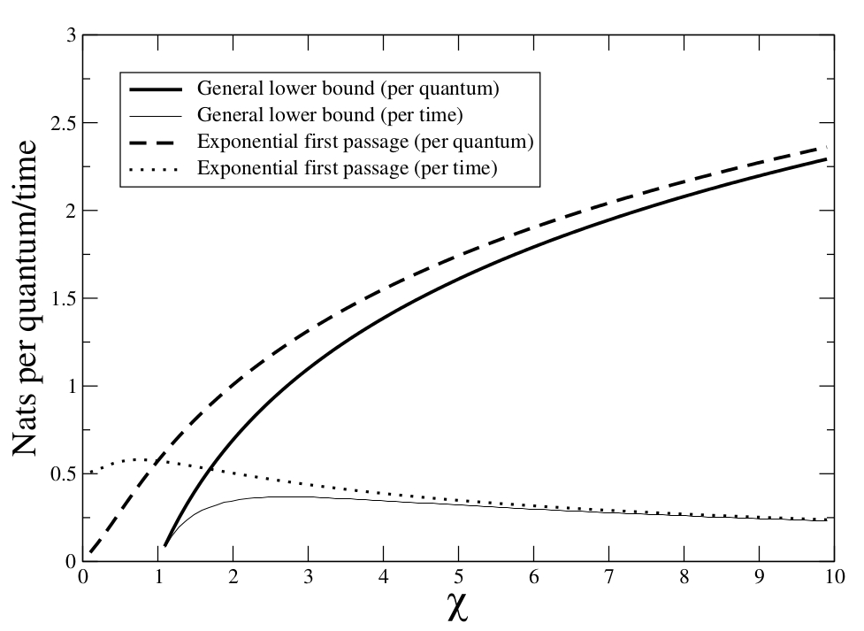
Figure 3: Lower bounds for $C_{q}$ and $C_{t}$ vs. $\chi$.

It is worth noting that free diffusion (brownian motion) first passage times are not finite and thus not well-behaved from an information theoretic capacity standpoint. However, in an finite spatial-extent system, physical constraints on quanta motion enforce finite first passage. It is also noteworthy that by considering quanta in the limit of large $M$ per signaling interval, our results in principle bridge the gap between quantum channel descriptions and signaling agent concentration-based descriptions. That is, though the signaling problem formulation is epoch-based ($M$ quanta per emission period $\tau$, and $\rho=M/\tau$ constant), with large $M$ (and concomitantly large $\tau$), the “instantaneous” concentrations of quanta within an emission period are not so constrained.

The question of quanta number vs. timing information is worth exploring briefly. Consider that instead of fixing the number of quanta per epoch, we might send different numbers of quanta in each epoch. We have shown that $C_{q}(M)$ is at least linear in $M$. In contrast, the maximum amount of information conveyed per epoch by the number of quanta is exactly $\log M$ – strongly sub-linear in $M$. The argument also applies to $C_{t}(M)$ since the guard interval is proportionately larger for small $M$ (larger-$M$ intervals are more temporally efficient and therefore higher rate). Thus, in terms of information transfer, timing information seems strongly preferred, at least asymptotically.

Our lower bounds on channel capacity in nats per quantum (equation (67) and equation (74)) and the corresponding bounds in nats per unit time (equation (70)) are shown FIGURE 3. Increasing $\chi$ increases the emission interval relative the mean first passage time and thereby increases the information content of any individual quantum. In addition, since successive quanta may be less likely to interchange position, $\frac{1}{M}\left(\log M!-H(\Omega|\vec{{\bf S}};{\bf T})\right)$ approaches zero. Thus, the simple lower bound of equation (67) (and correspondingly equation (70)) meets the lower bound for exponential first passage which has minmax $I({\bf S};{\bf T})$. But perhaps most interesting is the implication that there may exist optimum emission rates for a given channel as evidenced by the shape of the $C_{t}$ curves in FIGURE 3. This feature echos [16] where an optimum burst interval for signaling molecules in a diffusive channel was derived. However, since we do not know the channel capacity, we do not know how tight our lower bounds are. It is therefore premature to say whether an optimum emission rate is a feature of the identical quanta timing channel.

References

- [1] O. Milenkovic, G. Alterovitz, G. Battail, T. P. Coleman, J. Hagenauer, S. P. Meyn, N. Price, M. F. Ramoni, I. Shmulevich, and W. Szpankowski. Introduction to the special issue on information theory in molecular biology and neuroscience. Trans. Information Theory, 56(2):649–652, 2010.
- [2] C. de Joussineau, J. Soule, M. Martin, C Anguille, P. Montcourrier, and D. Alexandre. Delta-Promoted Filopodia Mediate Long-Range Lateral Inhibition in Drosophila. Nature, 426:555–559, December 4 2003.
- [3] Y.A. Gorby, S. Yanina, JS.. McLean, K.M. Rosso, D. Moyles, A. Dohnalkova, T.J. Beveridge, I.S. Chang, B.H. Kim, K.S. Kim, D.E. Culley, S.B. Reed, M.F. Romine, D.A. Saffarini, E.A. Hill, L. Shi, D.A. Elias, D.W. Kennedy, G. Pinchuk, K. Watanabe, S. Ishii, B. Logan, K.H. Nealson, and J.K. Fredrickson. Electrically conductive bacterial nanowires produced by Shewanella oneidensis strain MR-1 and other microorganisms. Proc Natl Acad Sci U.S.A., 103:11358–11363, 2006.
- [4] S. Gurke, J.F.V. Barroso, and H.-H. Gerdes. The art of cellular communication: tunneling nanotubes bridge the divide. Histochem Cell Biol, 129:539–550, 2008.
- [5] X. Wang, M.L. Veruki, N.V. Bukoreshtliev, E. Hartveit, and H.-H. Gerdes. Animal cells connected by nanotubes can be electrically coupled through interposed gap-junction channels. Proc Natl Acad Sci USA, 107:17194–17199, 2010.
- [6] H.C. Berg and E.W. Purcell. Physics of Chemoreception. Biophysical Journal, 20:193–219, 1977.
- [7] Pankaj Mehta et al. Information processing and signal integration in bacterial quorum sensing. Molecular systems biology, 2009.
- [8] A.L. Hodgkin and A.F. Huxley. A quantitative description of membrane current and its application to conduction and excitation in nerve. J. Physiol., 117(4):500–544, 1952.
- [9] Tao Long et al. Quantifying the integration of quorum-sensing signals with single-cell resolution. Molecular systems biology, 2009.
- [10] Elek Wajnryb Jose M. Amigo, Janusz Szczepanski and Maria V. Sanchez-Vives. Estimating the entropy rate of spike trains via lempel-ziv complexity. Neural Computation, 16:717–736, 2004.
- [11] D.H. Johnson. Information Theory and Neural Information Processing. Trans. Information Theory, 56(2):653–666, Feb 2010.
- [12] Riccardo Barbieri, Loren M. Frank, David P. Nguyen, Michael C. Quirk, Victor Solo, Matthew A. Wilson, and Emery N. Brown. Dynamic analyses of information encoding in neural ensembles. Neural Computation, 16:277–307, 2004.
- [13] I.S. Mian and C. Rose. Communication theory and multicellular biology. Integrative Biology, 3(4):350–367, April 2011.
- [14] V. Anantharam and S. Verdu. Bits Through Queues. IEEE Transactions on Information Theory, 42(1):4–18, January 1996.
- [15] A.W. Eckford. Nanoscale communication with Brownian motion. In CISS’07, pages 160–165, 2007. Baltimore.
- [16] A. Einolghozati, M. Sardari, A. Beirami, and F. Fekri. Capacity of Discrete Molecular Diffusion Channels. In IEEE International Symposium on Information Theory (ISIT) 2011, pages 603–607, July 2011. ISBN: 978-1-4577-0594-6.
- [17] C. Nusslein-Volhard. Coming to Life: how genes drive development. Kales Press, 2006.
- [18] T.M. Cover and J.A. Thomas. Elements of Information Theory. Wiley-Interscience, 1991.
- [19] F.B. Hildebrand. Advanced Calculus for Applications. Prentice Hall, Englewood Cliffs, NJ, 1976.
- [20] Y-L Tsai, C. Rose, R. Song, and I.S. Mian. An Additive Exponential Noise Channel with a Transmission Deadline. In IEEE International Symposium on Information Theory (ISIT) 2011, pages 598–602, July 2011. ISBN: 978-1-4577-0594-6.
- [21] D.L. Nelson and M.M. Cox. Lehninger Principles of Biochemistry. Freeman, 2005. 4th Ed.
- [22] A. Lehninger. Biochemistry: the Molecular Basis of Cell Structure and Function. Worth Publishing, 1975.
- [23] A. Papoulis. Probability, Random Variables, and Stochastic Processes. McGraw-Hill, New York, third edition, 1991.