WRF fire simulation coupled with a fuel moisture model and smoke transport by WRF-Chem

1 Introduction

We describe two recent additions to SFIRE, a fire spread model coupled with WRF Mandel et al. (2009, 2011). This model builds on the earlier CAWFE code Clark et al. (1996, 2004); Coen (2005); see Mandel et al. (2011) and http://www.openwfm.org/wiki/WRF-Fire_development_notes for further historical details and acknowledgements. The coupled model is available from OpenWFM.org. An earlier version of the code is included in WRF release as WRF-Fire.

2 Fuel moisture model

Fire spread rate depends strongly on the moisture contents of the fuel. In fact, the spread rate drops to zero when the moisture reaches the so-called extinction value Pyne et al. (1996). For this reason, we have coupled the fire spread model with a simple fuel moisture model integrated in SFIRE and run independently at points of the mesh. See Nelson Jr. (2000); Weise et al. (2005) for other, much more sophisticated models. Coen (2005) used an assumed diurnal dependence of fuel moisture on time. Empirical models Fosberg and Deeming (1971); Van Wagner and Pickett (1985) attempt to predict fuel moisture from meteorological conditions measured daily. We use a simple timelag differential equation at every point of the domain. This equations has solutions which approach an equilibrium exponentially, if the equilibrium does not change. In general, the solutions track a changing equilibrium with a delay.

First, relative humidity is computed from the atmospheric temperature $T$ (K), waver vapor contents $Q$ (kg$/$kg), and pressure $P$ (Pa). The saturated water vapor pressure $P_{WS}$ (Pa) is approximated, following (Murphy and Koop 2005, Eq. (10)), as $P_{WS}=\exp(54.842763-6763.22/T-4.210\log T+0.000367T+\tanh\left\{0.0415\left(T-218.8\right)\right\}(53.878-1331.22/T-9.44523\log T+0.014025T)),123<T<332\mathrm{K}$. The water vapor pressure is $P_{W}=PQ/\left(\varepsilon+\left(\ 1-\varepsilon\right)Q\right)$, where $\varepsilon=0.622$ is the ratio of the molecular weight of water ($18.02$ g/mol) to molecular weight of dry air ($28.97$ g/mol). We then obtain the relative humidity $H=100P_{W}/P_{WS}.$The temperature and the relative humidity of the air are then used to estimate the drying and wetting fuel equilibrium moisture contents (Van Wagner and Pickett 1985, eq. (4), (5)) (Viney 1991, eq. (7), (8)),

$$E_{d} =0.924H^{0.679}+0.000499e^{0.1H}+0.18(21.1+273.15-T)(1-e^{-0.115H}),$$

$$E_{w} =0.618H^{0.753}+0.000454e^{0.1H}+0.18(21.1+273.15-T)(1-e^{-0.115H}).$$

The fuel is considered as a combination of time-lag classes, and the fuel moisture contents $m_{k}\left(t\right)$ in each class $k=1,\ldots,N$ is then modeled by the standard time-lag equation

$$\frac{dm_{k}}{dt}=\left\{\begin{array}[c]{c}\frac{E_{d}-m_{k}}{T_{k}}\text{ if }m_{k}>E_{d}\\ 0\text{ if }E_{d}<m_{k}<E_{w}\\ \frac{E_{w}-m_{k}}{T_{k}}\text{ if }m_{k}<E_{w}\end{array}\right.$$ (1)

where $T_{k}$ is the lag time. We use the standard model with the fuel consisting of components with $T_{k}=1$, $10$, and $100$ hour lag time, with the proportions $w_{k}\geq 0,$ $\sum_{k=1}^{N}w_{k}=1$, given by the fuel category description Scott and Burgan (2005). The overall fuel moisture then is the weighted average $m=\sum_{k=1}^{N}w_{k}m_{k}$.

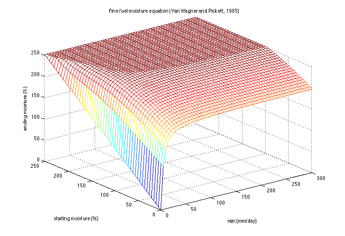
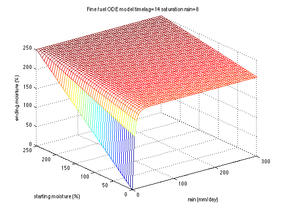
(a)	(b)

Figure 1: Response of fine fuels to rain over 24 hours (a) following Van Wagner and Pickett (1985) (b) from the time-lag model (2) by a calibration of coefficients.

During rain, the equilibrium moisture $E_{d}$ or $E_{w}$ is replaced by the saturation moisture contents $S$, and equation (1) is modified to achieve the rain-wetting lag time $T_{rk}$ for heavy rain only asymptotically, when the rain intensity $r$ (mm/h) is large:

$$\frac{dm_{k}}{dt}=\frac{S-m_{k}}{T_{rk}}\left(1-\exp\left(-\frac{r-r_{0}}{r_{k}}\right)\right),\text{ if }r>r_{0},$$ (2)

where $r_{0}$ is the threshold rain intensity below which no perceptible wetting occurs, and $r_{k}$ is the saturation rain intensity for fuel component $k$. At the saturation rain intensity, $1-1/e\approx 63\%$ of the maximal rain-wetting rate is achieved. The coefficients can be calibrated to achieve a similar behavior as accepted empirical models Fosberg and Deeming (1971); Van Wagner and Pickett (1985). This model estimates the fuel moisture as a function of the initial moisture contents and rain accumulation over 24 hours. Assuming steady rain over the 24 hours, we have obtained a reasonable match with the Canadian fire danger rating system Van Wagner and Pickett (1985) using $S=250\%,T_{rk}=14$ h, $r_{0}=0.05$ mm$/$h and $r_{k}=8$ mm$/$h, cf., Fig. 1. Of course, since fuel may dry up between episodes of rain, in the case of intermittent rain, the result of the model depends also on the temporal rain distribution, not only the total accumulation – just like fuel moisture in reality.

Because we want the model to support an arbitrarily long time step, an adaptive exponential method was implemented. The method is exact for long time step when the atmospheric variables and the rain intensity are constant in time. Equations (1) and (2) have the common form

$$\frac{dm}{dt}=\frac{E-m}{T}.$$ (3)

For longer time steps, use the exact solution of (3) over the time step interfal $\left[t_{n},t_{n+1}\right]$, with constant coefficients taken as their values at $t_{n+1/2}=t_{n}+\Delta t/2$, which gives $M_{n+1}=M_{n}+\left(E_{n+1/2}-M_{n}\right)\left(1-e^{-\Delta t/T_{n+1/2}}\right)$, where $E_{n+1/2}$ and $T_{n+1/2}$ are computed at $t_{n+1/2}$. This method is of second order and it is particularly useful when the time step is comparable to or even larger than the time lag and the coefficients $E$ and $T$ vary slowly, such as in the case of fast drying just after the rain ends. For very short time steps, however, the rounding error in the subtraction of the almost equal quantities in $1-e^{-\Delta t/T_{n+1/2}}$ will pollute the solution. Thus, for $\Delta t/T_{n+1/2}<\varepsilon=0.01$, we replace the exponential by a truncated Taylor expansion, and use the second order method $M_{n+1}=M_{n}+\left(E_{n+1/2}-M_{n}\right)\frac{\Delta t}{T_{n+1/2}}\left(1-\frac{1}{2}\frac{\Delta t}{T_{n+1/2}}\right).$

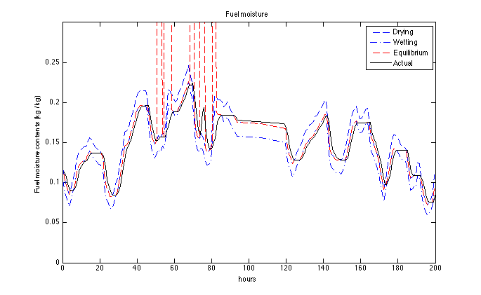
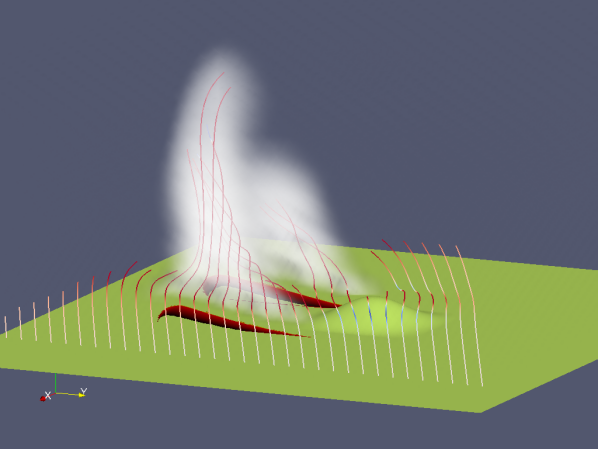
(a)	(b)

Figure 2: (a) Simulation of fuel moisture contents at a single point for fine fuels. The drying and wetting equilibria are computed from the WRF state. The fuel moisture contents does not change when it is between the two equilibria. The red vertical lines correspond to periods of rain, where the equilibrium is 2.5 (above the range shown). The fuel moisture contents increases during rain and exhibits diurnal variability. The flat part between 100 and 200 hours is due to one day of missing data. (b) Advection of smoke by tracers injected in WRF-Chem, in an ideal example.

Because the time scale of the moisture changes (hours) is very different from the time scales of the atmoshere (minutes( and fire (seconds), the moisture model runs at a multiple of the WRF time step. WRF variables P (pressure, Pa), T2 (temperature at 2m, K), and Q2 (water vapor mixing ratio, kg/kg) at the beginning and the end of the moisture model time step are averaged to obtain the values of $P$, $T$, and $Q$ used in the timestep of the moisture model,

$$P_{n+1/2}=\frac{\mathtt{P}\left(t_{n+1}\right)+\mathtt{P}\left(t_{n}\right)}{2},\quad T_{n+1/2}=\frac{\mathtt{T2}\left(t_{n+1}\right)+\mathtt{T2}\left(t_{n}\right)}{2},\quad Q_{nn+1/2}=\frac{\mathtt{Q2}\left(t_{n+1}\right)+\mathtt{Q2}\left(t_{n}\right)}{2},$$

This is done for 2nd order accuracy as well as for compatibility with the computation of the rain intensity from the difference of the accumulated rain,

$$r_{n+1/2}=\frac{\mathtt{RAINC}(t_{n+1})+\mathtt{RAINNC}\left(t_{n+1}\right)-\mathtt{RAINC}(t_{n})-\mathtt{RAINNC}\left(t_{n}\right)}{\Delta t}.$$

These values are then used to compute the equilibrium moisture contents and the time lag, and one time step is performed, as described above. See Fig. 2i(a) for a typical simulation result.

The fire model runs on a finer grid than the atmospheric model, typically refined by a factor of $10$ or more. The moisture model consists of two steps.

In the first step, we compute the moisture content $m_{k}$ of the fuel components on the nodes of the atmospheric grid on the Earth surface for several reasons. (1) The WRF variables are known at the nodes of the atmospheric grid and no interpolation is needed. (2) The atmospheric grid is relatively coarse, so the added costs of storage of several surface moisture fields $m_{k}$ and of the computation are not significant. (3) The computation is done for each fuel component indivudually over the whole domain and it does not depend on the actual fuel map. (4) The fire model does not need to run for the computation of $m_{k}$.

In the second step, we interpolate the values of $m_{k}$ to the fire grid and compute the weighted averages on the fire grid following using the actual fuel map. There are several options how to run the fuel moisture model: (1) Turn on both steps of the moisture model: compute the moisture fields $m_{k}$ and interpolate on the fire grid, as the fire model runs. This option is intended for the actual fire simulation. (2) Turn on the first step, computation of the moisture fields $m_{k}$ only, for an extended run (many days) to evolve the $m_{k}$ in response to the simulated weather, into a dynamic equilibrium. The moisture fields are stored in WRF state in the output and the restart files. (3) Run the first step, computation of the moisture fields $m_{k}$, as a standalone executable from stored output files from standard WRF runs, adding the moisture fields $m_{k}$ to the files. (4) Start the coupled atmosphere-fire-moisture simulation from the moisture fields evolved over time as above. (5) Run the fire model as a standalone exectutable, without feedback on the atmosphere, with fuel moisture computed using the second step only from the fields $m_{k}$ in WRF output files produced in advance.

3 Coupling with WRF-Chem

Coupling with WRF-Chem is implemented by inserting the smoke intensity in the WRF-Chem arrays emis_ant and tracer at the ground layer and with the species index p_smoke. WRF needs to be configured with the chem option and built with em_fire or em_real, and the appropriate options trace_opt=1 and chem_opt=14 set in the namelist. A sample visualization of an ideal run with smoke transport is in Fig. 2(b). See the WRF SFIRE Users’ Guide at http://www.openwfm.org/wiki/Users_guide for further details and more information as the code develops further.

Currently, the smoke inserted into WRF-Chem is simply proportional to the fire heat flux. However, a more sophisticated scheme following the FEPS (Fire Emission Production Simulator) is being implemented Anderson et al. (2004). In this new method, the fire emission will be treated as the fluxes of carbon dioxide (CO2), carbon monoxide (CO), methane (CH4) and particulate matter (PM 2.5) released into the atmosphere at the location of the fire. The total emission for each of these species will be computed based on the fuel burn rate (amount of fuel burnt per unit time), fuel load, and the smoldering correction computed based from the wind speed and relative humidity. The PM 2.5 will be portioned into the the accumulation and nuclei mode and released into the atmosphere as PM25J and PM25I respectively.

Aside from the obvious application to smoke dispersal, which is important in practice, taking into account the composition of the fire emitted smoke will allow for treating it as chemically and physically active. The species released into the atmosphere by the fire will undergo chemical reactions allowing for capturing the secondary aerosol effects. The particular mater will interact with atmospheric radiation, and have a potential to serve as condensation nuclei when suitable cloud microphysics is available. This may be of great importance in the simulation of visible plumes and pyrocumulus clouds, under development in Peace et al. (2011).

References

- Anderson et al. (2004) Anderson, G. K., D. V. Sandberg, and R. A. Norheim, 2004: Fire emission production simulator (FEPS) user’s guide version 1.0. USDA Forest Service, PNW Research Station, http://www.fs.fed.us/pnw/fera/feps/FEPS_users_guide.pdf.
- Clark et al. (2004) Clark, T. L., J. Coen, and D. Latham, 2004: Description of a coupled atmosphere-fire model. International Journal of Wildland Fire, 13, 49–64, doi:10.1071/WF03043.
- Clark et al. (1996) Clark, T. L., M. A. Jenkins, J. Coen, and D. Packham, 1996: A coupled atmospheric-fire model: Convective feedback on fire line dynamics. Journal of Applied Meteorolgy, 35, 875–901, doi:10.1175/1520-0450(1996)0350875:ACAMCF2.0.CO;2.
- Coen (2005) Coen, J. L., 2005: Simulation of the Big Elk Fire using coupled atmosphere-fire modeling. International Journal of Wildland Fire, 14, 49–59, doi:10.1071/WF04047.
- Fosberg and Deeming (1971) Fosberg, M. A. and J. E. Deeming, 1971: Derivation of the 1- and 10-hour timelag fuel moisture calculations for fire-danger rating. U.S. Forest Service Research Note RM-207, http://hdl.handle.net/2027/umn.31951d02995763p.
- Mandel et al. (2009) Mandel, J., J. D. Beezley, J. L. Coen, and M. Kim, 2009: Data assimilation for wildland fires: Ensemble Kalman filters in coupled atmosphere-surface models. IEEE Control Systems Magazine, 29, 47–65, doi:10.1109/MCS.2009.932224.
- Mandel et al. (2011) Mandel, J., J. D. Beezley, and A. K. Kochanski, 2011: Coupled atmosphere-wildland fire modeling with WRF 3.3 and SFIRE 2011. Geoscientific Model Development, 4, 591–610, doi:10.5194/gmd-4-591-2011.
- Murphy and Koop (2005) Murphy, D. M. and T. Koop, 2005: Review of the vapour pressures of ice and supercooled water for atmospheric applications. Q. J. R. Meteorol. Soc., 131, 1539–1565, doi:10.1256/qj.04.94.
- Nelson Jr. (2000) Nelson Jr., R. M., 2000: Prediction of diurnal change in 10-h fuel stick moisture content. Canadian Journal of Forest Research, 30, 1071–1087, doi:10.1139/x00-032.
- Peace et al. (2011) Peace, M., T. Mattner, and G. Mills, 2011: Case studies and preliminary WRF-fire simulations of two bushfires in sea breeze convergence zones. Paper 3.3, Ninth Symposium on Fire and Forest Meteorology, Palm Springs, October 2011, http://ams.confex.com/ams/9FIRE/webprogram/Paper192200.html, retrieved June 2012.
- Pyne et al. (1996) Pyne, S., P. L. Andrews, and R. D. Laven, 1996: Introduction to Wildland Fire. Wiley, New York.
- Scott and Burgan (2005) Scott, J. H. and R. E. Burgan, 2005: Standard fire behavior fuel models: A comprehensive set for use with Rothermel’s surface fire spread model. Gen. Tech. Rep. RMRS-GTR-153. Fort Collins, CO: U.S. Department of Agriculture, Forest Service, Rocky Mountain Research Station, http://www.fs.fed.us/rm/pubs/rmrs_gtr153.html.
- Van Wagner and Pickett (1985) Van Wagner, C. E. and T. L. Pickett, 1985: Equations and FORTRAN program for the Canadian forest fire weather index system. Canadian Forestry Service, Forestry Technical Report 33.
- Viney (1991) Viney, N. R., 1991: A review of fine fuel moisture modelling. International Journal of Wildland Fire, 1, 215–234, doi:10.1071/WF9910215.
- Weise et al. (2005) Weise, D. R., F. M. Fujioka, and R. M. Nelson Jr., 2005: A comparison of three models of 1-h time lag fuel moisture in Hawaii. Agricultural and Forest Meteorology, 133, 28–39, doi:10.1016/j.agrformet.2005.03.012.