Parallelization, processor communication and error analysis in lattice kinetic Monte Carlo

Abstract

In this paper we study from a numerical analysis perspective the Fractional Step Kinetic Monte Carlo (FS-KMC) algorithms proposed in [1] for the parallel simulation of spatially distributed particle systems on a lattice. FS-KMC are fractional step algorithms with a time-stepping window $\Delta t$, and as such they are inherently partially asynchronous since there is no processor communication during the period $\Delta t$. In this contribution we primarily focus on the error analysis of FS-KMC algorithms as approximations of conventional, serial kinetic Monte Carlo (KMC). A key aspect of our analysis relies on emphasizing a goal-oriented approach for suitably defined macroscopic observables (e.g., density, energy, correlations, surface roughness), rather than focusing on strong topology estimates for individual trajectories.

One of the key implications of our error analysis is that it allows us to address systematically the processor communication of different parallelization strategies for KMC by comparing their (partial) asynchrony, which in turn is measured by their respective fractional time step $\Delta t$ for a prescribed error tolerance.

1 Introduction

The simulation of stochastic lattice systems using kinetic Monte Carlo (KMC) methods relies on the direct numerical simulation of the underlying Continuous Time Markov Chain (CTMC). In [1] we proposed a new mathematical and computational framework for constructing parallel algorithms for KMC simulations.The parallel algorithms in [1] are controlled approximations of Kinetic Monte Carlo algorithms, and rely on first developing a spatio-temporal decomposition of the Markov operator for the underlying CTMC into a hierarchy of operators corresponding to the particular parallel architecture. Based on this operator decomposition, we formulated Fractional Step Approximation schemes by employing the Trotter product formula, which in turn determines the processor communication schedule. The fractional step framework allows for a hierarchical structure to be easily formulated and implemented, offering a key advantage for simulating on modern parallel architectures with elaborate memory and processor hierarchies. The resulting parallel algorithms are inherently partially asynchronous as processors do not communicate during the fractional time step window $\Delta t$.

Earlier, in [23] the authors also proposed an approximate algorithm, in order to create a parallelization scheme for KMC. It was demonstrated in [19, 20], that boundary inconsistencies are resolved in a straightforward fashion, while there is an absence of global communications. Finally, among the parallel algorithms tested in [19], the one in [23] had the highest parallel efficiency. In [1], we demonstrated that the approximate algorithm in [23] is a special case of the Fractional Step Approximation schemes introduced in [1]. There we also demonstrated, using the Random Trotter Theorem [13], that the algorithm in [23] is numerically consistent in the approximation limit, i.e., as the time step in the fractional step scheme converges to zero, it converges to a Markov Chain that has the same master equation and generator as the original serial KMC. The open source SPPARKS parallel Kinetic Monte Carlo simulator, [20], can also be formulated as a Fractional Step approximation. In this article, the convergence, reliability and efficiency of all such Fractional Step KMC parallelization methods is systematically explored by rigorous numerical analysis which relies on controlled-error approximations in transient regimes relevant to the simulation of extended systems.

A key aspect of the presented analysis relies on emphasizing a goal-oriented error approach for suitably defined macroscopic observables, e.g., density, energy, correlations, surface roughness , giving rise to estimates which are independent of the (very large) system size of the particle system. Besides the obtained numerical consistency and reliability of the approximating CTMC obtained from FS-KMC there is an additional key practical point: the bigger is the allowable $\Delta t$, within a desired error tolerance, the less processor communication is required. From a broader mathematical perspective, and driven from parallel computing challenges, the developed mathematical and numerical analysis attempts to balance between controlled error approximations and processor communication. The same methods could also prove useful for developing and evaluating parallel numerical schemes for other molecular and extended systems.

2 Background

Kinetic Monte Carlo (KMC) algorithms have proved to be an important tool for the simulation of non-equilibrium, spatially distributed chemical processes arising in applications ranging from materials science, catalysis and reaction engineering, to complex biological processes. Typically the simulated models involve chemistry and/or transport micro-mechanisms for atoms and molecules, e.g., reactions, adsorption, desorption processes and diffusion on surfaces and through porous media, [14, 2, 4]. Furthermore, mathematically similar mechanisms and corresponding KMC simulations arise in agent-based models in epidemiology, ecology and traffic networks, [24].

We consider an interacting particle system defined on a $d$-dimensional lattice ${\Lambda}_{N}$. Naturally, the simulations are performed on a finite lattice of the size $N$, however, given the size of real molecular systems it is either necessary to treat the case $N\to\infty$, e.g., $\Lambda=\mathbb{Z}^{d}$, or alternatively any numerical estimates we obtain need to be independent of the system size $N$. We restrict our discussion to lattice gas models where the order parameter or the spin variable takes values in a compact set, in most cases the set is finite $\Sigma=\{0,1,\dots,{K}\}$. At each lattice site $x\in{\Lambda}_{N}$ an order parameter (a spin variable) $\sigma(x)\in\Sigma$ is defined. The states in $\Sigma$ correspond to occupation of the site $x\in{\Lambda}_{N}$ by different species. For example, if $\Sigma=\{0,1\}$ the order parameter models the classical lattice gas with a single species occupying the site $x$ when $\sigma(x)=1$ and with the site being vacant if $\sigma(x)=0$. We denote $\{\sigma_{t}\}_{t\geq 0}$ the stochastic process with values in the countable configuration space ${\mathcal{S}}=\Sigma^{{\Lambda}_{N}}$. Microscopic dynamics is described by transitions (changes) of spin variables at different sites. We study systems in which the transitions are localized and involve only finite number of sites at each transition step. First, the local dynamics is described by an updating mechanism and corresponding transition rates $c(x,\omega;\sigma)$ in (1), such that the configuration at time $t$, $\sigma_{t}=\sigma$ changes into a new configuration $\sigma^{x,\omega}$ by an update in a neighborhood of the site $x\in{\Lambda}_{N}$. Here $\omega\in{\mathcal{S}}_{x}$, where ${\mathcal{S}}_{x}$ is the set of all possible configurations that correspond to an update at a neighborhood $\Omega_{x}$ of the site $x$. For example, if the modeled process is a diffusion of the classical lattice gas a particle at $x$, i.e., $\sigma(x)$ can move to any unoccupied nearest neighbor $y$ of $x$, i.e., $\Omega_{x}=\{y\in{\Lambda}_{N}{\,|\,}|x-y|=1\}$ and ${\mathcal{S}}_{x}$ is the set of all possible configurations ${\mathcal{S}}_{x}=\Sigma^{\Omega_{x}}$. Computationally the sample paths $\{\sigma_{t}\}_{t\geq 0}$ are constructed via KMC, that is through the procedure described in (2) and (3) below.

The studied stochastic processes are set on a lattice (square, hexagonal, etc.) ${\Lambda}_{N}$ with $N$ sites, they have a discrete, albeit high-dimensional, configuration space ${\mathcal{S}}$ and necessarily have to be of jump type describing transitions between different configurations $\sigma\in{\mathcal{S}}$. Mathematically, a CTMC is a stochastic process $\{\sigma_{t}\}$ defined completely in terms of the local transition rates $c(\sigma,\sigma^{\prime})$ which determine the updates (jumps) from any current state $\sigma_{t}=\sigma$ to a (random) new state $\sigma^{\prime}$. In the context of the spatially distributed applications in which we are interested here, the local transition rates will be denoted as

$$c(\sigma,\sigma^{\prime})=c(x,\omega;\sigma)\,,$$ (1)

which correspond to an updating micro-mechanism from a current configuration $\sigma_{t}=\sigma$ of the system to a new configuration $\sigma^{x,\omega}$ by performing an update in a neighborhood of each site $x\in{\Lambda}_{N}$. Here $\omega$ is an index for all possible configurations ${\mathcal{S}}_{x}$ that correspond to an update at a neighborhood $\Omega_{x}$ of the site $x$; we refer to the end of the section for specific examples.

The probability of a transition over an infinitesimal time interval ${\delta t}$ is

$${\mathbb{P}\left({\sigma_{t+{\delta t}}=\sigma^{x,\omega}{\,|\,}\sigma_{t}=\sigma}\right)}=c(x,\omega;\sigma){\delta t}+\mathrm{o}({\delta t})\,.$$

Realizations of the process are constructed from the embedded discrete time Markov chain $S_{n}=\sigma_{t_{n}}$ (see [11]), corresponding to jump times $t_{n}$. The local transition rates (1) define the total rate

$$\lambda(\sigma)=\sum_{x\in{\Lambda}_{N}}\sum_{\omega\in{\mathcal{S}}_{x}}c(x,\omega;\sigma)\,,$$ (2)

which is the intensity of the exponential waiting time for a jump from the state $\sigma$. The transition probabilities for the embedded Markov chain $\{S_{n}\}_{n\geq 0}$ are

$$p(\sigma,\sigma^{x,\omega})=\frac{c(x,\omega;\sigma)}{\lambda(\sigma)}\,.$$ (3)

In other words once the exponential “clock” signals a jump, the system transitions from the state $\sigma$ to a new configuration $\sigma^{x,\omega}$ with the probability $p(\sigma,\sigma^{x,\omega})$. On the other hand, the evolution of the entire system at any time $t$ is described by the transition probabilities $P(\sigma,t;\zeta):={\mathbb{P}\left({\sigma_{t}=\sigma{\,|\,}\sigma_{0}=\zeta}\right)}$ where $\zeta\in{\mathcal{S}}$ is an initial configuration. The transition probabilities corresponding to the local rates (1) satisfy the Forward Kolmogorov Equation (Master Equation), [15, 6],

$$\partial_{t}P(\sigma,t;\zeta):=\sum_{\sigma^{\prime},\sigma^{\prime}\neq\sigma}c(\sigma^{\prime},\sigma)P(\sigma^{\prime},t;\zeta)-\lambda(\sigma)P(\sigma,t;\zeta)\,,$$ (4)

where $P(\sigma,0;\zeta)=\delta(\sigma-\zeta)$ and $\delta(\sigma-\zeta)=1$ if $\sigma=\zeta$ and zero otherwise.

In [1] we developed a general mathematical framework for parallelizable approximations of the KMC algorithm. Rather than focusing on exactly constructing stochastic trajectories in (2) and (3), we proposed to approximate the evolution of observables $f=f(\sigma)\in C_{b}({{\mathcal{S}}})$, i.e., of bounded continous functions on the configuration space ${\mathcal{S}}$. The space of bounded continuous functions, $C_{b}({{\mathcal{S}}})$, is regarded as a Banach space with the norm

$$\|\,f\,\|_{\infty}=\sup_{\sigma\in{\mathcal{S}}}|f(\sigma)|\,.$$

Here we consider observables/functions $f(\sigma)$ depending on large number of variables $\sigma(x)$, $x\in{\Lambda}_{N}$, such as coverage, surface roughness, correlations, etc., see for instance the examples in Section 5. Alternatively, we may consider observables depending on infinitely many variables $\sigma(x)$, $x\in\Lambda=\mathbb{Z}^{d}$, to stress the necessity of working with the infinite volume limit.

Typically in KMC we need to compute expected values of such observables, that is quantities such as

$$u(\zeta,t):={\mathbb{E}}^{\zeta}[f(\sigma_{t})]=\sum_{\sigma}f(\sigma)P(\sigma,t;\zeta)\,,$$ (5)

conditioned on the initial data $\sigma_{0}=\zeta$. By a straightforward calculation using (4) we obtain that the observable (5) satisfies the initial value problem

$$\partial_{t}u(\zeta,t)=\mathcal{L}u(\zeta,t)\,,\quad\quad u(\zeta,0)=f(\zeta)\,,$$ (6)

where the operator $\mathcal{L}:C_{b}({\mathcal{S}})\to C_{b}({\mathcal{S}})$ is known as the generator of the continous time Markov chain, [15], and in the case of (1) it is

$$\mathcal{L}f(\sigma)=\sum_{\sigma^{\prime}}c(\sigma,\sigma^{\prime})[f(\sigma^{\prime})-f(\sigma)]=\sum_{x\in{\Lambda}_{N}}\sum_{\omega\in{\mathcal{S}}_{x}}c(x,\omega;\sigma)[f(\sigma^{x,\omega})-f(\sigma)]\,.$$ (7)

We then write (5), as the the action of the Markov semi-group $e^{t\mathcal{L}}$ associated with the generator $\mathcal{L}$ and the process $\{{\sigma_{t}}\}_{t\geq 0}$, [15], on the observable $f$

$$u(\zeta,t)={\mathbb{E}}^{\zeta}[f(\sigma_{t})]=e^{t\mathcal{L}}f(\zeta)\,,$$ (8)

where ${\mathbb{E}}^{\zeta}$ denotes the expected value with respect to the law of the process $\{\sigma_{t}\}_{t\geq 0}$ conditioned on the initial configuration $\zeta$.

We define a difference operator $\delta_{x}f$ as an analogue of a derivative. Higher-order derivative analogues are defined in Section 5 when needed in the error analysis. We define a corresponding function space, which is necessary in order to set up the semigroup $P=e^{t\mathcal{L}}$ when we consider the infinite lattice $\Lambda=\mathbb{Z}^{d}$ or to obtain estimates which are independent of the system size $N$ when considering the lattice ${\Lambda}_{N}$ in Section 5.

Definition 1.

Let $f\in C_{b}({{\mathcal{S}}})$ then for any $x\in{\Lambda}_{N}$ we define

$$\delta_{x,\omega}f(\sigma)=f(\sigma^{x,\omega})-f(\sigma)\,.$$

We define the norm

$$\|{f}\|_{1}\equiv\sum_{x,\omega}\|\,\delta_{x,\omega}f\,\|_{\infty}$$

and the space of functions on ${\mathcal{S}}=\Sigma^{{\Lambda}_{N}}$

$$C^{1}({{\mathcal{S}}})=\{f\in C_{b}({\mathcal{S}}){\,|\,}\|{f}\|_{1}\leq C_{f}\;\;\mathrm{where}\;\;C_{f}\;\;\mathrm{is\;independent\;of}\;\;N\ \}\,.$$

Similarly we define the space of functions on ${\mathcal{S}}=\Sigma^{\Lambda}$ associated with the infinite lattice $\Lambda=\mathbb{Z}^{d}$

$$C^{1}({{\mathcal{S}}})=\{f\in C_{b}({\mathcal{S}}){\,|\,}\|{f}\|_{1}<\infty\}\,.$$

Because of the estimates in Section 5, see (31) and (33) in Theorem 13, we will employ spaces with higher discrete derivatives that will be defined in Section 5. On the infinite lattice $\Lambda$ macroscopic observables are all $f\in C^{1}({{\mathcal{S}}})$. In the case of ${\Lambda}_{N}$, macroscopic observables are all $f=f(\sigma)$ such that $\|{f}\|_{1}$ is independent of the system size $N$; such typical examples are discussed in Section 5.

Typically, the evolution of the particle system on the infinite lattice $\Lambda=\mathbb{Z}^{d}$ is well-defined, as demonstrated in the next propositions.

Proposition 2.

For any $f\in C^{1}({{\mathcal{S}}})$ we have that the series

$$\mathcal{L}f(\sigma)=\sum_{x\in\Lambda}\sum_{\omega\in{\mathcal{S}}_{x}}c(x,\omega;\sigma)[f(\sigma^{x,\omega})-f(\sigma)]\,,$$

converges uniformly and defines a function in $C_{b}({\mathcal{S}})$, provided $\sup_{{x,\omega},\sigma}c(x,\omega;\sigma)<\infty$. Furthermore,

$$\|\,\mathcal{L}f\,\|_{\infty}\leq\sup_{{x,\omega},\sigma}c(x,\omega;\sigma)\|{f}\|_{1}\,.$$

Proof.

Follows directly from (7) and the definition of $C^{1}({{\mathcal{S}}})$. $\Box$

Proposition 3.

Under the boundedness assumptions on the rates, the closure of the operator $\mathcal{L}$ defines a Markov generator for a Markov semigroup $P\equiv e^{t\mathcal{L}}$, such that for $f\in C^{1}({{\mathcal{S}}})$, $Pf\in C^{1}({{\mathcal{S}}})$ and

$$\|{e^{t\mathcal{L}}f}\|_{1}\leq e^{\Gamma t}\|{f}\|_{1}\,,$$

where $\Gamma$ is a constant depending on the rates $c(x,\omega;\sigma)$.

Proof.

See [15, Theorem 3.9, pp 27]. $\Box$

Clearly the same results hold for the finite lattice ${\Lambda}_{N}$ and the corresponding high-dimensional configuration space ${\mathcal{S}}$, where all constants are independent of the size $N$.

Examples.
Adsorption/Desorption for single species particles. In this case spins take values in $\sigma(x)\in\Sigma=\{0,1\}$, $\Omega_{x}=\{x\}$, ${\mathcal{S}}_{x}=\{0,1\}$ and the update represents a spin flip at the site $x$, i.e., for $z\in{\Lambda}_{N}$

$$\sigma^{x,\omega}(z)\equiv\sigma^{x}(z)=\begin{cases}\sigma(z)&\mbox{if $z\neq x$,}\\ 1-\sigma(x)&\mbox{if $z=x$.}\end{cases}$$

Diffusion for single species particles. The state space for spins is $\sigma(x)\in\Sigma=\{0,1\}$, $\Omega_{x}=\{y\in{\Lambda}_{N}{\,|\,}|x-y|=1\}$ includes all nearest neighbors of the site $x$ to which a particle can move. Thus the new configuration $\sigma^{x,\omega}=\sigma^{(x,y)}$ is obtained by updating the configuration $\sigma_{t}=\sigma$ from the set of possible local configuration changes $\{0,1\}^{\Omega_{x}}$ using the specific rule, also known as spin exchange, which involves changes at two sites $x$ and $y\in\Omega_{x}$

$$\sigma^{x,\omega}(z)\equiv\sigma^{(x,y)}(z)=\begin{cases}\sigma(z)&\mbox{if $z\neq x,y$,}\\ \sigma(x)&\mbox{if $z=y$,}\\ \sigma(y)&\mbox{if $z=x$.}\end{cases}$$

The transition rate is then written as $c(x,\omega;\sigma)=c(x,y;\sigma)$. The resulting process $\{\sigma_{t}\}_{t\geq 0}$ defines dynamics with the total number of particles ($\sum_{x\in{\Lambda}_{N}}\sigma(x)$) conserved, sometimes referred to as Kawasaki dynamics, [4].

Multicomponent reactions. Reactions that involve ${K}$ species of particles are easily described by enlarging the spin space to $\Sigma=\{0,1,\dots,{K}\}$. If the reactions occur only at a single site $x$, the local configuration space ${\mathcal{S}}_{x}=\Sigma$ and the update is indexed by $k\in\Sigma$ with the rule

$$\sigma^{x,\omega}(z)\equiv\sigma^{(x,k)}(z)=\begin{cases}\sigma(z)&\mbox{if $z\neq x,y$,}\\ k&\mbox{if $z=x$.}\end{cases}$$

The rates $c(x,\omega;\sigma)\equiv c(x,k;\sigma)$ define probability of a transition $\sigma(x)$ to species $k=1,\dots,{K}$ or vacating a site, i.e., $k=0$, over ${\delta t}$.

Reactions involving particles with internal degrees of freedom. Typically a reaction involves particles with internal degrees of freedom, and in this case several neighboring lattice sites may be updated at the same time, corresponding to the degrees of freedom of the particles involved in the reaction. For example, in a case such as CO oxidation on a catalytic surface, [16], when only particles at a nearest-neighbor distance can react we set $\sigma(x)\in\Sigma=\{0,1,\dots,{K}\}$, $\Omega_{x}=\{y\in{\Lambda}_{N}{\,|\,}|x-y|=1\}$ and the set of local updates ${\mathcal{S}}_{x}=\Sigma^{\Omega_{x}}$. Such ${\mathcal{S}}_{x}$ contains all possible reactions in a neighborhood of $x$. When reactions involve only pairs of species, the rates can be indexed by $k$, $l\in\Sigma$, or equivalently ${\mathcal{S}}_{x}=\Sigma\times\Sigma$. Then the reaction rate $c(x,\omega;\sigma)=c(x,y,k,l;\sigma)$ describes the probability per unit time of $\sigma(x)\to k$ at the site $x$ and $\sigma(y)\to l$ at $y$, i.e., the updating mechanism

$$\sigma^{x,\omega}(z)\equiv\sigma^{(x,y,k,l)}(z)=\begin{cases}\sigma(z)&\mbox{if $z\neq x,y$,}\\ k&\mbox{if $z=x$,}\\ l&\mbox{if $z=y$,}\end{cases}$$

where $|x-y|=1$.

3 Towards parallel kinetic Monte Carlo algorithms

In practice, the sample paths $\{\sigma_{t}\}_{t\geq 0}$ are constructed by the kinetic Monte Carlo algorithm, that is by simulating the embedded Markov chain defined by (2) and (3) and advancing the tine by random time-steps from the exponential distribution. Implementations are based on the efficient calculation of transition probabilities, e.g., [3] for Ising models, known as a BKL Algorithm, and in [7] known as Stochastic Simulation Algorithm (SSA) for reaction systems.

It is evident from formulas (2) and (3), that KMC algorithms are inherently serial as updates are done at one site $x\in{\Lambda}_{N}$ at a time, while on the other hand (2) depends on information from the entire spatial domain ${\Lambda}_{N}$. For these reasons it appears that KMC cannot be parallelized easily. However, Lubachevsky, in [17], proposed an asynchronous approach for parallel KMC simulation in the context of Ising systems, in the sense that different processors simulate independently parts of the physical domain, while inconsistencies at the boundaries are corrected with a series of suitable rollbacks. This method relies on the uniformization of (2); thus the approach yields a null-event algorithm, [14], which includes rejected moves over the entire spatial sub-domain that corresponds to each processor, see also [9]. A modification in order to incorporate the BKL Algorithm was proposed in [17], which was implemented and tested in [12]. This is a still asynchronous algorithm, where BKL-type rejection-free simulations are carried out in the interior of each sub-domain (processor), while uniform rates are used at the boundaries, reducing rejections to just the boundary set. However, these asynchronous algorithms may still have a high number of rejections for boundary events and rollbacks, which considerably reduce the parallel efficiency, [22]. Advancing processors in time in a synchronous manner over a fixed time-window can provide a way to mitigate the excessive number of boundary inconsistencies between processors and ensuing rejections and rollbacks in earlier methods. Such synchronous parallel KMC algorithms were proposed in [5], [22], [18], [19]. However, several costly global communications are required at each cycle between all processors whenever a boundary event occurs in any one of them, in order to avoid errors in processor communication, [19]. As we will discuss in the sequel, many of these issues with parallel KMC can be addressed by abandoning the earlier perspective on creating a parallel KMC algorithm with exactly the same rates $c(x,\omega;\sigma)$ in (7) as the serial algorithm.

Indeed, in [1], we adopted the approach of creating a parallel KMC algorithm which approximates the underlying continuous time Markov chain of the serial algorithm instead of reproducing its master equation exactly. We proposed a spatio-temporal decomposition for the Markov operator underlying the KMC algorithm into a hierarchy of operators corresponding to the processor architecture. Based on this operator decomposition we can formulate Fractional Step KMC Approximation schemes by employing the Trotter product formula. In turn these approximating schemes determine the Communication Schedule between processors through the sequential application of the operators in the decomposition, as well as the time step employed in the particular fractional step scheme. Earlier, in [23] the authors also proposed an approximate algorithm, in order to create a parallelization scheme for KMC. It was demonstrated in [19, 20], that boundary inconsistencies are resolved in a straightforward fashion, while there is an absence of global communications. Finally, among the parallel algorithms tested in [19], the one in [23] had the highest parallel efficiency. In [1], we demonstrated that the approximate algorithm in [23] is a special case of the Fractional Step Approximation schemes introduced in [1]. We also demonstrated, using the Random Trotter Theorem, [13], that the algorithm in [23] is numerically consistent in the approximation limit, i.e., as the time step in the fractional step scheme converges to zero, it converges to a Markov Chain that has the same master equation and generator as the original serial KMC. Finally, the open source SPPARKS parallel Kinetic Monte Carlo simulator, [20], also relies on such Fractional Step approximations.

In this article, the convergence, reliability and efficiency of parallel algorithms, that fit the Fractional Step KMC approximation framework, are systematically explored by rigorous numerical analysis which relies on controlled-error approximations in transient regimes relevant to the simulation of extended systems.

3.1 Fractional time step kinetic Monte Carlo algorithms

In [1] we proposed a class of parallel KMC algorithms that are based on operator splitting of the Markov generator $\mathcal{L}$ which is based on a geometric decomposition of the lattice ${\Lambda}_{N}$.

Definition 4.

The lattice ${\Lambda}_{N}$ is decomposed into non-overlapping coarse cells $C_{m}$, $m=1,\dots,M$ such that, $|C_{m}|=Q=q^{d}$, where $d$ is the dimension,

$${\Lambda}_{N}=\bigcup_{m=1}^{M}C_{m}\,,\;\;\;\;C_{m}\cap C_{n}=\emptyset\,,\;m\neq n\,,\;N=MQ\,.$$ (9)

The range of interactions is defined as $L=\max_{x\in C_{m}}\{\mathrm{diam}\,\Omega_{x}\}$. For a coarse cell $C_{m}$ the closure of this set is

$$\bar{C}_{m}=\{z\in{\Lambda}_{N}{\,|\,}|z-x|\leq L\,,x\in C_{m}\}\,.$$

The boundary of $C_{m}$ is then defined as $\partial C_{m}=\bar{C}_{m}\;\setminus\;C_{m}$.

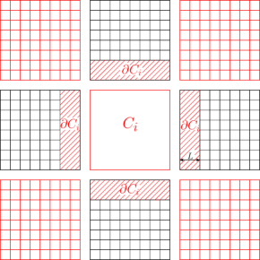
The closure $\bar{C}_{m}$ thus includes all sites of $C_{m}$ and all “boundary” lattice sites $\partial C_{m}$ which are connected with sites in $C_{m}$ through particle interactions in the updating mechanism, see Figure 1. In many models the value of the interaction range $L$ is independent of $x$ due to the translational invariance of the model. This geometric partitioning induces a decomposition of (7)

$$\mathcal{L}f(\sigma)=\sum_{m=1}^{M}\mathcal{L}_{m}f(\sigma)\,,\quad\quad\mathcal{L}_{m}f(\sigma)=\sum_{x\in C_{m}}\sum_{x,\omega\in{\mathcal{S}}_{x}}c(\omega;\sigma)[f(\sigma^{x,\omega})-f(\sigma)]\,.$$ (10)

The generators $\mathcal{L}_{m}$ define a new Markov process $\{\sigma^{m}_{t}\}_{t\geq 0}$ on the entire lattice ${\Lambda}_{N}$.

Remark 3.1.

In many models such as in catalysis the interactions between particles are short-range, [21, 16], and therefore the transition rates $c(x,\omega;\sigma)$ depend on the configuration $\sigma$ only through $\sigma(x)$ and $\sigma(y)$ with $|x-y|\leq L$, where $L$ is small (typically one). Similarly the new configuration $\sigma^{x,\omega}$ involves changes only at the sites in this neighborhood. Thus the generator $\mathcal{L}_{m}$ updates the lattice sites at most in the set $\bar{C}_{m}=\{z{\,|\,}|x-z|\leq L\,,x\in C_{m}\}$. Consequently the processes $\{{\sigma^{m}_{t}}\}_{t\geq 0}$ and $\{{\sigma^{m^{\prime}}_{t}}\}_{t\geq 0}$ corresponding to $\mathcal{L}_{m}$ and $\mathcal{L}_{m^{\prime}}$ are independent provided $\bar{C}_{m}\cap\bar{C}_{m^{\prime}}=\emptyset$.

Fig. 1: Lattice partitioning in (11). Note that later we use the notation $C_{i}^{\partial}$ to denote the interior boundary of $C_{i}$, see Figure 2

The operator decomposition yields an algorithm suitable for parallel implementation, in particular, in the case of short-range interactions when the communication overhead can be handled efficiently: if the lattice ${\Lambda}_{N}$ is partitioned into subsets $C_{m}$ such that $\mathrm{diam}\,C_{m}>L$, we can group the sets $\{C_{m}\}_{m=1}^{M}$ so that there is no interaction between sites in $C_{m}$ that belong to the same group. For the sake of simplicity we assume that the lattice is divided into two sub-lattices described by the index sets $\mathcal{I}^{1}$ and $\mathcal{I}^{2}$ (black/red in each block in Fig. 1), which in turn induce a corresponding splitting of the generator:

$${\Lambda}_{N}={\Lambda}_{N}^{1}\cup{\Lambda}_{N}^{2}:=\bigcup_{m\in\mathcal{I}^{1}}C_{m}\cup\bigcup_{m\in\mathcal{I}^{2}}C_{m}\;\;\;\textrm{and}$$

$$\mathcal{L}=\mathcal{L}_{1}+\mathcal{L}_{2}:=\sum_{m\in\mathcal{I}^{1}}\mathcal{L}_{1,m}+\sum_{m\in\mathcal{I}^{2}}\mathcal{L}_{2,m}\,.$$ (11)

The decomposition (11) has key consequences for simulating the process $\{{\sigma_{t}}\}_{t\geq 0}$ in parallel, as well as formulating different related algorithms. The processes $\{{\sigma^{m}_{t}}\}_{t\geq 0}$ corresponding to the generators $\mathcal{L}_{1,m}$ are mutually independent for different $m\in\mathcal{I}^{1}$, and thus can be simulated in parallel. Similarly we can handle the processes belonging to the group indexed by $\mathcal{I}^{2}$. However, there is still local communication/synchronization between these two groups as there is non-empty overlap between the groups due to interactions and updates in the sets $\bar{C}_{m}\cap\bar{C}_{m^{\prime}}$ when $m\in\mathcal{I}^{1}$ and $m^{\prime}\in\mathcal{I}^{2}$ and the cells are within the interaction range $L$. Mathematically, we can describe all that through a fractional step approximation of the Markov semigroup $P\equiv e^{t\mathcal{L}}$ of the process $\{{\sigma_{t}}\}_{t\geq 0}$. The operator splitting or equivalently the fractional step approximation can be also viewed as an alternating dimension approximation since we solve the evolution of $u(\sigma,t)$ given as solution of (6) by alternating between evolution of $\sigma$’s in the dimensions corresponding to $\mathcal{I}^{1}$ and $\mathcal{I}^{2}$.

Indeed, the key tool for our analysis are different versions of the Trotter formula, [25, 13],

$$e^{T\mathcal{L}}=\lim_{n\to\infty}\left[e^{\frac{T}{n}\mathcal{L}_{1}}e^{\frac{T}{n}\mathcal{L}_{2}}\right]^{n}$$ (12)

when applied to the operator $\mathcal{L}=\mathcal{L}_{1}+\mathcal{L}_{2}$ in (11). Thus to reach a time $T$ we define a time step $\Delta t=h=\tfrac{T}{n}$ for a fixed value of $n$ and alternate the evolution by $\mathcal{L}_{1}$ and $\mathcal{L}_{2}$, giving rise to the Lie splitting approximation for $n\gg 1$:

$$e^{T\mathcal{L}}\approx P_{L}:=\left[e^{\Delta t\mathcal{L}_{1}}e^{\Delta t\mathcal{L}_{2}}\right]^{n},\;\;\;\mathrm{where}\;\;\;\Delta t=\tfrac{T}{n}\,.$$ (13)

To develop a parallelizable scheme we use the fact that the action of the operator $\mathcal{L}_{1}$ (and similarly of $\mathcal{L}_{2}$) can be distributed onto independent processing units, indexed by $m$ in (11),

$$e^{\Delta t\mathcal{L}_{1}}=\prod_{{m\in\mathcal{I}^{1}}}e^{\Delta t\mathcal{L}_{1,m}}\,,\quad\quad e^{\Delta t\mathcal{L}_{2}}=\prod_{{m\in\mathcal{I}^{2}}}e^{\Delta t\mathcal{L}_{2,m}}\,.$$

Analogously we have the Strang splitting scheme

$$e^{T\mathcal{L}}\approx P_{S}:=\left[e^{\frac{\Delta t}{2}\mathcal{L}_{1}}e^{{\Delta t}\mathcal{L}_{2}}e^{\frac{\Delta t}{2}\mathcal{L}_{1}}\right]^{n}\,,\;\;\;\mathrm{where}\;\;\;\Delta t=\tfrac{T}{n}\,.$$ (14)

From now on, for the notational convenience, we shall also use $h$ to symbolize $\Delta t$.

While operator splitting has been exploited in many classical numerical methods, e.g.,[8], in our context it offers a rigorous framework for extending simple (deterministic) alternating strategies associated with, for example, traditional Lie or Strang splittings to more elaborate and randomized Processor Communication Schedules, we refer to Section 6 for a complete discussion.

We characterize the FS-KMC (Fractional Step KMC) algorithm (13) as partially asynchronous since there is no processor communication during the period $h$. Furthermore, at every $h$ we have only local synchronization between processors, i.e., between the sets $\bar{C}_{m}\cap\bar{C}_{m^{\prime}}$ when $m\in\mathcal{I}^{1}$ and $m^{\prime}\in\mathcal{I}^{2}$. Hence, the bigger the allowable $h$ in (13) or in (14) the less processor communication we have, in which case the error in the approximation (13) or (14) worsens. This balance between accuracy and processor communication in algorithms is one of the themes of this article.

4 Local and global error analysis

The FS-KMC algorithm approximates the evolution of observables $u(\sigma,t)$ given by the original semigroup $P$. We present an error analysis which focuses on classes of observables such as (5) instead on estimating an approximation of the probability distribution of the process solving (4). This perspective is also relevant to practical simulations, where the estimated quantity is linked to specific observables, and is simulated by the FS-KMC algorithm.

To understand the error of this approximation we first analyze the error for the two cases of deterministic PCS: the Lie splitting defines a new semigroup (13) that we denote $P_{L}$ and similarly $P_{S}$ denotes the semigroup (14) obtained by the Strang splitting. The local error analysis can be treated in a similar way as it is done for the finite dimensional case when working on the lattice ${\Lambda}_{N}$ by using the property proved in [10]. The estimates for local and global error follow standard steps and are presented next for completeness. However, for macroscopic observables that typically arise in the simulation of extended KMC systems, we prove estimates which are system-size independent in Section 5. Finally, in Section 7 we present, as a complementing theoretical perspective, the same estimates on the infinite lattice $\Lambda=\mathbb{Z}^{d}$, in which case the involved generators are necessarily unbounded.

Lemma 5.

Let $\mathcal{L}$ be the generator of a strongly continuous contraction semigroup $\{e^{t\mathcal{L}}\}_{t\geq 0}$ on the Banach space $C_{b}$. Then the operators

$$\mathcal{D}_{m}(t\mathcal{L})=e^{t\mathcal{L}}-\sum_{k=0}^{m-1}\frac{t^{k}}{k!}\mathcal{L}^{k}\,,\;\;\;\;\;m\in\mathbb{N}^{+}$$ (15)

satisfy the bound

$$\|\,\mathcal{D}_{m}(t\mathcal{L})v\,\|_{\infty}\leq\frac{t^{k}}{k!}\|\,\mathcal{L}^{k}v\,\|_{\infty},\;\;\;\forall v\in C_{b}$$ (16)

Proof.

see Jahnke, [10]. $\Box$

Lemma 6 (Local Error).

Let $P_{L}(t)$ and $P_{S}(t)$ be the schemes (13) and (14) associated with the Lie and Strang splittings respectively, and let $u(h)=P(h)f$ be the solution of (6). Then the local error for the Lie splitting is

$$\|\,P_{L}(h)f-u(h)\,\|_{\infty}\leq c_{1}\|\,[\mathcal{L}_{1},\mathcal{L}_{2}]f\,\|_{\infty}h^{2}+c_{2}\sum_{|m|=3}\|\,\mathcal{L}_{1}^{m_{1}}\mathcal{L}_{2}^{m_{2}}f\,\|_{\infty}h^{3}\,,$$ (17)

and for the Strang splitting scheme

$$\begin{split}\|\,P_{S}(h)f-u(h)\,\|_{\infty}&\leq c_{3}\|\,[\mathcal{L}_{1},[\mathcal{L}_{1},\mathcal{L}_{2}]]f-2[\mathcal{L}_{2},[\mathcal{L}_{2},\mathcal{L}_{1}]]f\,\|_{\infty}h^{3}\\ &\quad+c_{4}\sum_{|m|=4}\|\,\mathcal{L}_{1}^{m_{1}}\mathcal{L}_{2}^{m_{2}}\mathcal{L}_{1}^{m_{3}}f\,\|_{\infty}h^{4}\end{split}$$ (18)

where $[\mathcal{L}_{1},\mathcal{L}_{2}]=\mathcal{L}_{1}\mathcal{L}_{2}-\mathcal{L}_{2}\mathcal{L}_{1}$ denotes the commutator of $\mathcal{L}_{1}$ and $\mathcal{L}_{2}$ and $c_{i},\;i=1,...,4$ are positive constants with $c_{i}<1$.

Proof.

Using Lemma 5 the proof follows the standard finite dimensional approach based on the expansion of the operator exponential. We present the calculations here for the sake of completeness. In order to simplify the notation, we introduce

$$a_{k,N}(h)=\begin{cases}\frac{h^{k}}{k!}\mathcal{L}_{1}^{k}&\mathrm{if}\;\;k<N\,,\\ \mathcal{D}_{k}(h\mathcal{L}_{1})&\mathrm{if}\;\;k=N>0\,,\\ e^{h\mathcal{L}_{1}}&\mathrm{if}\;\;k=N=0\,,\end{cases}\;\;\;b_{k,N}(h)=\begin{cases}\frac{h^{k}}{k!}\mathcal{L}_{2}^{k}&\mathrm{if}\;\;k<N\,,\\ \mathcal{D}_{k}(h\mathcal{L}_{2})&\mathrm{if}\;\;k=N>0\,,\\ e^{h\mathcal{L}_{2}}&\mathrm{if}\;\;k=N=0\,.\end{cases}$$ (19)

Now the semigroup for the Lie splitting, at $t=h$, can be written as

$$e^{h\mathcal{L}_{1}}e^{h\mathcal{L}_{2}}f = \sum_{i+j\leq 3}a_{i,3-j}(h)b_{j,3}(h)f$$

$$= \Bigl{(}I+h(\mathcal{L}_{1}+\mathcal{L}_{2})+\frac{h^{2}}{2}(\mathcal{L}_{1}+\mathcal{L}_{2})^{2}\Bigr{)}f$$

$$+ h^{2}[\mathcal{L}_{1},\mathcal{L}_{2}]f+\sum_{i+j=3}a_{i,3-j}(h)b_{j,3}(h)f\,.$$

Comparing with

$$e^{h(\mathcal{L}_{1}+\mathcal{L}_{2})}f=\Bigl{(}I+h(\mathcal{L}_{1}+\mathcal{L}_{2})+\frac{h^{2}}{2}(\mathcal{L}_{1}+\mathcal{L}_{2})^{2}\Bigr{)}f+\mathcal{D}_{3}(h(\mathcal{L}_{1}+\mathcal{L}_{2}))f\,,$$

we get the estimate for the local error

$$\|\,e^{h\mathcal{L}_{1}}e^{h\mathcal{L}_{2}}f-e^{h(\mathcal{L}_{1}+\mathcal{L}_{2})}f\,\|_{\infty}\leq h^{2}\|\,[\mathcal{L}_{1},\mathcal{L}_{2}]f\,\|_{\infty}$$

$$\qquad+\|\,\mathcal{D}_{3}(h(\mathcal{L}_{1}+\mathcal{L}_{2}))f\,\|_{\infty}+\|\,\sum_{i+j=3}a_{i,3-j}(h)b_{j,3}(h)f\,\|_{\infty}\,.$$

The second term in the above inequality is bounded by Lemma 5 and the third term is bounded by

$$\|\,\sum_{i+j=3}a_{i,3-j}(h)b_{j,3}(h)f\,\|_{\infty}\leq ch^{3}\Bigl{(}\|\,\mathcal{L}_{1}^{3}f\,\|_{\infty}+\|\,\mathcal{L}_{1}^{2}\mathcal{L}_{2}f\,\|_{\infty}+\|\,\mathcal{L}_{1}\mathcal{L}_{2}^{2}f\,\|_{\infty}+\|\,\mathcal{L}_{2}^{3}f\,\|_{\infty}\Bigr{)}\,,$$

which follows from the definitions of $a_{k}$ and $b_{k}$. The last step completes the proof for the local error in the Lie case. For the Strang scheme the proof follows the same idea, we only have to take one more term in the expansion,

$$e^{\frac{h}{2}\mathcal{L}_{1}}e^{h\mathcal{L}_{2}}e^{\frac{h}{2}\mathcal{L}_{1}}f =\sum_{i+j+k\leq 4}a_{k,4-i-j}(\frac{h}{2})b_{j,4-i}(h)a_{i,4}(\frac{h}{2})f$$

$$=\Bigl{(}I+h(\mathcal{L}_{1}+\mathcal{L}_{2})+\frac{h^{2}}{2}(\mathcal{L}_{1}+\mathcal{L}_{2})^{2}+\frac{h^{3}}{6}(\mathcal{L}_{1}+\mathcal{L}_{2})^{3}\Bigr{)}f$$

$$\qquad+\frac{h^{3}}{24}\Bigl{(}[\mathcal{L}_{1},[\mathcal{L}_{1},\mathcal{L}_{2}]]-2[\mathcal{L}_{2},[\mathcal{L}_{2},\mathcal{L}_{1}]]\Bigr{)}f$$

$$\qquad+\sum_{i+j+k=4}a_{k,4-i-j}(\frac{h}{2})b_{j,4-i}(h)a_{i,4}(\frac{h}{2})f\,.$$

Comparing with

$$e^{h(\mathcal{L}_{1}+\mathcal{L}_{2})}f = \Bigl{(}I+h(\mathcal{L}_{1}+\mathcal{L}_{2})+\frac{h^{2}}{2}(\mathcal{L}_{1}+\mathcal{L}_{2})^{2}$$

$$+ \frac{h^{3}}{6}(\mathcal{L}_{1}+\mathcal{L}_{2})^{3}\Bigr{)}f+\mathcal{D}_{4}(h(\mathcal{L}_{1}+\mathcal{L}_{2}))f\,,$$

the estimate for the local error follows

$$\|\,e^{\frac{h}{2}\mathcal{L}_{1}}e^{h\mathcal{L}_{2}}e^{\frac{h}{2}\mathcal{L}_{1}}f-e^{h(\mathcal{L}_{1}+\mathcal{L}_{2})}f\,\|_{\infty}\leq ch^{3}\|\,[\mathcal{L}_{1},[\mathcal{L}_{1},\mathcal{L}_{2}]]f-2[\mathcal{L}_{2},[\mathcal{L}_{2},\mathcal{L}_{1}]]f\,\|_{\infty}$$

$$\qquad+\|\,\sum_{i+j+k=4}a_{k,4-i-j}(\frac{h}{2})b_{j,4-i}(h)a_{i,4}(\frac{h}{2})f\,\|_{\infty}+\|\,\mathcal{D}_{4}(h(\mathcal{L}_{1}+\mathcal{L}_{2}))f\,\|_{\infty}\,.$$

The second term is bounded by Lemma 5 and the third term is bounded by

$$\|\,\sum_{i+j+k=4}a_{k,4-i-j}(\frac{h}{2})b_{j,4-i}(h)a_{i,4}(\frac{h}{2})f\,\|_{\infty}\leq c_{4}h^{4}\sum_{|m|=4}\|\,\mathcal{L}_{1}^{m_{1}}\mathcal{L}_{2}^{m_{2}}\mathcal{L}_{1}^{m_{3}}f\,\|_{\infty}\,,$$

which again follows from (19). $\Box$

After establishing the local truncation error it is straightforward to obtain the global error estimate.

Theorem 7 (Global error).

Let $P_{L}(t)$ and $P_{S}(t)$ be the the schemes (13) and (14) associated with the Lie and Strang splittings respectively and let $u(t_{n})=P(t_{n})f$ be the exact solution of (6). Then the global error at the time $T=t_{n}=nh$, for the Lie splitting is bounded by

$$\|\,P_{L}(t_{n})u(0)-u(t_{n})\,\|_{\infty}\leq C_{1}\max_{k=0,\dots,n}\|\,[\mathcal{L}_{1},\mathcal{L}_{2}]u(t_{k})\,\|_{\infty}h+\mathcal{R}_{L}(u)h^{2}\,,$$ (20)

where the remainder is given by

$$\mathcal{R}_{L}(u)\equiv\mathcal{R}_{L}(u;n,h)=C_{2}\max_{k=0,\dots,n}\sum_{|m|=3}\|\,\mathcal{L}_{1}^{m_{1}}\mathcal{L}_{2}^{m_{2}}u(t_{k})\,\|_{\infty}\,.$$ (21)

and for the Strang scheme

$$\|\,P_{S}(t_{n})u(0)-u(t_{n})\,\|_{\infty}\leq C_{3}\max_{k=0,\dots,n}\|\,\Bigl{(}[\mathcal{L}_{1},[\mathcal{L}_{1},\mathcal{L}_{2}]]-2[\mathcal{L}_{2},[\mathcal{L}_{2},\mathcal{L}_{1}]]\Bigr{)}u(t_{k})\,\|_{\infty}h^{2}$$ (22)

$$+\mathcal{R}_{S}(u)h^{3}\,,$$

where

$$\mathcal{R}_{S}(u)=\mathcal{R}_{S}(u;n,h)=C_{4}\max_{k=0,\dots,n}\sum_{|m|=4}\|\,\mathcal{L}_{1}^{m_{1}}\mathcal{L}_{2}^{m_{2}}\mathcal{L}_{1}^{m_{3}}u(t_{k})\,\|_{\infty}\,,$$ (23)

and $C_{1},C_{2},C_{3}$ and $C_{4}$ are constants, depending only on $T$.

Proof.

It can be shown by induction that

$$e_{n}=\tilde{P}^{n}(h)u(0)-u(t_{n})=\sum_{k=0}^{n-1}\tilde{P}^{k}(h)\left({\tilde{P}(h)-P(h)}\right)P^{(n-k-1)}(h)u(0)\,.$$

where $\tilde{P}$ denotes either $P_{L}$ or $P_{S}$. By the assumptions, the operators $\mathcal{L}_{1}$ and $\mathcal{L}_{2}$ generate strongly continuous contraction semigroups and thus $\|\,\tilde{P}^{k}\,\|_{\infty}\leq 1$, the global error is bounded by

$$\|\,e_{n}\,\|_{\infty} \leq \sum_{k=0}^{n-1}\|\,\left({\tilde{P}(h)-P(h)}\right)u(t_{n-k-1})\,\|_{\infty}$$

$$\leq n\max_{k=0,\ldots,n}\|\,\left({\tilde{P}(h)-P(h)}\right)u(t_{k})\,\|_{\infty}\,.$$

Using Lemma 6, for $\tilde{P}=P_{L}$ and $\tilde{P}=P_{S}$, to estimate the local error and the fact that $nh=T$ we obtain the estimates (20) and (22) for the Lie and the Strang scheme respectively.

$\Box$

5 Estimates for macroscopic observables

In Theorem 7 we have shown that the proposed splitting schemes are convergent as the time step $h$ tends to zero. The main idea of the proposed scheme is to control an error for observables, in other words we estimate the weak error by analyzing solutions of (6). If we restrict the initial data of the problem (6) to a special class of functions, then it is possible to show that the error terms are independent of the size of the lattice, $N$. It turns out that this is a wide class of function containing some of the most common observables in KMC simulations, such as mean coverage or spatial correlations, we refer to Section 5.1.

In order to simplify the notation we suppress the dependence of the discrete derivative operator $\delta_{x,\omega}$ on $\omega$ in Definition 1.

Definition 8.

For $\mathbf{x}=(x_{1},\ldots,x_{m})\in{\Lambda}_{N}^{m}$ we introduce the notation

$$\delta_{\mathbf{x}}f(\sigma)=\delta_{x_{1}}\ldots\delta_{x_{m}}f(\sigma)=\delta_{x_{1}\ldots x_{m}}f(\sigma)\,,$$

and we refer to it as the discrete derivative of $f$ with respect to $\mathbf{x}$. For example if $\mathbf{x}=(x,y)$ then

$$\delta_{xy}f(\sigma)=\delta_{x}\delta_{y}f(\sigma)=f(\sigma^{xy})-f(\sigma^{x})-f(\sigma^{y})+f(\sigma)\,.$$

Definition 9.

Let $\mathbf{x}=(x_{1},\ldots,x_{m})\in{\Lambda}_{N}^{m}$ and $f\in C_{b}({{\mathcal{S}}})$. Then we define the norm

$$\|{f}\|_{m}=\sum_{x_{1}\in{\Lambda}_{N}}\ldots\sum_{x_{m}\in{\Lambda}_{N}}\|{\delta_{\mathbf{x}}f}\|_{\infty}\,,$$

and the function space

$$C^{m}({{\mathcal{S}}})=\{f\in C_{b}({{\mathcal{S}}}){\,|\,}\sum_{k=1}^{m}\|{f}\|_{k}\leq C_{f}\;\;\mathrm{where}\;\;C_{f}\;\;\mathrm{is\;independent\;of}\;\;N\}\,,\forall m\in\mathbb{N}\,.$$

We refer to elements of $C^{m}({{\mathcal{S}}})$ as macroscopic observables and we will discuss examples in Section 5.1. We now present the main theorem of this paper, showing that for such macroscopic observables, or equivalently under smoothness conditions on the initial data, the global error estimates for the Lie and the Strang schemes are independent of the dimension of the system. The proof of this theorem is contained in the next two subsections.

Theorem 10.

(a) Let $u(t)$ be the solution of (6) with $u(0)=f\in C^{3}({{\mathcal{S}}})$.Then for the global error estimate of Theorem 7 on the Lie scheme (13) we have

$$\|\,P_{L}(t_{n})u(0)-u(t_{n})\,\|_{\infty}\leq C_{1}\max_{k=0,\dots,n}\|\,[\mathcal{L}_{1},\mathcal{L}_{2}]u(t_{k})\,\|_{\infty}h+\mathcal{R}_{L}(u)h^{2}\,,$$

where

$$\|\,[\mathcal{L}_{1},\mathcal{L}_{2}]u(t_{k})\,\|_{\infty}<C$$

and

$$\mathcal{R}_{L}(u)<\tilde{C}\,,$$

where both constants $C$ and $\tilde{C}$ are independent of the system size $N$. Moreover, if $u(0)\in C^{4}({{\mathcal{S}}})$ then for the global error of the Strang scheme

$$\|\,\Bigl{(}[\mathcal{L}_{1},[\mathcal{L}_{1},\mathcal{L}_{2}]]-2[\mathcal{L}_{2},[\mathcal{L}_{2},\mathcal{L}_{1}]]\Bigr{)}u(t_{k})\,\|_{\infty}<C\,,$$

and

$$\mathcal{R}_{S}(u)<\tilde{C}\,,$$

where the constants $C$ and $\tilde{C}$ are independent of the system size $N$.

(b) Many macroscopic observables $u(0)=f$ are not just in $C^{3}({{\mathcal{S}}})$ but also satisfy a local bound such as

$$\max_{z\in{\Lambda}_{N}}\|{\delta_{z}u(0,\cdotp)}\|_{\infty}+\max_{x,y\in{\Lambda}_{N}}\|\,\delta_{xy}u(0,\cdot)\,\|_{\infty}+\max_{x,y,z\in{\Lambda}_{N}}\|\,\delta_{xyz}u(0,\cdot)\,\|_{\infty}\leq\frac{C}{N}\,.$$ (24)

Then the bounds for the commutators become

$$\|{[\mathcal{L}_{1},\mathcal{L}_{2}]u(t,\cdotp)}\|_{\infty}\leq C\;\frac{L^{d+1}}{q}\,,$$ (25)

and

$$\|\,\Bigl{(}[\mathcal{L}_{1},[\mathcal{L}_{1},\mathcal{L}_{2}]]-2[\mathcal{L}_{2},[\mathcal{L}_{2},\mathcal{L}_{1}]]\Bigr{)}u(t_{k})\,\|_{\infty}\leq C\;\frac{L^{2d+1}}{q}\,,$$ (26)

where $\tfrac{N}{M}=Q=q^{d}$ and the constant $C$ is independent of $N$. The parameters $L$, $M$, $N$, $q$ are defined in Definition 4, and $d$ is the dimension of the lattice ${\Lambda}_{N}\subset\Lambda=\mathbb{Z}^{d}$.

The proof of this theorem is given in Section 5.4, while the supporting results are proved earlier in Sections 5.2 and  5.3. Next, we discuss typical examples of macroscopic observables $f$ which are used in KMC simulations and also satisfy the assumptions of Theorem 10.

5.1 Examples of observables

There is a wide class of macroscopic observable functions in $C^{m}({{\mathcal{S}}})$, that satisfy

$$\delta_{x}f(\sigma):=\frac{1}{N}\phi\bigl{(}\sigma(x+k_{1}),\cdots,\sigma(x+k_{\ell})\bigr{)}\,.k_{i}\in{\Lambda}_{N}\,,\forall x\in{\Lambda}_{N}\,,$$ (27)

A class of functions that satisfies (27), or more generally (24), includes the coverage, spatial correlations, Hamiltonians and more generally observables of the type

$$f(\sigma)=\frac{1}{N}\sum_{y\in{\Lambda}_{N}}U\bigl{(}\sigma(y+k_{1}),\ldots,\sigma(y+k_{\ell})\bigr{)}\,,k_{i}\in{\Lambda}_{N}\,.$$

These functions have the property that their discrete derivatives depend only on a fixed number of points on the lattice that does not scale with $N$. In this section we will show that this class of function belong in $C^{m}({{\mathcal{S}}})$, $\forall m\in\mathbb{N}^{+}$.

Example 5.1 (Coverage).

Let $f(\sigma)=\bar{\sigma}=\frac{1}{N}\sum_{x\in{\Lambda}_{N}}\sigma(x)$, the observable that measures the mean coverage of the lattice ${\Lambda}_{N}$. Then

$$\delta_{x}f(\sigma)=\frac{1}{N}(\sigma^{x}(x)-\sigma(x))\,,$$

and in the case $\sigma(x)\in\{0,1\}$ it takes the simple form

$$\delta_{x}f(\sigma)=\frac{1}{N}(1-2\sigma(x))\,.$$

The local average over a percentage of the domain, defined as

$$f(\sigma)=\frac{1}{N}\sum_{x\in A\subset{\Lambda}_{N}}\sigma(x)\,,$$

is also in the same class.

Example 5.2 (Spatial correlations).

Let $f(\sigma;k)=\frac{1}{N}\sum_{x\in{\Lambda}_{N}}\sigma(x)\sigma(x+k)$, the mean spatial correlation of length $k$. Then, when $\sigma(x)\in\{0,1\}$ it takes the form

$$\delta_{x}f(\sigma)=\frac{1}{N}\bigl{(}1-2\sigma(x)\bigr{)}\bigl{(}\sigma(x+k)+\sigma(x-k)\bigr{)}\,.$$

In these examples it is obvious that $f\in C^{1}({{\mathcal{S}}})$. To such functions we can apply Lemma 12 and easily conclude that they belong to $C^{m}({{\mathcal{S}}})$ for $m\leq m_{0}$, where $m_{0}$ depends on the form of the observable.

Example 5.3.

Let $f$ be an observable of type (27) with $\ell=1$ and $k_{1}=0$, then

$$\delta_{x}\delta_{y}f(\sigma)=\delta_{x}\frac{1}{N}\phi(\sigma(y))=\frac{1}{N}\phi(\sigma^{x}(y))-\frac{1}{N}\phi(\sigma(y))=0\,,\;\;\;|x-y|>1\,.$$

An analogous result holds when $\ell\geq 1$ and $k_{i}\neq 0$ with $|x-y|>c(\ell)$, where the constant depends on $\ell$ but not on $N$.

Finally, there are macroscopic observables that are not of the type (27) but still satisfy (24)

Example 5.4 (Variance).

Let $f(\sigma)=\frac{1}{N}\sum_{x\in{\Lambda}_{N}}(\sigma(x)-\bar{\sigma})^{2}=\bar{\sigma}-{\bar{\sigma}}^{2}$. Then

$$\delta_{x}f(\sigma)=\frac{1}{N}\bigl{(}1-2\sigma(x)\bigr{)}\Bigl{(}1-2\bar{\sigma}+\frac{2\sigma(x)-1}{N}\Bigr{)}\,.$$

It is easy to verify that variance is in $C^{2}({{\mathcal{S}}})$ and satisfies (24).

5.2 Bounds on the remainder

In order to establish that the remainders $\mathcal{R}_{L}(u)$, (21), or $\mathcal{R}_{S}(u)$, (23), Theorem 7, are bounded by constants independent of $N$ we derive estimates for powers of the operators $\mathcal{L}_{1}$, $\mathcal{L}_{2}$ and their compositions such as $\mathcal{L}_{1}^{2}\mathcal{L}_{2}$. The idea for such estimates is an easy extension of estimates on $\mathcal{L}^{2}$ acting on the solution of (6), which we present next. First, we prove that $\mathcal{L}^{2}u$ is bounded by the sum of first and second derivatives of $u$.

Lemma 11.

Let $u$ be the solution of equation (6). Then for the operator $\mathcal{L}^{2}$ the following bound holds

$$\|{\mathcal{L}^{2}u(t,\cdotp)}\|_{\infty} \leq c_{1}\sum_{x\in{\Lambda}_{N}}\|{\delta_{x}u(t,\cdotp)}\|_{\infty}+c_{2}\sum_{x,y\in{\Lambda}_{N}}\|{\delta_{xy}u(t,\cdotp)}\|_{\infty}$$ (28)

$$= c_{1}\|{u(t,\cdotp)}\|_{1}+c_{2}\|{u(t,\cdotp)}\|_{2}\,.$$

Proof.

By a straightforward calculation

$$\mathcal{L}^{2}u(t,\sigma)=\sum_{x,y\in{\Lambda}_{N}}c(x,\sigma)c(y,\sigma^{x})\delta_{xy}u(t,\sigma)-\sum_{x,y\in{\Lambda}_{N}}c(x,\sigma)\delta_{x}c(y,\sigma)\delta_{y}u(t,\sigma)\,,$$

and by taking norms on both sides

$$\|{u(t,\cdotp)}\|_{\infty} \leq \|{\sum_{x\in{\Lambda}_{N}}\sum_{|x-y|\leq L}c(x,\cdotp)\delta_{y}u(t,\cdotp)}\|_{\infty}+c_{2}\sum_{x,y\in{\Lambda}_{N}}\|{\delta_{xy}u(t,\cdotp)}\|_{\infty}$$

$$\leq c_{1}\sum_{x\in{\Lambda}_{N}}\|{\delta_{y}u(t,\cdotp)}\|_{\infty}+c_{2}\sum_{x,y\in{\Lambda}_{N}}\|{\delta_{xy}u(t,\cdotp)}\|_{\infty}\,,$$

where the first inequality follows from the fact that $\delta_{x}c(y,\sigma)=0$ when $|x-y|>L$, see Lemma 12, where we show that the derivatives of the rate functions have compact support that depends only on the length of the interaction $L$. $\Box$

Lemma 12.

Let $c$ be a rate function with interactions of range $L$

$$c(a,\sigma)=\tilde{c}\bigl{(}\sigma(a-L),\dots,\sigma(a+L)\bigr{)},\;\;\;a\in{\Lambda}_{N}\,,$$

then

$$\delta_{x}c(a,\sigma)=0,\;\;\;\forall x\in{\Lambda}_{N}\;\;\mathrm{with}\;\;|x-a|>L\,,$$

and

$$\delta_{xy}c(a,\sigma)=0,\;\;\;\forall x,y\in{\Lambda}_{N}\;\;\mathrm{with}\;\;|x-y|>2L+1\,.$$

Moreover, for all higher derivatives holds that

$$\delta_{x_{1}}\delta_{x_{2}}\ldots\ \delta_{x_{n}}f(\sigma)\equiv\prod_{k=1}^{n}\delta_{x_{k}}f(\sigma)=0\,,\;\;\;\;|x_{i}-x_{j}|>2L+1\,,\;i\neq j\,.$$

Proof.

For the first discrete derivative it is sufficient to observe that if $x\neq y$ then $\sigma^{y}(x)=\sigma(x)$. Thus when $a$ has distance from $x$ greater than $L$ the rate function $c(a,\sigma)$ is equal to $c(a,\sigma^{x})$ and the first derivative is zero.

For the second derivative, based on the calculation for the first derivative, we have

$$\delta_{x}\Bigl{(}\delta_{y}c(a,\sigma)\Bigr{)}=0\,,\;\;\;|y-a|>L\,,$$

or, if we interchange $x$ and $y$,

$$\delta_{y}\Bigl{(}\delta_{x}c(a,\sigma)\Bigr{)}=0\,,\;\;\;|x-a|>L\,.$$

Finally, the second derivative is always zero when $|x-y|>2L+1$.

For the general case, the proof follows from the fact that $\delta_{x}\delta_{y}c(a,\sigma)=\delta_{y}\delta_{x}c(a,\sigma)$ and from the following observation

$$\prod_{\begin{subarray}{c}k=1\\ k\neq i,j\end{subarray}}^{n}\delta_{x_{k}}\Bigl{(}\delta_{x_{i}}\delta_{x_{j}}c(a,\sigma)\Bigr{)}=0\,,\;\;\;|x_{i}-x_{j}|>2L+1\,,\;\;\;i\neq j\,,$$

which is true by the result for the second derivative. $\Box$

Proposition 13.

Let $u(t,\sigma)$ be the solution of the equation (6) with initial data in $C^{2}({{\mathcal{S}}})$. Then the operator $\mathcal{L}^{2}$ satisfies the bounds,

$$\|{\mathcal{L}^{2}u(t,\cdotp)}\|_{\infty}\leq C\,,$$ (29)

and

$$\|{u(t,\cdotp)}\|_{1}+\|{u(t,\cdotp)}\|_{2}\leq C_{1}\|{u(0,\cdotp)}\|_{1}+C_{2}\|{u(0,\cdotp)}\|_{2}\,,$$

where $C,C_{1}$ and $C_{2}$ are constants independent of $N$.

Proof.

We will bound the right hand side of the equation (28) thus we need estimates on the first and the second derivatives of $u$. For the sake of brevity we use a vectorial notation $\mathcal{L}f=\mathbf{c}(\sigma)\cdot\nabla_{\sigma}f(\sigma)\equiv\sum_{x}c(x,\sigma)\delta_{x}f(\sigma)$. The governing equations for $u$, $v_{1}\equiv\delta_{x}u$, $v_{2}\equiv\delta_{x}u$ and $w\equiv\delta_{x}\delta_{y}u$ are

$$\partial_{t}u = \mathbf{c}(\sigma)\cdot\nabla_{\sigma}u$$

$$\partial_{t}v_{1} = \mathbf{c}(\sigma)\cdot\nabla_{\sigma}v_{1}+\delta_{x}\mathbf{c}(\sigma)\cdot\nabla_{\sigma}u(\sigma^{x})$$

$$\partial_{t}v_{2} = \mathbf{c}(\sigma)\cdot\nabla_{\sigma}v_{2}+\delta_{y}\mathbf{c}(\sigma)\cdot\nabla_{\sigma}u(\sigma^{y})$$

$$\partial_{t}w = \mathbf{c}(\sigma)\cdot\nabla_{\sigma}w+\delta_{y}\mathbf{c}(\sigma)\cdot\nabla_{\sigma}v_{1}(\sigma^{y})+\delta_{x}\mathbf{c}(\sigma)\cdot\nabla_{\sigma}v_{2}(\sigma^{x})+\delta_{xy}\mathbf{c}(\sigma)\cdot\nabla_{\sigma}u(\sigma^{xy})\,.$$

First we bound the first derivative writing the solution for $v(t,\sigma)$

$$\delta_{x}u(t,\sigma)=e^{\mathcal{L}t}u(0,\sigma)+\int_{0}^{t}e^{(t-s)\mathcal{L}}\sum_{|y-x|\leq N}\delta_{x}c(y,\sigma)\delta_{y}u(s,\sigma^{x})\,ds\,.$$ (30)

By taking the norms and summing over all $x\in{\Lambda}_{N}$

$$\sum_{x\in{\Lambda}_{N}}\|\,\delta_{x}u(t,\cdotp)\,\|_{\infty} \leq \sum_{x\in{\Lambda}_{N}}\|\,\delta_{x}u(0,\cdotp)\,\|_{\infty}+c_{1}\int_{0}^{t}\sum_{x\in{\Lambda}_{N}}\sum_{|y-x|\leq L}\|\,\delta_{y}u(s,\cdotp)\,\|_{\infty}\,ds\,.$$

By setting

$$\varphi(t)=\|{u(t,\cdotp)}\|_{1}=\sum_{x\in{\Lambda}_{N}}\|\,\delta_{x}u(t,\cdotp)\,\|_{\infty}\,,$$ (31)

we obtain

$$\varphi(t)\leq\varphi(0)+\bar{c}_{1}\int_{0}^{t}\varphi(s)\,ds\,.$$

Similarly, for the second derivatives we have, by using Lemma 12,

$$\partial_{t}\delta_{xy}u(t,\sigma)=\mathcal{L}\delta_{xy}u(t,\sigma) + \sum_{|z-y|\leq L}\delta_{y}c(z,\sigma)\delta_{xz}u(t,\sigma^{y})+\sum_{|z-x|\leq L}\delta_{x}c(z,\sigma)\partial_{yz}u(t,\sigma^{x})$$

$$+ \sum_{\begin{subarray}{c}|z-x|\leq L\\ |z-y|\leq L\end{subarray}}\delta_{xy}c(z,\sigma)\delta_{z}u(t,\sigma^{xy})\chi_{C_{2L}}(x,y)\,,$$

where $\chi_{C_{2L}}$ is the characteristic function and ${C_{2L}}=\{(x,y)\in{\Lambda}_{N}^{2}{\,|\,}|x-y|<2L\}$. The solution of the above equation is expressed as

$$\delta_{xy}u(t,\sigma)=e^{t\mathcal{L}}\delta_{xy}u(0,\sigma) + \int_{0}^{t}e^{(t-s)\mathcal{L}}\Biggl{[}\sum_{|z-x|\leq L}\delta_{y}c(z,\sigma)\delta_{xz}u(s,\sigma^{y})+\sum_{|z-y|\leq L}\delta_{x}c(z,\sigma)\partial_{yz}u(s,\sigma^{x})$$

$$+ \sum_{\begin{subarray}{c}|z-x|\leq L\\ |z-y|\leq L\end{subarray}}\delta_{xy}c(z,\sigma)\partial_{z}u(s,\sigma^{xy})\chi_{C_{2L}}(x,y)\Biggr{]}\,ds\,.$$

Thus, by using the contraction property of the semigroup and the fact that the discrete derivatives of the rates are bounded functions, we have the estimate

$$\|\,\delta_{xy}u(t,\cdot)\,\|_{\infty}\leq\|\,\delta_{xy}u(0,\cdot)\,\|_{\infty} +c_{1}\int_{0}^{t}\sum_{|z-x|\leq L}\|\,\delta_{xz}u(s,\cdot)\,\|_{\infty}ds$$ (32)

$$+c_{2}\int_{0}^{t}\sum_{|z-y|\leq L}\|\,\delta_{yz}u(s,\cdot)\,\|_{\infty}\,ds$$

$$+c_{3}\int_{0}^{t}\sum_{\begin{subarray}{c}|z-x|\leq L\\ |z-y|\leq L\end{subarray}}\|\,\delta_{z}u(s,\cdot)\,\|_{\infty}\chi_{C_{2L}}(x,y)\,ds\,.$$

By summing over all $x,y\in{\Lambda}_{N}$ and setting

$$\vartheta(t)=\|{u(t,\cdotp)}\|_{2}=\sum_{x,y\in{\Lambda}_{N}}\|\,\delta_{xy}u(t,\cdot)\,\|_{\infty}\,,$$ (33)

we obtain

$$\vartheta(t)\leq\vartheta(t)+\bar{c}_{2}\int_{0}^{t}\vartheta(s)ds+\bar{c}_{3}\int_{0}^{t}\varphi(s)\,ds\,,$$

where both $\bar{c}_{2}$ and $\bar{c}_{3}$ depend on $L$ but not on $N$. However, from Lemma 20 (see Appendix) we have

$$\varphi(t)\leq\tilde{c}_{1}\varphi(0)=\tilde{c}_{1}\|{u(0,\cdotp)}\|_{1}<C\,,$$

where the last inequality follows from the assumption that $u(0,\sigma)\in C^{1}({{\mathcal{S}}})$. Furthermore, from Lemma 20

$$\vartheta(t)\leq\tilde{c}_{2}\vartheta(0)+\tilde{c}_{3}\varphi(0)\,,$$

and the second term is bounded from the previous argument whereas the first term is equal to

$$\vartheta(0)=\|{u(0,\cdotp)}\|_{2}<C\,,$$

which is true because the initial data are in $C^{2}({{\mathcal{S}}})$. Finally, we obtain from Lemma 11,

$$\|{\mathcal{L}^{2}u(t,\cdotp)}\|_{\infty}\leq C_{1}\varphi(t)+C_{2}\vartheta(t)\leq C\,.$$

$\Box$

Remark 5.1.

The same result can be obtained if we notice that the function $v(t,\sigma)=\mathcal{L}^{2}u(t,\sigma)$ satisfies the equation (6). Then the solution can be written as $v(t,\sigma)=e^{t\mathcal{L}^{2}}v(0,\sigma)$ and by taking the norm on both sides we get the estimate

$$\|{\mathcal{L}^{2}u(t,\cdotp)}\|_{\infty}\leq\|\,e^{t\mathcal{L}^{2}}u(0,\cdotp)\,\|_{\infty}\leq\|\,u(0,\cdotp)\,\|_{\infty}\leq C\,,$$

where the second inequality follows from the fact that $\mathcal{L}^{2}$ generates a contraction semigroup. However, in order to get bounds for quantities like $\mathcal{L}_{1}\mathcal{L}_{2}u$, it is sufficient to observe from Lemma 11 that

$$\|{\mathcal{L}_{1}\mathcal{L}_{2}u(t,\cdotp)}\|_{\infty} \leq c_{1}\sum_{\begin{subarray}{c}x\in{\Lambda}_{N}^{1}\\ y\in{\Lambda}_{N}^{2}\end{subarray}}\|{\delta_{xy}u(t,\cdotp)}\|_{\infty}+c_{2}\sum_{x\in{\Lambda}_{N}^{1}}\|{\delta_{x}u(t,\cdotp)}\|_{\infty}$$

$$\leq \|{u(t,\cdotp)}\|_{1}+\|{u(t,\cdotp)}\|_{2}$$

and the norms on the right hand side are bounded from Proposition 13.

Our last goal for this section is to prove that the remainders in the Lie and the Strang scheme, (21) and (23) respectively, are independent of the size of the lattice. To achieve this, we first have to bound third and fourth powers of combinations of the operators $\mathcal{L}_{1}$ and $\mathcal{L}_{2}$ arising in (21) and (23). Then, as in Remark 5.1, using a more general form of Lemma 11 it is easy to prove that all relevant combinations of $\mathcal{L}_{1}$ and $\mathcal{L}_{2}$ are also bounded by constants independent of $N$. We will present the general idea of the proof, rather than showing all the technical details that anyhow follow the same idea as in Proposition 13. First we give a definition of the discrete derivatives that generalizes Definition 8.

Definition 14.

Let $\mathbf{x}=(x_{1},\ldots,x_{m})\in{\Lambda}_{N}^{m}$ and $\forall k\in\mathbb{N}\,,k\leq m$ define $a\in{\Lambda}_{N}^{k}$, the $k$-dimensional multi-index of $k$-tuples of $\mathbf{x}$. As in Definition 1, the discrete derivative with respect to $a$ is

$$\delta_{a}f(\sigma)=\delta_{a_{1}\ldots a_{k}}f(\sigma)\,,$$

and we define $\delta_{-a}f(\sigma)$ the derivative with respect to all variables in $\mathbf{x}=(x_{1},\ldots,x_{m})$ that are not contained in $a$.

Using this definition we are able to write a general form of the governing equation for the $m$-th discrete derivative,

$$\partial_{t}\delta_{\mathbf{x}}u(t,\sigma) = \sideset{}{{}^{\prime}}{\sum}_{0\leq|\alpha|\leq m}\delta_{\alpha}c(\sigma)\cdot\nabla_{\sigma}\delta_{-\alpha}u(t,\sigma^{\alpha})$$ (34)

$$= \mathcal{L}\delta_{\mathbf{x}}u(t,\sigma)+\sideset{}{{}^{\prime}}{\sum}_{1\leq|\alpha|\leq m}\delta_{\alpha}c(\sigma)\cdot\nabla_{\sigma}\delta_{-\alpha}u(t,\sigma^{\alpha})\,,$$

where the prime in the summation symbol means that we sum over tuples without distinguishing the order of the variables, e.g., $\delta_{xy}=\delta_{yx}$. Using this representation and the Remark A.1 we can apply the same idea as in Proposition 13 and prove bounds for the operator $\mathcal{L}^{k},k\in\mathbb{N}^{+}$, with initial data in $C^{k}({{\mathcal{S}}})$.

5.3 Bounds on the commutators

The constants in the local error estimate derived in Lemma 6 involve bounds on the commutators of the splitting operators $\mathcal{L}_{1}$ and $\mathcal{L}_{2}$. We prove that these commutators are bounded operators on the spaces $C^{m}({{\mathcal{S}}})$, independently of the system size $N$.

The error analysis quantifies the intuitive link of the approximation error to the commutator $[\mathcal{L}_{1},\mathcal{L}_{2}]$ of the operators $\mathcal{L}_{1}$ and $\mathcal{L}_{2}$. The commutator is directly related to the geometric decomposition and the range of particle interactions. In order to demonstrate this relation more specifically we discuss an example of Ising-type interacting system in which the events (updates) occur only at a single site $x\in{\Lambda}_{N}$.

The error estimates in Lemma 6 link the local error to the commutator of the operators $\mathcal{L}_{1}$ and $\mathcal{L}_{2}$. In principle the commutator can be computed explicitly in terms of the rates $c(x,\omega;\sigma)$ although general formulae become too complicated and impractical. Therefore we give an example for a specific example of single site events, i.e., $\omega=\{x\}$. The example also demonstrates a procedure that is used for more involved cases. First we evaluate the commutators associated with the decomposition of the lattice into disjoint sub-lattices (Definition 4).

Lemma 15.

Let $\mathcal{L}_{1},\mathcal{L}_{2}$ be two operators defined by

$$\mathcal{L}_{1}f(\sigma)=\sum_{x\in C_{1}}c(x,\sigma)[f(\sigma^{x})-f(\sigma)]\,,\;\;\mbox{and}\;\;\mathcal{L}_{2}f(\sigma)=\sum_{x\in C_{2}}c(x,\sigma)[f(\sigma^{x})-f(\sigma)]\,,$$

and $C_{1},C_{2}\subset{\Lambda}_{N}$ with $\mathrm{dist}(C_{1},C_{2})>L$. Then $\mathcal{L}_{1}$ and $\mathcal{L}_{2}$ commute, i.e.,

$$[\mathcal{L}_{1},\mathcal{L}_{2}]=0\,.$$

Proof.

The proof follows from the straightforward calculation based on the fact that $c(x,\sigma^{y})=c(x,\sigma)$ when $x\in C_{1}$ and $y\in C_{2}$ or vice versa and $f(\sigma^{xy})=f(\sigma^{yx})$. By a direct calculation we get

$$\mathcal{L}_{1}\mathcal{L}_{2}f(\sigma) =\sum_{x\in C_{1}}c(x,\sigma)\Bigl{[}\mathcal{L}_{2}f(\sigma^{x})-\mathcal{L}_{2}f(\sigma)\Bigr{]}$$

$$=\sum_{x\in C_{1}}\sum_{y\in C_{2}}c(x,\sigma)c(y,\sigma)\Bigl{(}f(\sigma^{xy})-f(\sigma^{x})-f(\sigma^{y})+f(\sigma)\Bigr{)}$$

$$=\sum_{y\in C_{2}}c(y,\sigma)\sum_{x\in C_{1}}c(x,\sigma)\Bigl{(}f(\sigma^{xy})-f(\sigma^{x})-f(\sigma^{y})+f(\sigma)\Bigr{)}$$

$$=\sum_{y\in C_{2}}c(y,\sigma)\Bigl{(}\sum_{x\in C_{1}}c(x,\sigma^{y})[f(\sigma^{yx})-f(\sigma^{y})]-\sum_{x\in C_{1}}c(x,\sigma)[f(\sigma^{x})-f(\sigma)]\Bigr{)}$$

$$=\sum_{y\in C_{2}}c(y,\sigma)\Bigl{[}\mathcal{L}_{1}f(\sigma^{y})-\mathcal{L}_{1}f(\sigma)\Bigr{]}$$

$$=\mathcal{L}_{2}\mathcal{L}_{1}f(\sigma)\,.$$

$\Box$

Lemma 16.

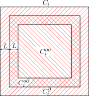
Let $C_{1}$ and $C_{2}$ be such that $C_{i}=C_{i}^{o}\cup C_{i}^{\partial}$, where $C_{i}^{o}:=\{x\in C_{i}\>|\>\mathrm{dist}\,(x,(C_{i})^{c})>L\}$, where $A^{c}$ is the complement of set $A$. With further decomposition $C_{i}^{o}=C^{oo}_{i}+C^{o\partial}_{i}$ where $C_{i}^{oo}:=\{x\in C_{i}\>|\>\mathrm{dist}\,(x,(C_{i})^{c})>2L\}$ (see Figure 2). Let $\mathcal{L}_{i}=\mathcal{L}_{i}^{o}+\mathcal{L}_{i}^{\partial}$ and $\mathcal{L}_{i}^{o}=\mathcal{L}_{i}^{oo}+\mathcal{L}_{i}^{o\partial},\;i=1,2$ be the corresponding decomposition of the generator $\mathcal{L}$, then

$$[\mathcal{L}_{1},\mathcal{L}_{2}]=[\mathcal{L}_{1}^{\partial},\mathcal{L}_{2}^{\partial}]$$

and

$$[\mathcal{L}_{1},[\mathcal{L}_{1},\mathcal{L}_{2}]]=[[\mathcal{L}_{1}^{o\partial},\mathcal{L}_{1}^{\partial}],\mathcal{L}_{2}^{\partial}]+[\mathcal{L}_{1}^{\partial},[\mathcal{L}_{1}^{\partial},\mathcal{L}_{2}^{\partial}]]\,.$$

Proof.

The proof of the first statement follows directly from Lemma 15 by observing that $\mathrm{dist}\,(C_{1}^{o},C_{2}^{o})=2L$ and

$$\mathrm{dist}\,(C_{1}^{o},C_{2}^{\partial})=\mathrm{dist}(C_{1}^{\partial},C_{2}^{o})=L\,.$$

For the second statement, using the same lemma, we compute

$$[\mathcal{L}_{1},[\mathcal{L}_{1},\mathcal{L}_{2}]]=[\mathcal{L}_{1}^{o},\mathcal{L}_{1}^{\partial}\mathcal{L}_{2}^{\partial}]-[\mathcal{L}_{1}^{o},\mathcal{L}_{2}^{\partial}\mathcal{L}_{1}^{\partial}]+[\mathcal{L}_{1}^{\partial},[\mathcal{L}_{1}^{\partial},\mathcal{L}_{2}^{\partial}]]\,.$$

The first term on the right hand side can be further simplified

$$[\mathcal{L}_{1}^{o},\mathcal{L}_{1}^{\partial}\mathcal{L}_{2}^{\partial}] =\mathcal{L}_{1}^{o}\mathcal{L}_{1}^{\partial}\mathcal{L}_{2}^{\partial}-\mathcal{L}_{1}^{\partial}\mathcal{L}_{2}^{\partial}\mathcal{L}_{1}^{o}=\mathcal{L}_{1}^{o}\mathcal{L}_{1}^{\partial}\mathcal{L}_{2}^{\partial}-\mathcal{L}_{1}^{\partial}\mathcal{L}_{1}^{o}\mathcal{L}_{2}^{\partial}$$

$$=[\mathcal{L}_{1}^{o},\mathcal{L}_{1}^{\partial}]\mathcal{L}_{2}^{\partial}=[\mathcal{L}_{1}^{oo}+\mathcal{L}_{1}^{o\partial},\mathcal{L}_{1}^{\partial}]\mathcal{L}_{2}^{\partial}$$

$$=[\mathcal{L}_{1}^{o\partial},\mathcal{L}_{1}^{\partial}]\mathcal{L}_{2}^{\partial}\,,$$

where in the second equation we used the fact that $\mathcal{L}_{2}^{\partial}\mathcal{L}_{1}^{o}=\mathcal{L}_{1}^{o}\mathcal{L}_{2}^{\partial}$ and in the last equation $[\mathcal{L}_{1}^{oo},\mathcal{L}_{1}^{\partial}]=0$. The same procedure leads to simplifying the second term but the third cannot be simplified further. Combining all these steps we obtain the result of the proposition. $\Box$

Fig. 2: Sub-lattice partitioning. Note that we use the notation $\partial C_{i}$ to denote $\bar{C}\setminus C$, see also Figure 1.

The estimation of the commutator in Theorem 10 requires local estimates on the first and second discrete derivatives of the solution to the backward Kolmogorov equation by the discrete derivatives of the initial data

Lemma 17.

The solution of the equation

$$\partial_{t}u=\mathcal{L}u\,,\;\;\;t\in(0,T]\,,\;\;\;\;u(0,\sigma)=f(\sigma)\,,$$ (35)

satisfies the bounds

$$\max_{x\in{\Lambda}_{N}}\|{\delta_{x}u(t,\cdotp)}\|_{\infty}\leq C\max_{x\in{\Lambda}_{N}}\|{\delta_{x}u(0,\cdotp)}\|_{\infty}$$ (36)

and

$$\max_{x,y\in{\Lambda}_{N}}\|\,\delta_{xy}u(t,\cdot)\,\|_{\infty}\leq C\big{[}\max_{x\in{\Lambda}_{N}}\|{\delta_{x}u(0,\cdotp)}\|_{\infty}+\max_{x,y\in{\Lambda}_{N}}\|\,\delta_{xy}u(0,\cdot)\,\|_{\infty}\big{]}\,,$$ (37)

where $C$ is a constant independent of $N$, however, it may depend exponentially on $t$.

Proof.

Using (30) and Lemma 12, we have

$$\|{\delta_{x}u(t,\cdotp)}\|_{\infty}\leq\|{\delta_{x}u(0,\cdotp)}\|_{\infty} + \mathcal{O}(1)\int_{0}^{t}\|{\delta_{x}u(s,\cdotp)}\|_{\infty}\,ds$$ (38)

$$+ \mathcal{O}(\frac{1}{L})\int_{0}^{t}\sum_{|x-y|\leq L}\|{\delta_{y}u(s,\cdotp)}\|_{\infty}\,ds\,.$$

Here the symbol $\mathcal{O}$ is asymptotic in the size of the system $N\to\infty$. Setting $\gamma(t)=\max_{x\in{\Lambda}_{N}}\|{\delta_{x}u(t,\cdotp)}\|_{\infty}$ we have

$$\|{\delta_{x}u(t,\cdotp)}\|_{\infty}\leq\gamma(0)+\mathcal{O}(1)\int_{0}^{t}\gamma(s)ds+\mathcal{O}(\frac{1}{L})L\int_{0}^{t}\gamma(s)\,ds\,,$$

or

$$\gamma(t)\leq\gamma(0)+\mathcal{O}(1)\int_{0}^{t}\gamma(s)\,ds\,.$$

Applying Gronwall’s inequality we conclude the proof and obtain the bound

$$\gamma(t)\leq e^{ct}\gamma(0)\,.$$

The inequality (37) follows similarly from (32) and from Lemma 20. $\Box$

The commutator, as shown in Lemma 16, is a localized quantity that depends only on the boundary sites of the decomposed sub-lattices. Thus the localized estimate in Lemma 17 gives us a tool in order to reveal the scaling of the commutator when acting on macroscopic observables.

5.4 Proof of Theorem 10

By Lemma 16, the commutator can be written as $[\mathcal{L}_{1}^{\partial},\mathcal{L}_{2}^{\partial}]$, which due to Lemma 15 is expanded to

$$[\mathcal{L}_{1}^{\partial},\mathcal{L}_{2}^{\partial}]u(t,\sigma)=\sum_{\begin{subarray}{c}x\in\Lambda_{1}^{\partial},y\in\Lambda_{2}^{\partial}\\ |x-y|\leq L\end{subarray}} c_{1}(x,\sigma)c_{2}(y,\sigma^{x})\delta_{y}u(\sigma^{x},t)-c_{1}(x,\sigma)c_{2}(y,\sigma)\delta_{y}u(\sigma,t)$$

$$- c_{1}(x,\sigma^{y})c_{2}(y,\sigma)\delta_{x}u(\sigma^{x},t)+c_{1}(x,\sigma)c_{2}(y,\sigma)\delta_{x}u(\sigma,t)\,.$$

On the other hand, by a straightforward calculation, we have

$$\mathcal{L}_{1}^{\partial}\mathcal{L}_{2}^{\partial}u(t,\sigma)= \sum_{\begin{subarray}{c}x\in\Lambda_{1}^{\partial},y\in\Lambda_{2}^{\partial}\\ |x-y|\leq L\end{subarray}}c_{1}(x,\sigma)c_{2}(y,\sigma^{x})\delta_{xy}u(t,\sigma)$$

$$-\sum_{\begin{subarray}{c}x\in\Lambda_{1}^{\partial},y\in\Lambda_{2}^{\partial}\\ |x-y|\leq L\end{subarray}}c_{1}(x,\sigma)\delta_{x}c_{2}(y,\sigma)\delta_{y}u(t,\sigma)\,.$$

Taking norms on both sides similarly to Lemma 11 and using the fact that the rates are bounded functions on ${\Lambda}_{N}\times\Sigma$,

$$\|{[\mathcal{L}_{1},\mathcal{L}_{2}]u(t,\cdotp)}\|_{\infty} \leq C\sum_{\begin{subarray}{c}x\in\Lambda_{1}^{\partial},y\in\Lambda_{2}^{\partial}\\ |x-y|\leq L\end{subarray}}\|{\delta_{xy}u(t,\cdotp)}\|_{\infty}+\|{\delta_{y}u(t,\cdotp)}\|_{\infty}\leq C\,,$$ (39)

where the second inequality follows from Proposition 13, using the fact that the initial data are macroscopic observables, i.e., belong to $C^{2}({{\mathcal{S}}})$. Similarly, we obtain the commutator estimate for the Strang scheme.

Next, we turn our attention to (25). Many observables are in $C^{2}({{\mathcal{S}}})$, but also satisfy the local bound (24) as one can see in Section 5.1. Under this assumption, we obtain from (39) the bound for the commutator

$$\|{[\mathcal{L}_{1},\mathcal{L}_{2}]u(t,\cdotp)}\|_{\infty}\leq C\sum_{\begin{subarray}{c}x\in\Lambda_{1}^{\partial},y\in\Lambda_{2}^{\partial}\\ |x-y|\leq L\end{subarray}}\|{\delta_{xy}u(t,\cdotp)}\|_{\infty}+\|{\delta_{y}u(t,\cdotp)}\|_{\infty}\\ \leq C\big{[}\max_{x,y\in{\Lambda}_{N}}\|{\delta_{xy}u(0,\cdotp)}\|_{\infty}+\max_{y\in{\Lambda}_{N}}\|{\delta_{y}u(0,\cdotp)}\|_{\infty}\big{]}\sum_{\begin{subarray}{c}x\in\Lambda_{1}^{\partial},y\in\Lambda_{2}^{\partial}\\ |x-y|\leq L\end{subarray}}1\,,$$ (40)

where the second inequality follows from Lemma 17. Using the fact that the initial data belong to $C^{2}({{\mathcal{S}}})$ and satisfy (24), as well as that $|C_{m}^{\partial}|=c(d)Lq^{d-1}$, where $d$ is the dimension, we deduce that

$$\|{[\mathcal{L}_{1},\mathcal{L}_{2}]u(t,\cdotp)}\|_{\infty}\leq{\frac{\tilde{C}}{N}}\sum_{\begin{subarray}{c}x\in\Lambda_{1}^{\partial},y\in\Lambda_{2}^{\partial}\\ |x-y|\leq L\end{subarray}}1\leq\frac{\tilde{C}}{N}\times M\times c(d)Lq^{d-1}\times L^{d}=C\frac{L^{d+1}}{q}\,,$$ (41)

where we used the fact that $\frac{N}{M}=Q=q^{d}$. We note that for more general, non-square lattices, the estimate is modified accordingly as the structure of neighbors in the calculation of $|C_{m}^{\partial}|$ will evidently change. Finally, the proof of (26) follows along the same lines, noting that the the summation in (41) is now replaced by summations such as

$$\sum_{\begin{subarray}{c}x\in\Lambda_{1}^{\partial},y\in\Lambda_{2}^{\partial},z\in\Lambda_{1}^{\partial}\\ |x-y|\leq L,|x-z|\leq L\end{subarray}}1\leq M\times c(d)Lq^{d-1}\times L^{d}\times L^{d}\,.$$

6 Processor communication and error analysis

In this Section we examine the balance between accuracy and processor communication in the parallel Fractional Step KMC algorithms. Our analysis is based on the local and global error analysis tools we have developed in this article.

A key feature of the fractional step methods is what we define as the Processor Communication Schedule (PCS), which dictates the order with which the hierarchy of operators in (11) are applied and for how long. For instance, for the Lie scheme (13) the processors corresponding to $\mathcal{L}_{1}$ (resp. $\mathcal{L}_{2}$) do not communicate, hence the processor communication within the algorithm occurs only each time we have to apply $e^{\Delta t\mathcal{L}_{1}}$ or $e^{\Delta t\mathcal{L}_{2}}$. For this reason, we characterize the FS-KMC algorithms (13), (14) as partially asynchronous since there is no processor communication during the period $\Delta t$. Furthermore, at every $\Delta t$ we have only local synchronization between processors, i.e., between the sets $\bar{C}_{m}\cap\bar{C}_{m^{\prime}}$ when $m\in\mathcal{I}^{1}$ and $m^{\prime}\in\mathcal{I}^{2}$. Hence, the bigger the allowable $\Delta t$ in (13) or in (14) the less processor communication we have, in which case the error in the approximation (13) or (14) worsens.

In both schemes (13), and (14), the communication schedule is fully deterministic, relying on the Trotter Theorem. On the other hand, we can construct general randomized PCS based on the Random Trotter Product Theorem, [13]. Indeed, the sub-lattice parallelization algorithm for KMC, introduced in [23], is a particular example of a fractional step algorithm with stochastic PCS. In [23, 20] each sub-lattice is selected at random, independently and advanced by KMC over a fixed time window $\Delta t$, subsequently a new random selection is made and again the sub-lattice is advanced by $\Delta t$, etc. This algorithm is easily recast as a fractional step approximation, [1].

Here we compare the deterministic and randomized PCS from the point of view of processor communication and error analysis: we specify the same error tolerance TOL for all PCS, which by means of our error analysis selects in each case a possibly different time windows $\Delta t$. Larger time windows $\Delta t$ give rise to algorithms that have less processor communication for the same error tolerance.

6.1 Randomized processor communication schedules

A generalization by Kurtz, [13], of the Trotter Theorem suggests numerically consistent schemes in which evolutions are applied not in a deterministic, prescribed, order but as a random composition of individual propagators resulting in a random evolution. Given a pure jump process $X(t)$, with stationary measure $\mu(d\xi)$, and given the infinitesimal generators $\mathcal{L}_{k}$ we define a random evolution by

$$\mathcal{T}_{n}(t)f=e^{\tau_{0}/n\mathcal{L}_{\xi_{0}}}e^{\tau_{1}/n\mathcal{L}_{\xi_{1}}}\dots e^{\tau_{N(nt)}/n\mathcal{L}_{\xi_{N(nt)}}}f\,,$$

where $N(t)$ is the number of jumps up to time $t$ and $\tau_{k}$ are the sojourn (waiting) times at the visited states $(\xi_{0},\dots,\xi_{N(t)})$. The random Trotter product theorem yields the expectation semigroup

$$\lim_{n\to\infty}\mathcal{T}_{n}(t)f=e^{t\bar{\mathcal{L}}}f\,,\;\;\;\mbox{a.s.}$$ (42)

with the generator $\bar{\mathcal{L}}$ characterized explicitly

$$\bar{\mathcal{L}}f=\int\mathcal{L}_{\xi}f\,\mu(d\xi)\,.$$ (43)

While the random Trotter formula serves as a motivation for constructing schemes in which the evolution of the system, i.e., the process $\{\sigma_{t}\}_{t\geq 0}$, is approximated by a process obtained from a random composition of propagators $e^{\Delta t\mathcal{L}_{k}}$, the error analysis in the spirit of Theorem 10 requires more careful inspection of the approximating process $\{\gamma_{kh}\}_{k=0}^{n}$ on the interval $[0,T]$ with $T=n\Delta t$.

We present the construction in a simpler case of the independent identically distributed random variables that index the individual generators $\mathcal{L}_{\xi}$. We analyze the randomized Lie scheme for the operator splitting given by $\mathcal{L}=\mathcal{L}_{1}+\mathcal{L}_{2}$. In the context of the parallel FS-KMC the random process $X(t)$ can be interpreted as a stochastic PCS. In [1] we demonstrated that the sub-lattice parallelization algorithm for KMC, introduced in [23], is a particular example of a fractional step algorithm with stochastic PCS. In [23] each sub-lattice is selected at random, independently and advanced by KMC over a fixed time window $\Delta t=h$, subsequently a new random selection is made and again the sub-lattice is advanced by $h$, etc. This algorithm is easily recast as a fractional step approximation, where we can show that $\bar{\mathcal{L}}=\frac{1}{2}\left(\mathcal{L}_{1}+\mathcal{L}_{2}\right)$ which is a time-rescaling of the original operator $\mathcal{L}$. From the numerical analysis viewpoint, our re-interpretation of the algorithm in [23] as (42) allows us to provide a rigorous justification that it is a consistent estimator of the serial KMC algorithm. Next we present the local error analysis of randomized PCS and in analogy to Lemma 6, we estimate the mean (weak) local error of the approximating $\gamma$-process.

Definition 18 (Random Lie splitting).

Let $P_{i}(t)$, $i=1,2$, be two Markov semigroups with the infinitesimal generators $\mathcal{L}_{i}$ and the transition probability kernels $p_{i}(t;\gamma,\gamma^{\prime})$. Assume $\{\xi_{1},\xi_{2},\dots\}$ be a sequence of i.i.d. Bernoulli random variables with values $\xi\in\{1,2\}$. We define the random evolution as the process $\{\gamma_{kh}\}_{k=0}^{n}$ by setting for $h>0$, $k=0,1,2,\dots,n$, and $\xi_{2k}$, $\xi_{2k-1}$ independent of $\gamma_{0},\gamma_{h},\dots,\gamma_{(k-1)h}$

$${\mathbb{E}}[f(\gamma_{kh}){\,|\,}\gamma_{(k-1)h}]:=P_{\xi_{2k-1}}(h)P_{\xi_{2k}}(h)f(\gamma_{(2k-1)h})\,,$$ (44)

where the transition probability kernel is

$$[P_{\xi_{1}}(h)P_{\xi_{2}}(h)f](\eta)=\sum_{\gamma^{\prime}}\sum_{\gamma^{\prime\prime}}p_{\xi_{1}}(h;\eta,\gamma^{\prime})p_{\xi_{2}}(h;\gamma^{\prime},\gamma^{\prime\prime})f(\gamma^{\prime\prime})\,.$$

For a given $f\in C_{b}({{\mathcal{S}}})$ we estimate the quantity ${\mathbb{E}}^{\sigma}[f(\sigma_{kh})]$ and ${\mathbb{E}}^{\gamma}[f(\gamma_{kh})]$ where the expected values are computed on the corresponding probability spaces associated with each process and conditioned on the initial states $\sigma_{0}=\sigma$ and $\gamma_{0}=\gamma$ respectively. We denote the initial states by different letters in order to distinguish between these two different probability path measures, however, the initial state is assumed to be same for both $\{\sigma_{t}\}_{t\geq 0}$ and $\{\gamma_{kh}\}_{k=0}^{n}$.

Theorem 19 (Local Error).

Assume ${\mathbb{P}\left({\xi_{k}=1}\right)}={\mathbb{P}\left({\xi_{k}=2}\right)}=\frac{1}{2}$, for the approximating process $\{\gamma_{kh}\}_{k=0}^{n}$ of Definition 18. Then for any $f\in C_{b}({{\mathcal{S}}})$ and given $\Delta t=h>0$, the exact process $\{\sigma_{t}\}_{t\geq 0}$ with $\sigma_{0}=\gamma_{0}=\gamma$ corresponding to the generator $\frac{1}{2}\mathcal{L}$ satisfies

$${\mathbb{E}}^{\gamma}[f(\gamma_{h})]-{\mathbb{E}}^{\sigma}[f(\sigma_{h})] = {\mathbb{E}}^{\xi}\left[\left(P_{\xi_{1}}(h)P_{\xi_{2}}(h)f(\gamma)-u(\gamma,h)\right)\right]$$

$$= \frac{h^{2}}{2}{\mathbb{E}}^{\xi}\left[\mathcal{L}^{2}_{\xi_{1}}+\mathcal{L}^{2}_{\xi_{2}}+2\mathcal{L}_{\xi_{1}}\mathcal{L}_{\xi_{2}}-\frac{1}{4}\mathcal{L}^{2}\right]f(\gamma)+\mathcal{O}(h^{3})\,.$$

where $u(\gamma,h)=P(h)f(\gamma)$ is the solution of the rescaled, by $1/2$, equation (6)

$$\partial_{t}u(\zeta,t)=\frac{1}{2}\mathcal{L}u(\zeta,t)\,,\quad\quad u(\zeta,0)=f(\zeta)\,.$$ (45)

Proof.

We estimate the local truncation error following similar steps as in the deterministic case. From the definition of the $\gamma$-process we have

$${\mathbb{E}}^{\gamma}[f(\gamma_{h})]={\mathbb{E}}^{\xi}[P_{\xi_{1}}(h)P_{\xi_{2}}(h)f(\gamma)]\,,$$

and similarly, using the fact that the initial states are same, $\sigma_{0}=\gamma_{0}=\gamma$,

$${\mathbb{E}}^{\sigma}[f(\sigma_{h})]=P(h)f(\gamma)=u(\gamma,h)\,.$$

Hence we obtain a representation of the mean local error

$${\mathbb{E}}^{\gamma}[f(\gamma_{h})]-{\mathbb{E}}^{\sigma}[f(\sigma_{h})]={\mathbb{E}}^{\xi}\left[\left(P_{\xi_{1}}(h)P_{\xi_{2}}(h)-P(h)\right)f(\gamma)\right]\,.$$ (46)

Now for given realizations of $\xi_{1}$, $\xi_{2}$ we have the expansion of $P_{\xi_{1}}(h)P_{\xi_{2}}(h)-P(h)$ as in the deterministic case, thus obtaining

$$[P_{\xi_{1}}(h)P_{\xi_{2}}(h)-P(h)]f=$$ (47)

$$h[\mathcal{L}_{\xi_{1}}+\mathcal{L}_{\xi_{2}}-\frac{1}{2}\mathcal{L}]f+\frac{h^{2}}{2}[\mathcal{L}^{2}_{\xi_{1}}+\mathcal{L}^{2}_{\xi_{2}}+2\mathcal{L}_{\xi_{1}}\mathcal{L}_{\xi_{2}}-\frac{1}{4}\mathcal{L}^{2}]f+\mathcal{O}(h^{3})\,.$$

Note that $\frac{1}{2}\mathcal{L}=\frac{1}{2}\mathcal{L}_{1}+\frac{1}{2}\mathcal{L}_{2}$ is associated with the process $\{\sigma_{t}\}_{t\geq 0}$. We have that the leading term of the local truncation error is ${\mathbb{E}}^{\xi}[\mathcal{L}_{\xi_{1}}+\mathcal{L}_{\xi_{2}}-\frac{1}{2}\mathcal{L}]$ and thus this term vanishes whenever $\frac{1}{2}\mathcal{L}={\mathbb{E}}^{\xi}[\mathcal{L}_{\xi_{1}}+\mathcal{L}_{\xi_{2}}]$, which holds true when $P(\xi_{k}=1)=P(\xi_{k}=2)=\frac{1}{2}$. $\Box$

Remark 6.1.

For Bernoulli variables $\xi_{i}$ with probabilities $p$ this means that the $\gamma$-process approximates a process with the generator $p\mathcal{L}_{1}+(1-p)\mathcal{L}_{2}$ instead of $\frac{1}{2}\mathcal{L}=\frac{1}{2}\mathcal{L}_{1}+\frac{1}{2}\mathcal{L}_{2}$. This indicates that the usual order of the Lie splitting is achieved by properly weighing the time steps, i.e., applying $P_{1}(h_{1})$ and $P_{2}(h_{2})$ with different time steps $h_{1}$ and $h_{2}$ respectively. This calculation also shows that if we want to obtain the generator $\mathcal{L}$ instead of $\frac{1}{2}\mathcal{L}$ in Lemma 19, then in order to evolve the process $\sigma$ by the time step $h$, each semigroup $P_{\xi_{1}},P_{\xi_{2}}$ needs to be applied with the time step $2h$, giving rise to the approximating process $\gamma_{h}$. In this case we have the local error representation

$${\mathbb{E}}^{\gamma}[f(\gamma_{h})]-{\mathbb{E}}^{\sigma}[f(\sigma_{h})]: = {\mathbb{E}}^{\xi}\left[\left(P_{\xi_{1}}(2h)P_{\xi_{2}}(2h)f(\gamma)-u(\gamma,h)\right)\right]$$

$$= \frac{h^{2}}{2}{\mathbb{E}}^{\xi}\left[4\mathcal{L}^{2}_{\xi_{1}}+4\mathcal{L}^{2}_{\xi_{2}}+8\mathcal{L}_{\xi_{1}}\mathcal{L}_{\xi_{2}}-\mathcal{L}^{2}\right]f(\gamma)$$

$$+\mathcal{O}(h^{3})\,,$$

where $u(\gamma,h)=P(h)f(\gamma)$ is the solution of (6).

6.2 Comparison of deterministic and random schedules

The presented error analysis allows us to evaluate and compare deterministic (Lie and Strang) PCS introduced in [1], as well as randomized PCS such as the one in Lemma 19, introduced earlier in [23]. We compare the deterministic and randomized PCS from the point of view of processor communication and error analysis by specifying the same error tolerance TOL for all PCS which, by means of our error analysis, selects in each case a possibly different time window $\Delta t$. Larger time windows give rise to algorithms that have less processor communication for the same error tolerance. We start with the Lie and Strang schemes.

We fix the same error tolerance level TOL in the Lie and Strang global errors (20) and (22) respectively. We also fix the same time window $T=n_{L}\Delta t_{L}$ and $T=n_{S}\Delta_{S}$ where $\Delta t_{L}$ and $\Delta t_{S}$ are the respective time steps of the Lie and the Strang schemes that will ensure the same tolerance level TOL up to time $T$. Based on Theorems 7 and 10 we have that the leading errors are governed by the commutators

$$\mathrm{TOL}\sim C_{\mathrm{Lie}}(T)\Delta t_{\mathrm{Lie}}\,,\;\quad C_{\mathrm{Lie}}(T)=\max_{k=0,\dots,n}\|\,[\mathcal{L}_{1},\mathcal{L}_{2}]u(t_{k})\,\|_{\infty}\,,$$ (49)

and

$$\mathrm{TOL} \sim C_{\mathrm{Strang}}(T)\Delta t_{\mathrm{Strang}}^{2}\,,$$ (50)

$$\quad C_{\mathrm{Strang}}(T) = \max_{k=0,\dots,n}\|\,\Bigl{(}[\mathcal{L}_{1},[\mathcal{L}_{1},\mathcal{L}_{2}]]-2[\mathcal{L}_{2},[\mathcal{L}_{2},\mathcal{L}_{1}]]\Bigr{)}u(t_{k})\,\|_{\infty}\,,$$

where $u=u(t)$ solves (6). Furthermore, due to (25) and (26) we have that

$$\mathrm{TOL}\sim\mathcal{O}\Big{(}\frac{L^{d+1}}{q}\Big{)}\Delta t_{\mathrm{Lie}}\,,\quad\mathrm{TOL}\sim\mathcal{O}(\frac{L^{2d+1}}{q}\Big{)}\Delta t_{\mathrm{Strang}}^{2}\,.$$ (51)

In the case of the randomized PCS the same reasoning as in Theorem 7 allows us to iterate the mean local error (6.1) to obtain

$$\mathrm{TOL} \sim C_{\mathrm{Random}}(T)\Delta t_{\mathrm{Random}}\,\,,$$

$$\quad C_{\mathrm{Random}}(T) =\max_{k=0,\dots,n}{\mathbb{E}}^{\xi}\left[4\mathcal{L}^{2}_{\xi_{1}}+4\mathcal{L}^{2}_{\xi_{2}}+8\mathcal{L}_{\xi_{1}}\mathcal{L}_{\xi_{2}}-\mathcal{L}^{2}\right]u(t_{k})\,,$$ (52)

where $u=u(t)$ solves (6). We now easily obtain that

$${\mathbb{E}}^{\xi}\left[4\mathcal{L}^{2}_{\xi_{1}}+4\mathcal{L}^{2}_{\xi_{2}}+8\mathcal{L}_{\xi_{1}}\mathcal{L}_{\xi_{2}}-\mathcal{L}^{2}\right]u(t)=\left[4\mathcal{L}^{2}_{1}+4\mathcal{L}^{2}_{2}+\mathcal{L}^{2}\right]u(t)\,.$$

Thus, due to the rigorous remainder bounds in Section 5 on the solution of (6) such as Lemma 13, we have that the term $\|\,\left[4\mathcal{L}^{2}_{1}+4\mathcal{L}^{2}_{2}+\mathcal{L}^{2}\right]u\,\|_{\infty}$ is of order $\mathcal{O}(1)$ in the system size $N$, and we have

$$\mathrm{TOL}\sim\mathcal{O}(1)\Delta t_{\mathrm{Random}}\,.$$ (53)

In order to achieve the same error tolerance TOL, (51) and (53) imply the following relation between the respective time steps

$$\delta t_{\mathrm{SSA}}\ll\Delta t_{\mathrm{Random}}\sim\frac{L^{d+1}}{q}\Delta t_{\mathrm{Lie}}<\Delta t_{\mathrm{Lie}}\sim L^{d}\Delta t_{\mathrm{Strang}}^{2}<\Delta t_{\mathrm{Strang}}\,.$$ (54)

Here $q$ is the diameter of each of the cells $C_{k}$ in Figure 1, and $\delta t_{\mathrm{SSA}}=\mathcal{O}(1/N)$ is the stochastic time step (the waiting time) of the SSA algorithm [7], which is exponentially distributed according to (2).

The relation (54) has several practical implications.

1. The selection of the time window $\Delta t$ in each PCS is intrinsically goal-oriented in the sense that it depends directly on the macroscopic observable $f(\sigma)$ through the commutator estimates of the solution to (6).

2. The random and deterministic PCS studied here are rigorously partially asynchronous as their respective time windows are much larger than the SSA time step $\delta t_{\mathrm{SSA}}$ for a given error tolerance.

3. The Lie scheme (13) is expected to parallelize better than the randomized PCS in [23] when $L^{d+1}\ll q$, since it allows a $q$-times larger time step $\Delta t$ for the same accuracy. This outcome is also demonstrated in Figure 3.

4. Finally, among the PCS we studied, the Strang PCS yields parallel schemes with the least processor communication, at least when $L\sim\mathcal{O}(1)$, due to its higher order accuracy and the commutator estimate (26).

Example 6.1.

We demonstrate this comparison in a computational example in which a jump process defined by Arrhenius spin-flip dynamics on a one-dimensional lattice was simulated. The simulated system corresponds to the Ising model with nearest-neighbor interactions and spins taking values in $\{0,1\}$. The rate of the process is give by

$$c(x,\sigma)=c_{d}(1-\sigma(x))+c_{a}\sigma(x)e^{-\beta U(x)}\,,$$

where $U(x)=J(\sigma(x-1)+\sigma(x+1))+\bar{h}$, and $c_{d}$, $c_{a}$, $\beta$, $J$, $h$ are the parameters of the model.

We verified the theoretical order of convergence by computing the error

$$\int_{0}^{T}|{\mathbb{E}}[C(t)]-{\mathbb{E}}[\tilde{C}(t)]|\,dt$$

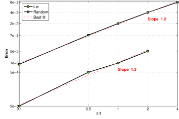
where $C(t)$ and $\tilde{C}(t)$ are the reference KMC and the FS-KMC solution, respectively, obtained by averaging the spatial mean coverage process $C(t)=\sum_{x\in{\Lambda}_{N}}\sigma_{t}(x)$ of the system over $K$ independent realizations. For the reference solution, the classical stochastic simulation algorithm (SSA) was used. In order to eliminate the impact of the statistical averaging error $K=10^{5}$ independent samples were used. The error bars are below resolution of the graph depicted in Figure 3. In Figure 3 the error behavior is compared for different values of the splitting time step $h\equiv\Delta t$ for the randomized PCS and the Lie splitting. The lattice size is $N=800$ and the parameters of the system are $\beta=15$, $J=0.37$, $h=0.5$ and $c_{a}=c_{d}=1$. For the fractional step algorithm four processors were used, thus the size of the sub-lattice is $q=100$. The final time is chosen to be $T=4$.

Fig. 3: Convergence of the weak error for deterministic and randomized Lie splitting.

Example 6.2.

In this example we investigate the dependence of the weak error, as defined in the previous example, on the sub-lattice parameter $q$. The model we used to run the simulation is Ising model, as described in Example 6.1. The parameters for the model are $\beta=5$, $J=1$, $h=0.5$, and $c_{a}=c_{d}=1$. The final time is chosen to be $T=5$ and the dimension of the lattice $N=480$. For the FS-KMC algorithm a constant, and rather large, time step parameter $\Delta t=5$ was used. For the FS-KMC algorithm we used $K=10^{4}$ samples to compute the mean value of the solution on the interval $[0,T]$ and for the reference solution, which was obtained with the SSA algorithm, $K=10^{5}$ samples were used.

Fig. 4: Dependence of the weak error on the sub-lattice size parameter $q$, see also (54).

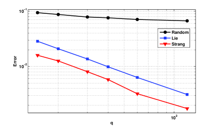
In Figure 4 we can observe that the deterministic schedules of Lie and Strang give better results than those of the random PCS. Also the Strang scheme has lower error than the Lie scheme as expected from the theoretical analysis. Finally, the dependence of the error on $\frac{1}{q}$ is also revealed, which in logarithmic scale is shown as a straight line.

7 The infinite volume limit

In this paper we considered interacting particle systems defined on a $d$-dimensional lattice ${\Lambda}_{N}$, as the numerical analysis and simulations for the parallel fractional step Kinetic Monte Carlo are performed on a finite lattice of size $N$. However, given the size of real molecular systems it is necessary that numerical estimates are independent of the system size $N$ as we showed in Section 5. Alternatively we can consider the case $N\to\infty$, e.g., by setting up our analysis on the infinite lattice $\Lambda=\mathbb{Z}^{d}$. We outline the latter approach here for completeness of our analysis. We refer to [15] for a comprehensive study of interacting particle systems set on infinite lattices.

First, we consider the configuration space ${\mathcal{S}}=\Sigma^{\Lambda}$, where $\Lambda=\mathbb{Z}^{d}$ and the space of bounded continuous functions $C_{b}({{\mathcal{S}}})$. Then the generator (7) is defined on a suitable domain $\cal D(\mathcal{L})$,

$$\mathcal{L}:D(\mathcal{L})\subset C_{b}({{\mathcal{S}}})\mapsto C_{b}({{\mathcal{S}}})\,.$$

In this case, Theorem 7 is restated similarly to Theorem 3 in [10], provided the solution $u=u(t)$ of (6) satisfies $u(t_{k})\in{\cal D}(\mathcal{L}_{1}^{m_{1}}\mathcal{L}_{2}^{m_{2}})$ for $|m|\leq 3$ and $k=0,\dots,n$. As it was also pointed out in [10] this is in principle an uncheckable hypothesis. However, this is not the case here: due to the results of Section 5 we have that if $f\in C^{2}({{\mathcal{S}}})$ is a macroscopic observable, where

$$C^{m}({{\mathcal{S}}}):=\{f\in C_{b}({{\mathcal{S}}}){\,|\,}\sum_{k=1}^{m}\|{f}\|_{k}<\infty\}\,,\forall m\in\mathbb{N}\,,$$

then $u(t)\in{\cal D}(\mathcal{L}_{1}^{m_{1}}\mathcal{L}_{2}^{m_{2}})$ due to Theorem 10 and Remark 5.1. Therefore, all estimates of Section 5 hold also true in the infinite lattice $\Lambda$, which is certainly not unexpected since all previous results in ${\Lambda}_{N}$ were independent of the system size $N$.

8 Conclusions

In this paper, we derived numerical error estimates for the Fractional Step Kinetic Monte Carlo (FS-KMC) algorithms proposed in [1] for the parallel simulation of interacting particle systems on a lattice. These algorithms have the capacity to simulate a wide range of spatio-temporal scales of spatially distributed, non-equilibrium physiochemical processes with complex chemistry and transport micro-mechanisms, while they can be tailored to specific hierarchical parallel architectures such as clusters of Graphical Processing Units. A key aspect of our approach relies on emphasizing a goal-oriented error analysis for macroscopic observables (e.g., density, energy, correlations, surface roughness), rather than focusing on strong topology estimates for individual trajectories or estimating probability distributions solving the Master Equation (Forward Kolmogorov Equation). Our analysis also addresses earlier work on parallel KMC algorithms [23, 20] that fit into the FS-KMC framework. Furthermore, moving beyond the parallelization problems discussed here, it appears that these methodologies, introduced in Section 5, can be generally useful in the development and study of numerical approximations of molecular and other extended systems. Our error analysis allows us to address systematically the processor communication of different parallelization strategies for KMC by comparing their (partial) asynchrony, which in turn is measured by their respective fractional step time-step for a prescribed error tolerance.

APPENDIX

Appendix A A general form of Gronwall’s inequality

For the sake of completeness we prove a variant of Gronwall’s lemma for a particular case that appears in the proof of Proposition 17. We prove it in the presence of two equations, but the result can be easily generalized for a system of equations.

Lemma 20 (Gronwall’s inequality).

Let $\vartheta$ and $\varphi$ satisfy the following inequalities

$$\varphi(t) \leq \varphi(0)+\int_{0}^{t}\varphi(s)\,ds$$

$$\vartheta(t) \leq \vartheta(0)+\int_{0}^{t}\vartheta(s)\,ds+\int_{0}^{t}\varphi(s)\,ds$$

then

$$\varphi(t) \leq e^{t}\varphi(0)$$ (55)

$$\vartheta(t) \leq e^{t}\vartheta(0)+(e^{t}+te^{t}-1)\varphi(0)$$ (56)

Proof.

The first estimate follows directly from Gronwall’s inequality. By integrating this inequality on $[0,t]$

$$\int_{0}^{t}\varphi(s)\leq(e^{t}-1)\varphi(0)\,,$$

and by substituting this to the second inequality we obtain

$$\vartheta(t)\leq\vartheta(0)+(e^{t}-1)\varphi(0)+\int_{0}^{t}\vartheta(s)\,ds\,.$$

If we multiply by $e^{-t}$ and integrate on $[0,t]$ we have

$$\int_{0}^{t}\Bigl{[}e^{-r}\int_{0}^{r}\vartheta(r)\Bigr{]}^{\prime}\,dr\leq(1-e^{-t})\vartheta(0)+(e^{t}+te^{t}-1)\varphi(0)\,,$$

and after straightforward calculations

$$\vartheta(t)\leq e^{t}\vartheta(0)+(e^{t}+te^{t}-1)\varphi(0)\,.$$

$\Box$

Remark A.1.

Let $\Phi(t)=(\varphi_{1}(t),\dots,\varphi_{n}(t))$ satisfying

$$\Phi(t)\leq\Phi(0)+\int_{0}^{t}A\Phi(s)\,ds$$

where $A$ is a constant lower triangular matrix and the inequality has the meaning that it is true component-wise, then

$$\Phi(t)\leq B(t)\Phi(0)\,,$$

where $B$ is a lower triangular matrix with elements exponentially depending on $t$.

References

- [1] G. Arampatzis, M. A. Katsoulakis, P. Plecháč, M. Taufer, and L. Xu, Hierarchical fractional-step approximations and parallel kinetic Monte Carlo algorithms, J. Comp. Phys., (2012), doi: 10.1016/j.jcp.2012.07.017.
- [2] S. M. Auerbach, Theory and simulation of jump dynamics, diffusion and phase equilibrium in nanopores., Int. Rev. Phys. Chem., 19 (2000).
- [3] A. B. Bortz, M. H. Kalos, and J. L. Lebowitz, A new algorithm for Monte Carlo simulation of Ising spin systems, J. Comp. Phys., 17 (1975), pp. 10–18.
- [4] A. Chatterjee and D. G. Vlachos, An overview of spatial microscopic and accelerated kinetic Monte Carlo methods, J. Comput.-Aided Mater. Design, 14 (2007), pp. 253–308.
- [5] S. G. Eick, A. G. Greenberg, B. D. Lubachevsky, and A. Weiss, Synchronous relaxation for parallel simulations with applications to circuit-switched networks, ACM Trans. Model. Comput. Simul., 3 (1993), pp. 287–314.
- [6] Crispin Gardiner, Handbook of Stochastic Methods: for Physics, Chemistry and the Natural Sciences, Springer, 4th ed., 2009.
- [7] D. T. Gillespie, A general method for numerically simulating the stochastic time evolution of coupled chemical reactions, J. of Comp. Phys., 22 (1976), pp. 403–434.
- [8] Ernst Hairer, Christian Lubich, and Gerhard Wanner, Geometric numerical integration, vol. 31 of Springer Series in Computational Mathematics, Springer-Verlag, Berlin, second ed., 2006. Structure-preserving algorithms for ordinary differential equations.
- [9] P. Heidelberger and D. M. Nicol, Conservative parallel simulation of continuous time markov chains using uniformization, IEEE Trans. Parallel Distrib. Syst., 4 (1993), pp. 906–921.
- [10] T. Jahnke and D. Altıntan, Efficient simulation of discrete stochastic reaction systems with a splitting method, BIT, 50 (2010), pp. 797–822.
- [11] C. Kipnis and C. Landim, Scaling Limits of Interacting Particle Systems, Springer-Verlag, 1999.
- [12] G. Korniss, M. A. Novotny, and P. A. Rikvold, Parallelization of a dynamic Monte Carlo algorithm: A partially rejection-free conservative approach, J. Comp. Phys., 153 (1999), pp. 488–508.
- [13] T. G. Kurtz, A random Trotter product formula, Proc. Amer. Math. Soc., 35 (1972), pp. 147–154.
- [14] D. P. Landau and K. Binder, A Guide to Monte Carlo Simulations in Statistical Physics, Cambridge University Press, Cambridge, 2000.
- [15] Thomas M. Liggett, Interacting Particle Systems, vol. 276 of Grundlehren der mathematischen Wissenschaften, Springer-Verlag, New York, Berlin, Heidelberg, Tokyo, 1985.
- [16] Da-Jiang Liu and J. W. Evans, Atomistic and multiscale modeling of CO-oxidation on Pd(100) and Rh(100): From nanoscale fluctuations to mesoscale reaction fronts, Surf. Science, 603 (2009), pp. 1706–1716.
- [17] B. D. Lubachevsky, Efficient parallel simulations of dynamic Ising spin systems, J. Comput. Phys., 75 (1988), pp. 103–122.
- [18] M. Merrick and K. A. Fichthorn, Synchronous relaxation algorithm for parallel kinetic Monte Carlo simulations of thin film growth, Phys. Rev. E, 75 (2007), p. 011606.
- [19] G. Nandipati, Y. Shim, J. G. Amar, A. Karim, A. Kara, T. S. Rahman, and O. Trushin, Parallel kinetic Monte Carlo simulations of Ag(111) island coarsening using a large database, Journal of Physics Condensed Matter, 21 (2009), p. 084214.
- [20] S. Plimpton, C. Battaile, M. Chandross, L. Holm, A. Thompson, V. Tikare, G. Wagner, E. Webb, X. Zhou, C. Garcia Cardona, and A. Slepoy, Crossing the Mesoscale No-Man’s Land via Parallel Kinetic Monte Carlo, Tech. Report SAND2009-6226, Sandia National Laboratory, 2009.
- [21] K Reuter, D Frenkel, and M Scheffler, The steady state of heterogeneous catalysis, studied by first-principles statistical mechanics, Physical Review Letters, 93 (2004).
- [22] Y. Shim and J. G. Amar, Rigorous synchronous relaxation algorithm for parallel kinetic Monte Carlo simulations of thin film growth, Phys. Rev. B, 71 (2005), p. 115436.
- [23] , Semirigorous synchronous relaxation algorithm for parallel kinetic Monte Carlo simulations of thin film growth, Phys. Rev. B, 71 (2005), p. 125432.
- [24] G. Szabo and G. Fath, Evolutionary games on graphs, Physics Reports, 446 (2007), pp. 97–216.
- [25] H. F. Trotter, On the product of semi-groups of operators, Proc. Amer. Math. Soc., 10 (1959), pp. 545–551.