Resilience of the Spectral Standard Model

Abstract

We show that the inconsistency between the spectral Standard Model and the experimental value of the Higgs mass is resolved by the presence of a real scalar field strongly coupled to the Higgs field. This scalar field was already present in the spectral model and we wrongly neglected it in our previous computations. It was shown recently by several authors, independently of the spectral approach, that such a strongly coupled scalar field stabilizes the Standard Model up to unification scale in spite of the low value of the Higgs mass. In this letter we show that the noncommutative neutral singlet modifies substantially the RG analysis, invalidates our previous prediction of Higgs mass in the range 160–180 Gev, and restores the consistency of the noncommutative geometric model with the low Higgs mass.

year number number identifier

I Introduction

The noncommutative geometry framework representing space-time as a product of a continuous four-dimensional manifold by a finite discrete space has provided a geometric explanation Why for the intricate complexity of the standard model of particle physics coupled to gravity, including all its fine features such as the full Higgs sector whose geometric origin then becomes obvious. Despite the many successes of this noncommutative model, one of its predictions coming from using the spectral action at unification scale concerning the Higgs mass, turns out to be contradicted by recent experimental results. At some time, it was indeed claimed that the Higgs mass must lie in the range of $160$ to $180$ Gev. Now that experimental evidence shows that the Higgs mass is of the order of $125$ GeV, there are two difficulties that the spectral model needs to resolve in order to survive as a model of gravity unified with the Standard model in its actual experimentally validated form. The above discrepancy between $125$ and $160-180$ Gev could be brushed away due to the enormous extrapolation involved in running down from unification scale of $10^{17}$ Gev to the electroweak scale, arguing that the order of magnitude of the mass is correct while getting the precise value was too much to ask. But a second difficulty is much more problematic: since such a low mass of the Higgs creates an instability in the Higgs potential (where the quartic coupling of the Higgs becomes negative at high energy) thus ruling out the “big desert” hypothesis which we were using, and invalidating the positivity of the coupling at unification which is an essential prediction of the spectral action.

The main result of this paper is that the full spectral action as computed in our previous paper framework , published in 2010, in fact already contains the solution to this second difficulty and at the same time shows the compatibility of the spectral model with the above low experimental Higgs mass. The fact is that in our previous prediction of the Higgs mass, we assumed, incorrectly, that the additional real singlet field $\sigma$ responsible for the neutrino Majorana masses framework would not interfere much with the Higgs mass prediction and could be ignored. We became aware of the non-trivial role played by such a scalar field when we realized that it has the same structure of couplings as in the papers by various authors Elias1 , Elias2 , Darkon , lebedev , Bezr who proposed to solve the above instability problem of the Standard Model precisely by adding a new scalar field strongly coupled to the Higgs. Their result shows that, adding this new scalar field, everything would be fine, with a Higgs of 125 Gev, for SM at high energies. It turns out that by miracle their proposed couplings are exactly the same as the ones which were delivered before by the spectral action in framework .

II Higgs-Singlet scalar potential

The spectral action for Standard Model was calculated for a cutoff function starting with the Dirac operator of the corresponding noncommutative space, using heat kernel methods. The part involving the Higgs and singlet fields is given by framework

$$-\frac{2}{\pi^{2}}f_{2}\Lambda^{2}{\displaystyle\int}d^{4}x\sqrt{g}\left(\frac{1}{2}a\overline{H}H+\frac{1}{4}c\,\sigma^{2}\right)$$

$$+\frac{1}{2\pi^{2}}f_{0}{\displaystyle\int}d^{4}x\sqrt{g}\left(b\left(\overline{H}H\right)^{2}+a\left|\nabla_{\mu}H_{a}\right|^{2}+2e\overline{H}H\,\sigma^{2}+\frac{1}{2}d\,\sigma^{4}+\frac{1}{2}c\left(\partial_{\mu}\sigma\right)^{2}\right)$$ (1)

where $H$ is the Higgs doublet and $\sigma$ the real scalar singlet associated with the Majorana mass of the right-handed neutrino. The coefficients $f_{0}$ and $f_{2}$ are related to the spectral function by the relations $f_{0}=f\left(0\right)$ and $f_{2}={\displaystyle\int_{0}^{\infty}}f\left(u\right)du.$ The coefficients $a,b,c,d$ and $e$ are related to the fermionic Yukawa couplings and Majorana mass matrix. To simplify the analysis, we shall work in the rough approximation where the Yukawa couplings of the top quark $k^{u}$ and the neutrino (both Dirac $k^{\nu}$ and Majorana $k^{\nu_{R}}$ ) are dominant and in addition we introduce the dimensionless constant $n$ defined by the relation

$$k^{\nu}=\sqrt{n}\,k^{u}$$ (2)

In this approximation we have

$$a =\left|k^{u}\right|^{2}(n+3)$$ (3)

$$b =\left|k^{u}\right|^{4}(n^{2}+3)$$ (4)

$$c =\left|k^{\nu_{R}}\right|^{2}$$ (5)

$$d =\left|k^{\nu_{R}}\right|^{4}$$ (6)

$$e =n\left|k^{\nu_{R}}\right|^{2}\left|k^{u}\right|^{2}$$ (7)

It should be clear that there is some remaining flexibility especially in the Majorana matrix $k^{\nu_{R}}$ for the general treatment involving in full the three families of fermions. We work in the unitary gauge where three scalars of the complex Higgs doublet $H$ are gauged away allowing us to set the field $H=\left(\begin{array}[c]{c}0\\ h\end{array}\right)$ where $h$ is real. It is more transparent to work with the rescaled fields

$$\overline{h}=\left|k^{u}\right|h,\qquad\overline{\sigma}=\left|k^{\nu_{R}}\right|\sigma$$ (8)

so that the action for scalar fields reduces to the form

$$-\frac{2}{\pi^{2}}f_{2}\Lambda^{2}{\displaystyle\int}d^{4}x\sqrt{g}\left(\frac{1}{2}\left(n+3\right)\overline{h}^{2}+\frac{1}{4}\overline{\sigma}^{2}\right)$$

$$+\frac{1}{2\pi^{2}}f_{0}{\displaystyle\int}d^{4}x\sqrt{g}\left(\left(n^{2}+3\right)\overline{h}^{4}+\left(n+3\right)\left(\partial_{\mu}\overline{h}\right)^{2}+2n\overline{h}^{2}\,\overline{\sigma}^{2}+\frac{1}{2}\,\overline{\sigma}^{4}+\frac{1}{2}\left(\partial_{\mu}\overline{\sigma}\right)^{2}\right)$$ (9)

The gauge fields kinetic terms are normalized by setting the coefficient $f_{0}$ to be $\frac{f_{0}}{2\pi^{2}}=\frac{1}{4g^{2}}.$ The scalar fields kinetic terms are then normalized by rescaling

$$\overline{h} \rightarrow\overline{h}\sqrt{\frac{2}{n+3}}g$$ (10)

$$\overline{\sigma} \rightarrow 2\overline{\sigma}g$$ (11)

so that the Higgs-singlet potential reduces to

$$V=\frac{1}{4}\left(\lambda_{h}\overline{h}^{4}+2\lambda_{h\sigma}\overline{h}^{2}\overline{\sigma}^{2}+\lambda_{\sigma}\overline{\sigma}^{4}\right)-\frac{2g^{2}}{\pi^{2}}f_{2}\Lambda^{2}\left(\overline{h}^{2}+\ \overline{\sigma}^{2}\right)$$ (12)

where

$$\lambda_{h} =\frac{n^{2}+3}{\left(n+3\right)^{2}}\left(4g^{2}\right)$$ (13)

$$\lambda_{h\sigma} =\frac{2n}{n+3}\left(4g^{2}\right)$$ (14)

$$\lambda_{\sigma} =2\left(4g^{2}\right)$$ (15)

The singlet has a strong coupling $\lambda_{\sigma}=$ $8g^{2}.$ The coupling $\lambda_{h\sigma}$ vanishes for $n=0$ and increases to $8g^{2}$ as $n\rightarrow\infty$. The coupling $\lambda_{h}$ decreases from $\frac{4}{3}g^{2}$ to $g^{2}$ for $n$ varying from $0$ to $1$ and increases again to $4g^{2}$ for $n\rightarrow\infty$.

III Running the initial conditions for the model with cutoff function

Writing the RG equations for the top quark, neutrino, Higgs and singlet quartic couplings we have RGEsing

$$\frac{dk^{t}}{dt} =\frac{k^{t}}{32\pi^{2}}\left(-\left(\frac{17}{6}g_{1}^{2}+\frac{9}{2}g_{2}^{2}+16g_{3}^{2}\right)+9\left(k^{t}\right)^{2}+2\left(k^{\nu}\right)^{2}\right)$$ (16)

$$\frac{dk^{\nu}}{dt} =\frac{k^{\nu}}{32\pi^{2}}\left(-\left(\frac{3}{2}g_{1}^{2}+\frac{9}{2}g_{2}^{2}\right)+6\left(k^{t}\right)^{2}+5\left(k^{\nu}\right)^{2}\right)$$ (17)

$$\frac{d\lambda_{h}}{dt} =\frac{1}{16\pi^{2}}\left(\left(12\left(k^{t}\right)^{2}+4\left(k^{\nu}\right)^{2}-\left(3g_{1}^{2}+9g_{2}^{2}\right)\right)\lambda_{h}\right.$$

$$\qquad\left.+2\left(12\lambda_{h}^{2}+\lambda_{h\sigma}^{2}+\frac{3}{16}\left(g_{1}^{4}+2g_{1}^{2}g_{2}^{2}+3g_{2}^{4}\right)-3\left(k^{t}\right)^{4}-\left(k^{\nu}\right)^{4}\right)\right)$$ (18)

$$\frac{d\lambda_{h\sigma}}{dt} =\frac{\lambda_{h\sigma}}{16\pi^{2}}\left(\frac{1}{2}\left(12\left(k^{t}\right)^{2}+4\left(k^{\nu}\right)^{2}-3g_{1}^{2}-9g_{2}^{2}\right)+4\left(3\lambda_{h}+\frac{3}{2}\lambda_{\sigma}+2\lambda_{h\sigma}\right)\right)$$ (19)

$$\frac{d\lambda_{\sigma}}{dt} =\frac{1}{16\pi^{2}}\left(8\lambda_{h\sigma}^{2}+18\lambda_{\sigma}^{2}\right)$$ (20)

To run these equations, we have to run first the gauge couplings $\alpha_{1},\alpha_{2}$ and $\alpha_{3}$

$${\beta_{g_{i}}=(4\pi)^{-2}\,b_{i}\,g_{i}^{3},\ \ \ {\hbox{ with }}\ \ b=(\frac{41}{6},-\frac{19}{6},-7),}$$

so that the inverse couplings are linear functions of $u=\log\,\frac{\Lambda}{M_{Z}}$ as follows

$$\alpha_{1}^{-1}(\Lambda) =\,\alpha_{1}^{-1}(M_{Z})-\frac{41}{12\pi}\,\log\,\frac{\Lambda}{M_{Z}}$$

$$\alpha_{2}^{-1}(\Lambda) =\,\alpha_{2}^{-1}(M_{Z})+\frac{19}{12\pi}\,\log\,\frac{\Lambda}{M_{Z}}$$

$$\alpha_{3}^{-1}(\Lambda) =\,\alpha_{3}^{-1}(M_{Z})+\frac{42}{12\pi}\,\log\,\frac{\Lambda}{M_{Z}}$$

where $M_{Z}$ is the mass of the $Z^{0}$ vector boson.

It is known that the predicted unification of the coupling constants does not hold exactly. The non meeting of the three gauge couplings, to within few percents, is an indication that there is some missing ingredient in our considerations, which may be related to the use of the cutoff function in the asymptotic heat kernel expansion of the spectral action ali . There are some indications that a slight deviation from the cutoff function would alter the relation

$$\frac{5}{3}g_{1}^{2}=g_{2}^{2}=g_{3}^{2}$$ (21)

which gets modified to depend on the slope of the derivative of the spectral function. We will not pursue this issue in what follows, and assume that there is some uncertainty in the actual value of the unification scale, so that the variable $u_{\rm unif}=\log\,\frac{\Lambda_{\rm unif}}{M_{Z}}$ will be tested in the range $(25,35)$ corresponding to unification scale $s$ in the range $m_{Z}e^{25}\sim 6.55245\times 10^{12}GeV$ to $m_{Z}e^{35}\sim 1.44327\times 10^{17}GeV$.

The RG equations are run down with initial conditions at unification scale for the top quark coupling $k^{t},$ the neutrino coupling $k^{\nu}=\sqrt{n}\,k^{t}$, the gauge couplings, and the quartic scalar couplings as prescribed by equations (13), (14), (15).

The effective top quark Yukawa coupling is given at unification scale by (compare with mc2 )

$$k^{t}(u_{\rm unif})=\sqrt{\frac{4}{n+3}}g$$ (22)

so the top quark mass at low scale is

$$m_{t}\left(M_{Z}\right)=k^{t}\left(0\right)\frac{246}{\sqrt{2}}=173.94\,k^{t}\left(0\right)\text{ Gev}$$ (23)

which should be compared to the experimental value which is reached for $k^{t}\left(M_{Z}\right)=0.99.$

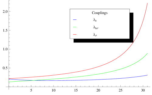
Figure 1: Running of the three parameters $\lambda_{h},$ $\lambda_{h\sigma}$ and $\lambda_{\sigma}$

We know that the quartic couplings $\lambda_{h},$ $\lambda_{h\sigma}$ and $\lambda_{\sigma}$ all run, and since they are dimensionless we can trust their running and obtain their value at low scale ($u=0$) from the initial condition at unification scale $u_{\rm unif}$. On the other hand, the mass terms give quadratic divergences, and their running cannot be trusted. We write the potential in the form

$$V=-\frac{1}{2}\left(\mu^{2}\overline{h}^{2}+\nu^{2}\overline{\sigma}^{2}\right)+\frac{1}{4}\left(\overline{h}^{4}\lambda_{h}+2\overline{h}^{2}\overline{\sigma}^{2}\lambda_{\text{h$\sigma$}}+\overline{\sigma}^{4}\lambda_{\sigma}\right)$$ (24)

The minimum is obtained for $\left\langle\overline{h}^{2}\right\rangle=\overline{v}^{2}$, $\left\langle\overline{\sigma}^{2}\right\rangle=\overline{w}^{2}$ where

$$-\mu^{2}+\bar{v}^{2}\lambda_{h}+\bar{w}^{2}\lambda_{\text{h$\sigma$}}=0,\ \ -\nu^{2}+\bar{v}^{2}\lambda_{\text{h$\sigma$}}+\bar{w}^{2}\lambda_{\sigma}=0.$$ (25)

We determine the mass terms $\mu^{2}$ and $\nu^{2}$ at low scale using this equation so that $\overline{v}^{2}$ is of order $10^{2}$ Gev and $\overline{w}^{2}$ is of order $10^{11}$ Gev. We will not worry about this fine tuning, which is related to the problem of quadratic divergencies, but note that the dilaton field scale which replaces the scale $\Lambda$ could be used to technically solve this problem as it connects the different subalgebras of the discrete space. We use the approximation $\overline{v}^{2}\ll\overline{w}^{2}$ which is also made use of to get the see-saw mechanism. To find the masses, we expand the scalar fields around the vev’s

$$\overline{h}=\overline{v}+\overline{\phi},\qquad\overline{\sigma}=\overline{w}+\overline{\tau}$$ (26)

and use (25) to expand the potential (24) up to terms of third order in $\bar{\phi}$, $\bar{\tau}$ as

$$V\sim\left(-\frac{1}{4}\bar{v}^{4}\lambda_{h}-\frac{1}{2}\bar{v}^{2}\bar{w}^{2}\lambda_{\text{h$\sigma$}}-\frac{1}{4}\bar{w}^{4}\lambda_{\sigma}\right)+\bar{v}^{2}\bar{\phi}^{2}\lambda_{h}+2\bar{v}\bar{w}\bar{\tau}\bar{\phi}\lambda_{\text{h$\sigma$}}+\bar{w}^{2}\bar{\tau}^{2}\lambda_{\sigma}$$ (27)

This expansion gives the mass terms for the fields $\overline{\phi}$ and $\overline{\tau}$ in the form of the mass matrix

$$\frac{1}{2}\left(\begin{array}[c]{cc}\overline{\phi}&\overline{\tau}\end{array}\right)M^{2}\left(\begin{array}[c]{c}\overline{\phi}\\ \overline{\tau}\end{array}\right)$$ (28)

where

$$M^{2}=2\left(\begin{array}[c]{cc}\lambda_{h}\overline{v}^{2}&\lambda_{h\sigma}\overline{v}\overline{w}\\ \lambda_{h\sigma}\overline{v}\overline{w}&\lambda_{\sigma}\overline{w}^{2}\end{array}\right)$$ (29)

The eigenvalues of the mass matrix are

$$m_{\pm}^{2}=\lambda_{h}\overline{v}^{2}+\lambda_{\sigma}\overline{w}^{2}\pm\sqrt{\left(\lambda_{h}\overline{v}^{2}-\lambda_{\sigma}\overline{w}^{2}\right)^{2}+4\lambda_{h\sigma}^{2}\overline{v}^{2}\overline{w}^{2}}$$ (30)

With the approximation $\overline{v}^{2}\ll\overline{w}^{2}$ we have

$$m_{+}^{2} \simeq 2\lambda_{\sigma}\overline{w}^{2}+2\frac{\lambda_{h\sigma}^{2}}{\lambda_{\sigma}}\overline{v}^{2}$$ (31)

$$m_{-}^{2} \simeq 2\lambda_{h}\overline{v}^{2}\left(1-\frac{\lambda_{h\sigma}^{2}}{\lambda_{h}\lambda_{\sigma}}\right)$$ (32)

Thus the Higgs mass is reduced by a factor of $\sqrt{\left(1-\frac{\lambda_{h\sigma}^{2}}{\lambda_{h}\lambda_{\sigma}}\right)}.$ This factor will be of the order $.78$ (at low scale) as shown in Figure 3.

The condition to have a stable Higgs mass at $125$ Gev is that the determinant of the mass matrix is positive

$$\lambda_{h\sigma}^{2}<\lambda_{h}\lambda_{\sigma}$$ (33)

and we check numerically that it holds at low scale as can be seen in Figure 3. The physical states are mixtures of the fields $h$ and $\sigma$ but with very small mixing of order of $\frac{\overline{v}}{\overline{w}}=\mathrm{O}\left(10^{-9}\right).$

Thus, we vary the parameter $n$ and the unification scale $u_{\rm unif}$. The physical masses of the top and Higgs fields are then determined from the values of the couplings at low energies (for $u=0$) by the formulas

$$m_{t}\left(0\right) =k^{t}\left(0\right)\frac{246}{\sqrt{2}}$$ (34)

$$m_{h}\left(0\right) =246\sqrt{2\lambda_{h}\left(0\right)\left(1-\frac{\lambda_{h\sigma}^{2}(0)}{\lambda_{h}(0)\lambda_{\sigma}(0)}\right)}$$ (35)

Numerical studies of this system of one loop RG equations in the parameter space $(n,u)$ reveal that a Higgs mass of around 125.5 Gev is reached on an almost straight curve as shown as the thick dotted line in Figure 2. This shows that one can find a suitable value $n(u)$ of the free parameter $n$ for any unification scale $u$ in the range $u\in(25,35)$ (which corresponds to the interval $6.5\times 10^{12}-1.4\times 10^{17}GeV$) such that the Higgs mass has the correct experimental value. We thus obtain a one parameter family, parameterized by $u\in(25,35)$ of consistent theories. One can check numerically that for all of them the three couplings $\lambda_{h}$, $\lambda_{h\sigma}$, $\lambda_{\sigma}$ remain positive in the running from the unification scale to the low scale and that moreover the inequality (33) holds at low scale (Figure 3).

The numerical study also shows that the top quark mass obtained is a few percents lower than the experimental value. It is known, however, for the two loop equations of the standard model, without the singlet, that at the two loop level the quartic Higgs coupling gets a very small correction, while the top quark gets a sizable correction which is 16% of the one loop QCD corrections, which are not negligible, and which pushes the top quark mass to be higher at low energies Elias2 , Zoller . We thus expect, once the two loop RG equations are worked out in the presence of a singlet, to improve the agreement of our theory with the experimental values for both the top quark mass and the Higgs mass.

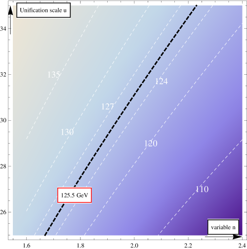
Figure 2: Higgs mass as a function of $n$ and of the unification scale $u\in(25,35)$, the thick doted line is where $m_{H}=125.5$ Gev. The thin dotted lines correspond to constant values of $m_{H}$ as indicated.

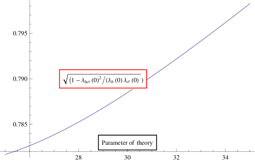
Figure 3: Correction factor at scale $u=0$ as a function of the parameter of the theory

IV Conclusions

Now that the Brout-Englert-Higgs HiggsBoson field has been discovered experimentally, it begs for a conceptual explanation of the Lagrangian of the Standard Model coupled to gravity, which would unify its juxtaposed fragmented pieces. The spectral model provides such an explanation based on two ingredients:

• An extension of the geometric paradigm treating the continuum and the discrete on the same footing.

• A principle of utmost simplicity, the spectral action principle, asserting that the action functional is a spectral function of the line element.

The model of space-time given by the product of a continuous four dimensional manifold times a noncommutative discrete space has many advantages. It allowed us to obtain the Standard Model with the correct representation for the $16$ fermions, the correct gauge fields and a Higgs doublet associated with the discrete dimension, thus providing a geometric origin for the Higgs field as a gauge field associated to the finite space. While in the first stage of development of the model, the finite space was introduced by hand, we later classified Why these finite spaces. We found that there are severe restrictions on its form, singling out, almost uniquely, the symmetries of the standard model Why . A classification of finite spaces consistent with the axioms of noncommutative geometry and which avoids the fermion doubling problem in Euclidean spaces showed that the dimension of the Hilbert space of Fermions is the square of an even integer. Among very few choices for the lowest dimensional case we obtained the algebra $\mathcal{A}=M_{2}(\mathbb{H})\oplus M_{4}(\mathbb{C})$ where $\mathbb{H}$ is the skew field of quaternions. This determines the number of fermions to be $4^{2}=16$, and thus confirms the existence of the right-handed neutrino. In addition to the Higgs field, there exists a neutral singlet field, whose vev gives Majorana mass to the right-handed neutrino. The existence of the singlet is responsible for the breakdown of the symmetry of the discrete space from $\mathbb{H\oplus H}\oplus M_{4}\left(\mathbb{C}\right)$ to $\mathbb{C\oplus H}\oplus M_{3}\left(\mathbb{C}\right)$ and thus plays a central role. The noncommutative approach predicts all the fermionic and bosonic spectrum of the standard model, and the correct representations. One can also take as a prediction that there are no other particles to be discovered, except for the three scalar fields: the Higgs field, the singlet field and the dilaton field scale . The dynamics of the fields are governed by the interactions obtained from the spectral action principle, which is based on using a function of the Dirac operator defining the metric of the noncommutative space. Despite the many successes of the noncommutative model, one of the predictions concerning the Higgs mass turned out to be problematic. At some time, it was claimed that the Higgs mass must lie in the range of $160$ to $180$ Gev. This claim was made under the assumption that the singlet field was integrated out, and replaced by its vev. This assumption turns out to be simplistic. In fact the singlet responsible for the right-handed neutrino mass gets mixed in a non-trivial way with the Higgs field. The potential was derived and given in full detail in our earlier work framework . Recently and in more than one work Elias1 , Elias2 , Darkon , lebedev , it was shown that adding a singlet (real or complex) scalar field, whose potential mixes with the Higgs field, has important consequences. It turned out that the RG equations of the combined Higgs-singlet system solves the stabilization problem faced with a light Higgs field of the order of $125$ Gev avoiding making the Higgs quartic coupling negative at very high energies. Remarkably, the form of the Higgs-singlet potential proposed recently agree with the one we derived before from the spectral action framework . The quartic couplings are determined at unification scale in terms of the gauge and Yukawa couplings. Running these relations down with the scale, give values consistent with the present data for the Higgs and top quark mass.

In this note we have analyzed the Higgs-singlet potential resulting from the spectral action with a cutoff function. We have shown that the quartic Higgs couplings of the Higgs doublet and singlet get mixed, resulting in shifting the masses of these two fields. One field, mostly composed of the Higgs get shifted down, and the one mostly made of sigma get shifted up. We have shown that it is possible to have a choice of initial conditions, consistent with the low value of around $125$ Gev for the Higgs mass and $170$ Gev for the top quark mass.

The lesson we learned from this analysis is that we have to take all the fields of the noncommutative spectral model seriously, without making assumptions not backed up by valid analysis, especially because of the almost uniqueness of the Standard Model in the noncommutative setting. In this respect this should motivate us to address the remaining questions in the noncommutative Standard Model. In particular it is important to resolve the issue of providing a way to make the three gauge couplings meet at some unification scale. There are other important questions to study in order to provide a geometric framework for the Yukawa couplings for all fermions, as well as an explanation for the number of families.

V Acknowledgments

A. H. C. is supported in part by the National Science Foundation under Grant No. Phys-0854779.

References

- (1) Ali H. Chamseddine and Alain Connes, Why the Standard Model, J. Geom. Phys. 58 (2008) 38-47.
- (2) Ali H. Chamseddine and Alain Connes, Noncommutative Geometry as a Framework for Unification of all Fundamental Interactions including Gravity. Part I, Fortsch. Phys. 58 (2010) 553-600.
- (3) J. Elias-Miro, J. Espinosa, G. Guidice, H. M. Lee and A. Sturmia, Stabilization of the Electroweak Vacuum by a Scalar Threshold effect, JHEP 1206 (2012) 031.
- (4) G. Degrassi, S. Di Vita, J. Elias-Miro, J. Espinosa, G. Guidice, G. Isidori and A. Sturmia, Higgs mass and Vacuum Stability in the Standard Model at NNLO arXiv:1205.6497.
- (5) Chian-Shu Chen and Yong Tang, Vacuum Stability, Neutrinos and Dark matter JHEP 1204 (2012) 019.
- (6) Oleg Lebedev On Stability of the Higgs Potential and the Higgs Portal, JHEP, arXiv:1203.0156.
- (7) F. Bezrukov, M. Y. .Kalmykov, B. A. Kniehl and M. Shaposhnikov, arXiv:1205.2893 [hep-ph].
- (8) M. Gonderinger, Y. Li, H. Patel and M. J. Ramsey-Musolf, JHEP 1001 (2010) 053 [hep-ph/0910.3167]; O. Lebedev and H. M. Lee, Eur. Phys. J. C 71 (2011) 1821 [hep-ph/1105.2284]; M. Kadastik, K. Kannike, A. Racioppi and M. Raidal, [hep-ph/1112.3647]; M. Gonderinger, H. Lim and M. J. Ramsey-Musolf, [hep-ph/1202.1316]; C. -S. Chen and Y. Tang [hep-ph/1202.5717].
- (9) A. Chamseddine, A. Connes, M. Marcolli, Gravity and the standard model with neutrino mixing, Adv. Theor. Math. 11 (2007) 991-1090.
- (10) Ali H. Chamseddine, Noncommutative Geometry as the key to unlock secrets of space-time, Published in Quanta of Math, editors E. Blanchard et al, Clay Mathematics Institute/AMS publication, 2010, arXiv:0901.0577.
- (11) K. Chetyrkin and M. Zoller, Three loop beta functions for the top Yukawa and the Higgs self interactions in the Standard Model, arXiv:1205.2892.
- (12) Ali H. Chamseddine and Alain Connes, Scale invariance in the spectral action, J. Math. Phys. 47 (2006) 063504.
- (13) F. Englert and R. Brout, Phys. Rev. Lett. 13, 321 (1964); P. W. Higgs, Phys. Lett. 12, 132 (1964). Phys. Rev. Lett. 13, 508 (1964); G. S. Guralnik, C. R. Hagen and T. W. B. Kibble, Phys. Rev. Lett. 13, 585 (1964).