Simulating Interference and Diffraction in Instructional Laboratories

Abstract

Studies have shown that standard lectures and instructional laboratory experiments are not effective at teaching interference and diffraction. In response, the author created an interactive computer program that simulates interference and diffraction effects using the Finite Difference Time Domain method. The software allows students to easily control, visualize, and quantitatively measure the effects. Students collected data from simulations as part of their laboratory exercise, and they performed well on a subsequent quiz—showing promise for this approach.

I Introduction

Often, interference and diffraction is taught by showing the mathematics in lecture and then performing laser interference and diffraction experiments in an instructional laboratory. However, studies show this teaching method is lacking.

Consider the following problem (see Figure 1), which should be straightforward for a student who understands the concepts. Two point sources, $2.5$ wavelengths ($\lambda$) apart, generate waves in phase. Is there constructive interference, destructive interference, or neither at points A, B, and C?

A University of Washington study asked this and other questions to $\approx 1200$ undergraduates in their standard, calculus-based, introductory physics course. Only $\approx 35\%$ answered correctly for both points A and B, and only $\approx 5\%$ answered correctly for point C. Graduate students also performed poorly; only $\approx 25\%$ answered correctly for point C.wosilait:S5 These mistakes were primarily due to fundamental misunderstandings; post-quiz student interviews included responses like, “I suppose that $2.5\lambda$ [the slit separation] is small compared to $400\lambda$ and $300\lambda$, so the sources here act like a single source.”ambrose:146 Moreover, the typical instruction method did not help; the scores for point C before and after lecture and laboratory were basically unchanged.ambrose:146 ; wosilait:S5

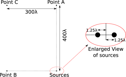
Figure 1: The diagram for the interference quiz.

Part of the problem is that light’s wave nature is only visible indirectly—though effects like interference and diffraction. Light’s peaks and valleys cannot be viewed directly. Hands-on experience seeing and controlling the waves’ interactions is useful for student understanding, so a better wave medium is needed. Ripple tanks provide this, but there are significant trade-offs between easy of use, cost, and measurement accuracy.

For example, Wosilait et al. provided students with simple ripple tanks—pans, dowels, and sponges. They are cheap and easy to use but do not allow quantitative measurements. Still, they proved effective as part of an intensive tutorial system that raised scores for point C to $\approx 45\%$.wosilait:S5

Measurements can be performed with a ripple tank—at the price of increased cost and complexity. They require a strobe device and a consistent wave source—not a student rolling a dowel back and forth. The strobe can either be a lightpasco (easier but more expensive) or a spinning, slotted diskstrobe (cheaper but more complicated). Either makes the waves appear frozen, making their measurement easier.

Computer simulations can also display waves, and they have potential advantages over ripple tanks. Simulations can allow finer control and more accurate measurements. They are available for free. They can be used outside of laboratory. And they allow better visualization by avoiding unwanted reflections, being easily paused, and having superior contrast.

Dozens of simulations are available (search http://www.merlot.org/). Some display what would be seen in a laser experiment—without showing the waves interacting.noVisEz Others are non-interactive animations.animated Some have interactive displays.Physlets A few allow measurement of the instantaneous wave height/field strength.webTop

Those simulations are primarily used for qualitative understanding. However, I wanted a simulation that could answer questions like the aforementioned one—albeit on a smaller scale—and could thereby test interference conditions. This requires easily measured amplitudes at any user desired grid point. No simulations combined that with interactive, easy to control, animated waves.

Similar simulations have been proposed, but their use in instructional laboratories has not been reported. Frances et al. proposed using a Finite Difference Time Domain (FDTD) electromagnetics simulation to show interference and diffraction effects, but they have only reported its use in lecture demonstrations.FDTDGUI Werley et al. also suggested using FDTD simulations in laboratories, but they instead used pre-recorded videos of actual propagating radiation.DirectVisualization

So, I wrote an FDTD simulation that allows easy and accurate measurements, and I constructed a laboratory exercise that uses the simulation for quantitative measurements, not just qualitative understanding.

II The Program

The FDTD technique solves differential equations by discretizing them in both space and time. It has proved popular and effective for simulating electromagnetics, and there are many fine references on the technique.1138693 ; TafloveHagness ; FDTD So, the equations are not reproduced here; this section summarizes aspects of the simulation and interface relevant to its use.

Figure 2 shows the program’s interface, which has five plots. The two large plots show $E_{z}$ (upper plot) and $E_{zRMS}$ (lower plot). For both, black is the smallest value and white is the largest value, with shades of gray in between. The three smaller plots show $E_{z}$ and $\pm\sqrt{2}E_{zRMS}$—an envelope for $E_{z}$—along the horizontal and vertical dashed lines through the two larger plots. Those lines can be moved with the keyboard or mouse, and $x$, $y$, $E_{z}$, and $E_{zRMS}$ at those lines’ intersection is displayed in the center right area between the two vertical plots. Knowing $E_{zRMS}$ at that point allows users to home in on extrema.

A plane wave—with a wavelength of $20$ grid cells—enters from the left. It is not simulated but calculated analytically. At the start of the simulation, the wave’s magnitude is ramped up gradually to avoid potentially unstable high frequency components.

The barrier—the red line visible in both large plots—is a perfect conductor, and the openings in the barrier are hard sources that inject the incoming wave in to the FDTD domain—the area to the right of the barrier. Openings in the barrier can be added, removed, and modified using the barrier control frame—at the right of the interface.

Split-field perfectly matched layersBerenger1994185 ; TafloveHagness terminate the other three sides of the FDTD domain. These boundaries reduce reflections to imperceptible levels, effectively giving the simulation open boundaries.

When the simulation starts or the barrier is modified, a timer appears over the $E_{zRMS}$ plot—counting down until steady state is reached. Afterwards, $E_{zRMS}$ is reset to remove transients, and another countdown appears for one wave time period. The steady state $E_{zRMS}$ is calculated by averaging over that time.

Among its other features, the simulation also has a fast forward mode, which saves time by not updating the plots. In that mode, the simulation runs until the current countdown is done.

The laboratory’s computers—running Windows 7 with Intel Core 2 Duo processors—take $\approx 55ms$ per timestep, resulting in a smooth animation.

The software is written in Python using NumPy for the calculations, TkInter for the interface, and the Python Imaging Library for the plots. Those libraries are available for Windows, OS X, and Linux. Executables, source code, and program information are available at http://lnmaurer.github.com/Interference-Inference-Interface/; the program’s source code available under the GNU Public License version 2.

III The Simulations

The laboratory was tailored for a particular class—aimed at future physics majors, but tweaking the exercises for other courses should be straightforward. Besides simulations, the laboratory also included pen and paper work and short laser/slit experiments. However, four simulations are at the laboratory’s heart: of narrow single, double, and triple slits and a wide single slit.

III.1 Narrow Single Slit

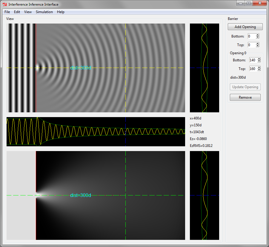
Figure 2: The single narrow slit simulation.

See Figure 2. This simulation provides a baseline for comparison. It shows that a single narrow opening is not responsible for the interference patterns seen in the following simulations.

The course’s lectures included a mathematical description of point sources in 3D, so this simulation introduced students to the asymmetric sources used in the laboratory. To acquaint students with the simulation’s controls, I had them roughly measure how fast the amplitude decreased with distance from the opening; because this is a 2D simulation, the amplitude falls off less quickly than in 3D.

III.2 Narrow Double Slits

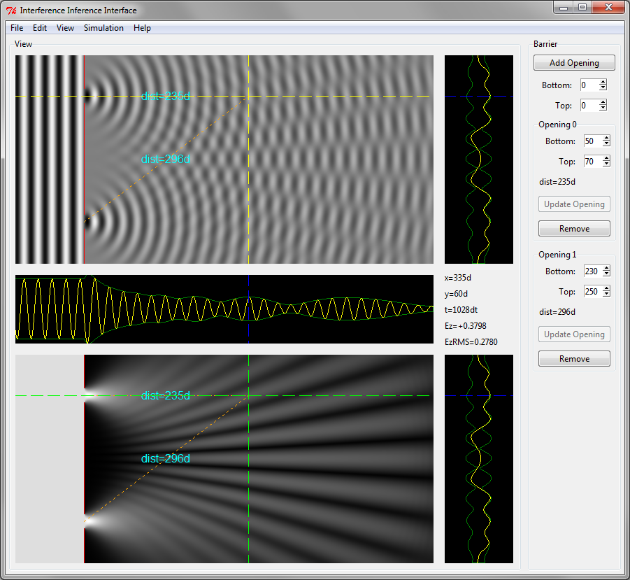
Figure 3: The double narrow slit simulation with the dashed lines intersecting at an $E_{zRMS}$ maximum.

See Figure 3. This is the key simulation; it lets students discover the conditions for constructive and destructive interference. Students were asked to find four maxima and four minima of $E_{zRMS}$—in either $\hat{x}$ or $\hat{y}$ and in the right half of the domain, calculate $\frac{\left|d_{0}-d_{1}\right|}{\lambda}$ for each—where $d_{0}$ and $d_{1}$ are the distances from the extrema to the openings, and then find the pattern in those numbers.

In principle, the students already knew the conditions, but they seemed new to many. Furthermore, most students seemed to be comprehending the conditions for the first time. Pen and paper work followed to reinforce their understanding. This included drawing a couple waves that resulted in those conditions (using a simplified version ofdrawing1 ; drawing2 ) and mathematically verifying that the conditions lead to waves in or out of phase.

III.3 Narrow Triple Slits

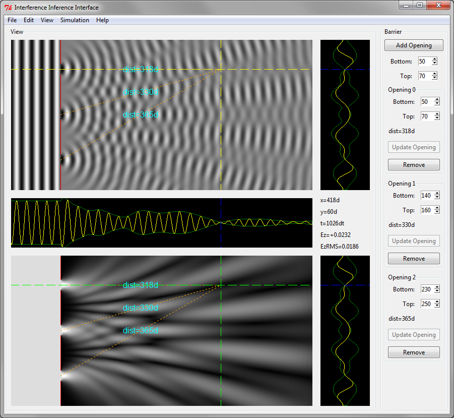
Figure 4: The triple narrow slit simulation with the dashed lines intersecting at an $E_{zRMS}$ minimum. It is located $15.9\lambda$, $16.5\lambda$, and $18.25\lambda$ from the three openings.

See Figure 4. The additional slit makes students closely consider the logic behind the extrema conditions.

Here, the students were asked to find points that were simultaneously extrema in both $\hat{x}$ and $\hat{y}$. This is straightforward with the simulation, but—since this requires fine control in both $\hat{x}$ and $\hat{y}$—this would be difficult using the standard experimental setup.

The condition for constructive interference still holds. To get a maximum, all pairs should be maximized.

However, the minimization condition is more complicated.Ovchinnikov200333 The two slit condition caused the two waves to roughly cancel. That would leave the third wave undiminished. Additionally, it is mathematically impossible for all differences in the distances to be a half integer number of wavelengths.

This is an instructive example that is missing from laboratories that do not use simulations for quantitative measurements.

III.4 Wide Single Slit

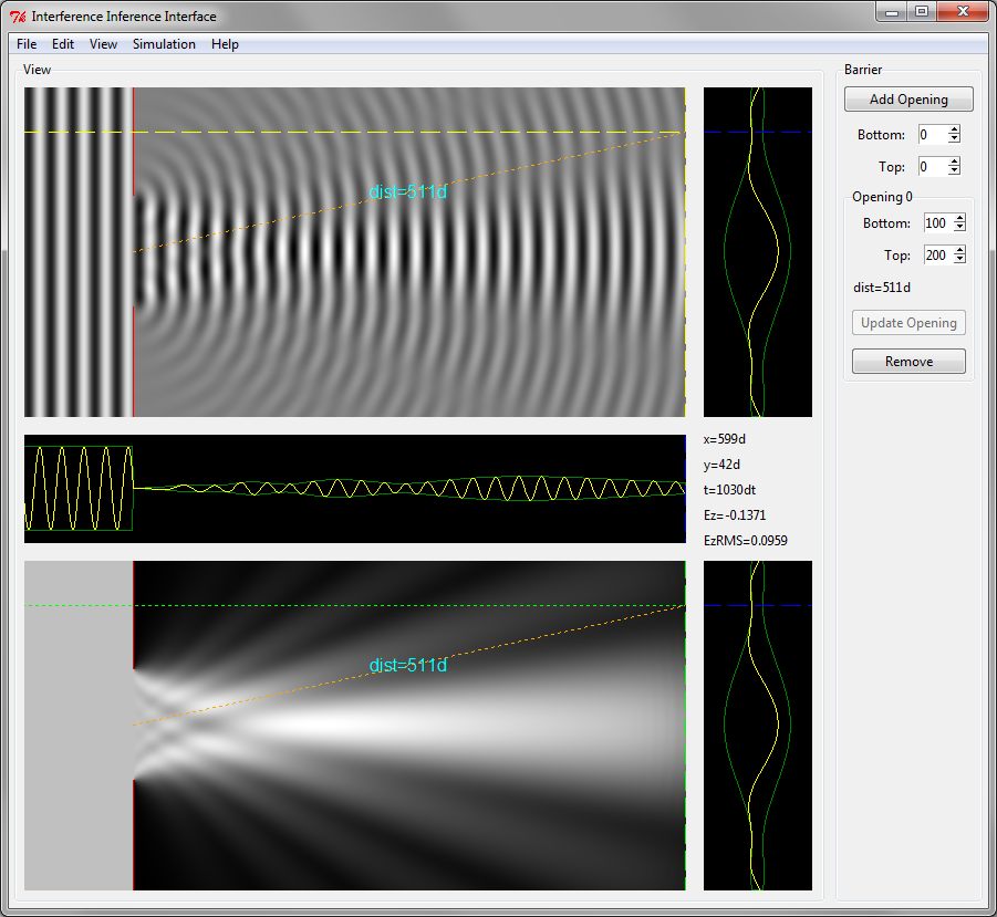
Figure 5: The wide single slit simulation with the dashed lines intersecting at the first minimum. It occurs at $\theta=\arctan\left(\frac{150-42}{599-100}\right)=0.213$, whereas the far field limit has $\theta=\frac{20}{100}=0.2$.

See Figure 5. The right side of the domain gets close to the far field limit. While the domain is too small to truly display far field effects—a limitation common to many ripple tanks, the simulation successfully shows diffraction effects arising from waves. The simulation could be used to investigate near field effects—something difficult with normal instructional laboratory equipment.

IV Results

Table 1: Scores for point C. The first three columns of results are from Wosilait et al. and are rounded to the nearest 5%.wosilait:S5

	Old UWash	UWash Grad	New UWash	My 15
Right Method	10%	55%	70%	73%
and Right Answer	5%	25%	45%	60%

Only $15$ students used the finial version of the laboratory, so the only conclusion I can draw with confidence is that students enjoyed it; I collected anonymous feedback, and it was overwhelmingly positive. Still, for a rough gauge of the method’s effectiveness, I quizzed the students with questions from the University of Washington study. Scores for point C are in Table 1.

They did well on all parts of the quiz, relative to others. $60\%$ of the students answered correctly for point C. $80\%$ correctly identified the behavior at both points A and B—students in the old University of Washington system scored $35\%$.wosilait:S5 The quiz included another question from the University of Washington study. See Figure 6. What would be observed at the far away point—first with just the left two slits and then with all three slits? $80\%$ got both parts right.

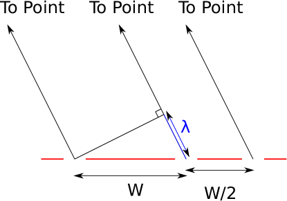
Figure 6: Figure for the second quiz question.

V Conclusion

Interference and diffraction are tricky subjects to teach, but this approach shows promise in making them more accessible to students. The simulation allows them to easily control, visualize, and quantitatively measure interference and diffraction effects. That makes the software a powerful tool.

The progression of simulations described here appears effective. First, a single narrow slit familiarized students with the simulation and showed more was needed for interference. Then, a double slit simulation showed Young’s experiment in a new light, with visible waves and easy measurements. Next, a triple slit experiment made students reconsider the constructive and destructive interference conditions; one held but the other fell. Finally, a diffraction simulation showed that similar effects could arise from one wide slit.

While the sample size here was small, the results are encouraging. I hope eventually to try this approach with more students in more classes.

It would be difficult to experimentally mimic some of the simulations with instructional laboratory equipment. The simulation could also easily demonstrate more advanced topics with minimal modification. The permittivity, permeability, and conductivity are definable at every point in the simulation domain. Changing those parameters would allow the simulation to demonstrate waveguides, reflection due to changes in dielectric constants, etc. Simulations of a modified two slit experiment—where the upper and lower halves of the domain have different indices of refraction—could illustrate more conceptual topics, like the difference between physical and optical path length.opticalPath

- [1] Karen Wosilait, Paula R. L. Heron, Peter S. Shaffer, and Lillian C. McDermott. Addressing student difficulties in applying a wave model to the interference and diffraction of light. Am. J. Phys., 67(S1):S5–S15, 1999.
- [2] Bradley S. Ambrose, Peter S. Shaffer, Richard N. Steinberg, and Lillian C. McDermott. An investigation of student understanding of single-slit diffraction and double-slit interference. Am. J. Phys., 67(2):146–155, 1999.
- [3] PASCO scientific. Ripple generator and light source manual (wa-9896).
- [4] Nuffield Foundation. Measuring Waves in a ripple tank. Available online http://www.nuffieldfoundation.org/practical-physics/measuring-waves-ripple tank.
- [5] Sergey Vtorov. Interference. Simulation available at http://vsg.quasihome.com/interfer.htm.
- [6] Marvin De Jong. Using computer-generated animations as an aid in teaching wave motion and sound. The Physics Teacher, 41(9):524–529, 2003.
- [7] Melissa Dancy, Wolfgang Christian, and Mario Belloni. Teaching with physlets®: Examples from optics. The Physics Teacher, 40(8):494–499, 2002.
- [8] Taha Mzoughi, S. Davis Herring, John T. Foley, Matthew J. Morris, and Peter J. Gilbert. Webtop: A 3d interactive system for teaching and learning optics. Computers & Education, 49(1):110 – 129, 2007.
- [9] J. Frances, M. Perez-Molina, S. Bleda, E. Fernandez, C. Neipp, and A. Belendez. Educational software for interference and optical diffraction analysis in fresnel and fraunhofer regions based on matlab guis and the fdtd method. IEEE Trans. Edu., 55(1):118 –125, 2012.
- [10] Christopher A. Werley, Keith A. Nelson, and C. Ryan Tait. Direct visualization of terahertz electromagnetic waves in classic experimental geometries. Am. J. Phys., 80(1):72–81, 2012.
- [11] Kane Yee. Numerical solution of initial boundary value problems involving maxwell’s equations in isotropic media. IEEE Trans. Antennas Propag., 14(3):302 –307, 1966.
- [12] A. Taflove and S.C. Hagness. Computational Electrodynamics: The Finite-Difference Time-Domain Method. Artech House, 2005.
- [13] M. Sipos and B. G. Thompson. Electrodynamics on a grid: The finite-difference time-domain method applied to optics and cloaking. Am. J. Phys., 76(4-5):464–469, 2008.
- [14] Jean-Pierre Berenger. A perfectly matched layer for the absorption of electromagnetic waves. J Comput. Phys., 114(2):185 – 200, 1994.
- [15] David Chandler. Simulate interference…while supplies last. The Physics Teacher, 39(6):362–363, 2001.
- [16] David Kagan. Simulate interference…with supplies that last. The Physics Teacher, 47(4):246–246, 2009.
- [17] Fresnel interference pattern of a triple-slit interferometer. Optics Commun., 216(1-3):33–40, 2003.
- [18] Ronald Newburgh. Optical path, phase, and interference. The Physics Teacher, 43(8):496–498, 2005.