Meson–Photon Transition Form Factors

Abstract

We present the results of our recent analysis of the meson–photon transition form factors $F_{P\gamma}(Q^{2})$ for the pseudoscalar mesons $P=\pi^{0},\eta,\eta^{\prime},\eta_{c}$, using the local-duality version of QCD sum rules.

1 Introduction

The processes $\gamma^{*}\,\gamma^{*}\to P$ with $P=\pi^{0},\eta,\eta^{\prime},\eta_{c}$ are of great interest for our understanding of QCD and of the meson structure. In recent years, extensive experimental information on these processes has become available cello-cleo ; babar1 ; babar ; babar2010 ; belle .

The corresponding amplitude contains only one form factor, $F_{P\gamma\gamma}(q_{1}^{2},q_{2}^{2})$:

$$\langle\gamma^{*}(q_{1})\gamma^{*}(q_{2})|P(p)\rangle={\rm i}\epsilon_{\varepsilon_{1}\varepsilon_{2}q_{1}q_{2}}F_{P\gamma\gamma}(q_{1}^{2},q_{2}^{2}).$$ (1)

A QCD factorization theorem predicts this form factor at asymptotically large spacelike momentum transfers $q_{1}^{2}\equiv-Q_{1}^{2}\leq 0$, $q_{2}^{2}\equiv-Q_{2}^{2}\leq 0$ brodsky :

$$F_{P\gamma\gamma}(Q_{1}^{2},Q_{2}^{2})\to 2e_{c}^{2}\int\limits_{0}^{1}\frac{{\rm d}\xi\phi^{\rm ass}_{P}(\xi)}{Q_{1}^{2}\xi+Q_{2}^{2}(1-\xi)},\qquad\phi^{\rm ass}_{P}(\xi)=6f_{P}\xi(1-\xi).$$ (2)

Hereafter, we use the notation $Q^{2}\equiv Q_{2}^{2}$ and $0\leq\beta\equiv Q_{1}^{2}/Q_{2}^{2}\leq 1$ (that is, $Q_{2}^{2}$ is the larger virtuality). For the experimentally relevant kinematics $Q_{1}^{2}\approx 0$ and $Q_{2}^{2}\equiv Q^{2}$, for instance, the pion–photon transition form factor takes the form

$$Q^{2}F_{\pi\gamma}(Q^{2})\to\sqrt{2}f_{\pi},\qquad f_{\pi}=0.130\;\mbox{GeV}.$$ (3)

Similar relations arise for $\eta$ and $\eta^{\prime}$ after taking into account the effects of meson mixing.

2 Dispersive sum rules for the $\gamma^{*}\,\gamma^{*}\to P$ form factor

The starting point for a QCD sum-rule analysis of the $\gamma^{*}\,\gamma^{*}\to P$ transition form factor is the amplitude

$$\langle 0|j_{\mu}^{5}|\gamma^{*}(q_{2})\gamma^{*}(q_{1})\rangle=e^{2}T_{\mu\alpha\beta}(p|q_{1},q_{2})\,\varepsilon^{\alpha}_{1}\varepsilon^{\beta}_{2},\qquad p=q_{1}+q_{2},$$ (4)

where $\varepsilon_{1,2}$ are the relevant photon polarization vectors. This amplitude is considered for $-q_{1}^{2}\equiv Q_{1}^{2}\geq 0$ and $-q_{2}^{2}\equiv Q_{2}^{2}\geq 0$. Its general decomposition contains four independent Lorentz structures (see e.g. Refs. blm2011 ; lm2011 ) but for our purpose only one structure is needed:

$$T_{\mu\alpha\beta}(p|q_{1},q_{2})=p_{\mu}\epsilon_{\alpha\beta q_{1}q_{2}}{\rm i}F(p^{2},Q_{1}^{2},Q_{2}^{2})+\cdots.$$ (5)

The corresponding invariant amplitude $F(p^{2},Q_{1}^{2},Q_{2}^{2})$ satisfies the spectral representation in $p^{2}$ at fixed $Q_{1}^{2}$ and $Q_{2}^{2}$

$$F(p^{2},Q_{1}^{2},Q_{2}^{2})=\frac{1}{\pi}\int\limits_{s_{\rm th}}^{\infty}\frac{{\rm d}s}{s-p^{2}}\,\Delta(s,Q_{1}^{2},Q_{2}^{2}),$$ (6)

where $\Delta(s,Q_{1}^{2},Q_{2}^{2})$ is the physical spectral density and $s_{\rm th}$ denotes the physical threshold.

Perturbation theory yields the spectral density as a series expansion in powers of $\alpha_{s}$:

$$\Delta_{\rm pQCD}(s,Q_{1}^{2},Q_{2}^{2}|m)=\Delta^{(0)}_{\rm pQCD}(s,Q_{1}^{2},Q_{2}^{2}|m)+\frac{\alpha_{s}}{\pi}\Delta^{(1)}_{\rm pQCD}(s,Q_{1}^{2},Q_{2}^{2}|m)+\cdots,$$ (7)

where $m$ is the mass of the quark propagating in the loop. The lowest-order contribution, $\Delta^{(0)}_{\rm pQCD}(s,Q_{1}^{2},Q_{2}^{2}|m)$, corresponding to a one-loop triangle diagram with one axial current and two vector currents at the vertices, is well-known 1loop . The two-loop $O(\alpha_{s})$ correction to the spectral density was found to vanish 2loop . Higher-order corrections are unknown.

The physical spectral density differs dramatically from $\Delta_{\rm pQCD}(s,Q_{1}^{2},Q_{2}^{2})$ in the low-$s$ region; it contains the meson pole and the hadronic continuum. For instance, in the $I=1$ channel, one has

$$\Delta(s,Q_{1}^{2},Q_{2}^{2})=\pi\delta(s-m_{\pi}^{2})\,\sqrt{2}f_{\pi}\,F_{\pi\gamma\gamma}(Q^{2}_{1},Q_{2}^{2})+\theta(s-s_{\rm th})\,\Delta^{I=1}_{\rm cont}(s,Q^{2}_{1},Q_{2}^{2}).$$ (8)

The method of QCD sum rules allows one to relate the properties of the ground states to the spectral densities of QCD correlators. The following steps are conventional within the QCD sum-rule method lms1 ; lms2 : equate the QCD and the physical representations for $F(p^{2},Q_{1}^{2},Q_{2}^{2})$; then perform the Borel transform $p^{2}\to\tau,$ which suppresses the hadronic continuum; in order to kill then potentially dangerous nonperturbative power corrections which may rise with $Q^{2}$, take the local-duality (LD) limit $\tau=0$ ld ; finally, implement quark–hadron duality in a standard way as low-energy cut on the spectral representation, in order to arrive at the following expression for the ground-state transition form factor:

$$\pi f_{P}F_{P\gamma\gamma}(Q_{1}^{2},Q_{2}^{2})=\int\limits_{4m^{2}}^{s_{\rm eff}(Q_{1}^{2},Q_{2}^{2})}{\rm d}s\,\Delta_{\rm pQCD}(s,Q_{1}^{2},Q_{2}^{2}|m).$$ (9)

All details of the nonperturbative-QCD dynamics are contained in the effective threshold $s_{\rm eff}(Q_{1}^{2},Q_{2}^{2})$. The formulation of reliable criteria for fixing effective thresholds proves to be highly nontrivial lms1 .

At large $Q_{2}^{2}\equiv Q^{2}\to\infty$ and fixed ratio $\beta\equiv Q_{1}^{2}/Q_{2}^{2}$, the effective threshold $s_{\rm eff}(Q_{1}^{2},Q_{2}^{2})$ may be determined by suitable matching to the asymptotic pQCD factorization formula. From this, one finds that, in the general case $m\neq 0$, $s_{\rm eff}(Q^{2}\to\infty,\beta)$ depends on $\beta$. The only exception to this is the case of massless fermions, $m=0$: in this case the asymptotic factorization formula is reproduced for any $\beta$ if one sets $s_{\rm eff}(Q^{2}\to\infty,\beta)=4\pi^{2}f_{\pi}^{2}.$ The LD model for the transition form factor emerges when one assumes that, at finite values of $Q^{2}$, $s_{\rm eff}(Q^{2},\beta)$ may be sufficiently well approximated by its value for $Q^{2}\to\infty$, that is,

$$s_{\rm eff}(Q^{2},\beta)=s_{\rm eff}(Q^{2}\to\infty,\beta).$$ (10)

Introducing the abbreviation $F_{P\gamma}(Q^{2})\equiv F_{P\gamma\gamma}(0,Q^{2})$ for the pseudoscalar-meson–photon transition form factor, its LD expression for $Q_{1}^{2}=0$ and $m=0$ reads, in the single-flavour case,

$$F_{P\gamma}(Q^{2})=\frac{1}{2\pi^{2}f_{P}}\frac{s_{\rm eff}(Q^{2})}{s_{\rm eff}(Q^{2})+Q^{2}}.$$ (11)

Independently of the behaviour of $s_{\rm eff}(Q^{2})$ at $Q^{2}\to 0$, $F_{P\gamma}(Q^{2}=0)$ is related to the axial anomaly blm2011 .

3 The transition $\gamma\,\gamma^{*}\to P$ in quantum mechanics

The accuracy of the LD model for the effective threshold may be estimated in quantum mechanics. There, the form factor may be found exactly by some numerical solution Lucha98 of the Schrödinger equation. From this, the exact effective threshold may be calculated: for any given experimental or theoretical form factor, the corresponding exact effective threshold is defined as the quantity that reproduces this form factor by a LD sum rule (9).

The result from a quantum-mechanical model with a harmonic-oscillator potential blm2011 is shown in Fig. 1. For “light” quarks, the LD threshold gives a very good approximation to the exact threshold for $Q>1$–$1.5\;\mbox{GeV}$. For “charm” quarks, the local-duality model works for $Q>2$–$3\;\mbox{GeV}$. The accuracy of the LD approximation further increases with $Q$ in this region.

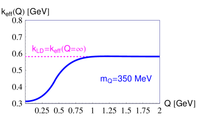
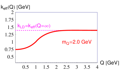
Figure 1: The exact effective threshold in quantum mechanics, $k_{\rm eff}(Q)$, for two different values of the nonrelativistic constituent quark mass $m_{Q}$.

4 $\gamma^{*}\,\gamma^{*}\to\eta_{c}$ form factor

In the case of massive quarks, we may exploit not only the correlation function $\langle AVV\rangle$ as in Eq. (4) but also the correlation function $\langle PVV\rangle$ lm2011 . For each of these objects, an LD model may be constructed. By matching to the pQCD factorization formula, we derive $s_{\rm eff}(Q^{2}\to\infty,\beta)$ for $\langle AVV\rangle$ and for $\langle PVV\rangle$. The results of the corresponding calculation for $\eta_{c}$ are depicted in Fig. 2. Obviously, the exact effective thresholds corresponding to $\langle AVV\rangle$ and $\langle PVV\rangle$, $s_{\rm eff}^{AVV}(Q^{2}\to\infty,\beta)$ and $s_{\rm eff}^{PVV}(Q^{2}\to\infty,\beta),$ differ from each other; they also differ from the effective thresholds of the relevant two-point correlation functions.

Assuming that $s_{\rm eff}(Q^{2},\beta)=s_{\rm eff}(Q^{2}\to\infty,\beta)$, we obtain the results shown in Fig. 2. For the above reasons, at very small $Q^{2}$ the applicability of our LD model is not guaranteed. Nevertheless, applying our LD model down to $Q^{2}=0$ predicts $F_{\eta_{c}\gamma}(0)=0.067\;\mbox{GeV}^{-1}$ from the analysis of $\langle AVV\rangle$ and $F_{\eta_{c}\gamma}(0)=0.086\;\mbox{GeV}^{-1}$ from the analysis of $\langle PVV\rangle$; this has to be compared with the experimental number $F_{\eta_{c}\gamma}(Q^{2}=0)=0.08\pm 0.01\;\mbox{GeV}^{-1}.$ Seemingly, the LD model based on the correlator $\langle PVV\rangle$ gives reliable predictions for a broad range of momentum transfers $Q^{2}$ starting even at very low values of $Q^{2}$ (cf. kroll ).

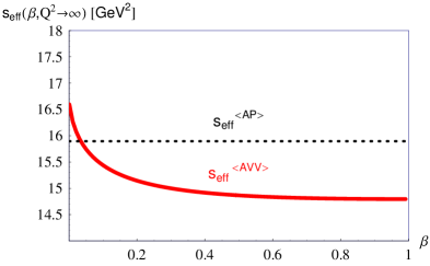
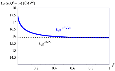
(a)	(b)
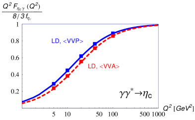
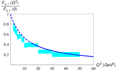
(c)	(d)

Figure 2: Form factor for the transition $\gamma\,\gamma^{*}\to\eta_{c}$: exact effective thresholds $s_{\rm eff}^{AVV}(Q^{2}\to\infty,\beta)$ (a) and $s_{\rm eff}^{PVV}(Q^{2}\to\infty,\beta)$ (b); form factors obtained for finite $Q^{2}$ from the LD sum rules for the correlators $\langle AVV\rangle$ and $\langle PVV\rangle$ (c); LD model for the correlator $\langle PVV\rangle$ confronted with experimental data by BaBar babar2010 (d).

5 $\gamma\,\gamma^{*}\to(\eta,\eta^{\prime})$ form factors

Here, the mixing of strange and nonstrange components mixing must be taken into account:

$$F_{\eta\gamma}=F_{n\gamma}\cos\phi-F_{s\gamma}\sin\phi,\qquad F_{\eta^{\prime}\gamma}=F_{n\gamma}\sin\phi+F_{s\gamma}\cos\phi,\qquad\phi\approx 38^{0},$$ (12)

with $n\to(\bar{u}u+\bar{d}d)/\sqrt{2}$ and $s\to\bar{s}s$. The LD expressions for these two form factors read

$$F_{n\gamma}(Q^{2})=\frac{1}{f_{n}}\int\limits_{0}^{s_{\rm eff}^{(n)}(Q^{2})}{\rm d}s\,\Delta_{n}(s,Q^{2}),\qquad F_{s\gamma}(Q^{2})=\frac{1}{f_{s}}\int\limits_{0}^{s_{\rm eff}^{(s)}(Q^{2})}{\rm d}s\,\Delta_{s}(s,Q^{2}).$$ (13)

Accordingly, two separate effective thresholds emerge: $s_{\rm eff}^{(n)}=4\pi^{2}f_{n}^{2}$, $s_{\rm eff}^{(s)}=4\pi^{2}f_{s}^{2}$, with $f_{n}\approx 1.07f_{\pi}$, $f_{s}\approx 1.36f_{\pi}$. The outcomes from the LD model blm2011 ; lm2011 and the experimental data cello-cleo ; babar1 are in reasonable agreement with each other (Fig. 3).

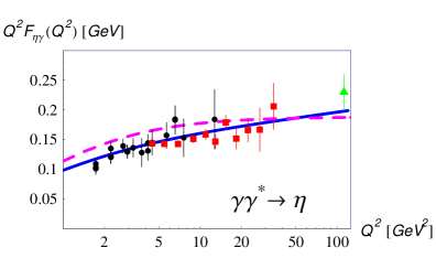
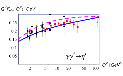
Figure 3: $\gamma\,\gamma^{*}\to(\eta,\eta^{\prime})$ transition form factors $F_{(\eta,\eta^{\prime})\gamma}(Q^{2})$: LD predictions blm2011 ; lm2011 (dashed lines) and recent fits ms2012 (solid lines) to the experimental data cello-cleo ; babar1 .

6 $\gamma\,\gamma^{*}\to\pi^{0}$ form factor

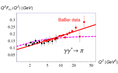
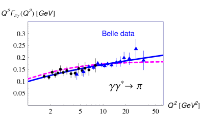
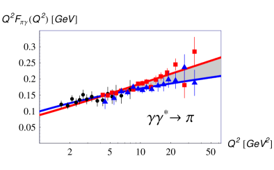
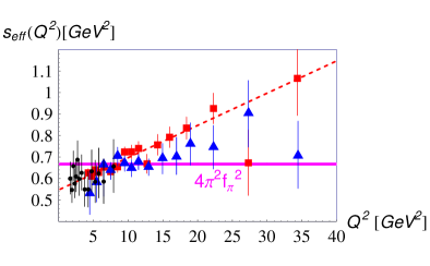
Figure 4: $\gamma\,\gamma^{*}\to\pi^{0}$ transition form factor $F_{\pi\gamma}(Q^{2})$: LD prediction (magenta lines) and a fit ms2012 (solid lines) to the data cello-cleo ; babar ; belle . The equivalent effective threshold $s_{\rm eff}(Q^{2})$ for each data point is found via (11).

First of all, we emphasize that the large-$Q^{2}$ behaviour of the $\eta$, $\eta^{\prime}$, and $\pi^{0}$ form factors is determined by the spectral densities of perturbative QCD diagrams and should therefore be the same for all light pseudoscalars ms2012 . In order to demonstrate this, we observe that the sum rule for $\langle AVV\rangle$ in the LD limit $\tau=0$ is equivalent to the anomaly sum rule teryaev2

$$F_{\pi\gamma}(Q^{2})=\frac{1}{2\sqrt{2}\,\pi^{2}f_{\pi}}\left[1-2\pi\int\limits_{s_{\rm th}}^{\infty}{\rm d}s\,\Delta^{I=1}_{\rm cont}(s,Q^{2})\right].$$ (14)

Similar relations arise for the $I=0$ and the $\bar{s}s$ channels. As shown in Ref. ms2012 , the form factors $F_{\pi\gamma}(Q^{2})$, $F_{\eta\gamma}(Q^{2})$, and $F_{\eta^{\prime}\gamma}(Q^{2})$ at large $Q^{2}$ are determined by the behaviour of the appropriate $\Delta_{\rm cont}(s,Q^{2})$ at large $s$. By quark–hadron duality, the latter are equal to the corresponding $\Delta_{\rm pQCD}(s,Q^{2})$; these are purely perturbative quantities and therefore equal to each other for the different channels.

However, the BaBar data for the $\pi$ transition form factor exhibit a clear disagreement with both the $\eta$, $\eta^{\prime}$ form factors and the LD model at $Q^{2}$ as large as $40\;\mbox{GeV}^{2}$. Moreover, opposite to findings in quantum mechanics, the violations of LD rise with $Q^{2}$ even in the region $Q^{2}\approx 40\;\mbox{GeV}^{2}$! We thus conclude that the BaBar results are hard to understand in QCD (see also findings ). Noteworthy, recent Belle measurements of the $\pi\gamma$ form factor—although being statistically consistent with the BaBar findings (see agaev ; pere )—are fully compatible with the $\eta$ and $\eta^{\prime}$ data as well as with the onset of the LD regime already in the region $Q^{2}\geq 5$–$10\;\mbox{GeV}^{2}$, in full agreement with our quantum-mechanical experience.

7 Conclusions

We studied the $\pi^{0}$, $\eta$, $\eta^{\prime}$, and $\eta_{c}$ transition form factors by QCD sum rules in LD limit; the key parameter—the effective continuum threshold—was determined by matching the LD form factors to QCD factorization formulas. Our main conclusions are the following:

$\bullet$ For all $P\to\gamma\,\gamma^{*}$ form factors studied, the LD model should work well in a region of $Q^{2}$ larger than a few GeV²: the LD model works reasonably well for the $\eta\to\gamma\,\gamma^{*}$, $\eta^{\prime}\to\gamma\,\gamma^{*}$, and $\eta_{c}\to\gamma\,\gamma^{*}$ form factors. For $\pi^{0}\to\gamma\,\gamma^{*}$, the BaBar data indicate an extreme violation of local duality, prompting a linearly rising (instead of a constant) effective threshold. In contrast to this, the Belle data exhibit an agreement with the predictions of the LD model.

$\bullet$ Nevertheless, a better fit to the full set of the meson–photon form-factor data seems to prefer a small logarithmic rise of $Q^{2}F_{P\gamma}(Q^{2})$ ms2012 . If established experimentally, this rise would require the presence of a $1/s$ duality-violating term in the ratio of the hadron and the QCD spectral densities.

$\bullet$ A high accuracy of the LD model has implications for the pion’s elastic form factor: we can show that the accuracy of the LD model for the elastic form factor increases with $Q^{2}$ in the region $Q^{2}\approx 4$–$8\;\mbox{GeV}^{2}$ blm2011 . The accurate data on the pion form factor suggest that the LD limit for the effective threshold, $s_{\rm eff}(Q^{2}\to\infty)=4\pi^{2}f_{\pi}^{2}$, may be reached already at $Q^{2}=5$–$6\;\mbox{GeV}^{2}$. This property should be testable with the JLab upgrade CLAS12.

References

- (1) H. J. Behrend et al., Z. Phys. C 49, 401 (1991); J. Gronberg et al., Phys. Rev. D 57, 33 (1998).
- (2) B. Aubert et al., Phys. Rev. D 80, 052002 (2009).
- (3) J. P. Lees et al., Phys. Rev. D 81, 052010 (2010).
- (4) P. del Amo Sanchez et al., Phys. Rev. D 84, 052001 (2011).
- (5) S. Uehara et al., arXiv:1205.3249.
- (6) G. P. Lepage and S. J. Brodsky, Phys. Rev. D 22, 2157 (1980).
- (7) V. Braguta, W. Lucha, and D. Melikhov, Phys. Lett. B 661, 354 (2008); I. Balakireva, W. Lucha, and D. Melikhov, J. Phys. G 39, 055007 (2012) [arXiv:1103.3781]; Phys. Rev. D 85, 036006 (2012); Phys. Atom. Nucl. 75 (2012) (in press) [arXiv:1203.2599].
- (8) W. Lucha and D. Melikhov, J. Phys. G 39, 045003 (2012) [arXiv:1110.2080]; Phys. Rev. D 86, 016001 (2012) [arXiv:1205.4587].
- (9) J. Hořejší and O. V. Teryaev, Z. Phys. C 65, 691 (1995); D. Melikhov and B. Stech, Phys. Rev. Lett. 88, 151601 (2002); D. Melikhov, Eur. Phys. J. direct C4, 2 (2002) [arXiv:hep-ph/0110087].
- (10) F. Jegerlehner and O. V. Tarasov, Phys. Lett. B 639, 299 (2006); R. S. Pasechnik and O. V. Teryaev, Phys. Rev. D 73, 034017 (2006).
- (11) W. Lucha, D. Melikhov, and S. Simula, Phys. Rev. D 76, 036002 (2007); Phys. Lett. B 657, 148 (2007); Phys. Atom. Nucl. 71, 1461 (2008); Phys. Lett. B 671, 445 (2009); D. Melikhov, Phys. Lett. B 671, 450 (2009).
- (12) W. Lucha, D. Melikhov, and S. Simula, Phys. Rev. D 79, 096011 (2009); J. Phys. G 37, 035003 (2010) [arXiv:0905.0963]; Phys. Lett. B 687, 48 (2010); Phys. Atom. Nucl. 73, 1770 (2010); J. Phys. G 38, 105002 (2011) [arXiv:1008.2698]; Phys. Lett. B 701, 82 (2011); W. Lucha, D. Melikhov, H. Sazdjian, and S. Simula, Phys. Rev. D 80, 114028 (2009).
- (13) V. A. Nesterenko and A. V. Radyushkin, Phys. Lett. B 115, 410 (1982).
- (14) W. Lucha and F. F. Schöberl, Int. J. Mod. Phys. C 10, 607 (1999).
- (15) P. Kroll, Eur. Phys. J. C 71, 1623 (2011).
- (16) V. V. Anisovich, D. I. Melikhov, and V. A. Nikonov, Phys. Rev. D 55, 2918 (1997); V. V. Anisovich, D. V. Bugg, D. I. Melikhov, and V. A. Nikonov, Phys. Lett. B 404, 166 (1997); T. Feldmann, P. Kroll, and B. Stech, Phys. Rev. D 58, 114006 (1998); Phys. Lett. B 449, 339 (1999).
- (17) D. Melikhov and B. Stech, Phys. Rev. D 85, 051901 (2012); arXiv:1206.5764.
- (18) Y. N. Klopot, A. G. Oganesian, and O. V. Teryaev, Phys. Lett. B 695, 130 (2011); Phys. Rev. D 84, 051901 (2011).
- (19) H. L. L. Roberts et al., Phys. Rev. C 82, 065202 (2010); S. J. Brodsky, F.-G. Cao, and G. F. de Téramond, Phys. Rev. D 84, 033001 (2011); 84, 075012 (2011); A. P. Bakulev, S. V. Mikhailov, A. V. Pimikov, and N. G. Stefanis, Phys. Rev. D 84, 034014 (2011); arXiv:1205.3770.
- (20) S. S. Agaev, V. M. Braun, N. Offen, and F. A. Porkert, Phys. Rev. D 83, 054020 (2011); arXiv: 1206.3968.
- (21) P. Masjuan, arXiv:1206.2549.