Three dimensional particle-in-cell simulation of particle acceleration by circularly polarised inertial Alfven waves in a transversely inhomogeneous plasma

Abstract

The process of particle acceleration by left-hand, circularly polarised inertial Alfven waves (IAW) in a transversely inhomogeneous plasma is studied using 3D particle-in-cell simulation. A cylindrical tube with, transverse to the background magnetic field, inhomogeneity scale of the order of ion inertial length is considered on which IAWs with frequency $0.3\omega_{ci}$ are launched that are allowed to develop three wavelength. As a result time-varying parallel electric fields are generated in the density gradient regions which accelerate electrons in the parallel to magnetic field direction. Driven perpendicular electric field of IAWs also heats ions in the transverse direction. Such numerical setup is relevant for solar flaring loops and earth auroral zone. This first, 3D, fully-kinetic simulation demonstrates electron acceleration efficiency in the density inhomogeneity regions, along the magnetic field, of the order of 45% and ion heating, in the transverse to the magnetic field direction, of 75%. The latter is a factor of two times higher than the previous 2.5D analogous study and is in accordance with solar flare particle acceleration observations. We find that the generated parallel electric field is localised in the density inhomogeneity region and rotates in the same direction and with the same angular frequency as the initially launched IAW. Our numerical simulations seem also to suggest that the ”knee” often found in the solar flare electron spectra can alternatively be interpreted as the Landau damping (Cerenkov resonance effect) of IAWs due to the wave-particle interactions.

I Introduction

Super-thermal particles play an important role in many space plasma situations. The relevant two examples are: (i) Earths Auroral zone (AZ) that is known to host strong field-aligned currents, parallel electric field and accelerated particles. Observations essentially show two modes of particle acceleration present in AZ: a) Precipitating auroral electrons narrowly peaked at specific energy, suggestive of a static potential drop in the AZ (e.g. Ref.Mozer et al. (1980)); b) More recent observations by FAST spacecraft (e.g. Ref.Chaston et al. (2007)) indicate existence of electrons with broad energy and narrow in pitch angle distribution that is consistent with the inertial Alfven wave (IAW) acceleration. (ii) In solar corona, a significant fraction of the energy released during solar flares is converted into the energy of accelerated particles Emslie et al. (2004). The parallel electric field that can accelerate electrons is produced when low frequency ($\omega<\omega_{ci}$, where $\omega_{ci}=eB/m_{i}$ is the ion cyclotron frequency) dispersive Alfven wave (DAW) has a wavelength perpendicular to the background magnetic field comparable to any of the kinetic spatial scales such as: ion gyroradius at electron temperature, $\rho_{s}=\sqrt{k_{B}T_{e}/m_{i}}/\omega_{ci}$, ion thermal gyroradius, $\rho_{i}=\sqrt{k_{B}T_{i}/m_{i}}/\omega_{ci}$, Hasegawa (1976) or to electron inertial length $\lambda_{e}=c/\omega_{pe}$ Goertz and Boswell (1979). Dispersive Alfven waves are divided into Inertial Alfven Waves or Kinetic Alfven Waves (KAW) depending on the relation between the plasma $\beta$ and electron/ion mass ratio $m_{e}/m_{i}$ Stasiewicz et al. (2000). When $\beta\ll m_{e}/m_{i}$ (i.e. when Alfven speed is much greater than electron and ion thermal speeds, $V_{A}\gg v_{th,i},v_{th,e}$) dominant mechanism for sustaining $E_{\parallel}$ is the parallel electron inertia and such waves are called Inertial Alfven Waves. When $\beta\gg m_{e}/m_{i}$, (i.e. when $V_{A}\ll v_{th,i},v_{th,e}$) then thermal effects become important and the dominant mechanism for supporting $E_{\parallel}$ is the parallel electron pressure gradient. Such waves are called Kinetic Alfven Waves.

The context of this study is related to the theoretical plasma physics processes operating in the particle acceleration in solar flares. Ref.Brown et al. (2009)’s Introduction gives a good overview of both theoretical and observational unresolved issues. If the solar flare particle acceleration happens in the corona, in order to explain the observed X-ray flux as the electrons smash into the dense layers of the Sun, implausibly large acceleration region volumes and/or densities are required. Different ideas have been put forward: (i) Substantial re-acceleration in the chromosphere of electrons accelerated in and injected from the corona can greatly reduce the density and number of fast electrons needed to produce a X-ray flux Brown et al. (2009); However, this still seems problematic because recent analysis of the evolution of a radio spectrum from a dense flare Bastian et al. (2007) (Bastian et al. 2007) shows that a significant fraction of the energy in the energetic electrons can be deposited into the coronal loop, as opposed to into the chromosphere. The estimates show that the energy deposited in the corona can approach about 30% flare energy. (ii) The electric circuit formed by precipitating and returning electrons Zharkova et al. (2011a, b). The effect was found from the Ampere law which handles the circuit of injected and returning electrons when simulated with Particle-In-Cell and Fokker-Planck simulations. (iii) When wave-particle interactions in non-uniform plasma are taken into account, the evolution of the Langmuir wave spectrum towards smaller wave-numbers, leads to an effective acceleration of electrons. Thus, the time-integrated spectrum of non-thermal electrons shows an increase in super-thermal electrons, because of their acceleration by the Langmuir waves Kontar et al. (2012). (iv) Solar flare triggered DAWs, as opposed to the electron beams, propagating towards the solar coronal loop foot-points, and accelerating electrons along the propagation paths Fletcher and Hudson (2008). Key ingredient in such approach is the transverse density inhomogeneity (i.e. edges of solar coronal loops), which enable DAW to acquire non-zero perpendicular to the magnetic field wavelength, comparable to the above mentioned kinetic scales. This results in the generation of parallel electric fields, that can effectively accelerate electrons Tsiklauri et al. (2005); Tsiklauri and Haruki (2008); Tsiklauri (2011).

Introduction section of Ref.Tsiklauri (2011) gives an overview of the previous work on this topic in some detail. Here we mention a latest addition, Ref.Mottez and Génot (2011), which studies the interaction of an isolated Alfven wave packet with a plasma density cavity. Ref.Tsiklauri (2011) considered particle acceleration by DAWs in the transversely inhomogeneous plasma via full kinetic simulation particularly focusing on the effect of polarisation of the waves and different regimes (inertial and kinetic). In particular, Ref.Tsiklauri (2011) studied particle acceleration by the low frequency ($\omega=0.3\omega_{ci}$) DAWs, similar to considered in Ref.Tsiklauri et al. (2005); Tsiklauri and Haruki (2008), in 2.5D geometry, focusing on the effect of the wave polarisation, left- (ion cyclotron branch) and right- (whistler branch) circular and elliptical, in the different regimes inertial ($\beta<m_{e}/m_{i}$) and kinetic ($\beta>m_{e}/m_{i}$). A number of important conclusions were drawn, including (i) The fraction of accelerated electrons (along the magnetic field), in the density gradient regions is 20%-35% in 2.5D geometry. (ii) While keeping the power of injected DAWs the same in all considered numerical simulation runs, in the case of right circular, left and right elliptical polarisation DAWs with $E_{y}/E_{z}=6$ (with $x$ being the direction of the uniform background magnetic field) produce more pronounced parallel electron beams. (iii) The parallel electric field for solar flaring plasma parameters exceeds Dreicer electric field by eight orders of magnitude. (iv) Electron beam velocity has the phase velocity of the DAW. This can be understood by Landau damping of DAWs. The mechanism can readily provide electrons with few tens of keV. (v) When in 2.5D case the mass ratio was increased from $m_{i}/m_{e}=16$ to 73.44, the fraction of accelerated electrons has increased from 20% to 30-35% (depending on DAW polarisation). This is because the velocity of the beam has shifted to lower velocity. As there are always more electrons with a smaller velocity than higher velocity in the Maxwellian distribution, one can conjecture that for the mass ratio $m_{i}/m_{e}=1836$ the fraction of accelerated electrons would be even higher than 35%.

In the present work we focus on the 3D effects on particle acceleration and parallel electric field generation. In particular, instead of 1D transverse, to the magnetic field, density (and temperature) inhomogeneity, we consider the 2D transverse density (and temperature) inhomogeneity in a form of a circular cross-section cylinder, in which density (and temperature) varies smoothly across the uniform magnetic field that fills entire simulation domain. Such structure mimics a solar coronal loop which is kept in total pressure balance. Section II describes the model for the numerical simulation, while the results are presented in section III. We close the paper with the conclusions in section IV.

II The model

The general observational context of this work in outlined in Fig. 1, which shows that a solar flare at the solar coronal loop apex triggers high frequency, $0.3\omega_{ci}$, DAWs which then propagate towards loop footpoints. We only consider a single DAW harmonic, however in reality flare may trigger a wide spectrum of waves with different wave-numbers and frequencies, prescribed by a turbulent cascade. Some examples (albeit longitudinal (Langmuir), not transverse (Alfvenic) type) of creating of such turbulence can be found in Ref.Zharkova and Siversky (2011). We conjecture that if the electron beam has non-zero velocity component, transverse to the background magnetic field, kinetic plasma instabilities, such as electron cyclotron maser will also generate the transverse (Alfvenic) turbulent cascade. Another issue to consider in the context of DAW excitation is the possibility of excitation of KAWs or IAWs by means of magnetic field-aligned currents – essentially electron beams drifting with respect to stationary ions Chen and Wu (2012) or fast ion beam excitation Voitenko (1996). Ref.Chen et al. (2011) considered the situation when KAWs are excited by current (fluid) instability. The instability condition for this excitation by current is satisfied even for small drift velocity, e.g $v_{D}=0.1v_{A}$, when KAWs can effectively grow. However, Ref.Chen et al. (2011) did not include the resonant excitation of DAWs by the inverse Landau damping because its instability condition requires a larger drift velocity, in general, larger than the Alfven velocity. In a different regime, the importance of the Landau (Cerenkov) resonance for the particle acceleration and parallel electric field generation by the DAWs was stressed by Refs.Tsiklauri (2011); Bian and Kontar (2011).

In our model (see Fig. 1) the transverse density (and temperature) inhomogeneity scale is of the order of $30$ Debye length ($\lambda_{D}$) that for the considered mass ratio $m_{i}/m_{e}=16$ corresponds to 0.75 ion inertial length $c/\omega_{pi}$. Existence of such thin loop threads, tens of cm wide, in the solar corona is of course open to debate. The finest loops observed with TRACE have a width of the order of 1000-2000 km and have a monolithic structure with a single temperature at any cross-section, thus presently not supporting the thin thread concept. The TRACE CCD camera has 0.5 arcsec pixels which is 366 km on the sun. Therefore it is plausible that the smallest observed 1000 km wide monolithic structures are probably too close to the resolution limit. The future high spatial resolution space missions such as Solar Probe Plus may possibly reveal the loop sub-structuring.

We use EPOCH (Extendable Open PIC Collaboration) a multi-dimensional, fully electromagnetic, relativistic particle-in-cell code which was developed and is used by Engineering and Physical Sciences Research Council (EPSRC)-funded Collaborative Computational Plasma Physics (CCPP) consortium of 30 UK researchers. We use 3D version of the EPOCH code. The relativistic equations of motion are solved for each individual plasma particle. The code also solves Maxwell’s equations, with self-consistent currents, using the full component set of EM fields $E_{x},E_{y},E_{z}$ and $B_{x},B_{y},B_{z}$. EPOCH uses SI units. For the graphical presentation of the results, here we use the following normalisation: Distance and time are normalised to $c/\omega_{pe}$ and $\omega_{pe}^{-1}$, while electric and magnetic fields to $\omega_{pe}cm_{e}/e$ and $\omega_{pe}m_{e}/e$ respectively. When visualising the normalised results we use $n_{0}=10^{16}$ m^-3 in the least dense parts of the domain ($y=0$, $y=y_{m}$, $z=0$, $z=z_{m}$), which are located at the edges of the simulation domain (i.e. fix $\omega_{pe}=5.64\times 10^{9}$ Hz radian on the domain edges). Here $\omega_{pe}=\sqrt{n_{e}e^{2}/(\varepsilon_{0}m_{e})}$ is the electron plasma frequency, $n_{\alpha}$ is the number density of species $\alpha$ and all other symbols have their usual meaning. The spatial dimension of the simulation box is fixed at $x=5000$ and $y=z=200$ grid points for the mass ratio $m_{i}/m_{e}=16$. This mass ratio value corresponds to the in the inertial Alfven wave (IAW) regime because plasma beta in this study is fixed at $\beta=2(v_{th,i}/c)^{2}(\omega_{pi}/\omega_{ci})^{2}=n_{0}(0,0)k_{B}T/(B_{0}^{2}/(2\mu_{0}))=0.02$. Thus $\beta=0.02<m_{e}/m_{i}=1/16=0.0625$; This is the maximal value that can be considered with the available computational resources. Using 720 processor cores, the presented in this paper numerical run took 9 days and 14 hours. The grid unit size is $\lambda_{D}$. Here $\lambda_{D}=v_{th,e}/\omega_{pe}=5.345\times 10^{-3}$ m is the Debye length ($v_{th,e}=\sqrt{k_{B}T/m_{e}}$ is electron thermal speed). This makes the spatial simulation domain size of $x=[0,x_{m}]=[0,26.727m]$, $y=[0,y_{m}]=[0,1.069m]$ $z=[0,z_{m}]=[0,1.069m]$. Particle velocity space is resolved (i.e distribution functions produced in $V_{x},V_{y},V_{z}$ directions) with 30000 grid points with particle momenta in the range $\mp 6.593\times 10^{-22}$ kg m s^-1. We use $2.4\times 10^{9}$ electrons and the same number of protons in the simulation. In principle, plasma number density $n(y,z)$ (and hence $\omega_{pe}(y,z)$) can be regarded as arbitrary, because we use $\omega_{pe}(0,0)$ in our normalisations. We impose constant background magnetic field $B_{0x}=320.753$ Gauss along $x$-axis. This corresponds to $B_{0x}=1.0(\omega_{pe}m_{e}/e)$, so that with the normalisation used for the visualisation purposes, normalised background magnetic field is unity. This sets $\omega_{ce}/\omega_{pe}=1.00$. Electron and ion temperature at the simulation box edge is also fixed at $T(0,0,0)=T_{e}(0,0,0)=T_{i}(0,0,0)=6\times 10^{7}$K. This in conjunction with $n_{0}(0,0)=10^{16}$ m^-3 makes plasma parameters similar to that of a dense flaring loops in the solar corona.

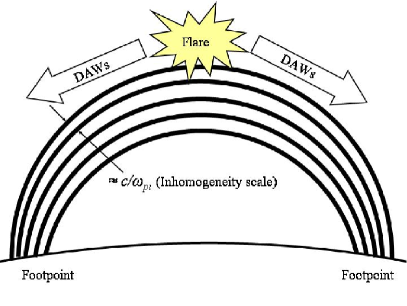
Figure 1: A conceptual sketch of the model. A solar flare launches DAWs from the solar coronal loop apex which rush down towards the photospheric footpoints, accelerating electrons along the propagation direction and heating ions in the transverse direction. The transverse inhomogeneity scale is $\approx 30$ Debye length ($\lambda_{D}$) that for the considered mass ratio $m_{i}/m_{e}=16$ corresponds to $0.75c/\omega_{pi}$.

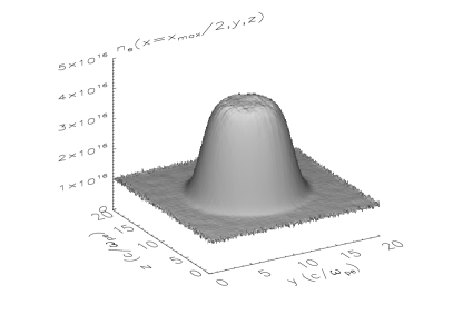
Figure 2: Shaded surface plot of $n_{e}(x=x_{m}/2,y,z)$ at $t=0$.

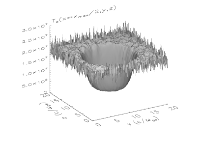
Figure 3: Shaded surface plot of $T_{e}(x=x_{m}/2,y,z)\propto 1/n_{e}(x=x_{m}/2,y,z)$ at $t=0$.

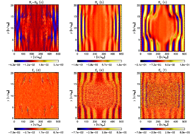
Figure 4: Contour (intensity) plots of the following physical quantities at $t_{end}=75\omega_{ci}^{-1}$: (a) $B_{x}(x,y,z=z_{m}/2)-B_{0}$, (b) $B_{y}(x,y,z=z_{m}/2)$, (c) $B_{z}(x,y,z=z_{m}/2)$, (d) $E_{x}(x,y,z=z_{m}/2)$, (e) $E_{y}(x,y,z=z_{m}/2)$, (f) $E_{z}(x,y,z=z_{m}/2)$. These correspond to a vertical cut through the mid-plane $z=z_{m}/2$.

Figure 5: Time evolution (at $t=0$ and $t=t_{end}=75\omega_{ci}^{-1}$) of electron and ion velocity distribution functions versus velocity $x,y$ and $z$ components on a log-linear plot: (a) $f_{e}(v_{x},t=0)$ dashed (inner) curve and $f_{e}(v_{x},t=t_{end})$ solid (outer) curve, (b) $f_{e}(v_{y},t=0)$ dashed (inner) curve and $f_{e}(v_{y},t=t_{end})$ solid (outer) curve, (c) $f_{e}(v_{z},t=0)$ dashed (inner) curve and $f_{e}(v_{z},t=t_{end})$ solid (outer) curve, (d) $f_{i}(v_{x},t=0)$ dashed (inner) curve and $f_{i}(v_{x},t=t_{end})$ solid (outer) curve, (e) $f_{i}(v_{y},t=0)$ dashed (inner) curve and $f_{i}(v_{y},t=t_{end})$ solid (outer) curve, (f) $f_{i}(v_{z},t=0)$ dashed (inner) curve and $f_{i}(v_{z},t=t_{end})$ solid (outer) curve. Time evolution (at 20 time intervals between $t=0$ and $t=t_{end}$) of the following: (g) $\max|E_{x}(x,y,z,t)|$, triangles connected with a solid curve and (h) $AH_{\parallel,e}(t)$ index, diamonds connected with dashed curve, according to Eq.(7), $AH_{\perp,i}(t)$ index, triangles connected with a solid curve, according to Eq.(8).

Figure 6: Time evolution (at $t=0$ and $t=t_{end}=75\omega_{ci}^{-1}$) of electron and ion velocity distribution functions (with positive velocities) versus kinetic energy of particles $E$ on a log-log plot. Top row: (a) $f_{e,Vx}(E,t=0)$ thin solid (inner) curve and $f_{e,Vx}(E,t=t_{end})$ thick solid (outer) curve, (b) $f_{e,Vy}(E,t=0)$ thin solid (inner) curve and $f_{e,Vy}(E,t=t_{end})$ thick solid (outer) curve, (c) $f_{e,Vz}(E,t=0)$ thin solid (inner) curve and $f_{e,Vz}(E,t=t_{end})$ thick solid (outer) curve. Vertical line in (a) corresponds to the kinetic energy, $E_{DAW}=(\gamma-1)m_{e}c^{2}$, with $\gamma=1/\sqrt{1-0.201^{2}}$ and $0.201c$ being phase velocity of left-hand polarised IAW in the low density region. Dotted line is $2\times 10^{10}E^{-1.5}$ and dashed line is $10^{7}E^{-4}$. Bottom row: (d) $f_{i,Vx}(E,t=0)$ thin solid (inner) curve and $f_{i,Vx}(E,t=t_{end})$ thick solid (outer) curve, (e) $f_{i,Vy}(E,t=0)$ thin solid (inner) curve and $f_{i,Vy}(E,t=t_{end})$ thick solid (outer) curve, (f) $f_{i,Vz}(E,t=0)$ thin solid (inner) curve and $f_{i,Vz}(E,t=t_{end})$ thick solid (outer) curve.

Figure 7: As in Fig. 6 but for run L16 from Ref.Tsiklauri (2011). Dotted line is $10^{9}E^{-2}$ and dashed line is $2\times 10^{3}E^{-6}$.

Figure 8: As in Fig. 6 but for run L73 from Ref.Tsiklauri (2011). Vertical line in (a) corresponds to the kinetic energy, $E_{DAW}=(\gamma-1)m_{e}c^{2}$, with $\gamma=1/\sqrt{1-0.097^{2}}$ and $0.097c$ being phase velocity of left-hand polarised IAW in the low density region. Dotted line is $10^{10}E^{-2}$ and dashed line is $10^{-1}E^{-8}$.

We consider a transverse to the background magnetic field variation of number density as following

$${n_{i}(y)}={n_{e}(y)}=$$

$$1+3\exp\Biggl{[}-\left(\frac{\sqrt{(y-y_{0})^{2}+(z-z_{0})^{2}}}{50\lambda_{D}}\right)^{6}\Biggl{]}=$$

$$1+3\exp\Biggl{[}-\left(\frac{|\vec{r}-\vec{r}_{0}|}{50\lambda_{D}}\right)^{6}\Biggl{]}\equiv f(y,z).$$ (1)

Eq.(1) implies that in the central region (across the $y$ and $z$ directions), the density is smoothly enhanced by a factor of 4, and there are the strongest density gradients having a width of about ${30\lambda_{D}}$ around the points $r_{s}=\sqrt{y^{2}+z^{2}}=51.5\lambda_{D}$ and $r_{s}=148.5\lambda_{D}$. Here $r_{0}=(y_{0},z_{0})=(100\lambda_{D},100\lambda_{D})$. Fig. 2 shows $n_{e}(x=x_{m}/2,y,z)$ at $t=0$, which indicates that the number density at the cylindrical tube centre increases by factor of 4 compared to the exterior. This density behaviour represents the solar coronal loop. The background temperature of ions and electrons are varied accordingly

$${T_{i}(y,z)}/{T_{0}}={T_{e}(y,z)}/{T_{0}}=f(y,z)^{-1},$$ (2)

such that the thermal pressure remains constant. Because the background magnetic field along the $x$-coordinate is constant, the total pressure is also constant. Fig. 3 shows $T_{e}(x=x_{m}/2,y,z)\propto 1/n_{e}(x=x_{m}/2,y,z)$ at $t=0$. Note how the temperature at the cylindrical tube centre decreases by factor of 4 compared to the exterior.

The DAW is launched by driving domain left edge, $x=1\lambda_{D}$, as follows

$$E_{y}(1,y,z,t+\Delta t)=E_{y}(1,y,z,t)-$$

$$A_{y}\sin(\omega_{d}t)\left(1-\exp\left[-(t/t_{0})^{2}\right]\right),$$ (3)

$$E_{z}(1,y,z,t+\Delta t)=E_{z}(1,y,z,t)-$$

$$A_{z}\cos(\omega_{d}t)\left(1-\exp\left[-(t/t_{0})^{2}\right]\right),$$ (4)

which produces the case of left-polarised DAW, i.e. ion cyclotron wave. $\omega_{d}$ denotes the driving frequency which was fixed at $\omega_{d}=0.3\omega_{ci}$. The fact that $\omega_{d}<\omega_{ci}$ ensures that no ion-cyclotron damping is present and also that the generated DAW is well on the Alfven wave branch with dispersion properties similar to the Alfven wave (cf. Fig. 3.4 from Ref.Dendy (2002)). $t_{0}$ is the onset time of the driver, which was fixed at $3.0\omega_{ci}^{-1}$ i.e. $48.000\omega_{pe}^{-1}$ for the case of $m_{i}/m_{e}=16$. Thus the driver onset time is $9\omega_{ci}^{-1}$ (9 comes from $3^{2}$). The initial amplitudes of the $E_{\perp}$ are chosen as $A_{y}=A_{z}=0.05(cB_{0x})$. Therefore magnetic perturbation amplitude of DAW is 5% of the background magnetic field, thus the simulation is weakly non-linear. Such transverse electric field $E_{\perp}=E_{y,z}$ driving generates L-circularly polarised DAW. For further details on polarisation see paragraph before Eq.(7) from Ref. Tsiklauri (2011). In the case of L-circularly polarised DAW the dispersion is

$$k=\frac{\omega}{c}\left(1+\frac{\omega_{pe}^{2}+\omega_{pi}^{2}}{(\omega_{ce}+\omega)(\omega_{ci}-\omega)}\right)^{1/2}.$$ (5)

Eq.(5) shows that when $\omega=\omega_{ci}$ the ion-cyclotron resonance occurs.

III Results

Fig. 4 presents the numerical simulation results for the electromagnetic fields. We see from Figs.4(e) and 4(f) that in response to the transverse electric field driving, which proceeds according to Eqs.(3) and (4), left-hand, circularly polarised IAW has developed three wavelength. If we use Eq.(5), then for the considered plasma parameters, $3\times(2\pi/k)/(c/\omega_{pe})=201.7$. We gather from Fig. 4(e) that the waveform at $y=0$ has travelled to $x\approx 200$. It has not reached $z=201.7$ quite yet because the driving onset time is $9\omega_{ci}^{-1}$. We see that $E_{y}$ component develops phase mixing i.e. waveform distorts across the transverse $y$ and $z$ coordinates generating strong transverse gradients. The transverse magnetic fields have similar behaviour to transverse electric fields. However, phase-mixed field component is $B_{z}$ (Fig. 4(c)). Movie that shows time dynamics of $B_{z}(x,y,z=z_{m}/2)$ (a plane that cuts through the middle of the over-dense tube, along the background magnetic field) is shown in the supplementary material mov . Fig. 4(d) shows that parallel electric field is generated only in the density inhomogeneity regions $4<r<7$ and $13<r<16$, where $r=\sqrt{y^{2}+z^{2}}$. The time evolution of this parallel electric field is shown in two different cross-sections in the supplementary material mov : $E_{x}(x,y,z=z_{m}/2)$ (a plane that cuts through the middle of the over-dense tube, along the background magnetic field) and $E_{x}(x=x_{m}/8,y,z)$ (a plane that cuts through the 1/8th of the over-dense tube, across the background magnetic field). We gather from movie 2 mov that in this 3D simulation, in the plane cut along the background magnetic field, behaviour is similar to 2.5D results both in PIC simulation (see e.g. Fig. 1 from Ref.Tsiklauri (2011)) or cold plasma approximation (see animation 2 (in Supplementary Data) from Ref.Tsiklauri (2007)). What is new in 3D is the ability to study the transverse structure of the parallel electric field. Somewhat unexpected results are shown in movie 3 mov . The bright yellow blob that can be seen rotating around the centre is a marker to guide ones eye. It rotates in the clockwise direction with the angular frequency of $0.3\omega_{ci}$. Its dynamics is described by the equation

$$marker(y,z,t)=2.0\times 10^{-2}\exp\Bigl{(}$$

$$-\bigl{\{}[(y-y_{m}/2)\cos(0.3\omega_{ci}t+\pi)-$$

$$(z-z_{m}/2)\sin(0.3\omega_{ci}t+\pi)-y_{m}/4]/0.5\bigr{\}}^{2}$$

$$-\bigl{\{}[(z-z_{m}/2)\cos(0.3\omega_{ci}t+\pi)+$$

$$(y-y_{m}/2)\sin(0.3\omega_{ci}t+\pi)-z_{m}/4]/0.5\bigr{\}}^{2}\Bigr{)}.$$ (6)

We see only the marker blob rotating in the clockwise direction until about time $t\leq 600\omega_{pe}$. Then the generated parallel electric field reaches the plane corresponding to $x=x_{m}/8$ in which this movie is produced. From $t\geq 600\omega_{pe}$ until the end of the simulation we see that parallel electric field is localised within circular bands $4<r<7$ and $13<r<16$ and rotating in the clockwise direction with the frequency $0.3\omega_{ci}$. This seems initially surprising why the parallel electric field should rotate. However, if one recalls that the IAW also rotates in the same clockwise direction, then this seems logical (that both parts of the wave $E_{\perp}$ that is used as a driver and the generated $E_{\parallel}$ both rotate in the same sense and with same angular frequency). Note that rotation in movie 3 and translatory motion in movies 1 and 2 mov appear step-like because there are only 20 time snapshots taken throughout the simulation that ends at $t_{end}=75\omega_{ci}^{-1}=1200\omega_{pe}^{-1}$. Thus in this animation $\Delta t=3.75\omega_{ci}^{-1}$. Also, in all movies distances on $x-y$ axes are quoted in number of grid points – not in $c/\omega_{pe}$ as in the rest of the paper. Thus, the conclusion here is that the generated parallel electric field is localised in the density inhomogeneity region and rotates in the same direction and with the same angular frequency as the initially launched DAW.

We quantify the particle acceleration and plasma heating by defining the following indexes:

$$AH_{\parallel,e}(t)=$$

$$\frac{\int_{|v_{x}|>\langle v_{th,e}\rangle}^{\infty}f_{e}(v_{x},t)dv_{x}\bigl{/}\left(x_{m}\pi[(r_{o}-r_{0})^{2}-(r_{i}-r_{0})^{2}]\right)}{\int_{-\infty}^{\infty}f_{e}(v_{x},0)dv_{x}\bigl{/}\left(x_{m}y_{m}z_{m}\right)},$$ (7)

$$AH_{\perp,i}(t)=$$

$$\frac{\int_{|v_{\perp}|>\langle v_{th,i}\rangle}^{\infty}f_{i}(v_{\perp},t)dv_{\perp}\bigl{/}\left(x_{m}\pi[(r_{o}-r_{0})^{2}-(r_{i}-r_{0})^{2}]\right)}{\int_{-\infty}^{\infty}f_{i}(v_{\perp},0)dv_{\perp}\bigl{/}\left(x_{m}y_{m}z_{m}\right)},$$ (8)

where $r_{o}$ and $r_{i}$ are outer and inner radii of the density inhomogeneity shown in Fig. 2 and $r_{0}$ is its mid-point (centre). $f_{e,i}$ are electron or ion velocity distribution functions. They are normalised in such a way that when integrated by all spatial and velocity components they give the total number of real electrons and ions (not pseudo-particles that usually mimic much larger number of real particles in the PIC simulation). The definition used in Eq.(7) effectively provides the fraction (the percentage) of accelerated electrons, parallel to the magnetic field, in the density gradient regions. Eq.(8) gives the fraction (the percentage) of heated ions, perpendicular to the magnetic field. In the case of 2.5D similar indexes have been defined in Ref.Tsiklauri (2011). We refer interested reader for an underlying discussion of these indexes in the former reference. We gather from Fig. 5(a)–5(c) that electron acceleration is confined only to the parallel to the background magnetic field direction. This can be evidenced by appearance of the bumps in the $f_{e}(v_{x})$ at $t=t_{end}$, which correspond to the electron beams produced by the generated $E_{x}=E_{\parallel}$ in the density inhomogeneity. By comparing Fig. 5(a) (electrons) with Fig. 5(d) (ions) we see that no ion beams are generated. Instead we see from Figs. 5(e) and 5(f) that ions are heated in the perpendicular direction as the distribution function at $t=t_{end}$ widens (whilst no ion beams are produced). Note that such transverse ion heating of plasma has been studied in the past too Chaston et al. (2004); Voitenko and Goossens (2004); Wu and Yang (2006, 2007), while the main focus here is the electron acceleration in the parallel direction. Comparing Fig. 5(a) (electrons) with Fig. 5(d) (ions) also gives us an indication that because in the density gradient region (circular ring) ions essentially do not feel IAW driving in the parallel direction while electrons are accelerated, effective charge separation takes place. This is consistent with the cold plasma approximation, see animation 3 (in Supplementary Data) from Ref.Tsiklauri (2007). We gather from Fig. 5(g) that the value of the generated parallel electric field, in normalised units, is 0.07. It can be also seen from Fig.5(h) that $AH_{\parallel,e}(t)$ and $AH_{\perp,i}(t)$ indexes attain values of 0.45 (45%) and 0.75 (75%) respectively. Fig. 3 from Ref.Tsiklauri (2011) directly corresponds to our Fig. 5 here but now for the 3D case. Thus we can make some comparisons. The differences are: (i) in 3D case parallel electron beams are more pronounced, as the solid line in Fig. 5(a) attains higher values also over the larger $v_{x}$ range. (ii) in 3D case the transverse ion heating is more pronounced too, as the solid lines in Figs. 5(e) and 5(f) reach higher values compared to the 2.5D case. (iii) in 3D case parallel electric field attains values roughly a factor of two larger, as Fig. 5(g) shows that the value of the parallel electric field attains 0.07 versus 0.03 in the 2.5D case. (iv) the fraction of accelerated electrons, parallel to the magnetic field, in the density inhomogeneity is factor of two larger, as it can be seen from Fig. 5(h) that $AH_{\parallel,e}(t_{end})=0.45$ versus $AH_{\parallel,e}(t_{end})=0.2$ in the 2.5D case and the fraction of heated ions, perpendicular to the magnetic field, is also factor of two larger, as it can be seen from Fig. 5(h) that $AH_{\perp,i}(t_{end})=0.75$ versus $AH_{\perp,i}(t_{end})=0.35$ in the 2.5D case.

Fig. 6 presents the same data in panels (a)–(f) from Fig. 5 but now in terms of kinetic energy $E=(\gamma-1)m_{e}c^{2}$ and also plotted on the log-log plot. Note that in Fig. 5 log-normal plot was used. To produce Fig. 6 only $v_{x}>0$ branch was used. The reason for producing Fig. 6 is two-fold: (i) to demonstrate that the electron spectrum in the parallel to the field direction shows so-called ”knee” – a break in the spectra power-laws; (ii) to demonstrate that the ”knee” can be interpreted is the Landau damping (Cerenkov resonance effect) due to the wave-particle interactions. There are several explanations for the observed double power-laws in the electron spectrum. By double we mean one (usually smaller $\propto E^{-\alpha}$ with $2<\alpha<4$) power-law index below a certain fixed energy $E<E_{br}$ (where 50 keV $<E_{br}<$ 150 keV and then another (usually larger $\propto E^{-\alpha}$ with $4<\alpha<7$) power-law index for $E>E_{br}$ Dulk et al. (1992). Chapter 13.3.4 of Ref.Aschwanden (2005) quotes several explanations for the double power-law also known as the ”knee”. The most common explanation is collisional relaxation of an electron beam, with added refinements such as the generation of Langmuir waves and plasma density inhomogeneity Kontar et al. (2012). Here we offer an alternative explanation in that flare generated DAWs produce electron beams on the transverse density inhomogeneities (magnetic loop edges) which in turn produce spectra with the structure that resembles the knee.

Fig. 7 is analogous to Fig. 6 but it has been produced with the simulation data from run L16 from Ref.Tsiklauri (2011) that corresponds to 2.5D. Comparison of Fig. 7 (2.5D case, Ref.Tsiklauri (2011)) and Fig. 6 (3D case, this paper) enables to grasp the differences between 2.5D and 3D geometry. It is evident from Figs. 7 and 6 that in the 3D case acceleration of electrons along the magnetic field and heating of ions in the transverse direction is more efficient. Also, the knee feature in the parallel to the magnetic field electron spectra can be seen.

Fig. 8 is analogous to Fig. 6 but it has been produced with the simulation data from run L73 from Ref.Tsiklauri (2011) that corresponds to 2.5D. Comparison of Fig. 8 (2.5D case, Ref.Tsiklauri (2011) mass ratio $m_{i}/m_{e}=73.44$), Fig. 7 (2.5D case, Ref.Tsiklauri (2011) mass ratio $m_{i}/m_{e}=16$) and Fig. 6 (3D case, this paper, mass ratio $m_{i}/m_{e}=16$) enables to gauge the differences between 2.5D versus 3D geometry as well as one mass ratio versus another (note that considered mass ratios land the physical system into different regimes. Case of $m_{i}/m_{e}=16$ corresponds to IAW regime, whereas $m_{i}/m_{e}=73.44$ corresponds to KAW regime). We gather from Fig. 8 that double power-law fit to the parallel electron spectrum is better compared to Figs. 7 and 6, possibly indicating that the KAW regime provides more double power-law-like behaviour. It should be noted that in Fig. 7 and 6 corresponding to IAW regime power-law fit seems somewhat arbitrary. This partly could also be due to the fact that the observations usually provide time-averaged electron spectrum whereas no-time averaging has been used in Figs.6–8. A more profound result is that the energy, $E_{DAW}$, that corresponds to the break in the power-law, $E_{br}$, approximately corresponds the energy of an electron which moves with the phase speed of the DAW, $V_{ph}$. In other words we note that as we increase the mass ratio from 16 to 73.44 both the break in the spectrum and $V_{ph}$ decrease. This demonstrates that the ”knee” can possibly be interpreted as the Landau damping (Cerenkov resonance effect) of DAWs due to the wave-particle interactions.

IV Conclusions

The aim of this work was to explore the novelties brought about by 3D geometry effects into the problem of particle acceleration by DAWs in the solar flare and also to Earth magnetosphere auroral zone studied in an earlier 2.5D geometry work Tsiklauri (2011). It should be noted that here we have studied the case of plasma over-density, transverse to the background magnetic field, whereas references that deal with Earth auroral zone usually consider the case of plasma under-density (a cavity), as dictated by the different applications considered (solar coronal loops and Earth auroral plasma cavities). As far as the generation of parallel electric field and associated particle acceleration is concerned, there is no difference whether the transverse density gradient is positive or negative – for the mechanism to work it has to be non-zero. This is because whistlers (and ion cyclotron waves) that propagate strictly along the magnetic field display no Landau damping, since the longitudinal component of the wave electric field is zero Stepanov et al. (2012), page 124. The latter becomes non-zero as the wave front turns due to the transverse density inhomogeneity. Thus we investigated a process of particle acceleration by left-hand, circularly polarised inertial Alfven wave in a transversely inhomogeneous plasma, using 3D particle-in-cell simulation. We considered a cylindrical tube that contains a transverse to the background magnetic field inhomogeneity with a scale of the order of ion inertial length. Such numerical setup is relevant for solar flaring loops and earth auroral zone. In such structure IAWs with frequency $0.3\omega_{ci}$ were launched and allowed to develop three wavelength. The following key points have been established: Propagation of IAW in such a system generates time-varying parallel electric field, localised in the density gradient regions, which accelerate electrons in the parallel to magnetic field direction. Perpendicular electric field of IAW also effectively heats ions in the transverse direction. The generated parallel electric field rotates in the same direction and frequency as the ”parent” IAW. The fully 3D kinetic simulation demonstrates electron acceleration efficiency in the density inhomogeneity regions, along the magnetic field, is of the order of 45% and ion heating, in the transverse to the magnetic field direction, is about 75%. The latter is a factor of two times higher than the previous 2.5D analogous study and is broadly in agreement with the solar flare particle acceleration observations. Log-log plots of electron spectra seem to indicate that the ”knee”, frequently seen in the solar flare observations, can be interpreted is the Landau damping of IAWs due to the wave-particle interactions.