Simultaneous Reduction of Two Common Autocalibration Errors in GRAPPA EPI Time Series Data

Abstract

The GRAPPA (GeneRalized Autocalibrating Partially Parallel Acquisitions) method of parallel MRI makes use of an autocalibration scan (ACS) to determine a set of synthesis coefficients to be used in the image reconstruction. For EPI time series the ACS data is usually acquired once prior to the time series. In this case the interleaved $R$-shot EPI trajectory, where $R$ is the GRAPPA reduction factor, offers advantages which we justify from a theoretical and experimental perspective. Unfortunately, interleaved $R$-shot ACS can be corrupted due to perturbations to the signal (such as direct and indirect motion effects) occurring between the shots, and these perturbations may lead to artifacts in GRAPPA-reconstructed images. Consequently we also present a method of acquiring interleaved ACS data in a manner which can reduce the effects of inter-shot signal perturbations. This method makes use of the phase correction data, conveniently a part of many standard EPI sequences, to assess the signal perturbations between the segments of $R$-shot EPI ACS scans. The phase correction scans serve as navigator echoes, or more accurately a perturbation-sensitive signal, to which a root-mean-square deviation perturbation metric is applied for the determination of the best available complete ACS data set among multiple complete sets of ACS data acquired prior to the EPI time series. This best set (assumed to be that with the smallest valued perturbation metric) is used in the GRAPPA autocalibration algorithm, thereby permitting considerable improvement in both image quality and temporal signal-to-noise ratio of the subsequent EPI time series at the expense of a small increase in overall acquisition time.

1 Introduction

Parallel accelerated MRI (Sodickson and Manning, 1997; Jakob et al., 1998; Pruessmann et al., 1999; Griswold et al., 2002) increases image acquisition speed by using the spatial sensitivity of each receiver coil in an array of receiver coils, in addition to the spatial encoding provided by the applied linear magnetic field gradients used in conventional (non-accelerated) imaging. Relative to conventional imaging this additional spatial information allows one to reduce the number of acquired phase-encoded (PE) lines of data, while maintaining a desired digital resolution and field-of-view (FOV), thereby accelerating the data acquisition. This increase in the image acquisition speed is usually stated in terms of the reduction factor $R$ which is defined, for fixed nominal digital image resolution and FOV, as the ratio of the number of acquired PE lines for a conventional scan to the number of acquired PE lines for a parallel accelerated imaging scan.

For the sake of clarity we make some definitions before continuing with this introduction. In keeping with terminology initiated in Griswold et al. (Griswold et al., 2002) we will refer to the data sampled during accelerated imaging as the reduced set of PE lines and we will refer to the PE lines which are absent from the parallel accelerated imaging data set, but present in a conventional data set, as the missing set of PE lines. In addition we will refer to the union of the reduced set and the missing set as the nominal set of PE lines - equivalent to the set of PE lines acquired during conventional imaging - since it is the sampling characteristics of this set which determine the nominal digital image resolution and FOV. The right-hand side of Figure 1 and the lower part of Figure 2 illustrate these definitions as they pertain to an EPI time series.

Figure 1: 1-shot ACS acquisition: This figure illustrates the ACS and time series k-space data associated with a single 2D image slice for the $R=3$ case. The bold arrow indicates temporal order of acquisition and the ${\bigtimes}$ symbol denotes multiple acquisitions of the data contained within the vertical square brackets. The solid horizontal lines in k-space denote the acquired data. A complete set of ACS data consists of $N_{a}$ PE lines which are collected during 1-shot EPI acquisition. In the time series data the reduced set and the missing set of PE lines are respectively denoted by the solid and dashed lines. There are $N_{s}$ PE lines in the nominal set of PE lines (nominal matrix size: $N_{s}\times N_{s}$).

The GRAPPA method of parallel imaging (Griswold et al., 2002) has been of great interest since, unlike other parallel imaging methods such as SENSE (Sensitivity Encoding) (Pruessmann et al., 1999), it does not require explicit knowledge of the receive fields for each element of the receiver array. Instead, the GRAPPA method uses the data from the receiver array in an autocalibration procedure which estimates a set of synthesis coefficients used to synthesize the missing set of PE lines from the reduced set of PE lines over the set of receiver coils. Central to the autocalibration procedure is the acquisition of autocalibration scan (ACS) data consisting of a subset of the nominal set of PE lines. This subset, comprised of PE lines near the center of k-space, will be referred to as the complete set of ACS data. This complete ACS data set is used to calculate the synthesis coefficients over the set of receiver array channels. The left-hand side of Figure 1 and the upper part Figure 2 illustrate these definitions as they pertain to $N_{a}$ PE lines of a complete ACS data set acquired prior to an EPI time series for $1$-shot and $R$-shot interleaved ACS, respectively.

Figure 2: R-shot segmented ACS acquisition: This figure illustrates the ACS and time series k-space data associated with a single 2D image slice for the $R=3$ case. The bold arrows indicate temporal order of acquisition and the $\bigtimes$ symbol denotes multiple acquisitions of the data contained within the vertical square brackets. The solid horizontal lines in k-space denote the acquired data. A complete set of ACS data consists of $N_{a}$ PE lines which are collected during $R$ shots of a segmented EPI acquisition. In the time series data the reduced set and the missing set of PE lines are respectively denoted by the solid and dashed lines. There are $N_{s}$ PE lines in the nominal set of PE lines (nominal matrix size: $N_{s}\times N_{s}$).

For GRAPPA EPI time series the ACS data is usually collected once prior to the acquisition of the time series data (Schmiedeskamp et al., 2010). Both $1$-shot and $R$-shot interleaved $k$-space trajectories (Schmiedeskamp et al., 2010) have been used to acquire a complete set of ACS data. Figures 1 and 2 depict the k-space trajectories for $1$-shot and $R$-shot interleaved segmented acquisition respectively, of complete ACS data sets for the $R=3$ case. The justification for the use of the $R$-shot as opposed to the $1$-shot trajectory has not been clearly established in the literature, nor has a robust method been established for dealing with the potential consequences of inter-shot signal perturbations (such as motion) during acquisition of a complete $R$-shot ACS data set.

The intent of this paper is two-fold: (1) To justify the use of the $R$-shot interleaved EPI trajectory instead of the $1$-shot trajectory from a theoretical and experimental perspective when in the presence of significant main magnetic field inhomogeneity, and (2) To demonstrate a method of acquiring the $R$-shot interleaved EPI ACS data which minimizes potential artifacts due to signal perturbations occurring between the $R$ shots. We will not attempt to answer the question of under what circumstances (main field strength, susceptibility differences, FOV choice, and reduction factor) the artifact from motion may be greater than that from trajectory incompatibility. Our hope is that with refinement of the method presented here this trade-off will simply not be in question.

Although in this paper we focus on the direct effects of head motion - because we can control it to some extent - we note that ACS data acquired in a segmented manner can potentially be contaminated by any perturbation to the data that occurs on a timescale smaller than that required to sample a complete ACS data set. Such perturbations may include, for example, motion effects such as $B_{0}$ changes due to subject chest motion, magnetic susceptibility changes due to motion, perturbations to the time series steady-state when through-slice-plane motion occurs and signal spiking due to electrostatic discharge between cables.

We note that motion can perturb GRAPPA EPI time series data by two means: (1) Motion during the ACS data acquisition can lead to an inaccurate estimation of the synthesis coefficients, thereby leading to artifacts in all images of the time series along with a potential degradation of tSNR (temporal signal-to-noise ratio); and (2) Motion between the time of the ACS data acquisition and the time at which any particular image of the time series is acquired may make the synthesis coefficients inappropriate since the imaged object may have moved into regions where insufficient signal existed during the ACS data acquisition - an incomplete spatial sampling.

Cheng (Cheng, 2010) has investigated the use of TGRAPPA (Breuer et al., 2005), a method not yet commercially available, to provide new ACS lines for each volume of an EPI time series. This has the benefit of providing motion-uncontaminated ACS throughout the time series, but comes at the expense of reducing tSNR in the absence of significant subject motion, compared to the performance of GRAPPA. Thus, for fMRI applications, it is to be expected that GRAPPA would be preferable to TGRAPPA, provided GRAPPA can be made more robust to motion.

One of the methods in this paper involves assessing motion contamination of ACS data by the use of a navigator echo (Ehman and Felmlee, 1989) and a perturbation metric. Other investigators have studied methods by which to assess and reduce motion contamination of MRI data albeit in applications other than GRAPPA EPI time series. For example, Kim and Hu have used navigator echoes to limit the effects of motion in fMRI studies using the FLASH sequence (Hu and Kim, 1994) and the interleaved EPI sequence (Kim et al., 1996). 2D navigators have been used in conjunction with read-out segmented EPI (Heidemann et al., 2010) (Nguyen et al., 1998) for diffusion imaging, the navigator being used to determine whether a particular diffusion weighted image should be re-acquired due to motion contamination. Holdsworth et. al. (Holdsworth et al., 2009) have also used a k-space entropy metric to assess motion corruption in read-out segmented EPI for diffusion-weighted imaging. Law et. al. (Law et al., 2008) used a sliding window approach to update the coil sensitivity maps for the TSENSE (adaptive SENSE incorporating temporal filtering) (Kellman et al., 2001) method. Here we extend the application of navigator echoes to assessing motion between ACS segments, a direct extension of previous ideas, albeit with a new application.

The method presented here makes use of multiple $R$-shot interleaved ACS EPI data sets and phase correction echoes, which are already part of most commercial EPI sequences, to assess the motion between ACS EPI segments and produce a complete set of ACS EPI data that is minimally corrupted by motion. The phase correction echoes are therefore doing double-duty for they will be used in their usual capacity to eliminate Nyquist ghosting and they will be used as navigator echoes to assess motion. This complete set of ACS segments, assessed to be minimally contaminated by motion, is then used to estimate the GRAPPA synthesis coefficients and hence synthesize the missing PE lines for the entire time series. With this redundant ACS scheme, $R$-shot accelerated EPI time series can potentially be reconstructed with less artifact and greater tSNR in the presence of motion. This suggests improvements for fMRI applications which we evaluate with a simple measurement of tSNR.

2 Theory

In the GRAPPA method (Griswold et al., 2002) the missing set of PE lines, of a nominal set with inter-sample distance $\Delta k_{y}=1/{\rm FOV}$ in the PE direction, are synthesized according to the following equation:

$$S_{n}(m+r,x)=\sum_{n^{\prime}=1}^{N_{c}}\sum_{m^{\prime}=-b}^{b}S_{n}^{\prime}(m+m^{\prime}R,x)W_{nn^{\prime}m^{\prime}r}$$ (1)

where $R$ is the reduction factor, $m=\ldots-2R,-R,0,R,2R,\ldots$ enumerates the reduced set of PE lines, $r=1,\ldots,R-1$ is a PE offset from a PE line of the reduced set to a neighboring PE line of the missing set, $N_{c}$ is the number of coil elements in the receiver array, $W_{nn^{\prime}m^{\prime}r}(\tau_{y})$ are the synthesis coefficients and $b$ fixes a finite number of local PE lines of the reduced set to be used in the synthesis of the missing PE lines. Equation 1 is used in conjunction with the sampled ACS lines to perform an autocalibration step by which one obtains the synthesis coefficients through a fitting algorithm. Once the coefficients $W_{nn^{\prime}m^{\prime}r}$ are determined then Equation 1 is used to synthesize the missing set of PE lines from the reduced set of PE lines for each receiver coil. The images for each coil are then reconstructed by a simple FFT (Fast Fourier Transform) of the nominal set of PE lines, followed by a square-root of a sum-of-squares combination (Roemer et al., 1990; Larsson et al., 2003) of the individual coil images to produce the final image.

The number of ACS lines $N_{a}$ (see Figures 1 and 2) is usually significantly smaller than the nominal size $N_{s}$ of the sampling matrix in the PE direction. For non-EPI imaging sequences the ACS data and the reduced data can usually be acquired together by adding a few additional k-space lines (for ACS) to the sequence. This method of collecting ACS data is usually considered unacceptable for EPI time series because it would extend the echo train length significantly and require unacceptable compensatory adjustments to the image-space spatio-temporal sampling, and because it would exacerbate the EPI-inherent effect of geometric distortion due to main field inhomogeneity. Therefore, for GRAPPA EPI time series the ACS are usually acquired once prior to the time series and a single estimation of the synthesis coefficients is done followed by repeated calculations of the missing PE lines from the reduced data sets at each discrete time point $n$ of the time series.

There is some flexibility in the scheme used to acquire ACS for an EPI time series. For $R$-fold acceleration it is possible to use 1-shot to $R$-shot (interleaved) ACS trajectories, each with distinct advantages and caveats. For example, a rapid estimation of GRAPPA coefficients may be obtained with a $1$-shot ACS (see Figure 1), using $\Delta k$ matched to that of the nominal set of PE lines (Porter and Heidemann, 2009; Heidemann et al., 2010). This ACS data set should be relatively uncontaminated by sample motion during the ACS acquisition itself. However, the $R$-shot trajectory (see Figure 2) has the advantage of eliminating artifact that results when the signal dynamics over a $1$-shot ACS sampling trajectory differ significantly from that over the reduced data set trajectory, as may occur in the presence of main field inhomogeneity (Cheng, 2010) or $T_{2}^{*}$ signal relaxation. A shows, from a mathematical frames perspective, that the GRAPPA equations are expected to break down when significant main magnetic field inhomogeneity is present unless the ACS data is acquired in a matched $R$-shot trajectory. This breakdown of the GRAPPA equations is expected to be exacerbated when using strong main fields since main field inhomogeneity increases with main field strength and since a large reduction factor is often used to control the resulting geometric distortions due to the field inhomogeneity.

In the remainder of this paper we: (1) Demonstrate the effects of ACS trajectories unmatched with respect to field inhomogeneity perturbations and $T_{2}^{*}$ signal relaxation; and (2) Propose and demonstrate a simple method by which residual aliasing due to motion between $R$-shot ACS segments may be reduced. The phase correction lines (see Figure 3) which precede each 2D slice in commercial EPI sequences are used as navigator echoes to assess whether signal changes due to motion or other perturbations have occurred between the segments of a complete ACS data set. Using the data from these navigator echoes the following metric $M_{s}$ will be used to assess the perturbations between the $R$ segments of the $s^{th}$ complete ACS data set:

$$M_{s}=\sqrt{\frac{\sum_{m=1}^{N_{c}}\sum_{n=1}^{N_{s}}\sum_{j=1}^{R-1}||S_{sjm}[n]-S_{s,j+1,m}[n]||^{2}}{\sum_{m=1}^{N_{c}}\sum_{n=1}^{N_{s}}||S_{s1m}[n]||^{2}}}$$ (2)

where $S_{sjm}[n]$, $j$, $m$ and $n$ are the FFT of a line of phase correction data, the segment index ($j=1,\ldots,R$), the coil element index and the sampling index in the frequency-encoding direction, respectively. We expect that complete ACS data sets with the smallest associated $M_{s}$ will produce EPI images with the least residual aliasing.

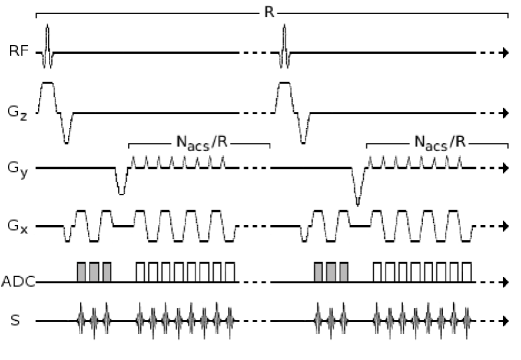
Figure 3: Sequence diagram for the acquisition of one complete set of ACS data. $G_{x}$, $G_{y}$ and $G_{z}$ denote the frequency-encoding, phase-encoding and slicing gradients respectively. The gray-filled ADC regions identify the phase correction data lines which were also used as navigator echoes to detect motion between interleaved ACS segments. Note that the prephasing $G_{y}$ gradient is incremented for each ACS segment to achieve the interleaving.

3 Methods

A single phantom experiment was performed to demonstrate the artifacts encountered when the $1$-shot ACS trajectory is used in the presence of significant main field inhomogeneity. Two brain experiments were performed to show the efficacy of the proposed navigator-based method of acquiring ACS with reduced motion contamination.

3.1 Data Acquisition

All data were acquired on a Siemens TIM Trio 3T whole-body scanner with a $12$-channel phased array head receiver coil. Brain images were obtained from volunteers in accordance with a protocol approved by the institutional Committee for the Protection of Human Subjects.

3.1.1 Phantom Experiment

In the first experiment we acquired data to compare GRAPPA reconstructed EPI images resulting from $R$-shot segmented interleaved ACS versus $1$-shot ACS. A structural phantom (The Phantom Lab, Salem, NY, USA) was used to assure that the image data was motion-free. An EPI sequence was modified in-house to either acquire ACS data for $R=3$ GRAPPA in a $1$-shot acquisition or a segmented interleaved $3$-shot acquisition. It should be noted that Siemens’ commercial sequences use a $1$-shot trajectory for $R=2$ and an $R$-shot segmented interleaved trajectory for $R>2$ when acquiring the ACS data set.

The relevant imaging parameters for this comparison were as follows: TR = $2450$ ms, TE = $33$ ms, nominal matrix size $N_{s}\times N_{s}$ = $96\times 96$, FOV = $224\times 224$ mm, number of ACS reference lines $N_{a}$ = $24$, echo-spacing = $1.6$ ms and slice thickness = $3$ mm. This experiment facilitated an evaluation of the potential for mismatched field inhomogeneity to affect residual aliasing. Note that an echo spacing roughly twice as long as is typical for fMRI was chosen to provide a clear example of the mismatch problem. We did not set out to evaluate the severity of the artifact for $1$-shot $R$-fold acceleration per se.

3.1.2 Brain Experiments

In a second experiment we demonstrate the proposed method of multiple ACS acquisition for eliminating residual aliasing due to motion during $R$-shot ACS. Multislice 2D brain images were obtained from volunteers using the following imaging parameters: GRAPPA with $R=2$, echo-spacing = $0.8$ ms, nominal matrix size $N_{s}\times N_{s}$ = $64\times 64$, number of phase correction reference scans (which also serve as the navigator echoes) = $3$, and TR = $2000$ ms. An EPI sequence was modified in-house to acquire $N_{acs}=10$ complete $R=2$ interleaved ACS data sets (see Figure 2 for a depiction of the analogous $R=3$ case) instead of the usual single complete set. Each interleaved ACS EPI segment acquired $12$ PE lines for a total of $24$ ACS lines ($N_{a}=24$) in a complete ACS data set. Following the ACS acquisition a single volume of 2D multislice image data (the reduced set) was acquired. For fMRI applications a time series of reduced data volumes would be acquired, but in this experiment we were only interested in the effects of motion during the ACS and therefore a single reduced k-space volume was sufficient.

In order to investigate the various effects of subject motion during interleaved ACS, four separate trials were acquired in the second experiment. During the acquisition of the first three trials the subject nodded their head (approximately 3 degrees) in randomly distributed $4$-second intervals, between which the subject tried to remain motionless. During the acquisition of the fourth trial the subject tried to remain motionless throughout the acquisition of the $10$ complete ACS data sets. The fourth trial was considered to be the target, or ”best case”, data.

In a third experiment we sought to assess the effect of motion contaminated ACS on the tSNR of a time series EPI acquisition, as would be used for fMRI. Once, again the subject was instructed to nod their head during ACS acquisition after which they were to remain motionless throughout an EPI time series. The relevant imaging parameters were $R$ = $2$, number of time series volumes $N_{epi}$ = $100$, nominal matrix size $N_{s}\times N_{s}$ = $64\times 64$, number of ACS reference lines $N_{a}$ = $24$, number of repetitions of segmented interleaved ACS complete data set $N_{acs}=10$ (as depicted in Figure 2), number of phase correction reference scans (which also serve as the navigator echoes) = $3$, TR = $2000$, TE = $28$ ms, echo-spacing = $0.52$ ms and FOV = $224$ mm.

3.2 Image Reconstruction

Image reconstruction was performed with either commercial Siemens GRAPPA algorithms and code or with in-house GRAPPA reconstruction code which implemented ”method 1” (a PE-only GRAPPA interpolation with a small number of blocks and no sliding window averaging) given in Brau et al. (2008).

3.2.1 Phantom Experiment

For the first experiment image reconstruction was done on the scanner with standard Siemens reconstruction code for both the product and modified sequence.

3.2.2 Brain Experiments

For the second and third experiments the image reconstruction was done with in-house GRAPPA code. The EPI sequence acquires three phase correction lines prior to each 2D slice of image data which we used as navigator echoes. Using Eq. 2 we calculate $M_{s}$ associated with each phase correction line and then we simply averaged the three $M_{s}$ values to yield the final $M_{s}$ value for each of the complete ACS data sets of a given trial.

The four trials of the second experiment were processed in the manner of four ”ACS time series” acquisitions, with each set of the ten interleaved ACS being combined with the single reduced EPI data set following each looped ACS. The $20$ separate ACS segments from ten interleaved $R=2$ ACS acquisitions can be grouped into 19 complete ACS data sets using adjacent pairs only. We do not expect the order of the interleaved ACS acquisition to matter, but we chose to restrict the metric $M_{s}$ to ACS pairs acquired as nearest neighbor pairs in order to minimize motion and scanner drift effects. From each complete ACS data set the synthesis coefficients were estimated. The missing set of PE lines was then synthesized using the reduced data set of PE lines and the synthesis coefficients corresponding to each of the $N_{acs}=19$ complete ACS sets. This was done for each of the twelve coil elements, after which the data was Fourier transformed to image-space and the images from each coil were combined in a final sum-of-squares magnitude image.

Data from the third experiment was processed in two ways. As in the second experiment, $M_{s}$ was evaluated for 19 nearest neighbor pairs of complete ACS data sets from the 10 acquired ACS pairs. From these, the ACS pairs with the highest and lowest $M_{s}$ were determined and used in the reconstruction of the same $N_{epi}=100$ volume time series EPI data, from which tSNR maps were produced. TSNR images were obtained by calculating the ratio of the temporal mean to the temporal standard deviation over the EPI time series for each pixel in image space.

4 Results

4.1 Phantom Experiment

The bottom of row of Figure 4 shows, for the case of $R=3$, an example of the residual aliasing artifact that may result when $1$-shot ACS data is used to autocalibrate the synthesis coefficients. Such artifact is clearly undesirable and is much reduced by using $3$-shot segmented interleaved ACS instead, as shown in the top row of Figure 4. We did not seek to quantify the extent of residual aliasing because the amount depends on $R$, the main field inhomogeneity (which itself may depend upon main field strength and the heterogeneity of the magnetic susceptibility of the imaged object), echo-spacing time and the FOV. The effects of field inhomogeneity upon the GRAPPA equations are considered in A.

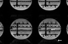
Figure 4: Top row: Five successive slices of $R=3$ GRAPPA images reconstructed using a 3-shot interleaved ACS data acquisition. Bottom row: The same set of image slices but using a single-shot ACS data acquisition. Note the residual aliasing (white arrows) which extends throughout the images of the bottom row. Exterior to the phantom the residual aliasing appears as misplaced image intensity, while interior to the phantom the residual aliasing appears as both increased and decreased local image intensity.

4.2 Brain Experiments

Figures 5 and 6 show the results for a GRAPPA-EPI $R=2$ acquisition acquired in the second experiment. Figure 5 shows plots of the perturbation metric $M_{s}$ associated with each of the 19 complete ACS data sets for the four motion trials. Although the perturbation metric in the first three trials attains values nearly an order of magnitude greater than those of the fourth (no intentional motion) trial, it is clear that low $M_{s}$ sets of ACS data are available in all cases.

Figure 6 shows the EPI images associated with successive complete ACS data sets. For brevity only the $10$ images associated with the even valued complete ACS data sets are shown, rather than all $19$. Image rows 1 through 4 correspond to the four different trials during which varying amounts of motion were introduced. Image row 4 was acquired as the subject tried to remain motionless throughout ACS acquisition. For each of the runs, the dashed boxes enclose the GRAPPA reconstructed images for which $M_{s}$ was highest and the solid boxes enclose the images for which $M_{s}$ was lowest. In each of the enclosed images the value of $M_{s}$ is given in the upper left corner. Figures 5 and 6 show a clear correlation between the perturbation metric $M_{s}$ and the visually apparent residual aliasing.

Figure 7 shows two mosaics of tSNR images for the same 100 volume EPI time series data acquired in the third experiment. The top mosaic is associated with the largest valued perturbation metric during the ACS while the bottom mosaic is associated with the smallest valued perturbation metric.

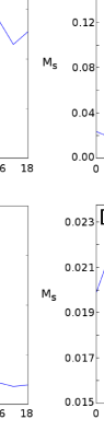
Figure 5: Plots of the perturbation metric $M_{s}$ as a function of the $n^{th}$ complete ACS data set. Plots A through D correspond respectively to rows 1 through 4 of Figure 6. Note that the scale of the ordinate varies between the four plots.

metric. Both images were constructed using the same gray-value scale. Visual inspection of these images shows significant improvement in tSNR of the EPI time series when the ACS data associated with the smallest valued perturbation metric is used in the calculation of the GRAPPA synthesis coefficients. For reference note that for the $5\times 5$ pixel region shown in Figure 7 the ratio of the mean tSNR for the largest valued metric case to the mean tSNR for smallest valued metric case is $tSNR_{smallest}/tSNR_{largest}=1.54$, the improvement in tSNR being due to the proper localization of the signal in image space.

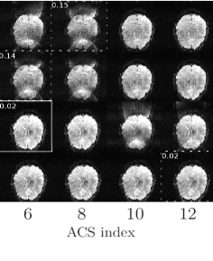
Figure 6: Images reconstructed from ACS data sets during which subject motion was introduced. Image rows 1 through 4 correspond to four different trials. During the acquisition of trials 1-3 the subject was instructed to move during ACS acquisition. During trial 4 the subject was instructed to remain motionless during the ACS acquisition. For brevity only the $10$ images associated with the even valued complete ACS data sets are shown rather than all $19$. For each trial the image corresponding to the highest or lowest value of the ACS perturbation metric $M_{s}$ is indicated by a dashed or solid bounding box respectively. The value of $M_{s}$ is given within the bounding box.

5 Discussion

In this work we demonstrated the effect of field inhomgeneity for one example situation to highlight the severity of artifacts that can result from $1$-shot ACS. (The mismatch phenomenon is treated in depth in A.) With increasing $R$, field inhomogeneity or EPI echo-spacing time the effects of main field inhomogeneity on $1$-shot ACS data acquisition are expected to become increasingly pronounced, suggesting a growing need for interleaved ACS data acquisition when acquiring ACS data for GRAPPA-accelerated EPI at 3T and above.

It is important to not substitute one source of error for another whenever possible. Therefore we have developed and demonstrated in this paper a means of acquiring segmented interleaved ACS data which greatly diminishes ACS motion contamination. Acquiring redundant ACS prior to an

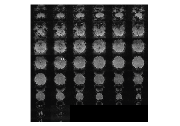
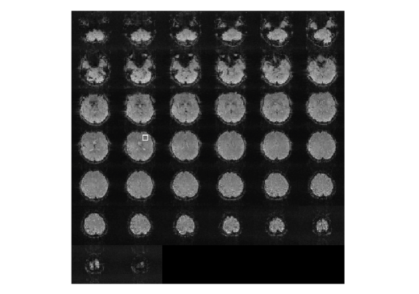
Figure 7: 2D multislice mosaics of tSNR images for the EPI time series. Top: Time series reconstructed by using the complete ACS data set with the largest valued perturbation metric. Bottom: Time series reconstructed by using the complete ACS data set with the smallest valued perturbation metric. Note that the same 100 volumes of accelerated ($R=2$) time series EPI data were used here, and only the ACS used to compute the synthesis coefficients differs between the two sets of images. For reference, the ratio of the mean tSNR, over the $5x5$ pixel region outlined in white, for smallest and largest valued $M_{s}$ is $tSNR_{smallest}/tSNR_{largest}=1.54$.

accelerated EPI time series allows the use of navigator echoes, conveniently already part of a product EPI pulse sequence, as a means of assessing motion corruption of GRAPPA ACS data. We have demonstrated that it is possible to retrieve the lowest motion-contaminated ACS data from a series of ACS data sets. Moreover we have demonstrated that motion during ACS has important consequences with respect to image artifact and time series tSNR. It is expected that this simple modification will greatly enhance the robustness of GRAPPA-accelerated EPI for fMRI, where subject motion during the initial part of the acquisition - the interleaved ACS - can render an entire time series worthless in a worst-case scenario, or with compromised tSNR as demonstrated in Figure 7.

In this work we acquired a fixed number of complete ACS data sets but the method could be further extended by looping on the ACS acquisition until the metric $M_{s}$ meets a prior criterion, thereby assuring that acceptable GRAPPA coefficients will be obtained in the presence of protracted motion during ACS acquisition. Figures 5 and 6 show that it should be possible to establish such a criterion for the metric $M_{s}$, although it would necessitate an automated way to advance the pulse program to the time series acquisition phase.

One limitation of the present method is a potential directional dependence of the navigator echoes. Since the navigators are projections of a 2D image slice (multiplied by a receive coil field) onto the frequency encoding axis, this method should be relatively insensitive to motion that is in the PE direction only. The nonuniformity of the receive coil field will introduce some sensitivity to motion that is in the PE direction only but if enhanced sensitivity to this type of motion is needed then a second navigator, spatially orthogonal to the first, could be used.

The work reported in this paper stands in contrast to the TGRAPPA EPI time series method investigated by Cheng (Cheng, 2010). In the TGRAPPA EPI times series method the effects of motion upon autocalibration are addressed by updating the synthesis coefficients at each point in the time series. In our work we take the perspective that a single calculation of the synthesis coeffcients will generate the greatest stability in the synthesis of the missing PE lines. We find support for this perspective in Cheng’s TGRAPPA work where he noted that in the absence of significant motion the use of frequently updated synthesis coefficients leads to a reduction of tSNR compared to the usual single calculation of synthesis coefficients. Indeed, in separate work, Cheng has shown recently (Cheng, 2012) that the temporal noise properties of GRAPPA EPI time series can be reduced via a single set of ACS for multiple time series acquisistions, rather than one ACS per acquisition. This increases still further the importance to acquire a motion-free ACS. Thus, the method presented here shows that it is possible to reduce the effects of motion during ACS acquisition while obtaining the desirable properties of the $R$-shot interleaved ACS, i.e. matched distortion characteristics for the ACS and the accelerated time series data. This should be of special interest in fMRI where motion is especially problematic.

From our perspective any motion during the time series and following the ACS leads to a spatial undersampling of the receive coil fields - the head may have moved into a region of the array from which no signal (or signal of low SNR) originated during the ACS. We see this spatial undersampling as a separate issue to be addressed in future work. It is a more involved problem than the simple method presented here that permits the acquisition of ACS uncontaminated by motion.

Appendix A GRAPPA and Field Inhomogeneity

We assume that there are $N_{c}$ receive coils in the receive array. For the reduced data set the signal from the nth receiver coil, after Fourier transform in the frequency-encoding $x$-direction and phase correction (Nyquist ghost correction) (Reeder et al., 1999), may be written as

$$s_{n}(x,mR)=\langle\rho,g_{nm}\rangle=\int\rho(x,y)g^{*}_{nm}(x,y)dy$$ (3)

where

$$g_{nm}(x,y)=g_{n}^{*}(x,y)e^{i2\pi mR\Delta ky}e^{-im\tau_{e}\phi(x,y)}=E^{m}g_{n}^{*}(x,y).$$ (4)

and where the definition of $E$ should be obvious, $g_{n}(x,y)$ is the receiver coil field (coil sensitivity), $R$ (an integer) is the reduction factor, $\phi(x,y)$ is the local field inhomogeneity offset of the main field, $\tau_{e}$ is the echo-spacing time and $m\in\mathbb{Z}$. Note that $\rho(x,y)$ is assumed to be an image that is compactly supported on $|y|,|x|<1/\Delta k$ and that the PE direction, $y$, will be the direction of acceleration. Also note that $s_{n}$, $g_{n}$ and $\phi$ will depend upon $z$ as well but we have omitted explicitly writing this dependence. Note that although $\langle\rho,g_{nm}\rangle$ is a function of $x$ we will suppress the $x$-dependence for the sake of an economy of symbols.

When the ACS data are acquired in $R$ interleaved segments the signal in the $n^{th}$ receiver coil will be

$$s^{R}_{n}(x,mR+p)=\langle\rho,g^{R}_{nm}\rangle=\int\rho(x,y)g^{R*}_{nm}(x,y)dy$$ (5)

where $p=0,\ldots,R-1$ and

$$g^{R}_{nm}(x,y)=g_{n}^{*}(x,y)e^{i2\pi(mR+p)\Delta ky}e^{-im\tau_{e}\phi(x,y)}=E^{m}E_{Ro}^{p}g_{n}^{*}(x,y).$$ (6)

The superscript $R$ denotes the R-shot trajectory for the complete ACS data set. When the complete ACS data set is acquired in one segment ($1$-shot trajectory) then the signal may be written as

$$s^{1}_{n}(x,mR+p)=\langle\rho,g^{1}_{nm}\rangle=\int\rho(x,y)g^{1*}_{nm}(x,y)dy$$ (7)

where

$$g^{1}_{nm}(x,y)=g_{n}^{*}(x,y)e^{i2\pi(mR+p)\Delta ky}e^{-i(mR+p)\tau_{e}\phi(x,y)}=E_{1}^{m}E_{1o}^{p}g_{n}^{*}(x,y).$$ (8)

and where the definition of the modulation operators $E_{R}$, $E_{Ro}$ $E_{1}$ and $E_{1o}$ should be obvious. The superscript $1$ denotes the $1$-shot trajectory for the complete ACS data set.

For a suitable $g_{n}(x,y)$ and $R$ the set $\{g_{nm}\}$, where $n=0,\ldots,N_{c}-1$ and $m\in\mathbb{Z}$, will form a frame (Christensen, 2003). Since $\{g_{nm}\}$ (reduction factor $R>1$) is assumed to be a frame we can write

$$\rho=\sum_{m^{\prime}=-\infty}^{\infty}\sum_{n^{\prime}=1}^{N_{c}}\langle\rho,g_{m^{\prime},n^{\prime}}\rangle S^{-1}g_{n^{\prime}m^{\prime}}$$ (9)

where $S$ is the frame operator for the frame $\{g_{nm}\}$ and where $\{S^{-1}g_{nm}\}$ is the canonical dual frame to the frame $\{g_{nm}\}$ (Christensen, 2003). Note that the dual frame depends upon $x$ although we will usually not indicate this explicitly. Note also that the canonical dual frame is only one of the possible and non-unique dual frames for which Equation (9) may be written. The canonical dual frame is a special dual frame in that it has the property that the $\langle\rho,S^{-1}g_{m^{\prime},n^{\prime}}\rangle$ have a minimal $l^{2}$-norm among all possible dual frames.

If the inverse frame operator could be found then equation (9) would form the fundamental means of obtaining $\rho$. In practice obtaining the inverse frame operator is mathematically difficult to obtain and this is at least partly due to the lack of an explicit knowledge of the coil sensitivities $g_{n}(x,y)$ (or the field inhomogeneity which may perturb the frame). Autocalibration methods provide an alternative to obtaining estimates of the dual frame and instead focus on determining the coefficients that transform one frame to another. We now take a closer look at the GRAPPA autocalibration method and how main-field inhomogeneity may affect the method.

Performing an analysis of $\rho$ given by equation (9) with respect to the frame $\{g^{R}_{nm}\}$ we obtain

$$\langle\rho,g^{R}_{nm}\rangle=\sum_{m^{\prime}=-\infty}^{\infty}\sum_{n^{\prime}=1}^{N_{c}}\langle\rho,g_{n^{\prime}m^{\prime}}\rangle\langle S^{-1}g_{n^{\prime}m^{\prime}},g^{R}_{nm}\rangle.$$ (10)

which we may write as

$$\langle\rho,g^{R}_{nm}\rangle=\sum_{m^{\prime}=-\infty}^{\infty}\sum_{n^{\prime}=1}^{N_{c}}\langle\rho,g_{n^{\prime}m^{\prime}}\rangle\langle S^{-1}E^{m^{\prime}}g_{n^{\prime}}^{*},E_{R}^{m}E_{Ro}^{p}g_{n}\rangle.$$ (11)

Since the frame operator $S$, and therefore its inverse, commutes with the modulation operator $E^{m}$ (Christensen, 2003) then equation (10) may be written as

$$\langle\rho,g^{R}_{nm}\rangle=\sum_{m^{\prime}=-\infty}^{\infty}\sum_{n^{\prime}=1}^{N_{c}}\langle\rho,g_{n^{\prime}m^{\prime}}\rangle\langle E^{m^{\prime}-m}S^{-1}g_{n^{\prime}}^{*},E_{Ro}^{p}g_{n}\rangle.$$ (12)

or according to equations (3) and (5)

$$s^{R}_{n}(x,mR+p)=\sum_{m^{\prime}=-\infty}^{\infty}\sum_{n^{\prime}=1}^{N_{c}}s_{n^{\prime}}(x,m^{\prime}R)\;c(m^{\prime}-m,n^{\prime},n,p,x)$$ (13)

where we have defined the synthesis coefficients

$$c(m^{\prime}-m,n^{\prime},n,p,x)=\langle E^{m^{\prime}-m}S^{-1}g_{n^{\prime}}^{*},E_{Ro}^{p}g_{n}\rangle$$ (14)

Notice that the $c$ depend upon the difference $m-m^{\prime}$ only. This particular dependence upon $m$ and $m^{\prime}$ allows us, through a change of indices and a truncation of the sum over $m^{\prime}$ (which must occur in a any practical setting), to write

$$s^{R}_{n}(x,mR+p)=\sum_{m^{\prime}=b_{1}}^{b_{2}}\sum_{n^{\prime}=1}^{N_{c}}s_{n^{\prime}}(x,mR+m^{\prime}R)\;c(m^{\prime},n^{\prime},n,p,x)$$ (15)

which is equivalent to the form of the GRAPPA equations given by Equation (1). The quantity $B=b_{2}-b_{1}$ is often referred to as the block size.

When the GRAPPA equations and the complete ACS data set are used to solve for the coefficients $c(m^{\prime},n^{\prime},n,p,x)$ it is usually the case that the number of unknown coefficients $c(m^{\prime},n^{\prime},n,p,x)$ exceeds the number of equations. When the number of ACS lines $N_{a}$ is an interger multiple of the reduction factor $R$ then there will be $N_{c}N_{a}(R-1)/R$ equations and $BN_{c}N_{a}/R$ unknown coefficients $c(m^{\prime},n^{\prime},n,p,x)$ at each point $x$. For a typical example of $N_{a}=24$, $N_{c}=12$ and $R=2$ the number of equations would be $144$ and the number of unknowns is $144B$. This presents a problem with respect to meeting necessary (but not sufficient) requirements for a unique solution set of the $c(m^{\prime},n^{\prime},n,p,x)$ - number of equations must be greater than or equal to the number of unknowns. To meet the necessary requirement it is usually assumed that the $c(m^{\prime},n^{\prime},n,p,x)$ vary little with respect to $x$ in the neighborhood of any $x$ in the FOV but that the signal does vary significantly with $x$. This allows one to use the ACS data at neighboring $x$ (at least $(d_{2}-d_{1})/(R-1)$ are needed) to locally determine the $c(m^{\prime},n^{\prime},n,p,x)$. Such an assumption implies that $g_{n}$, $S^{-1}$ and $\phi$ vary little about any $x$ in the FOV.

When the 1-shot trajectory is used to sample the complete ACS data set then, following steps similar to those given above, we can write

$$s^{1}_{n}(x,mR+p)=\sum_{m^{\prime}=-\infty}^{\infty}\sum_{n^{\prime}=1}^{N_{c}}s_{n^{\prime}}(x,m^{\prime}R)\langle E^{m^{\prime}}E_{1}^{-m}S^{-1}g_{n^{\prime}}^{*},E_{1o}^{p}g_{n}\rangle.$$ (16)

Since $E\neq E_{1}$ it is not possible to cast Equation (16) into the form of Equation (13) because the indices $m$ and $m^{\prime}$ do not appear as a difference only. Therefore, except when $\phi(x,y)=0$, it is necessary that the ACS data be collected over an R-shot trajectory in order for GRAPPA equations to strictly apply. As $R$ or $\phi(x,y)$ increases in magnitude the departure from the GRAPPA equations will increase. We can therefore expect the artifacts resulting from a 1-shot ACS calibration scan to increase with main field strength where susceptibility effects will be exacerbated and increasing reduction factors may be applied to combat the resulting distortions due to field inhomogeneity.

References

- Brau et al. (2008) Brau, A. C. S., Beatty, P. J., Skare, S., Bammer, R., 2008. Comparison of reconstruction accuracy and efficiency among autocalibrating data-driven parallel imaging methods. Magn. Reson. Med. 59, 382–395.
- Breuer et al. (2005) Breuer, F. A., Kellman, P., Griswold, M. A., Jakob, P. M., 2005. Dynamic autocalibrated parallel imaging using temporal grappa (tgrappa). Magn. Reson. Med. 53, 981–985.
- Cheng (2010) Cheng, H., 2010. On the application of tgrappa in functional mri. Proc. Intl. Soc. Mag. Reson. Med. 9, 169.
- Cheng (2012) Cheng, H., 2012. Variation of noise in multi-run functional mri using generalized autocalibrating partially parallel acquisition (grappa). J Magn Reson Imaging 35, 462–470.
- Christensen (2003) Christensen, O., 2003. An Introduction to Frames and Riesz Bases. Birkhauser, Boston, MA.
- Ehman and Felmlee (1989) Ehman, R. L., Felmlee, J. P., 1989. Adaptive technique for high-resolution mr imaging of moving structures. Radiology 173, 255–263.
- Griswold et al. (2002) Griswold, M. A., Jakob, P. M., Heidemann, R. M., Nittka, M., Jellus, V., Wang, J., Kiefer, B., Haase1, A., 2002. Generalized autocalibrating partially parallel acquisitions (grappa). Magn. Reson. Med. 47, 1202–1210.
- Heidemann et al. (2010) Heidemann, R. M., Porter, D. A., Anwander, A., Feiweier, T., Heberlein, K., Knosche, T. R., Turner, R., 2010. Diffusion imaging in humans at 7t using readout-segmented epi and grappa. Magn. Reson. Med. 64, 9–14.
- Holdsworth et al. (2009) Holdsworth, S. J., Skare, S., Newbould, R. D., Bammer, R., 2009. Robust grappa-accelerated diffusion-weighted readout-segmented (rs)-epi. Magn. Reson. Med. 62, 1629–1640.
- Hu and Kim (1994) Hu, X., Kim, S. G., 1994. Reduction of signal fluctuation in functional mri using navigator echoes. Magn Reson Med 31, 495–503.
- Jakob et al. (1998) Jakob, P. M., Griswold, M. A., Edelman, R. R., Sodickson, D. K., 1998. Auto-smash: A self-calibrating technique for smash imaging. MAGMA 7, 42–54.
- Kellman et al. (2001) Kellman, P., Epstein, F. H., McVeigh, E. R., 2001. Adaptive sensitivity encoding incorporating temporal filtering (tsense). Magn Reson Med 45, 846–852.
- Kim et al. (1996) Kim, S. G., Hu, X., Adriany, G., Ugurbil, K., 1996. Fast interleaved echo-planar imaging with navigator: High resolution anatomic and functional images at 4 tesla. Magn Reson Med 35, 895–902.
- Larsson et al. (2003) Larsson, E. G., Erdogmus, D., Yan, R., Principe, J. C., Fitzsimmons, J. R., 2003. Snr-optimality of sum-of-squares reconstruction for phased-array magnetic resonance imaging. J. Mag. Reson. 163, 121–123.
- Law et al. (2008) Law, C. S., Liu, C., Glover, G. H., 2008. Sliding-window sensitivity encoding (sense) calibration for reducing noise in functional mri (fmri). Magn. Reson. Med. 60, 1090–1103.
- Nguyen et al. (1998) Nguyen, Q., Clemence, M., Ordidge, R. J., 1998. Clemence m, ordidge rj. the use of intelligent re-acquisition to reduce scan time in mri degraded by motion. Proc. ISMRM 6th Annual Meeting, 134.
- Porter and Heidemann (2009) Porter, D. A., Heidemann, R. M., 2009. High resolution diffusion-weighted imaging using readout-segmented echo-planar imaging, parallel imaging and a two-dimensional navigator-based reacquisition. Magn. Reson. Med. 62, 468–475.
- Pruessmann et al. (1999) Pruessmann, K. P., Weiger, M., Scheidegger, M. B., Boesiger, P., 1999. Sense: Sensitivity encoding for fast mri. Magn. Reson. Med. 42, 952–962.
- Reeder et al. (1999) Reeder, S. B., Faranesh, A. Z., Atalar, E., McVeigh, E. R., 1999. A novel object-independent ”balanced” reference scan for echo-planar imaging. J Magn Reson Imaging 9, 847 – 852.
- Roemer et al. (1990) Roemer, P. B., Edelstein, A., Hayes, E., Souza, P., Muellera, . M., Harris, R. L., 1990. The nmr phased array. Magn. Reson. Med. 16, 192–225.
- Schmiedeskamp et al. (2010) Schmiedeskamp, H., Newbould, R. D., Pisani, L. J., Skare, S., Glover, G. H., Pruessmann, K. P., Bammer, R., 2010. Improvements in parallel imaging accelerated functional mri using multiecho echo-planar imaging. Magn. Reson. Med. 63, 959–969.
- Sodickson and Manning (1997) Sodickson, D. K., Manning, W. J., 1997. Simultaneous acquisition of spatial harmonics (smash): Fast imaging with radiofrequency coil arrays. Magn. Reson. Med. 38, 591–603.