Wetting Transition in the Two-Dimensional Blume-Capel Model: A Monte Carlo study

Abstract

The wetting transition of the Blume-Capel model is studied by a finite-size scaling analysis of $L\times M$ lattices where competing boundary fields $\pm H_{1}$ act on the first row or last row of the $L$ rows in the strip, respectively. We show that using the appropriate anisotropic version of finite size scaling, critical wetting in $d=2$ is equivalent to a “bulk” critical phenomenon with exponents $\alpha=-1$, $\beta=0$, and $\gamma=3$. These concepts are also verified for the Ising model. For the Blume-Capel model it is found that the field strength $H_{1c}(T)$ where critical wetting occurs goes to zero when the bulk second-order transition is approached, while $H_{1c}(T)$ stays nonzero in the region where in the bulk a first-order transition from the ordered phase, with nonzero spontaneous magnetization, to the disordered phase occurs. Interfaces between coexisting phases then show interfacial enrichment of a layer of the disordered phase which exhibits in the second order case a finite thickness only. A tentative discussion of the scaling behavior of the wetting phase diagram near the tricritical point also is given.

PACS: 68.08.Bc, 68.35.Rh, 64.60F-, 05.70.Fh

I Introduction

Understanding interfacial phenomena at boundaries 1 ; 2 ; 3 ; 4 such as free surfaces of solids, or walls confining fluids, etc., is a topic of very high interest in current condensed matter research, driven by important applications, e.g. in micro- or nanofluidics, design of smart nanomaterials 5 ; 6 ; 7 ; 8 , etc. But it is also of fundamental interest as a problem of statistical mechanics. It is only the latter aspect that will be in our focus here, and hence we shall not deal here with wetting properties 9 ; 10 ; 11 ; 12 ; 13 ; 14 ; 15 ; 16 ; 17 of specific materials, but rather consider wetting in the framework of a simple lattice model with nearest neighbor interactions and short-range forces due to the walls.

In this spirit, a large amount of work has been devoted to the study of simple Ising models with boundary fields; see e.g. 18 for a review, and 19 ; 20 ; 21 ; 22 ; 23 ; 24 ; 25 ; 26 ; 27 ; 28 ; 29 ; 30 ; 31 ; 32 ; 33 ; 34 ; 35 ; 36 ; 37 ; 38 ; 39 ; 40 for some pertinent original work. Spin reversal symmetry of this generic model implies that phase coexistence between the ordered phases with positive and negative spontaneous magnetization occurs at zero bulk field (H=0) in the thermodynamic limit in the bulk; the same holds still true when one considers a thin film of a finite thickness $L$ with surfaces at which boundary fields $H_{1}$, $H_{L}$ act, provided one considers the antisymmetric situation $H_{1}=-H_{L}$, avoiding “capillary condensation” 18 ; 20 ; 22 , i.e. a shift of bulk coexistence to nonzero value of the bulk field due to boundary effects. The latter phenomena is interesting in its own right, e.g. 41 , and can also be studied in Ising models choosing boundary fields $H_{1}=H_{L}$, e.g. 42 ; 43 ; 44 , but this problem will not be followed up here.

In principle, the study of a wetting transition, where the boundary induces the formation of a macroscopically thick film of the phase that it prefers, coexisting with the other phase separated by an interface at a macroscopic distance from the boundary, requires to consider the limit $L\rightarrow\infty$. For any finite $L$ in the antisymmetric thin film geometry, or thin strip geometry, when one considers $d=2$ dimensions rather than $d=3$, one does not find a wetting transition, but rather the ”interface localization-delocalization transition” 18 ; 27 ; 28 ; 29 ; 30 ; 31 ; 32 ; 33 ; 37 ; 38 ; 39 : for temperatures above $T_{c}(L,H_{1})$ but below the transition temperature $T_{cb}$ of the bulk Ising model, the interface between the coexisting phases is “delocalized”, freely fluctuating in the center of the film (or strip, respectively). Here, by center we mean the plane (or line) ($L+1)/2$, if we label the layers (rows) of the Ising lattice parallel to the boundaries from $n=1$ to $n=L$. However, for $T<T_{c}(L,H_{1})$ the interface is tightly bound, and hence “localized”, near one of the two boundaries. One predicts, however, that for large $L$ the transition temperature $T_{c}(L,H_{1})$ converges rapidly to the wetting transition temperature $T_{w}(H_{1})$ of the semi-infinite system 29 ; 30 , and this prediction is consistent with the numerical simulations 27 ; 28 ; 31 ; 32 ; 33 ; 38 ; 39 .

One aspect of wetting in the Ising model that found great attention is the behavior near bulk criticality. One can show that for a second-order wetting transition the inverse function $H_{1c}(T)$ of $T_{w}(H_{1})$ behaves as 21

$$H_{1c}(T)\propto(T_{cb}-T)^{\Delta_{1}}\quad,$$ (1)

where $\Delta_{1}$ is the critical exponent that controls the scaling behavior with the surface field $H_{1}$ near bulk criticality 45 ; 46 ; 47 . While $\Delta_{1}$ in $d=3$ is only known approximately from numerical work, in $d=2$ Abraham’s exact solution for the Ising model 19 implies $\Delta_{1}=\frac{1}{2}$. Note that on the square lattice with exchange constant $J$ between nearest neighbors the wetting transition occurs for $H_{1c}$ given as the solution of

$$\exp(2J/k_{B}T)[\cosh(2J/k_{B}T)-\cosh(2H_{1c}/k_{B}T)]$$

$$=\sinh(2J/k_{B}T)\quad,$$ (2)

and the bulk critical point occurs at $\exp(2J/k_{B}T_{cb})=\sqrt{2}+1$ 48 .

An intriguing question is, of course, to study how the wetting behavior gets modified if the bulk phase transition changes its character. E.g., a simple extension of the Ising model is the Blume-Capel model 49 ; 50 , where each lattice site (i) can be in one of three states $S_{i}=+1$, $S_{i}=0$, $S_{i}=-1$ and the Hamiltonian becomes

$$\mathcal{H}=-J\sum\limits_{\langle i,j\rangle}S_{i}S_{j}+D\sum\limits_{i}S_{i}^{2}\quad,$$ (3)

where the “crystal field” $D$ controls the density of “vacancies”, i.e. sites with $S_{i}=0$.

When $D\rightarrow-\infty$ vacancies are excluded, and the model reduces to the standard two state Ising model, but when $D/J$ is of order unity, one has a nontrivial bulk phase diagram with a tricritical point 51 at $D=D_{t}$. For the square lattice, this tricritical point occurs at $D_{t}/J\tilde{=}1.965(5)$ and $k_{B}T_{t}/J\tilde{=}0.609$ (5). For $D>D_{t}$ the transition at $T_{c}(D)$ is first order: two phases with opposite nonzero magnetization and the disordered phase (with zero magnetization) coexist.

From the universality principle, we expect that Eq. (1) with $\Delta_{1}=\frac{1}{2}$ would also hold in the second-order region of the Blume-Capel model for $D<D_{t}$, but to our knowledge this assumption has not yet been tested. Providing evidence for this assumption is one of the goals of the present paper. Right at the tricritical point, however, the behavior should be different: instead of Eq. (1) we now expect

$$H_{1c}(D_{t},T)\propto(T_{t}-T)^{\Delta_{1t}}\quad,$$ (4)

where the exponent $\Delta_{1t}$ in $d=3$ is expected to be $\Delta_{1t}=1/4$ 52 , the prediction due to Landau mean-field theory, which is expected to hold in $d=3$, apart from logarithmic corrections 51 . While in $d=2$ the tricritical exponents in the bulk are not those of mean-field theory 51 , for the Ising model universality class to which the tricritial point of the Blume-Capel model belongs 51 , they are exactly known from conformal invariance 53 ; 54 ; 55 . E.g. in standard notation of critical exponents 56 ; 57 ) $\alpha_{t}=8/9$, $\beta_{t}=1/24$, $\gamma_{t}=37/36$, $\nu_{t}=5/9$, etc. To our knowledge, $\Delta_{1t}$ for this problem is not yet known, however.

When one considers the wetting transition for the part of the transition line $T_{cb}(D)$ that is first order $(D>D_{t})$, the wetting transition $H_{1c}(T)$ ends at this line at a nonzero value of the surface field,

$$H^{*}_{1c}(D)=H_{1c}(D,T=T_{cb}(D))\quad.$$ (5)

We expect that another power law will exist when $D$ approaches $D_{t}$ from below,

$$H^{*}_{1c}(D)\propto(D-D_{t})^{\zeta}\quad,$$ (6)

but again we are not aware of predictions relating to this critical exponent $\zeta$. The evaluation of $\zeta$ from numerical work is a very challenging task, because it requires to locate both the tricritical point and the wetting transitions with very high accuracy.

Finally, a very interesting aspect relates to the character of the interface between the coexisting phases with positive and negative magnetization, when one approaches the bulk phase transition: then interfacial adsorption of the third phase (the disordered phase) at the interface can occur 58 ; 59 ; 60 . If we denote the coexisting bulk phases as $A$ and $B$, approaching the bulk transition line in the second-order region one expects an interfacial wetting transition $A|B\rightarrow A|DO|B$, where $DO$ stands symbolically for an intruding layer of the disordered phase having predominantly states where $S_{i}=0$ dominates at the interface. To quantify this effect one considers the net adsorption defined by

$$W_{o}(T)=N^{-1}\sum\limits_{i=1}^{M}[\langle\delta_{0,S_{i}}\rangle_{1|-1}-\langle\delta_{0,S_{i}}\rangle_{1|1}]\quad,$$ (7)

where $N$ is the total number of lattice sites, $M$ is the number of lattice sites per row parallel to the walls, $\delta_{\alpha,\beta}$ is the Kronecker symbol, and $\langle\cdots\rangle_{1|-1}$ a statistical average in the presence of an interface ($A=1$, $B=-1$), while $\langle\cdots\rangle_{1|1}$ is the corresponding average for an equivalent system but without interfaces. Since $\delta_{0,S_{i}}=1-S_{i}^{2}$, one can conclude also that $W_{0}(T)=(\partial\sigma_{AB}/\partial D)$ where $\sigma_{AB}$ is the interfacial tension for the considered interface. Since for $D<D_{t}$ the bulk phase transition of the Blume-Capel model falls in the Ising universality class, we know that $\sigma_{AB}\propto(1-T/T_{cb}(D))^{\mu}$ with $\mu=(d-1)\nu=1$ for the Blume-Capel model. Writing $t=1-T/T_{cb}(D)$, we find

$$W_{0}(T)=\Big{(}\frac{\partial\sigma_{AB}}{\partial t}\Big{)}\Big{(}\frac{\partial t}{\partial D}\Big{)}\propto t^{\mu-1}={\rm const}\quad;$$ (8)

thus if we define a divergence of interfacial adsorption via

$$W_{0}(T)\propto t^{-\omega}\quad,$$ (9)

we find $\omega=0$ for $D<D_{t}$, i.e. in the Ising-like regime there should be no critical divergence of the net adsorption. However, right at the tricritical point, the behavior should be different: from $\nu=5/9$ as quoted above we conclude $W_{0}(T)\propto t^{-\omega}$ with $\omega=4/9$ for $D=D_{t}$. This result is consistent with Monte Carlo results of Selke et al. 59 .

For $D_{t}=1.965<D\leq 2$ the transition of the Blume-Capel model is believed to be first order, and the emerging interfaces $A|DO$ and $DO|B$ remain sharp as $T\rightarrow T_{c}(D)$. Reducing the problem to interfaces in the solid-on-solid model, one can argue that Eq. (9) also holds in the first-order region, but $\omega=1/3$ 12 . These considersations have been checked by early Monte Carlo work 58 ; 59 ; 60 for interfaces between coexisting bulk phases, but no study in the context of wetting at external boundaries has as yet been performed, to our knowledge.

In the present work, we wish to contribute filling this gap and study wetting behavior for the two-dimensional Blume-Capel model in the case of thin films for which surface fields at the boundaries act, as described in Sec. 2. However, in order to do so, we have found it necessary to reconsider the simulation methodology for the study of critical wetting. In fact, by applying Monte Carlo simulations, we shall necessarily study finite systems, namely strips of width $L$ (in $y$-direction) and length $M$ (in $x$-direction, where a periodic boundary condition acts). As a consequence, finite size effects matter, and hence in the next section we also shall give the background on the proper finite size scaling analysis of such simulation “data”, for the case of critical wetting in $d=2$ dimensions, taking into account that one deals there with an anisotropic critical phenomenon of a special character: if we consider the magnetization $m$ of the strip as the “order parameter” of the transition, its critical exponent $\beta=0$. This fact does not seem to have found much attention in the previous Monte Carlo studies of critical wetting in $d=2$ 28 ; 38 . This revised methodology for the study of critical wetting, which is outlined in Sec. 2, is another important result of our work.

Sec. 3 then presents our Monte Carlo results, which then are analyzed according to these concepts, and the wetting transitions are discussed for a variety of choices of $D$, both cases $D<D_{t}$, $D=D_{t}$ and $D>D_{t}$ will be considered. Sec. 4 then discusses our result on interfacial adsorption, and Sec. 5 summarizes our conclusions.

II THEORETICAL BACKGROUND AND DETAILS ON SIMULATION METHODS

II.1 The model

We consider the Hamiltonian of the $3$-state Blume-Capel model 49 ; 50 where each lattice site $i$ carries a spin $S_{i}$ that can take on the values $S_{i}=\pm 1,0,$ at a square lattice in a $L\times M$ geometry, where periodic boundary conditions act in the $x$-direction (where the lattice is $M$ rows long), while free boundary conditions are used in the $y$-direction, where boundary fields $H_{1}$, $H_{L}$ act on the first and the last row. Thus the Hamiltonian is

$$\mathcal{H}=-J\sum\limits_{\langle i,j\rangle}S_{i}S_{j}+D\sum\limits_{i}S^{2}_{i}$$ (10)

$$-H\sum\limits_{i}S_{i}-H_{1}\sum\limits_{i\in\,{\rm row}1}S_{i}-H_{L}\sum\limits_{i\in\,{\rm row}L}S_{i}\quad.$$

Here $J$ is the exchange constant between spins at nearest neighbor sites, which we take homogeneous throughout the system. Thus, we disregard the possibility to take the exchange $J_{s}$ in the boundary rows different from the exchange $J$ in the interior of the system, that is frequently considered in studies of wetting phenomena in the Ising model 18 ; 25 ; 26 ; 31 ; 32 ; 33 ; 39 . The bulk field $H$ acts on all lattice sites, while the “surface fields” 45 ; 46 ; 47 only act on the spins in the first (1) and last (L) row, where the free boundary conditions apply.

We also specialize on the particular antisymmetric situation $H_{1}=-H_{L}<0$ and consider the thermodynamic limit $(L\rightarrow\infty$, $M\rightarrow\infty$) before we consider the limit $H\rightarrow 0^{+}$. Then, the system undergoes two phase transitions: at the temperature $T_{cb}(D)$ the phase transition occurs from the disordered “paramagnetic” phase to the ordered “ferromagnetic” phase, where we have used the terminology of the Ising model. Taking the lattice spacing as our unit of length, the total number of spins is just the product of the linear dimensions of the system, $N=LM$. In fact, when we define the magnetization $m$ per lattice site as

$$m=\frac{1}{N}\sum\limits_{i=1}^{N}S_{i}\quad,$$ (11)

its thermal expectation value $\langle m\rangle_{T}$ for temperatures $T<T_{cb}(D)$ will be nonzero and positive in the considered limit. However, a second phase transition occurs at a lower temperature $T_{w}(H_{1})$ for small enough absolute values $|H_{1}|$ of the surface field: Note that the surface field $H_{1}$ is oppositely oriented to the positive bulk field $H$, but $H\rightarrow 0^{+}$ while $H_{1}$, stays finite. Thus, near $T_{cb}(D)$ the surface field stabilizes a macroscopically thick layer of negative magnetization near the lower boundary, where $H_{1}<0$ acts, separated by an interface from the bulk, where the magnetization is positive. At $T_{w}(H_{1})$, a transition occurs where this interface gets localized near the lower boundary: in the extreme case, the domain with negative magnetization disappears completely. In the Ising model, which results from Eq. (10) as the limiting case $D\rightarrow-\infty$, this wetting transition is second order throughout the regime $0<|H_{1}|<J$.

II.2 Critical wetting in $d=2$ dimensions: A brief review

For the semi-infinite system described above, the wetting transition is a singularity of the surface excess free energy $f_{s}^{(1)}(T;H,H_{1})$, defined from standard decomposition of the total free energy into the bulk term and boundary terms, for $L\rightarrow\infty$, $M\rightarrow\infty$

$$F(T,H,H_{1},H_{L},L,M)/(LM)=f_{b}(T,H)+\frac{1}{L}f_{s}^{(1)}(T,H,H_{1})$$

$$\hskip 136.5733pt+\frac{1}{L}f_{s}^{(L)}(T,H,H_{L})\quad.$$ (12)

The singular part of this boundary free energy, also called “wall tension” or “wall excess free energy” 1 ; 2 ; 9 ; 10 ; 11 ; 12 ; 13 ; 14 ; 18 , near $T_{w}(H_{1})$ is expected to satisfy a scaling behavior 12 ; 21 ; 57 ; 61 ; 62 where $t=1-T/T_{w}(H_{1})\rightarrow 0$,

$$f_{s,{\rm sing}}^{(1)}/k_{B}T=|t|^{2-\alpha_{s}}\tilde{F}_{s}(H|t|^{-\Delta_{s}})\quad.$$ (13)

$\tilde{F}_{s}$ being a scaling function that we do not specify here. This is analogous to standard scaling in the bulk near $T_{cb}$ 56 , where $\tau=1-T/T_{cb}\rightarrow 0$,

$$f_{b,{\rm sing}}/k_{B}T=|\tau|^{2-\alpha}\tilde{F}_{b}(H|\tau|^{-\Delta})\quad.$$ (14)

In Eq. (14), $\alpha$ is the specific heat exponent, and the “gap exponent” $\Delta$ is related to the standard exponents $\beta$ of the spontaneous magnetization $(\langle m\rangle_{T}\propto\tau^{\beta})$ and $\gamma$ of the susceptibility $(\chi=(\partial\langle m\rangle/\partial H)_{T})\propto|\tau|^{-\gamma}$ via the scaling relation $\Delta=\gamma+\beta$ 56 . Thus $\alpha_{s}$, $\Delta_{s}$ are analogous exponents characterizing the singular behavior of the critical wetting transition in $d=2$ dimensions.

As always when one considers a critical phenomenon, a diverging correlation length exists. Since wetting can be viewed as an “interface unbinding” transition 9 ; 10 ; 11 ; 12 ; 13 ; 14 ; 15 ; 16 ; 17 ; 18 when approached from below, it is natural to study the correlation function $C(x)$ describing the correlation of fluctuations of the height of the contour $\ell(x)$ separating the domain with negative magnetization near the lower boundary from the region with positive magnetization in the bulk. Defining $\delta\ell(x)$ as $\delta\ell(x)=\ell(x)-\langle\ell\rangle$, this yields

$$G(x)=\langle\delta\ell(0)\delta\ell(x)\rangle_{T}\quad,$$ (15)

noting translational invariance in $x$-direction. By $\langle...\rangle_{T}$ we denote an average in the canonical ensemble at temperature $T$; in the following the subscript $T$ will be omitted. Near critical wetting in $d=2$ $G(x)$ takes the scaling form 61

$$G(x)=x^{-(1+\eta_{||})}g(x/\xi_{||})\quad,$$ (16)

writing analogously to the decay of bulk correlations near criticality, $G(r)=r^{-(d-2+\eta)}g(r/\xi_{b})$, with $\eta$, $\eta_{||}$ being appropriate exponents describing the variation of these correlations at large distances right at bulk criticality or critical wetting, where $\xi_{b}$ (or $\xi_{||})$ is infinite. For $\xi_{||}$, a scaling relation analogous to Eq. (13) holds,

$$\xi_{||}=t^{-\nu_{||}}\tilde{\xi}_{||}(Ht^{-\Delta_{s}})\quad;$$ (17)

again this Ansatz is inspired by the corresponding bulk behavior,

$$\xi_{b}=\tau^{-\nu}\tilde{\xi}_{b}(H|\tau|^{-\Delta})\quad,$$ (18)

and again $\tilde{\xi}_{||}$, $\tilde{\xi}_{b}$ are scaling functions that we do not specify here.

We disregard here the problem that in general a nonlocal theory 63 ; 64 ; 65 ; 66 is required 40 , since it does not change the following conclusions. Capillary wave theory implies that $\eta_{||}=0$, so there is no second independent critical exponent as in the bulk. For a more detailed reasoning to explain why for the case of critical wetting with short-range forces the exponent $\eta_{||}$ is zero in all dimensions, and hence there is a single independent critical exponent, we refer to the literature 12 . Remember that using hyperscaling relations $d\nu=2-\alpha=\gamma+2\beta$ and the scaling law $\gamma=\nu(2-\eta)$ one can express all static critical exponents just in terms of only two independent exponents $\nu$ and $\eta$ in the bulk 56 . For critical wetting, in $d=2$, there is only one independent critical exponent namely, 11

$$\nu_{||}=2$$ (19)

and the hyperscaling relation for interfacial phenomena in $d=2$ dimensions $\nu_{||}=2-\alpha_{s}$ 12 then implies $\alpha_{s}=0$. From Eq. (16) we then conclude that on a length scale $x$ the interface exhibits (at $t=0$) a mean-square displacement also proportional to $x$, while for $t>0$ one concludes that on the length scale $\xi_{||}$ the mean-square displacement in $y$-direction also is proportional to $\xi_{||}$, while for $x\gg\xi_{||}$ the correlation $G(x)\rightarrow 0$. This leads to the conclusion that the correlation length $\xi_{\bot}$ describing the fluctuations of the interface in $y$ direction scales as

$$\xi^{2}_{\bot}\propto\xi_{||}\quad,\quad$$

$$\xi_{\bot}\propto t^{-\nu_{\bot}}({\rm for}\,H=0),\nu_{\bot}=1\quad.$$ (20)

Noting from Eq. (13) that surface excess magnetization $m_{s}$ and surface excess susceptibility $\chi_{s}$ follow from derivatives with respect to the field

$$m_{s}=-\partial f_{s}^{(1)}(T,H,H_{1})/\partial H|_{T,H_{1}}\quad,$$ (21)

$$\chi_{s}=-(\partial^{2}f_{s}^{(1)}(T,H,H_{1})/\partial H^{2})_{T,H_{1}}$$ (22)

we conclude that these quantities have the singularities

$$m_{s}\propto t^{2-\alpha_{s}-\Delta_{s}}\quad,\quad m_{s}\propto t^{\beta_{s}}\quad,$$ (23)

and

$$\chi_{s}\propto t^{2-\alpha_{s}-2\Delta_{s}}\quad\cdot\quad\chi_{s}\propto t^{-\gamma_{s}}\quad.$$ (24)

Using then the consideration that this excess susceptibility is just caused by displacements of the interface between the domain of negative magnetization at the boundary and the bulk, one can use Eq. (16) to deduce a further scaling relation between $\Delta_{s},$ $\nu_{||}$ and $\eta_{||}$, namely 12

$$\Delta_{s}=(\nu_{||}/2)[(d-1)+2-\eta_{||}]=3,\quad(d=2)\quad.$$ (25)

Also the excess magnetization $m_{s}$ obviously simply is related to $\langle\ell\rangle$, and we have, in $d=2$,

$$m_{s}\propto\langle\ell\rangle\propto t^{-1}\propto\xi_{\bot}\quad.$$ (26)

Thus, near to critical wetting in $d=2$ the typical mean distance of the interface from the wall and the typical excursions of this interface from its mean are of the same order, $\nu_{\bot}=-\beta_{s}=1$.

II.3 Finite-size scaling: wetting vs bulk transitions

All above relations did refer to the case that we were considering the limits $M\rightarrow\infty$ and $L\rightarrow\infty$ first, and then consider the limits $H\rightarrow 0$, $t\rightarrow 0$ near the wetting transition. While such an approach is natural in the context of analytic theories 10 ; 11 ; 12 , it it not sufficient to understand simulations, where we wish to take these limits in reverse order. When $L$ is kept large but finite, it is clear that for temperatures above the wetting transition and $H=0$ there is no physical distinction between the domain with negative magnetization in the lower half of the system and the domain with positive magnetization in the upper half: Previously, for the semi-infinite case, the positive magnetization in the bulk was singled out by taking the limit $H\rightarrow 0^{+}$ first, and then the positive boundary field $H_{L}$ for $L\rightarrow\infty$ was irrelevant, while for $L$ finite it is critical to maintain the symmetry of the situation with respect to the sign of the magnetization for $H=0$. As a consequence, we conclude that for the present situation there is no bulk magnetization to consider, and it rather is the total magnetization of the system or strictly speaking, its absolute value, which undergoes a transition from zero to a nonzero value when we cross the wetting transition temperature, and extrapolate simulation results towards $L\rightarrow\infty$.

As a consequence of this consideration, we propose a scaling assumption for the distribution function $P_{L,M}(m)$ of the total magnetization in this finite geometry as follows 67 ; 68

$$P_{L,M}(m)=\xi_{||}^{\beta/\nu_{||}}\tilde{P}(L^{\nu_{||}/\nu_{\bot}}/M,M/\xi_{||},m\xi_{||}^{\beta/\nu_{||}})\quad.$$ (27)

Note that this expression generalizes the standard expression for finite-size scaling in isotropic systems that have linear dimension $L$ in all spatial directions 69 , as appropriate for phase transitions in the bulk

$$P_{L}(m)=\xi_{b}^{\beta/\nu}\tilde{P}_{b}(L/\xi_{b},m\xi^{\beta/\nu}_{b})$$ (28)

to systems with anisotropic linear dimensions $L,M$ and anisotropic correlation length exponents $\nu_{||}$, $\nu_{\bot}$. While for isotropic critical phenomena an anisotropic system shape would lead to a dependence simply on the “aspect ratio” $L/M$ of the system, the fact that $M$ scales with $\xi_{||}$ and $L$ scales with $\xi_{\bot}$ can be used to demonstrate 67 ; 68 that the $L$-dependence enters via “the generalized aspect ratio” $L^{\nu_{||}/\nu_{T}}/M$ in the scaling function, Eq. (27). With $\nu_{||}=2$, $\nu_{\bot}=1$ we simply have an argument $L^{2}/M$, which needs to be kept constant when the variation with $M$ is studied. Such generalizations of finite-size scaling to anisotropic criticality have been discussed earlier for the Kasteleyn transition X ; XI , which also exhibits $\nu_{||}=2\nu_{\bot}$ and hence the same generalized aspect ratio $L^{2}/M$ applies. The prefactor $\xi_{||}^{\beta/\nu_{||}}$ in Eq. (27), and likewise the prefactor $\xi^{\beta/\nu}_{b}$ in Eq. (28), ensures that the probability $P_{L,M}(m)$ can be properly normalized,

$$\int\limits_{-1}^{+1}P_{L,M}(m)dm=1\quad.$$ (29)

Taking now suitable moments of $P_{L,M}(m)$, analogous to the procedure at isotropic phase transitions in the bulk 69 ; 70 , we obtain

$$\langle|m|\rangle=\int\limits_{-1}^{+1}dm|m|P_{L,M}(m)=$$

$$=\xi_{||}^{-\beta/\nu_{||}}\tilde{m}(L^{\nu_{||}/\nu_{\bot}}/M,M/\xi_{||})\quad,$$ (30)

$$\langle m^{2k}\rangle=\xi_{||}^{-2k\beta/\nu_{||}}\tilde{m}_{2k}(L^{\nu_{||}/\nu_{\bot}}/M,M/\xi_{||}),\quad$$

$$k=1,2,\cdots\quad.$$ (31)

In particular, from Eqs. (II.3), (II.3) we derive the standard behavior for the “susceptibility”. We denote it by $\chi^{\prime}$ since $\langle|m|\rangle^{2}$ rather than $\langle m\rangle^{2}$ is subtracted, see Ref. 70 for a discussion. So, one has

$$k_{B}T\chi^{\prime}=LM(\langle m^{2}\rangle-\langle|m|\rangle^{2})\quad,$$ (32)

and hence

$$k_{B}T\chi^{\prime}=LM\xi_{||}^{-2\beta/\nu_{||}}\tilde{\chi}(L^{\nu_{||}/\nu_{\bot}}/M,M/\xi_{||})\quad,$$ (33)

with the scaling function $\tilde{\chi}\equiv\tilde{m}_{2}-(\tilde{m})^{2}$, omitting all arguments for simplicity.

Now the key task is to identify the “order parameter exponent” $\beta$ in the context of this description of a critical wetting transition. For this purpose, we note that the singular behavior of $\chi^{\prime}$ can only be due to the singular behavior of $\chi_{s}\propto t^{-4}$, Eq. (24), where we used the results $\alpha_{s}=0$, $\Delta=3$. A key point to note is that $\chi^{\prime}$ was normalitzed per spin, relating to the total volume $LM$, while $\chi_{s}$ in Eq. (24) is taken relative to boundary sites, so is only normalized by $M$. Hence we conclude that at $T_{w}$, we have, using $L^{2}/M=c$ in Eq. (33) to eliminate $L$

$$k_{B}T\chi^{\prime}\propto\sqrt{c}M^{3/2-2\beta/\nu_{||}}$$ (34)

irrespective of how the finite constant $c$ is chosen. Writing then

$$k_{B}T\chi^{\prime}|_{T_{w}}=k_{B}T\chi_{s}/L=k_{B}T\chi_{s}M^{-1/2}c^{-1/2}$$ (35)

and using a finite-size scaling relation for $\chi_{s}$

$$\chi_{s}=t^{-4}\tilde{\chi}(M/\xi_{||})\propto\xi^{2}_{||}\tilde{\chi}(M/\xi_{||})\propto M^{2}\quad,T=T_{w}$$ (36)

and hence we find

$$k_{B}T\chi^{\prime}|_{T_{w}}\propto M^{3/2}(\propto L^{3})\quad.$$ (37)

Comparison of Eqs. (34) and (37) yields a central result of this section, namely

$$\beta=0\quad,$$ (38)

and Eq. (37) also can be interpreted in terms of the standard finite-size scaling result

$$k_{B}T\chi^{\prime}|_{T_{w}}\propto M^{\gamma/\nu_{||}}\quad,\quad\gamma=3\quad.$$ (39)

Second order transitions with an exponent $\beta=0$ are rather unusual; for another recent example see Jaubert et al. XII . In the present case, we can also understand it from the fact that $\langle|m|\rangle$ must tend to $m_{b}$ in the thermodynamic limit in the partially wet phase, where the interface is bound to one of the walls up to the transition point, while in the wet phase for the considered limit $\langle|m|\rangle=0$. It is interesting to note that these critical exponents also satisfy the usual scaling relation with the gap exponent $\Delta_{s}$ introduced in Eq. (13),

$$\gamma+\beta=\Delta_{s}=3\quad,$$ (40)

as well as the hyperscaling relation for anisotropic bulk critical phenomena in $d=2$ dimensions,

$$\nu_{||}+\nu_{\bot}=2\beta+\gamma=3\quad.$$ (41)

One should not confuse the exponent $\beta$ of the total magnetization, resulting in the limit $L\rightarrow\infty$, $M\rightarrow\infty$, $L^{2}/M=c$, with the exponent $\beta_{s}$ of the surface excess magnetization $m_{s}$ defined in Eq. (23): while $\langle m\rangle\rightarrow 0$ as $t\rightarrow 0$, $m_{s}$ diverges as $t\rightarrow 0$. Actually, we have the standard scaling relations 47

$$\beta_{s}=\beta-\nu_{\bot}\quad,\quad\gamma_{s}=\gamma+\nu_{\bot}\,,\,\alpha_{s}=\alpha+\nu_{\bot}$$ (42)

with $\alpha=-1$, as is easily checked by noting that $\gamma+2\beta=2-\alpha=3$.

A short manipulation of Eq. (33) shows that it can be rewritten as

$$k_{B}T\chi^{\prime}=L^{\gamma/\nu_{\bot}}\tilde{\tilde{\chi}}(L^{\nu_{||}/\nu_{\bot}}/M,L/\xi_{\bot})\quad,$$ (43)

where $\tilde{\tilde{\chi}}$ is another scaling function. For a fixed generalized aspect ratio $L^{\nu_{||}/\nu_{T}}/M(=c)$ this function has a maximum at same value $X_{max}$ of the argument $X\equiv L/\xi_{\bot}$. This implies that the height of the maximum scales as $k_{B}T\chi_{max}^{{}^{\prime}}=L^{\gamma/\nu_{\bot}}(=L^{3}$ in the present case); see also Eq. (37); and its position $T_{max}$ scales as

$$T/T_{max}-1\propto L^{-1/\nu_{\bot}}(=L^{-1}).$$ (44)

Incidentally, this extrapolation has already tentatively been used in an early work 27 without detailed justification.

The interpretation of the wetting transition in analogy to bulk critical phenomena, considering a particular way of taking the thermodynamic limit (cf. Fig. 1), is reminiscent of studies of filling transitions in double wedge 71 ; 72 or bipyramid 73 ; 74 geometries; however, there the critical exponents are different. A useful consequence of Eq. (38) is that both $\langle|m|\rangle$ and $\langle m^{2k}\rangle$ right at the critical wetting transition become completely independent of linear dimensions, but depend still on the constant $c=L^{2}/M$, the generalized aspect ratio. Plotting $\langle|m|\rangle$ vs. temperature for different choices of $M$ at constant $c$, critical wetting should show up via an unique intersection point. The fact that for wetting transitions in $d=2$ for the choice $M/L^{2}={\rm const.}$ a unique intersection point of $\langle|m|\rangle$ versus $T$ curves occurs has been only noted previously 75 in a study where long range boundary fields were applied, where $\nu_{||}=\infty$ holds 75 , and hence the critical behavior is rather anomalous. Fig. 1 shows a schematic sketch where the typical excursion $\xi_{\bot}$ of the interface is still smaller than $L$, by a factor of about 2.5, and similarly $\xi_{||}$ is smaller than $M$. The absolute value $\langle|m|\rangle$ of the magnetization then still is of the same order as the bulk magnetization $m_{b}$ that one encounters inside of the domains. The distribution of $m$ then is distinctly bimodal, and $\langle m\rangle=0$, since the interface is bound to the upper wall with the same probability as the lower wall. However, when $T$ approaches $T_{w}$, the attractive force between the wall and the interface is compensated by the entropic repulsion, the excursions of the interface extend over the whole width $L$, and then show a correlation over a lateral length $M\propto L^{2}$. This interface configuration at $T_{w}(H_{1})$ then is selfsimilar, irrespective how large $L$ is chosen, as expected for critical phenomena. Thus, the result $\beta=0$ must not be confused with a first-order wetting transition, where one would have a discontinuous change from a bound to an unbound state of the interface, rather than this continuous unbinding.

Of course, it is of interest to ask how the behavior changes when one does not take the thermodynamic limit in this particular way where the generalized aspect ration $L^{2}/M$ is fixed, but rather choosing one of the linear dimensions large but finite, and varying only the magnitude of the other linear dimension. Thus, if $L$ is kept fixed and one considers the limit $M\rightarrow\infty$, the system becomes quasi-one- dimensional. While mean-field theory would predict a sharp interface localization-delocalization transition in this limit 30 , one expects that thermal fluctuations cause a rounding of this transition since the system is equivalent to a one-dimensional Ising system 30 , and this expectation has in fact been verified numerically 76 . If instead we keep $M$ finite and increase $L$, the growth of $\xi_{||}$ would be limited by the magnitude of $M$, and hence also $\xi_{\bot}$ as well as the distance of the interface from one of the walls in the bound state would be limited by a value proportional to $\sqrt{M}$, irrespective of $L$, while in the wet state its equilibrium position is at $L/2$. As a consequence, data taken in such a way would appear as if the wetting transition were weakly of first order, which it is not. Thus, we conclude that only the finite-size scaling analysis at constant generalized aspect ratio $L^{2}/M={\rm const.}$ is the most useful choice.

II.4 Comments on the simulation parameters

In most of the numerical work, we have chosen a particular value of this generalized aspect ratio, namely

$$L^{2}/M=c=9/8\quad.$$ (45)

Of course, the value of the constant $c$ in principle is arbitrary, and the results on the location of $T_{w}(H_{1})$ and the critical exponents should not depend on this choice. Our motivation for this choice was simple that it yields solutions for $L$ and $M$ which are both integer, as it must be on the lattice, and rather small: $(L,M)=(6,32);(12,128);(18,288);(24,512);(30,800)$; and $(36,1152)$. However, the effect of considering other choices of $c$ will be discussed below.

Monte Carlo simulations were then performed using the standard Metropolis algorithm, see e.g. 70 for a review. Typical runs are performed over a length of 10⁷ Monte Carlo steps per lattice site (MCS), disregarding the first $2\times 10^{6}$ MCS to allow the system to reach equilibrium. Note that for systems far below bulk criticality exposed to boundary fields cluster algorithms do not present any advantage 44 .

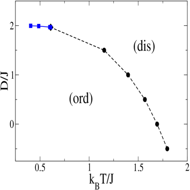
Figure 2: (Color online). Monte Carlo estimates for the locations of the phase boundary of the two- dimensional Blume-Capel model, in the plane of variables $k_{B}T/J$ (abscissa) and $D/J$ (ordinate). Full squares denote first-order transitions, the full diamond denotes the tricritical point ($k_{B}T_{t}/J\approx 0.609,\,D_{t}/J\approx 1.965)$, and full circles denote second-order transitions. Broken straight lines connecting these points are guides to the eye only. The ordered ferromagnetic phase (ord) occurs below the line, and the disordered phase (dis) above it, as indicated. Note that the standard two-dimensional Ising model results in the limit where $D/J$ tends to minus infinity; so its transition is beyond the scale of the diagram.

In addition, part of the bulk phase diagram of the Blume-Capel model has been calculated, by applying again standard Monte Carlo methods 70 but using finite-size scaling for $L\times L$ lattices with periodic boundary conditions in both $x$ and $y$ directions, see Fig. 2. For earlier studies see e.g. 77 ; 78 .

III MONTE CARLO RESULTS ON THE WETTING BEHAVIOR

Motivated by the analysis of Sec. II, we have analyzed the first two moments $\langle|m|\rangle$, $\langle m^{2}\rangle$ and the cumulant 69 ; 70

$$U(T)=1-\langle m^{4}\rangle/[3\langle m^{2}\rangle^{2}]\quad,$$ (46)

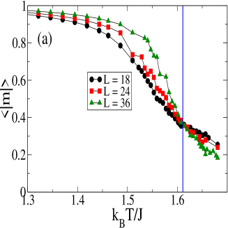
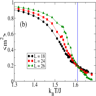
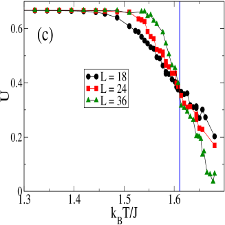
Figure 3: (Color online). Plots of the average absolute value of the magnetization $\langle|m|\rangle$ (a), the magnetization square (b), and the cumulant (c) versus temperature, for the choice $D/J=-\infty$, $H_{1}/J=0.70$, thus all data shown refer to the standard two-dimensional Ising model. The vertical lines indicate the exactly known 19 location of the wetting transition temperature. Curves connecting points are drawn as guides to the eye (also in Figs. 4, 5).

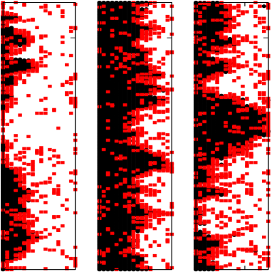
Figure 6: (Color online). Snapshot pictures of the spin configuration of the Blume-Capel model at $D/J=1.5$ and $H_{1}/J=0.7$ for $(L,M)=(18,288)$ at three temperatures: $k_{B}T/J=0.445$ (left), 0.481 (middle) and 0.518 (right). The sites where $S_{i}=-1$ are shown in black, the sites where $S_{i}=0$ are shown in grey (red color online), while sites with $S_{i}=+1$ are left blank. Note that the case $k_{B}T/J=0.481$ is close to the wetting transition.

of the magnetization distribution and plot them versus temperature $T$ for a few typical values of $D/J$, as shown in Figs. 3- 5). As expected, rather well-defined intersection points in all three quantities $\langle|m|\rangle$, $\langle m^{2}\rangle$ and $U(T)$ can be found at the same estimate $k_{B}T_{w}(H_{1})/J$ within reasonably small errors. As always 69 ; 70 , the statistical accuracy is better for $\langle|m|\rangle$ and $\langle m^{2}\rangle$ than for the cumulant. For standard phase transitions in the bulk 70 , $\langle|m|\rangle$ and $\langle m^{2}\rangle$ would not exhibit “universal”, size-independent, intersection points, of course. So, the behavior seen in Figs. 3- 5 is clear evidence for the scaling description of Sec. II, and also the direct observation of configuration snapshots, see e.g. Fig. 6, is compatible with the qualitative picture that was developed (Fig. 1). Note that in the wet phase the average position of the interface is in the middle of the $L\times M$ strip, in between the rows $y=L/2$ and $y=1+L/2$, for $L$ even as chosen here; but due to capillary waves on the scale $M$ in $x-$direction the interface makes excursions of order $\sqrt{M}$ in $y-$direction, which are of the order of $L/2$, for our choice of geometry (Eq. (45)).

On the other hand, in the case shown for $D=-\infty$, i.e. the Ising limit of the Blume-Capel model (Fig. 3), the location of the wetting transition is exactly known 18 , Eq. (I), and highlighted by a vertical straight line. Evidently, the intersection of the curves in Fig. 3 occurs at a temperature compatible with this prediction.

We do expect that the critical wetting transition of the Blume-Capel model falls in the same universality class as for the Ising model. Thus, for the same choice of the generalized aspect ratio $c$, Eq. (45), we expect the same ordinate values of the intersection points of $\langle|m|\rangle$, $\langle m^{2}\rangle$ and $U(T)$, respectively. Within our accuracy, the data are compatible with this expectation.

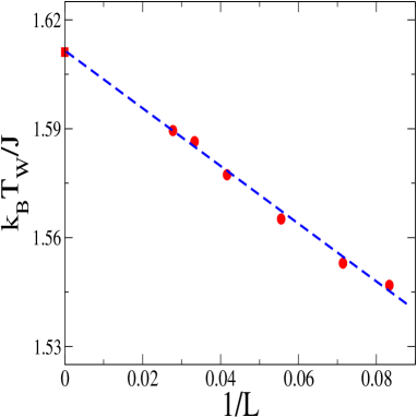
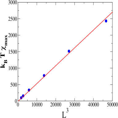
Figure 7: (Color online). a) Extrapolation of the peak position $k_{B}T_{\rm max}/J$ versus $1/L$ (see Eq. (44)) for the case $D/J=-\infty,H_{1}/J=0.7$. The full square indicates the exactly known 19 location of the wetting transition temperature, and the dashed line has been drawn in order to guide the eye. Note that $L^{2}/M=9/8$ (Eq. (45)) is chosen throughout. b) Linear-linear plot of $k_{B}T\chi_{\rm max}$ versus $L^{3}$, for the same choice as used in a), to demonstrate the power law $k_{B}T\chi_{\rm max}\propto L^{3}~{}$ or $(M^{3/2})$, see Eq. 37.

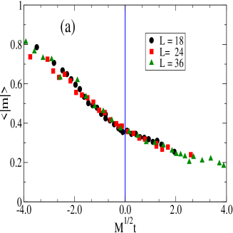
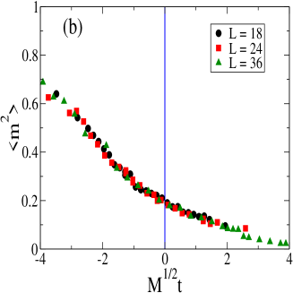
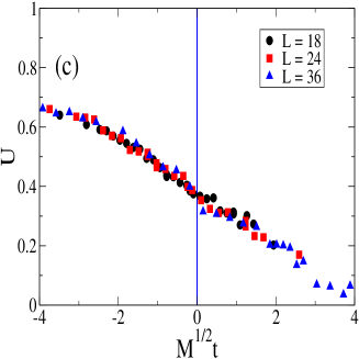
Figure 8: (Color online). Scaling plot of $\langle|m|\rangle_{T}$ (a), $\langle m^{2}\rangle$ (b), and $U$ (c) versus $t\sqrt{M}$ for the same case $D/J=-\infty$, $H_{1}/J=0.7$, and various choices of $L$ (for $L^{2}/M=9/8)$ as indicated in the figure. The vertical line is a reminder that in this case the transition point $t=0$ is known exactly.

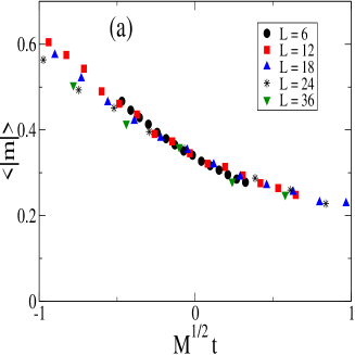
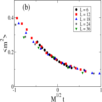
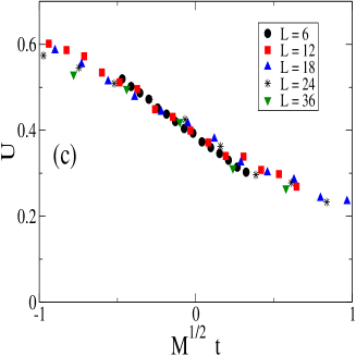
Figure 9: (Color on line). Same as Fig. 8, but for the case $D/J=1.75$, $H_{1}/J=0.85$. The transition point $t=0$ was determined in Fig. 5.

Fig. 7 analysis the scaling of the peak heights and peak locations of the susceptibility $k_{B}T\chi^{\prime}$, cf. Eq. (37) and Eq. (44), respectively. Also, Figs. 8 and  9 present some examples for the “data collapse” on master curves when $\langle|m|\rangle$, $\langle m^{2}\rangle$ and $U$ are plotted as a function of $t\sqrt{M}$ as a test of Eq. (II.3), $\langle|m|\rangle=\tilde{m}(L^{2}/M$, $Mt^{2}\hat{\xi}^{-1}_{||}$) where we used the asymptotic power law for $\xi_{||}$, $\xi_{||}=\hat{\xi}_{||}t^{-\nu_{||}}=\hat{\xi}_{||}t^{-2}$. One sees that a fair data collapse does in fact occur, although deviations due to both statistical errors and systematic effects are present, when $M$ and/or $\xi_{||}$ are not large enough or when data too far away from $T_{w}(H_{1})$ are included. Of course, Figs. 7-9 are just examples only, but representative for the general pattern of behavior. In any case, we do conclude that using such finite-size scaling analyses as presented here one can locate wetting transitions for two dimensional lattice models, such as the Blume-Capel model on the square lattice, with reasonable accuracy.

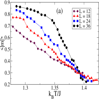
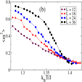
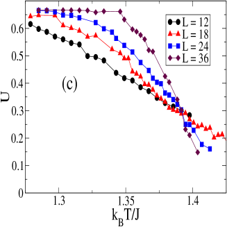
Figure 4: (Color online). Same as Fig. 3, but for $D/J=0.0$, $H_{1}/J=0.55$. From the intersection points one can conclude $k_{B}T_{w}(H_{1})/J=1.393\pm 0.004$, where the error bar merely reflects the scattering of the intersection points of the measured observables.

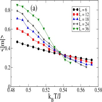
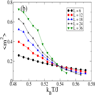
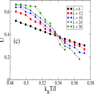
Figure 5: (Color online). Same as Fig. 3, but for $D/J=1.75$, $H_{1}/J=0.85$. From the intersection points one can conclude $k_{B}T_{w}(H_{1})/J=0.538\pm 0.004$, where the error bar merely reflects the scattering of the intersection points of the measured observables.

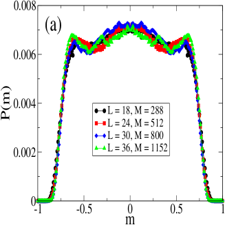
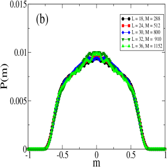
Figure 10: (Color online). (a) Plots of $P_{L,M}(m)$ versus $m$ as obtained for various choices of $L$ and $M$, as indicated, but keeping $L^{2}/M=9/8$ (Eq. (45))and for the case $D=-\infty$. Data obtained for $H_{1}/J=0.70$ and the exactly known 19 location of the wetting transition temperature, namely $k_{B}T_{w}(H_{1})/J\simeq 1.6111$. (b) As in (a) but for the case $D/J=1.50$, and $H_{1}/J=0.70$. The best data collapse of the data is obtained for $k_{B}T_{w}(H_{1})/J=0.792$, in agreement with the intersection points of the quantities $\langle|m|\rangle_{T}$, $\langle m^{2}\rangle_{T}$ and $U(T)$, which are not shown here for the sake of space.

On view of the well-defined intersection points and the data collapse in all three quantities $\langle|m|\rangle$, $\langle m^{2}\rangle$ and $U(T)$ so far studied, figures 3-5 and 8-9, respectively, it is worth to analyze the scaling behavior of the distribution function $P_{L,M}(m)$ of the total magnetization given by equation (27). In fact, since one has $\beta=0$ the prefactor and the third scaling argument are constants. Also, just at $k_{B}T_{w}(H_{1})/J$ (i.e. $t=0$) the second scaling argument vanishes due to the divergence of the correlation length $\xi_{||}$, so that the distribution function depends on the generalized aspect ratio $c=L^{\nu_{||}/\nu_{\bot}}/M$, equation (45), of the sample only. Figures 10 (a) and (b) show plots of $P_{L,M}(m)$ versus $m$ as obtained by keeping $c=9/8$ and for the cases $D/J=-\infty$ and $D/J=1.50$, respectively. It might be expected that the curves of the probability distribution would be independent of $D$, except for normalization corrections due to the different density of vacancies. Since we found that the shape of the probability distribution depends sensitively on $T$, it could be that the qualitative differences between the curves shown in figures 10 (a) and (b) would be due to the uncertainties in the location of $k_{B}T_{w}(H_{1})/J$ for the case $D/J=1.50$.

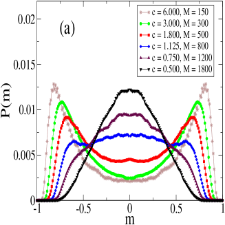
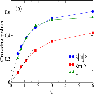
Figure 11: (Color online). (a) Plots of $P_{L,M}(m)$ versus $m$ as obtained for $L=30$ and various choices of $M$, in order to scan a wide range of the generalized aspect ratio $c=L^{2}/M$, as indcated. Data obtained for $D/J=-\infty$, $H_{1}/J=0.70$ and the exactly known 19 location of the wetting transition temperature, namely $k_{B}T_{w}(H_{1})/J\simeq 1.6111$. (b) Intersection points of the quantities $\langle|m|\rangle$, $\langle m^{2}\rangle$, and $U(T)$, versus the sample generalised aspect ratio $c=L^{2}/M$ as obtained for the same parameters as in (a). The dashed lines showing a linear extrapolation to $c=0$ have been drawn for the sake of comparison.

On the other hand, by keeping the temperature, the crystal field, and the surface magnetic field just at the wetting transition point, we have measured the dependence of $P_{L,M}(m)$ on the generalized aspect ratio, for the Ising model, as shown in figure 11 (a). In that figure we choose $L=30$ while $M$ is varied. We recall the non-trivial shapes of the probability distributions that exhibit a single peak around $m=0$ for rather elongated samples (i.e. $c\leq 0.75$), which monotonically crosses over to a bimodal distribution in the limit of more ’cubic’ samples (i.e. $c\geq 1.80$). Also, the generalized aspect ratio selected for our detailed Monte Carlo simulations ($c=9/8$), which can roughly be located within the crossover regime, exhibits not only the central peak, but it also shows the onset of growth of lateral shoulders close to $m\simeq\pm 0.60$. By using the distributions already shown in figure 11 (a) we can also measure the dependence of the crossing points on the generalized aspect ratio of the sample (figure  11 (b)). From this plot it follows that the suitable range of $c$ in order to obtain a reliable intersection point for both $\langle|m|\rangle$ and $U(T)$ in Monte Carlo simulations is rather narrow, say $0.75\leq c\leq 2$, and slightly broader for the case of $\langle m^{2}\rangle$. In order to be able to locate intersections with reasonable accuracy, it is advisable that the cumulant intersection is neither close to zero nor close to its maximun value ($2/3$). It is also reassuring to see that for no shape the distribution at the wetting transition resembles the shape expected for a first-order wetting transition, which would be three delta functions at zero and positive and negative spontaneous magnetization in the thermodynamic limit, and a distribution with three peaks of approximately Gaussian shape in a large but finite system.

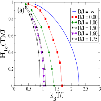
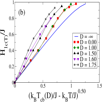
Figure 12: (Color online). a) Plot of $H_{1c}(T)/J$, the inverse function of $k_{B}T_{w}(H_{1})/J$ versus temperature for a range of values of $D/J$, as indicated in the figure. b) Plot of $H_{1c}(T)/J$ versus $(k_{B}T_{cb}(D)/J-k_{B}T/J)^{1/2}$ for a range of value $D/J$, to show that the exponent $\Delta_{1}=1/2$, irrespective of $D/J$, in the region of the second-order transition. In both cases a) and b), the full line corresponds to the exact solution for the case $D/J=-\infty$ given by Eq. (I) 19 .

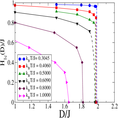
Figure 13: (Color online). Plot of $H_{1c}(T)/J$ versus $D/J$ for the tricritical temperature $(k_{B}T/J=0.609)$, and three temperatures in the region of $k_{B}T/J$ where the transition in the bulk clearly is first order, $k_{B}T/J=0.3045$, $k_{B}T/J=0.406$, and $k_{B}T/J=0.500$, respectively, as indicated. Also, two sets of data corresponding to the range of $k_{B}T/J$ where the transition in the bulk clearly is second order, $k_{B}T/J=0.8000$, and $k_{B}T/J=1.00$, respectively, are shown as indicated. Note that dashed-straight lines connecting the points are drawn as guide to the eye only.

The location of the wetting transitions as a function of two parameters, $H_{1}/J$ and $D/J$, by determining well-defined intersection points still requires extensive computations and hence is a challenging task, Figs. 12 and  13. Since $H_{1c}(J)$ at $k_{B}T_{t}/J=0.609$ decreases only rather slowly with increasing $D$ when one approaches $D_{t}$, it obviously is very difficult to estimate the exponent $\Delta_{1t}$ (Eq. (4) numerically. In mean-field theory, supposed to be exact for $d\geq 4$ we know that $\Delta_{1}=1/2$ and $\Delta_{1t}=1/4$ 47 ; 52 ; 79 ; while in $d=3$ dimensions numerical estimates yielded 26 $\Delta_{1}\approx 0.45$, and we know that in $d=2$ $\Delta_{1}=1/2$ again. So, we see that the exponent $\Delta_{1}$ never deviates much from its mean-field value, if at all. If we speculate the same observation to be true for $\Delta_{1t}$, we would expect that the data in Fig. 13 for $T=T_{t}$ vary as $(1-D/D_{t})^{1/4}$, which is not unreasonable.

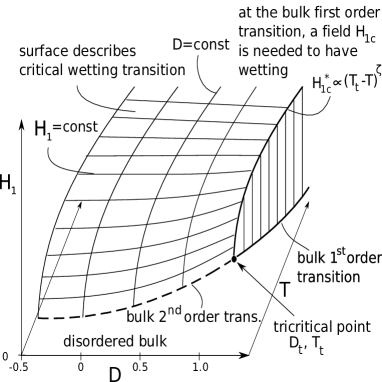
Figure 14: Schematic description of the wetting behavior of the two-dimensional Blume-Capel model in the space of variables $H_{1}$, $D$ and $T$. Complete wetting occurs above the surface of critical wetting transition, which ends at $H_{1}=0$ when the bulk transition is continuous, and at the line $H^{*}_{1c}(T)$ in the region beyond the tricritical point $(D_{t},T_{t})$, where the transition in the bulk is of 1^st order.

We also see that in the region where the transition in the bulk is first order, the wetting transition lines $H_{1c}(D)$ indeed end at nonzero values $H^{*}_{1c}(D)$ at the bulk transition line, and these values decrease as one approaches the tricritical point, qualitatively compatible with Eq. (6). Thus, we can sketch the global wetting behavior as shown schematically in Fig. 14; however, it would be premature to attempt to estimate the exponent $\varsigma$: our data are clearly too limited for this purpose, and we have not tried to extend our study, since we feel the incomplete knowledge on the precise location of the bulk tricritical point 77 ; 78 would hamper such a study.

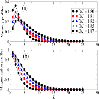
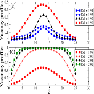
Figure 15: (Color online). Vacancy concentration profiles (a,c,d) and the magnetization profiles (b) plotted as a function of the distance from the wall on which the positive surface field acts, in the case where the majority of the thin strip is in a state of negative magnetization in case (a), (b). Data refer to the lattice with linear dimensions $(L,M)=(24,288)$ and the reduced temperature $k_{B}T/J=0.406$, surface field $|H_{1}|/J=0.91$, and several choices of the parameter $D/J$, as indicated.

As a final problem we consider the enrichment of vacancies at the interface between oppositely magnetized domains in the Blume-Capel model. This problem has been considered earlier by Selke et al. 58 ; 59 ; 60 for the case of free unbound interfaces, while here we consider the extension where the interfaces are confined between competing walls and may undergo a wetting (interface unbinding) transition. Fig. 15 shows plots of the profiles of the vacancy density (a) and the magnetization (b) for a situation of incomplete wetting. One observes a clear enrichment of the vacancies in the interfacial region. The more the interface unbinds from the wall, the more the peak of the vacancy concentration moves away from the wall (Figs. 15 a,b). Note that for the low temperature shown, the magnetization in the bulk tends to $\langle m\rangle=-1$, i.e.  the vacancy concentration inside the bulk is very small.

Close to the wetting transition, the interface gets detached from the wall, and then the interface is located in the middle of the strip, at $z=(L+1)/2$ on average. However, since the interface strongly fluctuates around its average position a straightforward measurement of the vacancy concentration profile would yield an almost horizontal flat curve across the strip. So we have defined a local coarse-graining of the interface, taking segments of length $\Delta x=8$ in the $x$-direction, and determining the local center of mass $z=\tilde{\ell}(x)$ of the interface in each segment, we compute the vacancy distribution in each segment separately, relative to the center in each segment, and superpose the distributions from the individual segments such that their centers coincide. In this way one obtains vacancy profiles with a clear peak in the center of the strip in the wet phase (Fig. 15c). Finally, when one reaches the phase boundary of the bulk, the disordered phase takes over in the film, and the vacancy concentration becomes (almost) unity in the system, except near the boundaries where the surface fields still stabilize layers of up-spins and down-spins, respectively (Fig. 15d). Note, of course, that the details of the curves in Fig. 15c,d do depend on this coarse-graining length $\Delta x$ distinctly.

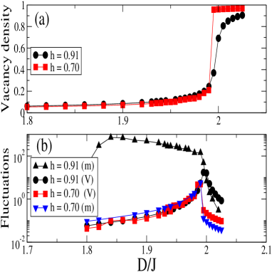
Figure 16: (Color online). Total concentration of vacancies in the system (a) and its fluctuation (b) plotted vs. $D/J$ for $k_{B}T/J=0.406$ and several choices of the surface field $h=|H_{1}|/J$, as indicated. Part(b) includes also the fluctuation of the magnetization $m$ for comparison. The system linear dimensions were again chosen as $(L,M)=(24,288)$.

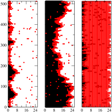
Figure 17: (Color online). Typical snapshot pictures of the spin configurations obtained for $k_{B}T/J=0.406$, $|H_{1}|/J=0.91$ and three values of $D/J:D/J=1.80$ (left panel, refers to an uncompletely wet state), 1.90 (medium panel, wet phase), 2.02 (right panel, disordered phase beyond the first order transition of the bulk). Sites $i$ with $S_{i}=1$ are shown by black dots, sites $i$ with $S_{i}=0$ are shown as grey (b/w) or red (in color) dots, sites $i$ with $S_{i}=-1$ are left blank.

This ambiguity that results depend on the coarse-graining is avoided when one simply computes the average fraction of vacancies in the system (Fig. 16). While for $|H_{1}|$ chosen such that the system is in the incompletely wet state up to the transition in the bulk one sees also a clear jump in the vacancy concentration from a small value to almost unity when this transition in the bulk occurs, a much more rounded behavior is found when wetting at the boundaries occurs. The difference between incompletely wet states and completely wet states is even more pronounced when one studies the magnetization fluctuation: for wet states, this fluctuation is very large for almost all values of $D$ until the transition in the bulk is reached (Fig. 16b). This behavior is corroborated by an examination of snapshot pictures (Fig. 17).

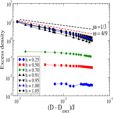
Figure 18: (Color online). Log-log plot of the excess density of the vacancies versus $(D_{\rm coex}-D)/J$ at $k_{B}T/J=0.406$ (where $D_{\rm coex}/J=1.996)$ and different values of the surface field $h=H_{1}/J$. Broken lines show the theoretical slopes 1/3 (expected in the first-order region far off from the tricritical point) and 4/9 (expected at the tricritical point), see also Eq. (9). Chosen lattice size was $(L,M)=(201,400)$.

Finally, Fig. 18 shows an attempt to study the divergence of the interfacial adsorption, that we expect when we approach the bulk transition in the wet phase in the region where a first-order transition occurs. However, it is seen that the effective slope of these data changes slightly when the transition is approached, and also depends on $|H_{1}|/J$. As a consequence, we must conclude that the asymptotic region where a universal exponent could be estimated has not been reached. In view of the strong and slow fluctuations of the interface it is not straightforward to cope with this problem.

IV Conclusions

In this paper, we have presented a Monte Carlo study of the wetting behavior of the two-dimensional Blume-Capel model, mapping out the surface critical field $H_{1w}(T,D)$ where critical wetting occurs for a broad range of parameters $T$ and $D$, both in the region where the transition of the Blume-Capel model in the bulk is of second order (cf. Fig. 12) and where is of first order (cd. Fig. 13). We suggest that $H_{1c}(T,D)$ behaves as $H_{1c}(T,D)\propto(T_{cb}(D)-T)^{1/2}$ for all $D<D_{t}$ and $H_{1c}(T\rightarrow T_{cb}(D))=H_{1c}^{*}(D)$ for $D>D_{t}$, and propose a qualitative phase diagram in the space of the three variables surface field ($H_{1}$), temperature ($T$) and “crystal field” ($D$), as sketched in figure 14. Thus, we present evidence for the universality of the surface critical exponent $\Delta_{1}$ along the critical line of the Blume-Capel model. However, the precise crossover behavior in the inmediate vecinity of the tricritical point $(D_{t},T_{cb}(D_{t}))$ could not yet been studied: first of all, the location of this point needs to be more accurately determined, and also more powerful numerical methods (rather than the straightforward Monte Carlo simulation method just using the Metropolis algorithm) would be required.

Already for the task that we did achieve we encountered the necessity to reconsider the finite-size scaling approach to the study of wetting transitions, Sec. II. We propose that by using a procedure where the linear dimensions $L,M$ of the $L\times M$ strip are varied such that the generalized aspect ratio $c=L^{2}/M$ is kept constant, cf. Eq. (45), it is possible to analyze the data in full analogy to the study of a bulk phase transition, where one uses antisymmetric surface fields ($H_{1}=-H_{L}$). Then, simply the total magnetization $m$ in the system acts like as order parameter, but the appropiate critical exponent is $\beta=0$. Using the exactly known results for the Ising model in the square lattice, which is the limit of the Blume-Capel model for $D\rightarrow\infty$, as a test case, our new finite-size scaling approach is nicely verified. Note that $H_{1c}(T,D\rightarrow\infty)$ and the critical exponents $\nu_{||}=2$, $\nu_{\bot}=1$, $\Delta_{s}=3$, $\alpha_{s}=0$, $\beta_{s}=-1$, and $\gamma_{s}=4$ for critical wetting are known. Then, we propose the corresponding exponents when one treats the transition not as a surface free energy singularity of the semi-infinite system in the limit where the bulk field $H$ tends to zero, but as a bulk singularity of the $L\times M$ system for $H\rightarrow 0$ in the limit $L\rightarrow\infty$, $L^{2}/M=c=$ constant. These expònents are $\alpha=-1$, $\beta=0$ and $\gamma=3$. We have shown that these exponents satisfy all expected scaling relations and we have verified them from our simulations. Use of this formulation of finite-size scaling for critical wetting in $d=2$ dimensions is a convenient and useful tool; it would be interesting to study the extension of this method to $d=3$ dimensions where $\nu_{\bot}=0$ (logarithmic growth) and this extreme shape anisotropy that our method then requires makes the task obviously very much harder.

Since the Blume-Capel model differs from the Ising model by the presence of vacancies as a third component, it is interesting to ask to what extent vacancies get enriched at the interfaces in this situation of interfaces confined by walls. We found that the situation is fully analogous to interfaces between coexisting phases in the bulk: in the second-order region the interfacial adsorption is finite, while in the first-order region the predicted divergence of interfacial adsorption is found.

Of course, there are many cases where by changing a parameter the order of a phase transition in the bulk changes from second to first order, and one can ask how wetting phenomena are affected. We hope that the present work will stimulate further theroretical and experimental studies along such lines.

Acknowledgement: One of as (EVA) received support from the Alexander von Humboldt Foundation and from the Schwerpunkts für Rechnergestützte Forschungsmethoden in den Naturwissenschaften (SRFN), Germany. Also, the support of the the CONICET, ANPCyT and UNLP (Argentina) is greatly acnowledged.

Figure 1: Schematic description of the system geometry and its state slightly below the wetting transition temperature $T_{w}(H_{1})$ such that both $\xi_{||}$ and $\xi_{\bot}$ are much larger than the lattice spacing. Coarse-graining the local magnetization on a length scale intermediate between the lattice spacing and $\xi_{\bot}$, one is left with one coarse-grained contour (the interface) separating the domain with positive magnetization, which was assumed to be the majority domain in the figure, without loss of generality, so the interface is still bound to the lower wall, from the domain with negative magnetization. The sign of the magnetization of the domains is indicated by double arrows. Note that $\xi_{||}\propto\xi^{2}_{\bot}$, and the mean distance of the interface from the nearest boundary also is of the same order as $\xi_{\bot}$. The choice of linear dimensions $L,M$, and of the periodic boundary conditions in $x$-direction (p.b.c.) is indicated.

References

- (1) J.S. Rowlinson and B. Widom, Molecular Theory of Capillarity (Oxford University Press, Oxford, 1982)
- (2) P.G. De Gennes, F. Brochard-Wyart, and D. Queré: Capillarity and Wetting Phenomena: Drops, Bubbles, Pearls, Waves (Springer, Berlin, 2003)
- (3) M. Schön and S. Klapp, Nanoconfined Fluids: Soft Matter Between Two and Three Dimensions (J. Wiley & Sons, New York, 2006)
- (4) I. Brovchenko and A. Oleinikova, Interfacial and Confined Water (Elsevier, Amsterdam, 2008)
- (5) G. Decker and J.B. Schlenoff (eds.) Multilayer Thin Films: Sequential Assembly of Nanocomposite Materials (Wiley-VCH, Weinheim, 2002)
- (6) Y. Champion and H.-J. Fecht (eds.) Nano-Architectured and Nano-Structured Materials (Wiley-VCH, Weinheim, 2004)
- (7) S. Zhang (ed.) Handbook of Nanostructured Thin Films and Coatings, Vol. 1-3 (CRC Press, Boca Rotan, 2010)
- (8) T.M. Squires and S.R. Quake, Rev. Mod. Phys. 77, 977 (2005)
- (9) P.G. De Gennes, Rev. Mod. Phys. 57, 827 (1985)
- (10) D.E. Sullivan and M.M. Telo da Gama, in C. Croxton (ed) Fluid Interfacial Phenomena (Wiley, New York, 1986) p.45
- (11) D.B. Abraham, in C. Domb and J.L. Lebowitz (eds.) Phase Transitions and Critical Phenomena, Vol. 10 (Academic, London, 1986) p.1
- (12) S. Dietrich, in C. Domb and J.L. Lebowitz (eds.) Phase Transitions and Critical Phenomena, Vol. 12 (Academic, London, 1988) p.1.
- (13) M. Schick, in J. Charvolin, J.-F. Joanny, and J. Zinn-Justin (eds.) Liquids at Interfaces (Elsevier, Amsterdam, 1990) p. 415
- (14) G. Forgacs, R. Lipowsky and T.M. Nieuwenhuizen, in C. Domb and J.L. Lebowitz (eds.) Phase Transitions and Critical Phenomana, Vol. 14 (Academic, London, 1991) Chap. 2
- (15) D. Bonn and D. Ross, Rep. Progr. Phys. 64, 1085 (2001)
- (16) D.R. Clarke, M. Rühle, A.P. Tomsia (eds.) Low and High Temperature Wetting: State of the Art; Ann. Revs. Mater. Res., Vol. 38 (Ann. Revs., Palo Alto, 2008)
- (17) D. Bonn, J. Eggers, J. Indekeu, J. Meunier, and E. Rolley, Rev. Mod. Phys. 81, 739 (2009)
- (18) K. Binder, D.P. Landau, and M. Müller, J. Stat. Phys. 110, 1411 (2003)
- (19) D.B. Abraham, Phys. Rev. Lett. 44, 1165 (1980)
- (20) M.E. Fisher and H. Nakanishi, J. Chem. Phys. 75, 5857 (1981)
- (21) H. Nakanishi and M.E. Fisher, Phys. Rev. Lett. 49, 1565 (1982)
- (22) H. Nakanishi and M.E. Fisher, J. Chem. Phys. 78, 3270 (1983)
- (23) K. Binder, D.P. Landau and D.M. Kroll, Phys. Rev. Lett. 56, 2272 (1986)
- (24) D.B. Abraham and E.R. Smith, J. Stat. Phys. 43, 621 (1986)
- (25) K. Binder and D.P. Landau, Phys. Rev. B37, 1745 (1988)
- (26) K. Binder, D.P. Landau, and S. Wansleben, Phys. Rev. B40, 6971 (1989)
- (27) E.V. Albano, K. Binder, D.W. Heermann, and W. Paul, Surf. Sci. 223, 151 (1989)
- (28) E.V. Albano, K. Binder, D.W. Heermann, and W. Paul, J. Stat. Phys. 61, 161 (1990)
- (29) A.O. Parry and R. Evans, Phys. Rev. Lett. 64, 439(1990)
- (30) A.O. Parry and R. Evans, Physica A 181, 250 (1992)
- (31) K. Binder, D.P. Landau, and A.M. Ferrenberg, Phys. Rev. Lett. 74, 298 (1995)
- (32) K. Binder, D.P. Landau, and A.M. Ferrenberg, Phys. Rev. E51, 2823 (1995)
- (33) K. Binder, R. Evans, D.P. Landau, and A.M. Ferrenberg, Phys. Rev. E53, 5023 (1996)
- (34) A. Maciolek and J. Stecki, Phys. Rev. B54, 1128 (1996)
- (35) A. Maciolek, J. Phys. A29, 3837 (1996)
- (36) E. Carlon and A. Drzewinski, Phys. Rev. E57, 2626 (1998)
- (37) E.V. Albano, K. Binder, and W. Paul, J. Phys.:Condens. Matter 12, 2701 (2000)
- (38) A. De Virgiliis, E.V. Albano, M. Müller, and K. Binder, Physics A352, 477 (2005)
- (39) B.J. Schulz, K. Binder, and M. Müller, Phys. Rev. E71, 046705 (2005)
- (40) L. Pang, D.P. Landau, and K. Binder, Phys. Rev. Lett. 106, 236102 (2011)
- (41) L.D. Gelb, K.E. Gubbins, R. Radhakrishnan, and M. Slivinska-Bartkowiak, Rep. Progr. Phys. 63, 1573 (1999)
- (42) E.V. Albano, K. Binder, D.W. Heermann, and W. Paul, J. Chem. Phys. 91, 3700 (1989)
- (43) K. Binder and D.P. Landau, J. Chem. Phys. 96, 1444 (1992)
- (44) O. Dillmann, W. Janke, M. Müller, and K. Binder, J. Chem. Phys. 114, 5823 (2001)
- (45) K. Binder and P.C. Hohenberg, Phys. Rev. B6, 3461 (1972)
- (46) K. Binder and P.C. Hohenberg, Phys. Rev. B9, 2194 (1974)
- (47) K. Binder, in C. Domb and J.L. Lebowitz (eds.) Phase Transitions and Critical Phenomena, Vol. 8 (Academic, London, 1983) p.1.
- (48) L. Onsager, Phys. Rev. 65, 117 (1944)
- (49) M. Blume, Phys. Rev. 141, 517 (1966)
- (50) H.W. Capel, Physica 32, 966 (1966)
- (51) S. Sarbach and I.D. Lawrie, in C. Domb and J.L. Lebowitz (eds.) Phase Transitions and Critical Phenomena, Vol. 9 (Academic, London, 1984) p.1
- (52) K. Binder and D.P. Landau, Surf. Sci. 61, 577 (1976)
- (53) J.L. Cardy, in C. Domb and J.L. Lebowitz (eds.) Phase Transitions and Critical Phenomena, Vo. 11 (Academic, London, 1987) p.55
- (54) R.B. Pearson, Phys. Rev. B22, 2579 (1980)
- (55) B. Nienhuis, J. Phys. A: Math. Gen. 15, 199 (1982)
- (56) H.E. Stanley, An Introduction to Phase Transitions and Critical Phenomena (Oxford Univ. Press, Oxford, 1971)
- (57) K. Binder, in D.G. Pettifor (ed.) Cohesion and Structure of Surfaces (Elsevier, Amsterdam, 1995) p. 121.
- (58) W. Selke and J. Yeomans, J. Phys. A16, 2789 (1983)
- (59) W. Selke, D.A. Huse, and D.M. Kroll, J. Phys. A17, 3019 (1984)
- (60) W. Selke, Surf. Sci. 144, 176 (1984)
- (61) R. Lipowsky, Phys. Rev. B32, 1731 (1985)
- (62) D.M. Kroll, R. Lipowsky, and R.K.P. Zia, Phys. Rev. B32, 1862 (1985)
- (63) A.O. Parry, J.M. Romero-Enrique and A. Lazarides, Phys. Rev. Lett. 93, 086104 (2004)
- (64) A.O. Parry, C. Rascon, N.R. Bernardino, and J.M. Romero-Enrique, J. Phys.: Condens. Matter 18, 6433 (2006); ibid 19, 416105 (2007)
- (65) A.O. Parry, C. Rascon, N.R. Bernardino, and J.M. Romero-Enrique, Phys. Rev. Lett. 100, 136105 (2008)
- (66) A.O. Parry, J.M. Romero-Enrique, N.R. Bernardiono, and J. Rascon, J. Phys.: Condens. Matter 20, 505102 (2008)
- (67) K. Binder and J.S. Wang, J. Stat. Phys. 55, 87 (1989)
- (68) K. Binder, in V. Privman (ed.) Finite Size Scaling and Numerical Simulation of Statistical Systems (World Scientific, Singapore, 1990) p. 173
- (69) S.M. Bhattacharjee and J.F. Nagle. Phys. Rev. A, 31, 3199 (1985)
- (70) S.M. Bhattacharjee and J.J. Rajasekaran. Phys. Rev. A, 44, 6202 (1991)
- (71) K. Binder, Phys. Rev. Lett. 47, 693 (1981)
- (72) K. Binder, Rep. Progr. Phys. 60, 487 (1997)
- (73) L.D.C. Jaubert , J.T. Chalker, P.C.W. Holdsworth, and R. Moessner. Phys. Rev. Lett. 105, 087201 (2010)
- (74) A. Milchev, M. Müller, K. Binder, and D.P. Landau, Phys. Rev. Lett. 90, 136101 (2003)
- (75) A. Milchev, M. Müller, K. Binder, and D.P. Landau, Phys. Rev. E68, 031601 (2003)
- (76) A. Milchev, M. Müller, K. Binder, Europhys. Lett. 70, 348 (2005)
- (77) A. Milchev, M. Müller, and K. Binder, Phys. Rev. E72, 031603 (2005)
- (78) A. DeVirgiliis, E.V. Albano, M. Müller, and K. Binder, J. Phys.: Condens. Matter 17, 4579 (2005)
- (79) A. Winkler, D. Wilms, P. Virnau, and K. Binder, J. Chem. Phys. 133, 164702 (2010)
- (80) D.P. Landau and R.H. Swendsen, Phys. Rev. B33, 7700 (1986)
- (81) J.D. Kimel, S. Black, P. Carter, and Y.L. Wang, Phys. Rev. B35, 3347 (1987)
- (82) W. Speth, Z. Phys. B51, 361 (1983)