Complete Real Time Solution of the General Nonlinear Filtering Problem without Memory

Abstract

It is well known that the nonlinear filtering problem has important applications in both military and civil industries. The central problem of nonlinear filtering is to solve the Duncan-Mortensen-Zakai (DMZ) equation in real time and in a memoryless manner. In this paper, we shall extend the algorithm developed previously by S.-T. Yau and the second author to the most general setting of nonlinear filterings, where the explicit time-dependence is in the drift term, observation term, and the variance of the noises could be a matrix of functions of both time and the states. To preserve the off-line virture of the algorithm, necessary modifications are illustrated clearly. Moreover, it is shown rigorously that the approximated solution obtained by the algorithm converges to the real solution in the $L^{1}$ sense. And the precise error has been estimated. Finally, the numerical simulation support the feasibility and efficiency of our algorithm.

I Introduction

Tracing back to 1960s, two most influential mathematics papers [11], [12] have been published in ASME’s Journal of Basic Engineering. These are so-called Kalman filter (KF) and Kalman-Bucy filter. They addressed a significant question: How does one get accurate estimate from noisy data? The applications of KF are endless, from seismology to bioengineering to econometrics. The KF surpasses the other filtering in, at least, the following two aspects:

• The KF uses each new obervation to update a probability distribution for the state of the system without refering back to any earlier observations. This is so-called “memoryless” or “without memory”.

• The KF makes the decisions of the state on the spot, while the observation data keep coming in. This property is called “real time” application.

Despite its success in many real applications, the limitations on the nonlinearity and Gaussian assumption of the initial probability density of the KF push the mathematicians and scientists to seek the optimal nonlinear filtering. One direction is to modify KF to adapt the nonlinearities. The researchers developed extended Kalman filter (EKF), unscented Kalman filter, ensemble Kalman filter, etc., which can handle weak nonlinearities (that is almost linear). But for serious nonlinearities, they may completely fail. The failure of EKF is shown in our numerical experiment, see the 1D cubic sensor in section VII.A.

Another direction, and also the most popular method nowadays, is the particle filter (PF), refer to as [1], [3] and reference therein. It is developed from sequential Monte Carlo method. On the one hand, the PF is appliable to nonlinear, non-Gaussian state update and observation equations. As the number of particles goes to infinity, the PF estimate becomes asymptotically optimal. On the other hand, it is hard to be implemented as a real time application, due to its essence of Monte Carlo simulation.

Besides the widely used two methods above, the partial differential equaitons (PDE) methods are introduced to the nonlinear filtering in 1960s. These methods are based on the fact that the unnormalized conditional density of the states is the solution of Duncan-Mortensen-Zakai (DMZ) equation, refer to as [6], [16] and [23]. The classical PDE methods could be applied to this stochastic PDE to obtain an approximation to the density. Yet, the main drawback of PDE methods are the intensive computation. It is almost impossible to achieve the “real time” performance. To overcome this shortcoming, the splitting-up algorithm is introduced to move the heavy computation off-line. It is like the Trotter product formula from semigroup theory. This operator splitting algorithm is proposed for the DMZ equation by Bensoussan, Glowinski, and Rascanu [5]. More research articles follow this direction are [9], [15] and [10], etc. Unfortunately, it is pointed out in [5] that the soundness of this algorithm is verified only to the filtering with bounded drift term and observation term ( i.e., $f$ and $h$ in (2.1)). Essentially with the similar idea, Yau and Yau [22] developed a novel algorithm to the “pathwise-robust” DMZ equation (see (2.6)), where the boundedness conditions are weakened by some mild growth conditions on $f$ and $h$. The two nice properties of the KF have also been kept in this algorithm: “without memory” and “real time”. But their algorithm has only been rigorously proved in theory, when the drift term, the observation term ($f$, $h$ in (2.1)) are not explicitly dependent on time, the variance of the noises ($G$ in (2.1)) is the identity matrix, and the noises are standard Brownian motion processes ($S=I_{r\times r}$, $Q=I_{m\times m}$ in (2.1)) .

In this paper, we shall extend the algorithm in [22] to the most general settings of nonlinear filtering problems, in the sense that the drift term, the observation term could explicitly depend on time, the variance of the noises $S$, $Q$ are time-dependent, and $G$ could be a matrix of functions of both time and the states. We shall validate our algorithm under very mild growth conditions on $f$, $h$ and $G$, see (1), (2) and (1). These are essentially time-dependent analogue of those in [22]. First of all, this extension is absolutely necessary. Many real applications have explicit time-dependence in their models, say the target orientation angles estimation from target position/velocity in constant turn model, where the angular velocities are piecewise constant functions in time [18]. Second, this extension is nontrivial from the mathematical point of view. More trickier analysis of PDE is required. For instance, we need to take care of the more general elliptic operator $D_{w}^{2}$, see (2.5), rather than the Laplacian.

This paper is organized in the following. The detailed formulation of our algorithm is described in section II; In section III, we state our main theorems which validate our algorithm in theory. Notations and prelimilary are in section IV. Section V is devoted to the proofs of the main theorems. The lower bound of the density function is investigated in section VI. Numerical simulations are included in section VII. Finally, we arrive the conclusion. The appendices is consisted of the proof of the well-posedness theorem and the proof of an interesting property of the density function.

II Model and Algorithm

The model we are considering is the signal observation model with explicit time-dependence in the drift term, observation term and the variance of the noises:

$$\left\{\begin{aligned} dx_{t}&=f(x_{t},t)dt+G(x_{t},t)dv_{t},\\ dy_{t}&=h(x_{t},t)dt+dw_{t},\end{aligned}\right.$$ (2.1)

where $x_{t}$ and $f$ are $n$-vectors, $G$ is an $n\times r$ matrix, and $v_{t}$ is an $r$-vector Brownian motion process with $E[dv_{t}dv_{t}^{T}]=Q(t)dt$, $y_{t}$ and $h$ are $m$-vectors and $w_{t}$ is an $m$-vector Brownian motion process with $E[dw_{t}dw_{t}^{T}]=S(t)dt$ and $S(t)>0$. We refer to $x_{t}$ as the state of the system at time $t$ with some initial state $x_{0}$ (not necessarily obeying Gaussian distribution) and $y_{t}$ as the observation at time $t$ with $y_{0}=0$. We assume that $\{v_{t},t\geq 0\}$, $\{w_{t},t\geq 0\}$ and $x_{0}$ are independent. For the sake of convenience, let us call this system is the “time-varying” case, while in [22] the “time-invariant” case is studied.

Throughout this paper, we assume that $f$, $h$ and $G$ are $C^{2}$ in space and $C^{1}$ in time. Some growth conditions on $f$ and $h$ are expected to guaratee the existence and uniqueness of the “pathwise-robust” DMZ equation.

The unnormalized density function $\sigma(x,t)$ of $x_{t}$ conditioned on the observation history $Y_{t}=\{y_{s}:0\leq s\leq t\}$ satisfies the DMZ equation (for the detailed formulation, see [6])

$$\left\{\begin{aligned} d\sigma(x,t)&=L\sigma(x,t)dt+\sigma(x,t)h^{T}(x,t)S^{-1}(t)dy_{t}\\ \sigma(x,0)&=\sigma_{0}(x),\end{aligned}\right.$$ (2.2)

where $\sigma_{0}(x)$ is the probability density of the initial state $x_{0}$, and

$$L(\ast)\equiv\frac{1}{2}\sum_{i,j=1}^{n}\frac{\partial^{2}}{\partial x_{i}\partial x_{j}}\left[\left(GQG^{T}\right)_{ij}\ast\right]-\sum_{i=1}^{n}\frac{\partial(f_{i}\ast)}{\partial x_{i}}.$$ (2.3)

In this paper, we don’t solve the DMZ equation directly, due to the following two reasons. On the one hand, the DMZ equation (2.2) is a stochastic partial differential equation due to the term $dy_{t}$. There is no easy way to derive a recursive algorithm to solve this equation. On the other hand, in real applications, one may be more interested in constructing robust state estimators from each observation path, instead of having certain statistical data of thousands of repeated experiments. Here, the robustness means our state esitmator is not sensitive to the observation path. This property is important, since in most of the real applications, the observation arrives and is processed at discrete moments in time. The state estimator is expected to still perform well based on the linear interpolation of the discrete observations, instead of the real continuous observation path. For each “given” observation, making an invertible exponential transformation [19]

$$\sigma(x,t)=\exp{[h^{T}(x,t)S^{-1}(t)y_{t}]}\rho(x,t),$$ (2.4)

the DMZ equation is transformed into a deterministic partial differential equation (PDE) with stochastic coefficients, which we will refer as the “pathwise-robust” DMZ equation

$$\left\{\begin{aligned} \frac{\partial\rho}{\partial t}(x,t)&+\frac{\partial}{\partial t}(h^{T}S^{-1})^{T}y_{t}\rho(x,t)\\ =&\exp{(-h^{T}S^{-1}y_{t})}\left[L-\frac{1}{2}h^{T}S^{-1}h\right]\\ &\cdot[\exp{(h^{T}S^{-1}y_{t})\rho(x,t)}]\\ \rho(x,0)=&\sigma_{0}(x).\end{aligned}\right.$$ (2.5)

Or equivalently,

$$\left\{\begin{aligned} \frac{\partial\rho}{\partial t}(x,t)&=\frac{1}{2}D^{2}_{w}\rho(x,t)+F(x,t)\cdot\nabla\rho(x,t)+J(x,t)\rho(x,t)\\ \rho(x,0)&=\sigma_{0}(x),\end{aligned}\right.$$ (2.6)

where

$$D^{2}_{w}= \sum_{i,j=1}^{n}(GQG^{T})_{ij}\frac{\partial^{2}}{\partial x_{i}\partial x_{j}},$$ (2.7)

$$F(x,t)= \left[\sum_{j=1}^{n}\frac{\partial}{\partial x_{j}}\left(GQG^{T}\right)_{ij}\right.$$

$$\left.+\sum_{j=1}^{n}(GQG^{T})_{ij}\frac{\partial K}{\partial x_{j}}-f_{i}\right]_{i=1}^{n},$$ (2.8)

$$J(x,t) =-\frac{\partial}{\partial t}(h^{T}S^{-1})^{T}y_{t}+\frac{1}{2}\sum_{i,j=1}^{n}\frac{\partial^{2}}{\partial x_{i}\partial x_{j}}\left(GQG^{T}\right)_{ij}$$

$$+\sum_{i,j=1}^{n}\frac{\partial}{\partial x_{i}}\left(GQG^{T}\right)_{ij}\frac{\partial K}{\partial x_{j}}$$

$$+\frac{1}{2}\sum_{i,j=1}^{n}(GQG^{T})_{ij}\left[\frac{\partial^{2}K}{\partial x_{i}\partial x_{j}}+\frac{\partial K}{\partial x_{i}}\frac{\partial K}{\partial x_{j}}\right]$$

$$-\sum_{i=1}^{n}\frac{\partial f_{i}}{\partial x_{i}}-\sum_{i=1}^{n}f_{i}\frac{\partial K}{\partial x_{i}}-\frac{1}{2}(h^{T}S^{-1}h),$$ (2.9)

in which

$$K(x,t)=h^{T}(x,t)S^{-1}(t)y_{t}.$$ (2.10)

The existence and uniqueness of the “pathwise-robust” DMZ equation (2.6) has been investigated by Pardoux [17], Fleming-Mitter [7], Baras-Blankenship-Hopkins [2] and Yau-Yau [21], [22]. The well-posedness is guaranteed, when the drift term $f\in C^{1}$ and the observation term $h\in C^{2}$ are bounded in [17]. Fleming and Mitter treated the case where $f$ and $\nabla f$ are bounded. Baras, Blankenship and Hopkins obtained the well-posedness result on the “pathwise-robust” DMZ equation with a class of unbounded coefficients only in one dimension. In [21], Yau and Yau established the well-posedness result under the condition that $f$, $h$ have at most linear growth. In the appendices of [22], Yau and Yau obtained the existence and uniqueness results in the weighted Sobolev space, where $f$ and $h$ satisfy some mild growth condition. It is necessary to point out that there is a gap in their proof of existence (Theorem A.4). In this paper, we circumvent the gap by more delicate analysis to give a time-dependent analogous well-posedness result to the “pathwise-robust” DMZ equation under some mild growth conditions on $f$ and $h$ in Theorem 4.3.

The exact solution to (2.5) or (2.6), generally speaking, doesn’t have a closed form. So many mathematicians pay their effort on seeking an efficient algorithm to construct a good approximation. In this paper, we will extend the algorithm in [22] to the “time-varying” case (cf. (2.1)). We will not only give the theoretical proof of the soundness of our algorithm, but also illustrate a “time-varying” numerical simulation to support our results. The difficulties are two folds: on one hand, the well-posedness of the “time-invariant” robust DMZ equation, under some conditions, has been investigated by [7], [17], [22], etc., while that in the “time-varying” case hasn’t been established yet; on the other hand, the “time-varying” case will lead to more involved computations and more delicate analysis. For instance, the Laplacian in “time-invariant” case is replaced by a time-dependent elliptic operator $D_{w}^{2}$ in (2.7). Furthermore, the two nice properties of KF, namely “memoryless” and “real time”, are preserved in our algorithm.

Let us assume that we know the observation time sequence $0=\tau_{0}<\tau_{1}<\cdots<\tau_{k}=T$ apriorily. But the observation data $\{y_{\tau_{i}}\}$ at each sampling time $\tau_{i}$, $i=0,\cdots,k$ are unknown until the on-line experiment runs. We call the computation “off-line”, if it can be performed without any on-line experimental data (or say pre-computed); otherwise, it is called “on-line” computations. One only concerns the computational complexity of the on-line computations, since this hinges the success of “real time” application.

Let us denote the observation time sequence as $\mathcal{P}_{k}=\{0=\tau_{0}<\tau_{1}<\cdots<\tau_{k}=T\}$. Let $\rho_{i}$ be the solution of the robust DMZ equation with $y_{t}=y_{\tau_{i-1}}$ on the interval $\tau_{i-1}\leq t\leq\tau_{i}$, $i=1,2,\cdots,k$

$$\left\{\begin{aligned} \frac{\partial\rho_{i}}{\partial t}(x,t)&+\frac{\partial}{\partial t}\left(h^{T}S^{-1}\right)^{T}y_{\tau_{i-1}}\rho_{i}(x,t)\\ =&\exp{\left(-h^{T}S^{-1}y_{\tau_{i-1}}\right)}\left[L-\frac{1}{2}h^{T}S^{-1}h\right]\\ &\cdot\left[\exp{\left(h^{T}S^{-1}y_{\tau_{i-1}}\right)\rho_{i}(x,t)}\right]\\ \rho_{1}(x,0)&=\sigma_{0}(x),\\ \textup{or}\phantom{\rho_{1}(x,0)}&\\ \rho_{i}(x,\tau_{i-1})=&\rho_{i-1}(x,\tau_{i-1}),\quad\textup{for}\ i=2,3,\cdots,k.\end{aligned}\right.$$ (2.11)

Define the norm of $\mathcal{P}_{k}$ by $|\mathcal{P}_{k}|=\sup_{1\leq i\leq k}(\tau_{i}-\tau_{i-1})$. Intuitively, as $|\mathcal{P}_{k}|\rightarrow 0$, we have

$$\sum_{i=1}^{k}\chi_{[\tau_{i-1},\tau_{i}]}(t)\rho_{i}(x,t)\rightarrow\rho(x,t)$$

in some sense, for all $0\leq t\leq T$, where $\rho(x,t)$ is the exact solution of (2.5). That is to say, intuitively, the denser the sampling time sequence is, the more accurate the approximate solution should be obtained. Even though the intuition is shown rigorously to be true, it is impractical to solve (2.11) in the “real time” manner, since the “on-line” data $\{y_{\tau_{i}}\}$, $i=1,\cdots,k$, are contained in the coefficients of (2.11). Therefore, we have to numerically solve the time-consuming PDE on-line, every time after the new observation data coming in. Yet, the proposition below helps to move the heavy computations off-line. This is the key ingredient of the algorithm in [22], so is in ours.

Proposition 2.1

For each $\tau_{i-1}\leq t<\tau_{i}$, $i=1,2,\cdots,k$, $\rho_{i}(x,t)$ satisfies (2.11) if and only if

$$u_{i}(x,t)=\exp{\left[h^{T}(x,t)S^{-1}(t)y_{\tau_{i-1}}\right]}\rho_{i}(x,t),$$ (2.12)

satisfies the Kolmogorov forward equation (KFE)

$$\frac{\partial u_{i}}{\partial t}(x,t)=\left(L-\frac{1}{2}h^{T}S^{-1}h\right)u_{i}(x,t),$$ (2.13)

where $L$ is defined in (2.3).

It is clear that (2.13) is independent of the observation path $\{y_{\tau_{i}}\}_{i=0}^{k}$, and the transformation between $u_{i}$ and $\rho_{i}$ is one-to-one. It is also not hard to see that (2.13) could be numerically solved beforehand. Observe that the operator $\left(L-\frac{1}{2}h^{T}S^{-1}h\right)$ is time-varying, unlike that studied in [22]. Let us denote it as $U(t)$ for short and emphasis its time-dependence. But this doesn’t affect the “off-line” virture of our algorithm. Under certain conditions, $\{U(t)\}_{t\in[0,T]}$ forms a family of strong elliptic operators. Furthermore, the operator $U(t):D(U(t))\subset L^{2}(\mathbb{R}^{n})\rightarrow L^{2}(\mathbb{R}^{n})$ is the infinitesimal generator of the two-parameter semigroup $\mathcal{U}(t,\tau)$, for $t\geq\tau$. In particular, with the observation time sequence known $\{\tau_{i}\}_{i=1}^{k}$, we obtain a sequence of two-parameter semigroup $\{\mathcal{U}(t,\tau_{i-1})\}_{i=1}^{k}$, for $\tau_{i-1}\leq t<\tau_{i}$. Let us take the initial conditions of KFE (2.13) at $t=\tau_{i}$ as a set of complete orthonormal base in $L^{2}(\mathbb{R}^{n})$, say $\{\phi_{l}(x)\}_{l=1}^{\infty}$. We pre-compute the solutions of (2.13) at time $t=\tau_{i+1}$, denoted as $\{\mathcal{U}(\tau_{i+1},\tau_{i})\phi_{l}\}_{l=1}^{\infty}$. These data should be stored in preparation of the on-line computations. Compared with the “time-invariant” case, the price to pay is that the “time-varying” case requires more storage capacity, since $\{\mathcal{U}(\tau_{i+1},\tau_{i})\phi_{l}\}_{l=1}^{\infty}$ differs from each $\tau_{i}$, $i=1,\cdots,k$, and all of them need to be stored. In general, the longer simulation time is the more storage it requires in the “time-varying” case. While the storage of the data is independent of the simulation time in the “time-invariant” case. Nevertheless, it won’t affect the off-line virture of our algorithm.

The on-line computation in our algorithm is consisted of two parts at each time step $\tau_{i-1}$, $i=1,\cdots,k$.

• Project the initial condition $u_{i}(x,\tau_{i-1})\in L^{2}(\mathbb{R}^{n})$ at $t=\tau_{i-1}$ onto the base $\{\phi_{l}(x)\}_{l=1}^{\infty}$, i.e., $u_{i}(x,\tau_{i-1})=\sum_{l=1}^{\infty}\hat{u}_{i,l}\phi_{l}(x)$. Hence, the solution to (2.13) at $t=\tau_{i}$ can be expressed as

  $$u_{i}(x,\tau_{i})= \mathcal{U}(\tau_{i},\tau_{i-1})u_{i}(x,\tau_{i-1})$$

  $$= \sum_{l=1}^{\infty}\hat{u}_{i,l}\left[\mathcal{U}(\tau_{i},\tau_{i-1})\phi_{l}(x)\right],$$ (2.14)

  where $\{\mathcal{U}(\tau_{i},\tau_{i-1})\phi_{l}(x)\}_{l=1}^{\infty}$ have already been computed off-line.

• Update the initial condition of (2.13) at $\tau_{i}$ with the new observation $y_{\tau_{i}}$. Let us specify the observation updates (the initial condition of (2.13) ) for each time step. For $0\leq t\leq\tau_{1}$, the initial condition is $u_{1}(x,0)=\sigma_{0}(x)$. At time $t=\tau_{1}$, when the observation $y_{\tau_{1}}$ is available,

  $$u_{2}(x,\tau_{1}) \overset{\eqref{Rozovsky's reverse transformation}}{=}\exp{[h^{T}(x,\tau_{1})S^{-1}(\tau_{1})y_{\tau_{1}}]}\rho_{2}(x,\tau_{1})$$

  $$\overset{\eqref{Rozovsky's reverse transformation},\eqref{robust DMZ eqn freezed}}{=}\exp{[h^{T}(x,\tau_{1})S^{-1}(\tau_{1})y_{\tau_{1}}]}u_{1}(x,\tau_{1}),$$

  with the fact $y_{0}=0$. Here, $u_{1}(x,\tau_{1})=\sum_{l=1}^{\infty}\hat{u}_{1,l}\left[\mathcal{U}(\tau_{1},0)\phi_{l}(x)\right]$, where $\{\hat{u}_{1,l}\}_{l=1}^{\infty}$ is computed in the previous step, and $\{\mathcal{U}(\tau_{1},0)\phi_{l}(x)\}_{l=1}^{\infty}$ are prepared by off-line computations. Hence, we obtain the initial condition $u_{2}(x,\tau_{1})$ of (2.13) for the next time interval $\tau_{1}\leq t\leq\tau_{2}$. Recursively, the initial condition of (2.13) for $\tau_{i-1}\leq t\leq\tau_{i}$ is

  $$u_{i}(x,\tau_{i-1})= \exp{[h^{T}(x,\tau_{i-1})S^{-1}(\tau_{i-1})(y_{\tau_{i-1}}-y_{\tau_{i-2}})]}$$

  $$\cdot u_{i-1}(x,\tau_{i-1}),$$ (2.15)

  for $i=2,3,\cdots,k$, where $u_{i-1}(x,\tau_{i-1})=\sum_{l=1}^{\infty}\hat{u}_{i-2,l}\left[\mathcal{U}(\tau_{i-1},\tau_{i-2})\phi_{l}(x)\right]$.

The approximation of $\rho(x,t)$, denoted as $\hat{\rho}(x,t)$, is obtained

$$\hat{\rho}(x,t)=\sum_{i=1}^{k}\chi_{[\tau_{i-1},\tau_{i}]}(t)\rho_{i}(x,t),$$ (2.16)

where $\rho_{i}(x,t)$ is obtained from $u_{i}(x,t)$ by (2.12). And $\sigma(x,t)$ could be recovered by (2.4).

A natural question comes to us:

Is $\hat{\rho}(x,t)$, obtained by our algorithm, a good approximation of the exact solution $\rho(x,t)$ to (2.5), for $(x,t)\in\mathbb{R}^{n}\times[0,T]$, as $|\mathcal{P}_{k}|\rightarrow 0$? If it is, then in what sense?

III Statements of the main theorems

In this section, we shall state the main theorems in this paper, which validate our algorithm in theory. Notice that $u_{i}$ in (2.13) and $\rho_{i}$ in (2.11) are one-to-one. Hence, we shall deal with $\rho_{i}$ in the sequel.

We first show that the exact solution $\rho$ of the “pathwise-robust” DMZ equation (2.5) is well approximated by $\rho_{R}$ as $R\rightarrow\infty$, for any $t\in[0,T]$, where $\rho_{R}$ is the solution to (2.5) restricted on $B_{R}$ (the ball centered at the origin with the radius $R$):

$$\left\{\begin{aligned} \frac{\partial\rho_{R}}{\partial t}(x,t)=&\frac{1}{2}D^{2}_{w}\rho_{R}(x,t)+F(x,t)\nabla\rho_{R}(x,t)\\ &+J(x,t)\rho_{R}(x,t)\\ \rho_{R}(x,0)=&\sigma_{0,B_{R}}(x)\\ \rho_{R}(x,t)=&0\qquad\textup{for}\ (x,t)\in\partial B_{R}\times[0,T],\end{aligned}\right.$$ (3.1)

where $D_{w}^{2}$, $F(x,t)$ and $J(x,t)$ are defined in (2.7)-(II) and $\sigma_{0,\Omega}$ is defined as

$$\sigma_{0,\Omega}(x)=\left\{\begin{aligned} &\sigma_{0}(x),\qquad x\in\Omega_{\epsilon}\\ &\textup{smooth},\qquad x\in\Omega\setminus\Omega_{\epsilon}\\ &0,\qquad x\in\mathbb{R}^{n}\setminus\Omega,\end{aligned}\right.$$ (3.2)

in which $\Omega_{\epsilon}=\{x\in\Omega:\ \textup{dist}(x,\partial\Omega)>\epsilon\}$. Next, it is left to show that $\rho_{R}$ is well approximated by the solution obtained by our algorithm restricted on $B_{R}$. In fact, on the time interval $[0,\tau]$, $0<\tau\leq T$. Let us denote the time partition $\mathcal{P}_{k}^{\tau}=\{0=\tau_{0}<\tau_{1}<\cdots<\tau_{k}=\tau\}$. $\rho_{R}(x,\tau)$ is well approximated by $\rho_{k,R}(x,\tau)$, as $k\rightarrow+\infty$, in the $L^{1}$ sense, where $\rho_{k,R}$ is the solution of (2.11) restricted on $B_{R}$.

For the notational convenience, let us denote

$$N(x,t)\equiv -\frac{\partial}{\partial t}\left(h^{T}S^{-1}\right)y_{t}-\frac{1}{2}D_{w}^{2}K$$

$$+\frac{1}{2}D_{w}K\cdot\nabla K-f\cdot\nabla K-\frac{1}{2}\left(h^{T}S^{-1}h\right),$$ (3.3)

where

$$D_{w}\ast=\left[\sum_{j=1}^{n}\left(GQG^{T}\right)_{ij}(x,t)\frac{\partial\ast}{\partial x_{j}}\right]_{i=1}^{n},$$ (3.4)

and $D_{w}^{2}$ and $K$ are defined in (2.7) and (2.10), respectively.

The error estimate between $\rho$ and $\rho_{R}$ is given by the following theorem.

Theorem 3.1

For any $T>0$, let $\rho(x,t)$ be a solution of the “pathwise-robust” DMZ equation (2.6) in $\mathbb{R}^{n}\times[0,T]$. Let $R\gg 1$ and $\rho_{R}$ be the solution to (3.1). Assume the following conditions are satisfied, for all $(x,t)\in\mathbb{R}^{n}\times[0,T]$:

1. $N(x,t)+\frac{3}{2}n\left|\left|GQG^{T}\right|\right|_{\infty}+|f-D_{w}K|\leq C,$ (3.5)

2. $e^{-\sqrt{1+|x|^{2}}}\left[14n\left|\left|GQG^{T}\right|\right|_{\infty}+4\left|f-D_{w}K\right|\right]\leq\tilde{C},$ (3.6)

where $N$, $D_{w}$ and $K$ are defined in (III), (3.4) and (2.10), respectively, and $C$, $\tilde{C}$ are constants possibly depending on $T$. Let $v=\rho-\rho_{R}$, then $v\geq 0$ for all $(x,t)\in B_{R}\times[0,T]$ and

$$\int_{B_{\frac{R}{2}}}v(x,T)\leq\bar{C}e^{-\frac{9}{16}R}\int_{\mathbb{R}^{n}}e^{\sqrt{1+|x|^{2}}}\sigma_{0}(x),$$ (3.7)

where $\bar{C}$ is some constant, which may depend on $T$.

The next theorem tells us that $\rho_{R}$ is well approximated by the solution obtained by our algorithm restricted on $B_{R}$. More generally, $B_{R}$ is replaced by any bounded domain $\Omega\subset\mathbb{R}^{n}$ in the theorem.

Theorem 3.2

Let $\Omega$ be a bounded domain in $\mathbb{R}^{n}$. Assume that

1. $\left|N(x,t)\right|\leq C,$ (3.8)

2. There exists some $\alpha\in(0,1)$, such that

   $$\left|N(x,t)-N(x,t;\bar{t})\right|\leq\tilde{C}|t-\bar{t}|^{\alpha},$$ (3.9)

for all $(x,t)\in\Omega\times[0,T]$, $\bar{t}\in[0,T]$, where $N(x,t)$ is in (III), and $N(x,t;\bar{t})$ denotes $N(x,t)$ with the observation $y_{t}=y_{\bar{t}}$. Let $\rho_{\Omega}(x,t)$ be the solution of (2.6) on $\Omega\times[0,T]$ with $0-$Dirichlet boundary condition:

$$\left\{\begin{aligned} \frac{\partial\rho_{\Omega}}{\partial t}(x,t)=&\frac{1}{2}D^{2}_{w}\rho_{\Omega}(x,t)+F(x,t)\cdot\nabla\rho_{\Omega}(x,t)\\ &+J(x,t)\rho_{\Omega}(x,t)\\ \rho_{\Omega}(x,0)=&\sigma_{0,\Omega}(x)\\ \rho_{\Omega}(x,t)|_{\partial\Omega}=&0,\end{aligned}\right.$$ (3.10)

where $D_{w}^{2}$, $F(x,t)$ and $J(x,t)$ are defined in (2.7)-(II) and $\sigma_{0,\Omega}$ is defined in (3.2). For any $0\leq\tau\leq T$, let $\mathcal{P}_{k}^{\tau}=\{0=\tau_{0}<\tau_{1}<\tau_{2}<\cdots<\tau_{k}=\tau\}$ be a partition of $[0,\tau]$, where $\tau_{i}=\frac{i\tau}{k}$. Let $\rho_{i,\Omega}(x,t)$ be the approximate solution obtained by our algorithm restricted on $\Omega\times[\tau_{i-1},\tau_{i}]$. Or equivalently, $\rho_{i,\Omega}$ is the solution on $\Omega\times[\tau_{i-1},\tau_{i}]$ of the equation

$$\left\{\begin{aligned} \frac{\partial\rho_{i,\Omega}}{\partial t}(x,t)=&\frac{1}{2}D^{2}_{w}\rho_{i,\Omega}(x,t)+F(x,t;\tau_{i-1})\cdot\nabla\rho_{i,\Omega}(x,t)\\ &+J(x,t;\tau_{i-1})\rho_{i,\Omega}(x,t)\\ \rho_{i,\Omega}(x,\tau_{i-1})=&\rho_{i-1,\Omega}(x,\tau_{i-1})\\ \rho_{i,\Omega}(x,t)|_{\partial\Omega}=&0,\end{aligned}\right.$$ (3.11)

for $i=1,2,\cdots,k$, with the convention that $\rho_{1,\Omega}(x,0)=\sigma_{0,\Omega}(x)$. Here, $F(x,t;\tau_{i-1})$, $J(x,t;\tau_{i-1})$ denote $F(x,t)$, $J(x,t)$ with the observation $y_{t}=y_{\tau_{i-1}}$, respectively. Then

$$\rho_{\Omega}(x,\tau)=\lim_{k\rightarrow\infty}\rho_{k,\Omega}(x,\tau),$$

in the $L^{1}$ sense in space and the following estimate holds:

$$\int_{\Omega}|\rho_{\Omega}-\rho_{k,\Omega}|(x,\tau)\leq\bar{C}\frac{1}{k^{\alpha}},$$ (3.12)

where $\bar{C}$ is a generic constant, depending on $T$, $\int_{\Omega}\sigma_{0,\Omega}$. The right-hand side of (3.12) tends to zero as $k\rightarrow\infty$.

IV Notations and preliminary

Throughout the paper, let $\mathbb{Q}_{T}=\mathbb{R}^{n}\times[0,T]$. Let $H^{1}(\mathbb{R}^{n})$ be the Sobolev space, equipped the norm

$$||u(x)||_{1}^{2}=\int_{\mathbb{R}^{n}}(u^{2}+|\nabla_{x}u|^{2})dx.$$

And let $H^{1;1}(\mathbb{Q}_{T})$ be the functional space of both $t$ and $x$, with the norm

$$||v(x,t)||_{1;1}^{2}=\int_{\mathbb{Q}_{T}}(v^{2}+|\nabla_{x}v|^{2}+|\partial_{t}v|^{2})dxdt.$$

The subspace of $H^{1;1}(\mathbb{Q}_{T})$ consisting of functions $v(x,t)$ which have compact supports in $\mathbb{R}^{n}$ for any $t$ is denoted as $H^{1;1}_{0}(\mathbb{Q}_{T})$.

Definition 4.1

The function $u(x,t)$ in $H_{0}^{1;1}(\mathbb{Q}_{T})$ is called a weak solution of the initial value problem

$$\left\{\begin{aligned} &\sum_{i,j=1}^{n}\frac{\partial}{\partial x_{i}}\left(A_{ij}(x,t)\frac{\partial u}{\partial x_{j}}\right)+\sum_{i=1}^{n}B_{i}(x,t)\frac{\partial u}{\partial x_{i}}\\ &\phantom{aaaa}+C(x,t)u=\frac{\partial u}{\partial t},\\ &u(x,0)=u_{0}(x)\end{aligned}\right.$$

if for any function $\Phi(x,t)\in H_{0}^{1;1}(\mathbb{Q}_{T})$ the following relation holds:

$$\int\int_{\mathbb{Q}_{T}} \left[\sum_{i,j=1}^{n}A_{ij}\frac{\partial u}{\partial x_{i}}\frac{\partial\Phi}{\partial x_{j}}\right.$$

$$\left.-\left(\sum_{i=1}^{n}B_{i}\frac{\partial u}{\partial x_{i}}+Cu+\frac{\partial u}{\partial t}\right)\Phi\right]dxdt=0$$

and $u(x,0)=u_{0}(x)$.

We assume that the following conditions hold throughout the paper:

1. The operator $L$ defined in (2.3) is a strong elliptic operator and it is bounded from above on $\mathbb{Q}_{T}$. That is, there exists a constant $\lambda>0$ such that

   $$\lambda|\xi|^{2}\leq\sum_{i,j=1}^{n}(GQG^{T})_{ij}\xi_{i}\xi_{j},$$

   for any $(x,t)\in\mathbb{Q}_{T}$, for any $\xi=(\xi_{1},\xi_{2},\cdots,\xi_{n})\in\mathbb{R}^{n}$. And

   $$||GQG^{T}||_{\infty}=\sup_{(x,t)\in\mathbb{Q}_{T}}|GQG^{T}|_{\infty}<\infty,$$

   where $|\cdot|_{\infty}$ is the sup-norm of the matrix.

2. The initial density function $\sigma_{0}(x)\in H^{1}(\mathbb{R}^{n})$ decays fast enough. To be more specific, we require that

   $$\int_{\mathbb{R}^{n}}e^{\sqrt{1+|x|^{2}}}\sigma_{0}(x)<\infty.$$

IV-A Existence and uniqueness of the non-negative weak solution

For the sake of completeness, we state the existence and uniqueness of the non-negative weak solution to (2.6) on $\mathbb{Q}_{T}$ below.

Theorem 4.3

Under the conditions 1)-2) and the conditions (A.1)-(4) in Theorem A.1, the “pathwise-robust” DMZ equation (2.6) on $\mathbb{Q}_{T}$ with the initial value $\sigma_{0}\in H^{1}(\mathbb{R}^{n})$ admits a non-negative weak solution $\rho\in H^{1;1}(\mathbb{Q}_{T})$. Assume further that the conditions (A.21)-(A.23) in Theorem A.2 are satisfied, then the weak solution $\rho$ on $\mathbb{Q}_{T}$ is unique.

To avoid the distraction from our main theorems, we leave the detailed proof of this theorem in Appendix A.

IV-B Technical lemma

In the proofs of our main theorems, we will repeatedly adopt the following lemma with suitably chosen test functions. Let us state the lemma and sketch the proof here.

Lemma 4.1

Assume that $\rho_{\Omega}$ satisfies the “pathwise-robust” DMZ equation (2.6) on some bounded domain $\Omega\in\mathbb{R}^{n}$, for $0\leq t\leq T$. Then, for any test function $\psi(x)\in C^{\infty}(\Omega)$, we have

$$\frac{d}{dt}\int_{\Omega}\psi\rho_{\Omega}= \frac{1}{2}\int_{\Omega}D_{w}^{2}\psi\rho_{\Omega}+\int_{\Omega}(f-D_{w}K)\cdot\nabla\psi\rho_{\Omega}$$

$$+\int_{\Omega}\psi\rho_{\Omega}N+\frac{1}{2}\int_{\partial\Omega}\psi\left(D_{w}\rho_{\Omega}\cdot\nu\right)$$

$$-\frac{1}{2}\int_{\partial\Omega}\rho_{\Omega}\left(D_{w}\psi\cdot\nu\right)$$

$$+\frac{1}{2}\int_{\partial\Omega}\psi\rho_{\Omega}\sum_{i,j=1}^{n}\frac{\partial}{\partial x_{i}}\left(GQG^{T}\right)_{ij}\nu_{j}$$

$$+\int_{\partial\Omega}\psi\rho_{\Omega}\left(D_{w}K\cdot\nu\right)-\int_{\partial\Omega}\psi\rho_{\Omega}(f\cdot\nu),$$ (4.1)

where $\nu=(\nu_{1},\nu_{2},\cdots,\nu_{n})$ is the exterior normal vector of $\Omega$, and $D_{w}^{2}$, $K$ and $D_{w}$ are defined in (2.7), (2.10) and (3.4), respectively.

Proof:

Multiply $\psi(x)$ on both sides of (2.6) and integrate over the domain $\Omega$, it yields

$$\frac{d}{dt}\int_{\Omega}\psi\rho_{\Omega}= \int_{\Omega}\psi\left[\frac{1}{2}D^{2}_{w}\rho_{\Omega}+F(x,t)\cdot\nabla\rho_{\Omega}+J(x,t)\rho_{\Omega}\right],$$ (4.2)

where $F(x,t)$ and $J(x,t)$ are defined in (II) and (II), respectively. After applying integration by parts to the first two terms on the right-hand side of (4.2), (4.1) is obtained by written in compact notations. ∎

V Proofs of the main theorems

V-A Reduction to the bounded domain case

In this section we shall prove that the solution $\rho$ to the “pathwise-robust” DMZ equation (2.6) in $\mathbb{R}^{n}$ can be well approximated by the solution $\rho_{R}$ of (3.1) in a large ball $B_{R}$. Moreover, the error estimate with respect to the radius $R$ is given explicitly in the $L^{1}$ sense. Let $C$, $\tilde{C}$ and $\hat{C}$ denote the generic constants, which may differ from line to line.

We first show an interesting proposition, which reflects how the density function in the large ball changing with respect to time. It is also an important ingredient of the error estimate in Theorem 3.1.

Proposition 5.2

For any $T>0$, let $\rho_{R}(x,t)$ be a solution of the “pathwise-robust” DMZ equation restricted on $B_{R}$ (3.1). Assume that condition (1) is satisfied. Then

$$\int_{B_{R}}e^{\sqrt{1+|x|^{2}}}\rho_{R}(x,t)\leq e^{Ct}\int_{\mathbb{R}^{n}}e^{\sqrt{1+|x|^{2}}}\sigma_{0}(x).$$ (5.1)

Proof:

Choose the test function in Lemma 4.1 $\psi=e^{\phi_{1}}$ , where ${\phi_{1}}\in C^{\infty}(B_{R})$, $B_{R}=\{x\in\mathbb{R}^{n}:|x|\leq R\}$. Let $\rho_{R}$ be the solution of the “pathwise-robust” DMZ equation (3.1) on the ball $B_{R}$. By Lemma 4.1, we have

$$\frac{d}{dt}\int_{B_{R}}e^{\phi_{1}}\rho_{R}= \int_{B_{R}}e^{\phi_{1}}\rho_{R}\left[\frac{1}{2}\left(D_{w}^{2}{\phi_{1}}+D_{w}{\phi_{1}}\cdot\nabla{\phi_{1}}\right)\right.$$

$$\left.+(f-D_{w}K)\cdot\nabla{\phi_{1}}+N\right]$$

$$+\frac{1}{2}\int_{\partial B_{R}}e^{\phi_{1}}(D_{w}\rho_{R}\cdot\nu).$$ (5.2)

All the boundary integrals in (4.1) vanish, except the first term in (4.1), since $\rho_{R}|_{\partial\Omega}=0$. Moreover, recall that $\rho_{R}\geq 0$ in $B_{R}$ and vanishes on $\partial B_{R}$ implies that $\frac{\partial\rho_{R}}{\partial\nu}|_{\partial B_{R}}\leq 0$. Hence, on $\partial B_{R}$,

$$(D_{w}\rho_{R}\cdot\nu)= \sum_{i=1}^{n}\left[\sum_{j=1}^{n}(GQG^{T})_{ij}\frac{\partial\rho_{R}}{\partial r}\frac{\partial r}{\partial x_{j}}\right]\nu_{i}$$

$$= \frac{\partial\rho_{R}}{\partial r}\left[\sum_{i,j=1}^{n}(GQG^{T})_{ij}\frac{x_{j}}{r}\frac{x_{i}}{r}\right]\leq 0,$$

by the positive definite assumption of $(GQG^{T})$. Thus, (V-A) can be reduced further

$$\frac{d}{dt}\int_{B_{R}}e^{\phi_{1}}\rho_{R}\leq\int_{B_{R}}e^{\phi_{1}}\rho_{R} \left[\frac{1}{2}\left(D_{w}^{2}{\phi_{1}}+D_{w}{\phi_{1}}\cdot\nabla{\phi_{1}}\right)\right.$$

$$\left.+(f-D_{w}K)\cdot\nabla{\phi_{1}}+N\right].$$ (5.3)

Choose ${\phi_{1}}(x)=\sqrt{1+|x|^{2}}$ and estimate the terms containing ${\phi_{1}}$ on the right-hand side of (V-A) one by one:

$$D_{w}^{2}{\phi_{1}}= \sum_{i=1}^{n}\left(GQG^{T}\right)_{ii}\frac{1}{\sqrt{1+|x|^{2}}}$$

$$-\sum_{i,j=1}^{n}\left(GQG^{T}\right)_{ij}\frac{x_{i}x_{j}}{(1+|x|^{2})^{\frac{3}{2}}}$$

$$\leq \left|\left|GQG^{T}\right|\right|_{\infty}\left[\frac{n}{\sqrt{1+|x|^{2}}}+\frac{n|x|^{2}}{(1+|x|^{2})^{\frac{3}{2}}}\right]$$

$$\leq 2n\left|\left|GQG^{T}\right|\right|_{\infty},$$ (5.4)

$$D_{w}{\phi_{1}}\cdot\nabla{\phi_{1}}= \sum_{i,j=1}^{n}\left(GQG^{T}\right)_{ij}\frac{x_{i}x_{j}}{1+|x|^{2}}$$

$$\leq \left|\left|GQG^{T}\right|\right|_{\infty}\frac{\sum_{i,j=1}^{n}x_{i}x_{j}}{1+|x|^{2}}\leq n\left|\left|GQG^{T}\right|\right|_{\infty},$$ (5.5)

and

$$|(f-D_{w}K)\cdot\nabla\phi_{1}|\leq |f-D_{w}K|\cdot\frac{|x|}{\sqrt{1+|x|^{2}}}$$

$$\leq |f-D_{w}K|,$$ (5.6)

where $|\cdot|$ is the Euclidean norm. Substitute the estimate (V-A)-(V-A) back into (V-A), we get

$$\frac{d}{dt} \int_{B_{R}}e^{\phi_{1}}\rho_{R}$$

$$\leq \int_{B_{R}}e^{\phi_{1}}\rho_{R}\left[\frac{3}{2}n\left|\left|GQG^{T}\right|\right|_{\infty}+|f-D_{w}K|+N\right]$$

$$\leq C\int_{B_{R}}e^{\phi_{1}}\rho_{R},$$

by condition (1). Hence,

$$\int_{B_{R}}e^{\phi_{1}}\rho_{R}(x,t)\leq e^{Ct}\int_{B_{R}}e^{\phi_{1}}\rho_{R}(x,0)\leq e^{Ct}\int_{\mathbb{R}^{n}}e^{\phi_{1}}\rho(x,0)$$

$$= e^{Ct}\int_{\mathbb{R}^{n}}e^{\phi_{1}}\sigma_{0}(x),$$

for $0\leq t\leq T$. ∎

We are ready to show Theorem 3.1, i.e. the solution $\rho_{R}$ to (3.1) on $B_{R}$ is a good approximation of $\rho$, the solution to (2.6) in $\mathbb{R}^{n}$.

Proof:

By the maximum principle (cf. Theorem 1, [8]), we have $v=\rho-\rho_{R}\geq 0$ for $(x,t)\in B_{R}\times[0,T]$, since $v|_{\partial B_{R}}\geq 0$ for $0\leq t\leq T$. Let us choose $\psi$ in Lemma 4.1 as

$$\varrho(x)=e^{-{\phi_{2}}(x)}-e^{-R},$$

where ${\phi_{2}}$ is a radial symmetric function such that ${\phi_{2}}(x)|_{\partial B_{R}}=R$, $\nabla{\phi_{2}}|_{\partial B_{R}}=0$ and ${\phi_{2}}$ is increasing in $|x|$. Hence, $\varrho|_{\partial B_{R}}=0$ and $\nabla\varrho|_{\partial B_{R}}=0$. Apply Lemma 4.1 to $v$, taking the place of $\rho_{\Omega}$, with the test function $\psi=\varrho$, we have

$$\frac{d}{dt}\int_{B_{R}}\varrho v= \int_{B_{R}}v\left[\frac{1}{2}D_{w}^{2}\varrho+\left(f-D_{w}K\right)\cdot\nabla\varrho+\varrho N\right]$$

$$= \int_{B_{R}}v\left\{\frac{1}{2}e^{-{\phi_{2}}}\left(D_{w}{\phi_{2}}\cdot\nabla{\phi_{2}}-D_{w}^{2}{\phi_{2}}\right)\right.$$

$$\phantom{\int_{B_{R}}vaa}\left.-e^{-{\phi_{2}}}\left(f-D_{w}K\right)\cdot\nabla{\phi_{2}}+\varrho N\right\}$$

$$= \int_{B_{R}}v\varrho\left[-\frac{1}{2}D_{w}^{2}{\phi_{2}}+\frac{1}{2}D_{w}{\phi_{2}}\cdot\nabla{\phi_{2}}\right.$$

$$\phantom{\int_{B_{R}}vaa}\left.-\left(f-D_{w}K\right)\cdot\nabla{\phi_{2}}+N\right]$$

$$+e^{-R}\int_{B_{R}}e^{\sqrt{1+|x|^{2}}}v\left[e^{-\sqrt{1+|x|^{2}}}\right.$$

$$\phantom{e^{-R}\int}\cdot\left(-\frac{1}{2}D_{w}^{2}{\phi_{2}}+\frac{1}{2}D_{w}{\phi_{2}}\cdot\nabla{\phi_{2}}\right.$$

$$\phantom{e^{-R}\int_{B_{R}}\cdot(}\left.\left.-\left(f-D_{w}K\right)\cdot\nabla{\phi_{2}}\right)\right]$$

$$\triangleq \int_{B_{R}}v\varrho\mathrm{I_{1}}+e^{-R}\int_{B_{R}}e^{\sqrt{1+|x|^{2}}}v\mathrm{I_{2}}.$$

Let us choose $\phi_{2}(x)$ in $\varrho(x)$ to be $\phi_{2}(x)=R\vartheta(\frac{|x|^{2}}{R^{2}})$, where $\vartheta(x)=1-(1-x)^{2}$. It is easy to check that $\phi_{2}(x)$ satisfies all the conditions we mentioned before. Direct computations yield, for any $x\in B_{R}$, $R>>1$,

$$\left|D_{w}^{2}{\phi_{2}}\right|= \left|\sum_{i,j=1}^{n}\left(GQG^{T}\right)_{ij}\left(-\frac{8x_{i}x_{j}}{R^{3}}\right)\right.$$

$$\left.+\sum_{i=1}^{n}\left(GQG^{T}\right)_{ii}\frac{4}{R}\left(1-\frac{|x|^{2}}{R^{2}}\right)\right|$$

$$\leq \left|\left|GQG^{T}\right|\right|_{\infty}\left(\frac{8n|x|^{2}}{R^{3}}+\frac{4n}{R}\right)\leq 12n\left|\left|GQG^{T}\right|\right|_{\infty},$$ (5.7)

$$\left|D_{w}{\phi_{2}}\cdot\nabla{\phi_{2}}\right|= \left|\left(1-\frac{|x|^{2}}{R^{2}}\right)^{2}\sum_{i,j=1}^{n}\left(GQG^{T}\right)_{ij}\frac{4x_{i}}{R}\frac{4x_{j}}{R}\right|$$

$$\leq 16n\left|\left|GQG^{T}\right|\right|_{\infty},$$ (5.8)

and

$$\left|\left(f-D_{w}K\right)\cdot\nabla{\phi_{2}}\right|= \left|\left(f-D_{w}K\right)\frac{4x}{R}\left(1-\frac{|x|^{2}}{R^{2}}\right)\right|$$

$$\leq 4\left|f-D_{w}K\right|.$$ (5.9)

It follows that

$$\sup_{B_{R}}|\mathrm{I_{1}}|\leq 14n\left|\left|GQG^{T}\right|\right|_{\infty}+4\left|f-D_{w}K\right|+N\leq C,$$

by condition (1). Similarly,

$$\sup_{B_{R}}|\mathrm{I_{2}}|\leq \sup_{B_{R}}\left[e^{-\sqrt{1+|x|^{2}}}\left(14n\left|\left|GQG^{T}\right|\right|_{\infty}\right.\right.$$

$$\phantom{\sup_{B_{R}}[e^{-\sqrt{1+|x|^{2}}}(}\left.\left.+4\left|f-D_{w}K\right|\right)\right]$$

$$\leq \tilde{C},$$

by condition (2). In the view of Proposition 5.2, one gets

$$\frac{d}{dt}\int_{B_{R}}\varrho v\leq C\int_{B_{R}}\varrho v+e^{-R}\tilde{C}\int_{B_{R}}e^{\sqrt{1+|x|^{2}}}\rho$$

$$\leq C\int_{B_{R}}\varrho v+e^{-R+\hat{C}T}\tilde{C}\int_{\mathbb{R}^{n}}e^{\sqrt{1+|x|^{2}}}\sigma_{0}(x).$$ (5.10)

Multiply $e^{-Ct}$ on both sides of (V-A) yields

$$\frac{d}{dt}\left[e^{-Ct}\int_{B_{R}}\varrho v\right]\leq e^{-R+\hat{C}T-Ct}\tilde{C}\int_{\mathbb{R}^{n}}e^{\sqrt{1+|x|^{2}}}\sigma_{0}(x).$$

Integrate from $0$ to $T$ and multiply $e^{CT}$ on both sides gives us

$$\int_{B_{R}}\varrho v(x,T)\leq ||v(x,0)||_{\infty}e^{CT}\int_{B_{R}}\varrho dx$$

$$+\frac{e^{CT}-1}{C}e^{-R+\hat{C}T}\tilde{C}\int_{\mathbb{R}^{n}}e^{\sqrt{1+|x|^{2}}}\sigma_{0}(x),$$

where $v(x,0)=\sigma_{0}-\sigma_{0,R}$. Recall that $\varrho(x)=e^{-R\left[-\left(|x|^{2}/R^{2}-1\right)^{2}+1\right]}-e^{-R}$, $|x|\leq R$, we arrive the following estimates:

$$\int_{B_{R}}\varrho\leq\int_{B_{R}}\left(1-e^{-R}\right)\leq CR^{n}$$

and

$$\int_{B_{R}}\varrho v(x,T)\geq \int_{B_{\frac{R}{2}}}\left(e^{-R\left[-\left(|x|^{2}/R^{2}-1\right)^{2}+1\right]}-e^{-R}\right)v(x,T)$$

$$\geq \frac{1}{2}e^{-\frac{7}{16}R}\int_{B_{\frac{R}{2}}}v(x,T).$$

It is easy to see that $||v(x,0)||_{\infty}\int_{B_{R}}\varrho\leq C(n)\epsilon R^{n}$ is arbitrarily small, since $\epsilon$ is independent of $R$. It yields that

$$\int_{B_{\frac{R}{2}}}v(x,T)\leq Ce^{-\frac{9}{16}R}\int_{\mathbb{R}^{n}}e^{\sqrt{1+|x|^{2}}}\sigma_{0}(x),$$ (1.28)

where $C$ is a generic constant, depending on $T$. ∎

By refining the proofs of Proposition 5.2 and Theorem 3.1, we obtain an interesting property of the density function $\rho(x,t)$. It asserts that $\rho$ captures almost all the density in a large ball. And we could give an precise estimate of the density outside the large ball.

Theorem 5.4

Let $\rho(x,t)$ be a solution of the “pathwise-robust” DMZ equation (2.6) in $\mathbb{Q}_{T}$. Assume that

1. Condition (1) is satisfied;

2. A stronger version of condition (2) is valid. To be more precise,

   $$e^{-\frac{1}{2}\sqrt{1+|x|^{2}}}\left[16n\left|\left|GQG^{T}\right|\right|_{\infty}+4\left|f-D_{w}K\right|\right]\leq C,$$ (5.11)

   for all $(x,t)\in\mathbb{Q}_{T}$.

Then

$$\int_{|x|\geq R}\rho(x,T)\leq Ce^{-\frac{1}{2}\sqrt{1+R^{2}}}\int_{\mathbb{R}^{n}}e^{\sqrt{1+|x|^{2}}}\sigma_{0}(x),$$ (5.12)

where $C$ is a generic constant, which depends on $T$.

To avoid the distraction, we leave the detailed proof in Appendix B.

V-B $L^{1}$ convergence

In this section, we shall show that, for any $0<\tau\leq T$, with the partition $\mathcal{P}_{k}^{\tau}=\{0=\tau_{0}<\tau_{1}<\cdots<\tau_{k}=\tau\}$, the $L^{1}$ convergence of $\rho_{k,R}(x,\tau)$ to $\rho_{R}(x,\tau)$ holds, as $k\rightarrow+\infty$, where $\rho_{k,R}$ is the solution of (3.11) obtained by our algorithm, and $\rho_{R}$ is the solution to (3.1). For the clarity, we state the technique lemma will be used in the proof of Theorem 3.2 below.

Lemma 5.2

(Lemma 4.1, [22]) Let $\Omega$ be a bounded domain in $\mathbb{R}^{n}$ and let $v:\overline{\Omega}\times[0,T]\rightarrow\mathbb{R}$ be a $C^{1}$ function. Assume that $v(x,t)=0$ for $(x,t)\in\partial\Omega\times[0,T]$. Let $\Omega_{t}^{+}=\{x\in\Omega:v(x,t)\geq 0\}$. Then

$$\frac{d}{dt}\int_{\Omega_{t}^{+}}v(x,t)=\int_{\Omega_{t}^{+}}\frac{\partial v}{\partial t}(x,t),$$

for almost all $t\in[0,T]$.

Proof:

For the notational convenience, we omit the subscript $\Omega$ for $\rho_{\Omega}$ and $\rho_{i,\Omega}$ in this proof. Let $\Omega_{t}^{+}=\{x\in\Omega:\rho(x,t)-\rho_{i}(x,t)\geq 0\}$. Apply Lemma 4.1 to $(\rho-\rho_{i})$ taking place of $\rho_{\Omega}$, with the test function $\psi\equiv 1$, we have

$$\frac{d}{dt}\int_{\Omega_{t}^{+}}(\rho-\rho_{i})\leq \int_{\Omega_{t}^{+}}(\rho-\rho_{i})N(\cdot,t)$$

$$+\int_{\Omega_{t}^{+}}\rho_{i}[N(\cdot,t)-N(\cdot,t;\tau_{i-1})],$$ (5.1)

by Lemma 5.2. All the boundary integrals vanish, except $\int_{\partial\Omega_{t}^{+}}D_{w}(\rho-\rho_{i})\cdot\nu$, since $(\rho-\rho_{i})|_{\partial\Omega_{t}^{+}}=0$. Moreover, $\int_{\partial\Omega_{t}^{+}}D_{w}(\rho-\rho_{i})\cdot\nu\leq 0$, due to the similar argument for $\int_{\partial B_{R}}D_{w}\rho\cdot\nu\leq 0$ in Proposition 5.2. Combine the conditions (1) and (3.9), (V-B) can be controlled by

$$\frac{d}{dt}\int_{\Omega_{t}^{+}}(\rho-\rho_{i})\leq C\int_{\Omega_{t}^{+}}(\rho-\rho_{i})+\tilde{C}(t-\tau_{i-1})^{\alpha}\int_{\Omega}\rho.$$ (5.2)

To estimate $\int_{\Omega}\rho$, we apply Lemma 4.1 to $\rho$, with the test function $\psi\equiv 1$, we get

$$\frac{d}{dt}\int_{\Omega}\rho\leq\int_{\Omega}\rho N\leq C\int_{\Omega}\rho,$$

which implies

$$\int_{\Omega}\rho\leq C\int_{\Omega}\sigma_{0,\Omega},$$ (5.3)

where $C$ is a generic constant, depending on $T$, for all $0\leq t\leq T$. Thus,

$$\frac{d}{dt}\int_{\Omega_{t}^{+}}(\rho-\rho_{i})\leq C\int_{\Omega_{t}^{+}}(\rho-\rho_{i})+\tilde{C}(t-\tau_{i-1})^{\alpha}\int_{\Omega}\sigma_{0,\Omega}.$$

Multiply $e^{-\tilde{C}(t-\tau_{i-1})}$ on both sides and integrate from $\tau_{i-1}$ to $t$, we get

$$\int_{\Omega_{t}^{+}}(\rho-\rho_{i})(x,t)\leq e^{\tilde{C}(t-\tau_{i-1})}\int_{\Omega_{\tau_{i-1}}^{+}}(\rho-\rho_{i})(x,\tau_{i-1})$$

$$+C\frac{(t-\tau_{i-1})^{1+\alpha}}{1+\alpha}e^{\tilde{C}(t-\tau_{i-1})},$$

where $C$ is a constant, which depends on $T$, $\int_{\Omega}\sigma_{0,\Omega}$. Similarly, one can also get, for $\Omega_{t}^{-}=\{x\in\Omega:\,\rho(x,t)-\rho_{i}(x,t)<0\}$, that

$$\int_{\Omega_{t}^{-}}(\rho_{i}-\rho)(x,t)\leq e^{\tilde{C}(t-\tau_{i-1})}\int_{\Omega_{\tau_{i-1}}^{-}}(\rho_{i}-\rho)(x,\tau_{i-1})$$

$$+C\frac{(t-\tau_{i-1})^{1+\alpha}}{1+\alpha}e^{\tilde{C}(t-\tau_{i-1})}.$$

Consequently, we have

$$\int_{\Omega}|\rho-\rho_{i}|(x,t)$$

$$\leq e^{\tilde{C}(t-\tau_{i-1})}\left[\int_{\Omega}|\rho-\rho_{i}|(x,\tau_{i-1})+C\frac{(t-\tau_{i-1})^{1+\alpha}}{1+\alpha}\right]$$

$$\leq e^{\tilde{C}(t-\tau_{i-1})}\left[\int_{\Omega}|\rho-\rho_{i-1}|(x,\tau_{i-1})+C\frac{(t-\tau_{i-1})^{1+\alpha}}{1+\alpha}\right],$$ (5.4)

since $\rho_{i}(x,\tau_{i-1})=\rho_{i-1}(x,\tau_{i-1})$, for $i=1,2,\cdots,k$. Applying (V-B) recursively, we obtain

$$\int_{\Omega}|\rho-\rho_{k}|(x,\tau_{k})$$

$$\leq e^{\tilde{C}(\tau_{k}-\tau_{k-1})}\left[\int_{\Omega}|\rho-\rho_{k-1}|(x,\tau_{k-1})+C\frac{(\tau_{k}-\tau_{k-1})^{1+\alpha}}{1+\alpha}\right]$$

$$\leq e^{\tilde{C}T}\int_{\Omega}|\rho-\rho_{0}|(x,0)$$

$$+\frac{C}{1+\alpha}[(\tau_{k}-\tau_{k-1})^{1+\alpha}e^{\tilde{C}(\tau_{k}-\tau_{k-1})}$$

$$\phantom{+\frac{2c_{6}}{1+\alpha}[}+(\tau_{k-1}-\tau_{k-2})^{1+\alpha}e^{\tilde{C}(\tau_{k}-\tau_{k-2})}$$

$$\phantom{+\frac{2c_{6}}{1+\alpha}[}+\cdots+(\tau_{1}-\tau_{0})^{1+\alpha}e^{\tilde{C}(\tau_{k}-\tau_{0})}]$$

$$= \frac{C}{1+\alpha}\frac{T^{1+\alpha}}{k^{1+\alpha}}\left(e^{\tilde{C}\frac{T}{k}}+e^{\tilde{C}\frac{2T}{k}}+\cdots+e^{\tilde{C}\frac{kT}{k}}\right)\leq\frac{C}{k^{\alpha}},$$

where $C$ is a constant, which depends on $\alpha$, $T$ and $\int_{\Omega}\sigma_{0,\Omega}$. It is clear that $\int_{\Omega}|\rho-\rho_{k}|\rightarrow 0$, as $k\rightarrow\infty$. ∎

VI Lower bound estimate of density function

It is well-known that solving the “pathwise-robust” DMZ equation numerically is not easy because it is easily vanishing. We are also interested in whether the lower bound of the density function could be derived in the case where the drift term $f$ and the observation term $h$ are with at most the polynomial growth. The theorem below gives this lower bound:

Theorem 6.5

Let $\rho_{R}$ be the solution of (3.1), the “pathwise-robust” DMZ equation on $B_{R}$. Assume that

1. $f(x,t)$ and $h(x,t)$ have at most polynomial growth in $|x|$, for all $t\in[0,T]$;

2. For any $0\leq t\leq T$, there exists positive integer $m$ and positive constants $C^{\prime}$ and $C^{\prime\prime}$ independent of $R$ such that the following two conditions hold on $\mathbb{R}^{n}$:

   (a) $$\frac{|x|^{m-2}}{2}\left[nm(m-2)\left|\left|GQG^{T}\right|\right|_{\infty}\right.$$

   $$\phantom{\frac{|x|^{m-2}}{2}[}\left.+m\,\textup{Tr}\left(GQG^{T}\right)\right]$$

   $$-m|x|^{m-2}(f-D_{w}K)\cdot x+N(x,t)\geq-C^{\prime};$$ (6.1)

   (b) $$\left|n\left|\left|GQG^{T}\right|\right|_{\infty}\left(\frac{1}{2}m^{2}|x|^{2m-2}\right.\right.$$

   $$\phantom{|n\left|\left|GQG^{T}\right|\right|_{\infty}(}\left.-m\left(\frac{1}{2}m-1\right)|x|^{m-2}\right)$$

   $$-\frac{1}{2}m\,\textup{Tr}\left(GQG^{T}\right)|x|^{m-2}$$

   $$\left.-m(f-D_{w}K)\cdot x|x|^{m-2}\right|$$

   $$\leq \frac{1}{2}nm(m+1)\left|\left|GQG^{T}\right|\right|_{\infty}|x|^{2m-2}+C^{\prime\prime},$$ (6.2)

   where $\textup{Tr}(*)$ is the trace of $*$.

3. Condition (1) is satisfied.

Then for any $R_{0}<R$,

$$\int_{B_{R_{0}}}\zeta\rho_{R}(x,T)$$

$$\geq \frac{e^{(C-C^{\prime})T-R_{0}^{m}}}{C^{\prime}}\left(\frac{1}{2}nm(m+1)\left|\left|GQG^{T}\right|\right|_{\infty}R_{0}^{2m-2}+C^{\prime\prime}\right)$$

$$\cdot\left(1-e^{C^{\prime}T}\right)\int_{B_{R}}\sigma_{0,R}(x)+e^{-C^{\prime}T}\int_{B_{R_{0}}}\zeta\sigma_{0,R}(x),$$

where $\zeta(x)=e^{-\xi(x)}-e^{-\xi(R_{0})}$, $\xi(x)=|x|^{m}$.

In particular, the solution $\rho$ of the “pathwise-robust” DMZ equation (2.5) on $\mathbb{R}^{n}$ has the estimate

$$\int_{\mathbb{R}^{n}}e^{-|x|^{m}}\rho(x,T)\geq e^{-C^{\prime}T}\int_{\mathbb{R}^{n}}e^{-|x|^{m}}\sigma_{0}(x).$$

Proof:

Apply Lemma 4.1 to $\rho_{R}$ with the test function $\psi$ to be $\zeta=e^{-\xi(x)}-e^{-\xi(R_{0})}$, where $\xi(x)$ is an increasing function in $|x|$, we have

$$\frac{d}{dt}\int_{B_{R_{0}}}\zeta\rho_{R}=\int_{B_{R_{0}}}\rho_{R}\left[\frac{1}{2}D_{w}^{2}\zeta+\left(f-D_{w}K\right)\cdot\nabla\zeta+\zeta N\right].$$

All the boundary integrals vanish, since $\zeta|_{\partial B_{R}}=\rho_{R}|_{\partial B_{R}}=0$. Direct computations yield that

$$\frac{d}{dt}\int_{B_{R_{0}}}\zeta\rho_{R}$$

$$= \int_{B_{R_{0}}}\rho_{R}e^{-\xi(R_{0})}$$

$$\cdot\left\{\frac{1}{2}\frac{\xi^{\prime 2}(r)}{r^{2}}\sum_{i,j=1}^{n}\left(GQG^{T}\right)_{ij}x_{i}x_{j}-\frac{\xi^{\prime}(r)}{r}(f-D_{w}K)\cdot x\right.$$

$$\phantom{aa}-\frac{1}{2}\sum_{i,j=1}^{n}\left(GQG^{T}\right)_{ij}\left[\left(\xi^{\prime\prime}(r)-\frac{\xi^{\prime}(r)}{r}\right)\frac{x_{i}x_{j}}{r^{2}}\right]$$

$$\phantom{aa}\left.-\frac{1}{2}\textup{Tr}\left(GQG^{T}\right)\frac{\xi^{\prime}(r)}{r}\right\}$$

$$+\int_{B_{R_{0}}}\zeta\rho_{R}\left[\frac{1}{2}D_{w}\xi\cdot\nabla\xi-\frac{1}{2}D_{w}^{2}\xi-(f-D_{w}K)\cdot\nabla\xi+N\right]$$

$$\triangleq \mathrm{I_{3}}+\int_{B_{R_{0}}}\zeta\rho_{R}[\mathrm{I_{4}}].$$

Let $\xi(r)=r^{m}$, where $r=|x|$, $m$ is some positive integer sufficiently large. Through elementary computations, we get

$$\mathrm{I_{4}}$$

$$= \frac{1}{2}\frac{\xi^{\prime 2}(r)}{r^{2}}\sum_{i,j=1}^{n}\left(GQG^{T}\right)_{ij}x_{i}x_{j}$$

$$-\frac{1}{2}\left[m(m-2)r^{m-4}\sum_{i,j=1}^{n}\left(GQG^{T}\right)_{ij}x_{i}x_{j}\right.$$

$$\phantom{-\frac{1}{2}[}\left.+mr^{m-2}\textup{Tr}\left(GQG^{T}\right)\right]-mr^{m-2}(f-D_{w}K)\cdot x+N$$

$$\geq -\frac{1}{2}\left[nm(m-2)\left|\left|GQG^{T}\right|\right|_{\infty}+m\,\textup{Tr}\left(GQG^{T}\right)\right]r^{m-2}$$

$$-mr^{m-2}(f-D_{w}K)\cdot x+N\geq C^{\prime},$$

where $C^{\prime}$ is a positive constant independent of $R_{0}$, by condition (2). For large enough $m$, we have

$$|\mathrm{I_{3}}| \leq e^{-R_{0}^{m}}$$

$$\cdot\int_{B_{R}}\left|n\left|\left|GQG^{T}\right|\right|_{\infty}\left[\frac{1}{2}m^{2}r^{2m-2}-m\left(\frac{1}{2}m-1\right)r^{m-2}\right]\right.$$

$$\phantom{\int_{B_{R}}|}\left.-\frac{1}{2}m\,\textup{Tr}\left(GQG^{T}\right)r^{m-2}-m(f-D_{w}K)\cdot xr^{m-2}\right|\rho_{R}$$

$$\leq e^{-R_{0}^{m}}\left(\frac{1}{2}nm(m+1)\left|\left|GQG^{T}\right|\right|_{\infty}R_{0}^{2m-2}+C^{\prime\prime}\right)\int_{B_{R}}\rho_{R}$$

$$\leq\left(\frac{1}{2}nm(m+1)\left|\left|GQG^{T}\right|\right|_{\infty}R_{0}^{2m-2}+C^{\prime\prime}\right)$$

$$\phantom{\leq 11}\cdot e^{CT-R_{0}^{m}}\int_{B_{R}}\sigma_{0,R}\triangleq\gamma(R_{0}).$$

The last inequality follows by the similar argument of (5.3). Hence,

$$\frac{d}{dt}\int_{B_{R_{0}}}\zeta\rho_{R}\geq-\gamma(R_{0})-C^{\prime}\int_{B_{R_{0}}}\zeta\rho_{R}.$$

This implies

$$\int_{B_{R_{0}}}\zeta\rho_{R}(x,T)$$

$$\geq e^{-C^{\prime}T}\int_{B_{R_{0}}}\zeta\sigma_{0,R}(x)+\frac{\gamma(R_{0})}{C^{\prime}}\left(e^{-C^{\prime}T}-1\right)$$

$$\geq e^{-C^{\prime}T}\int_{B_{R_{0}}}\zeta\sigma_{0,R}(x)$$

$$+\left(\frac{1}{2}nm(m+1)\left|\left|GQG^{T}\right|\right|_{\infty}R_{0}^{2m-2}+C^{\prime\prime}\right)$$

$$\phantom{+a}\cdot\frac{e^{(C-C^{\prime})T-R_{0}^{m}}}{C^{\prime}}\left(1-e^{C^{\prime}T}\right)\int_{B_{R}}\sigma_{0,R}(x).$$ (6.3)

Let $R_{0}\rightarrow\infty$, we have

$$\int_{\mathbb{R}^{n}}e^{-|x|^{m}}\rho(x,T)\geq e^{-C^{\prime}T}\int_{\mathbb{R}^{n}}e^{-|x|^{m}}\sigma_{0}(x).$$

∎

VII Numerical simulations

In this section, we shall apply our algorithm to both “time-invariant” case and “time-varying” case. The numerical simulations support our theorems. In our implementation, we adopt the Hermite spectral method (HSM) to get the approximate solution of (2.13). Thus, the basis functions $\{\phi_{l}\}_{l=1}^{\infty}$ in (• ‣ II) are choosen to be the generalized Hermite functions $\{H_{n}^{\alpha,\beta}(x)\}_{n=0}^{\infty}$. We refer the interested readers to the detailed definitions in [14].

For $N>0$, let us denote $\mathcal{R}_{N}$ the subspace spanned by the first $N$ generalized Hermite functions:

$$\mathcal{R}_{N}= \textup{span}\{H_{0}^{\alpha,\beta}(x),\cdots,H_{N}^{\alpha,\beta}(x)\}.$$

The formulation of HSM to (2.13) in 1-dimension is to find $u_{N}(x,t)\in\mathcal{R}_{N}$ such that

$$\left\{\begin{aligned} \langle\partial_{t}u_{N}(x,t),\varphi\rangle=&-\frac{1}{2}\langle\partial_{x}[(GQG^{T})u_{N}],\partial_{x}\varphi\rangle\\ &+\langle fu_{N},\partial_{x}\varphi\rangle-\frac{1}{2}\langle(h^{T}S^{-1}h)u_{N},\varphi\rangle\\ u_{N}(x,0)=&P_{N}u_{0}(x),\end{aligned}\right.$$ (7.4)

for any $\varphi\in\mathcal{R}_{N}$, where $\langle\cdot,\cdot\rangle$ denotes the scalar product in $L^{2}(\mathbb{R})$ and $P_{N}$ is the projection operator such that $P_{N}:\,L^{2}(\mathbb{R})\rightarrow\mathcal{R}_{N}$. Write the solution $u_{N}\in\mathcal{R}_{N}$ in the form

$$u_{N}(x,t)=\sum_{n=0}^{N}a_{n}(t)H_{n}^{\alpha,\beta}(x),$$

and take the test function $\varphi\in\mathcal{R}_{N}$ in (7.4) to be $H_{n}^{\alpha,\beta}$, $n=0,\cdots,N$. From (7.4) and the properties of generalized Hermite functions, $\vec{a}(t):=(a_{0}(t),a_{1}(t),\cdots,a_{N}(t))^{T}$ satisfies the ODE

$$\partial_{t}\vec{a}(t)=A\vec{a}(t),$$ (7.5)

where $A$ is a $(N+1)\times(N+1)$ matrix, may depend on $t$, if $G$, $Q$, $f$ or $h$ is explicitly time-dependent. This ODE can be precomputed. The only difference between “time-varying” case and “time-invariant” case is that it costs much more memory to store the off-line data in the “time-varying” case, as we explained before in section II. Nevertheless, it doesn’t change the off-line virture of our algorithm. We refer the interested readers of the implementation to [14], and we shall omit the technical details in this paper.

Once $u_{N}$ at each step is obtained, $\hat{\rho}$ can be recovered by (2.12). The conditional expectation of the state $x_{t}$ is computed by definition

$$\mathbb{E}\left[x,\{y_{\tau}\}_{0\leq\tau\leq t}\right](t)=\frac{\int_{\mathbb{R}}x\hat{\rho}(x,t)dx}{\int_{\mathbb{R}}\hat{\rho}(x,t)dx}.$$

VII-A “time-invariant” case: the 1D cubic sensor

Let us consider the following model

$$\left\{\begin{aligned} dx_{t}&=dv_{t}\\ dy_{t}&=x_{t}^{3}dt+dw_{t},\end{aligned}\right.$$

where $x_{t}$, $y_{t}\in\mathbb{R}$, $v_{t}$, $w_{t}$ are scalar Brownian motion processes with $E[dv_{t}^{T}dv_{t}]=1$, $E[dw_{t}^{T}dw_{t}]=1$. The 1D Kolmogorov forward equation (2.13) here is

$$u_{t}=\frac{1}{2}u_{xx}-\frac{1}{2}x^{6}u,$$ (7.6)

at each time step. We assume the inital density function $u_{0}(x)=e^{-x^{4}/4}$ and the updated initial data are

$$u_{i}(x,\tau_{i})=e^{x^{3}\cdot dy_{t}}u_{i-1}(x,\tau_{i}).$$

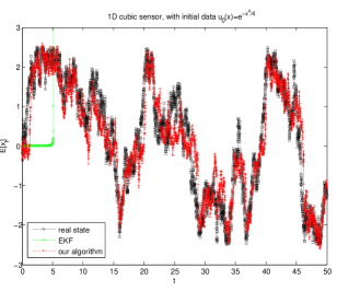
Figure 1: 1D cubic sensor, with the initial condition $u_{0}(x)=e^{-\frac{x^{4}}{4}}$. Black: real state; Green: extended Kalman filter; Red: our algorithm.

In Figure 1, we see that our algorithm tracks the state’s expectation very well, while the extended Kalman filter (EKF) completely fails around $t=5$. The total simulation time is $T=50$, and the update time step is $dt=\tau_{i+1}-\tau_{i}=0.01$. It costs our algorithm only around $4.88s$ to finish the simulation, i.e. the updated time is less than $10^{-3}s$.

VII-B “time-varying” case: the 1D almost linear sensor

The 1D almost linear sensor we are considering is

$$\left\{\begin{aligned} dx_{t}=&[1+0.1\cos{(20\pi t)}]dv_{t}\\ dy_{t}=&x_{t}[1+0.25\cos{(x_{t})}]dt+dw_{t},\end{aligned}\right.$$ (7.7)

where $x_{t}$, $y_{t}\in\mathbb{R}$, $v_{t}$, $w_{t}$ are scalar Brownian motion processes with $E[dv_{t}^{T}dv_{t}]=E[dw_{t}^{T}dw_{t}]=1$. The Kolmogorov forward equation (2.13) in this example is

$$u_{t}=\frac{1}{2}[1+0.1\cos{(20\pi t)}]^{2}u_{xx}-\frac{1}{2}x^{2}[1+0.25\cos{(x)}]^{2}u,$$

with the initial data $u_{0}(x)=e^{-x^{2}/2}$ and the updated initial data

$$u_{i}(x,\tau_{i})=e^{x^{2}[1+0.25\cos{(x)}]\cdot dy_{t}}u_{i-1}(x,\tau_{i}),$$

$i=1,2,\cdots,k$. In Figure 2, our algorithm tracks the state’s expectation at least as well as the EKF. The total simulation time is $T=60$, and the update time step is $dt=\tau_{i+1}-\tau_{i}=0.01$. It costs our algorithm only around $3.17s$ to complete the simulatoin, i.e. the updated time is less than $5\times 10^{-4}s$.

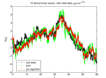
Figure 2: 1D “time-varying” almost linear sensor, with the initial condition $u_{0}(x)=e^{-\frac{x^{2}}{2}}$. Black: real state; Green: extended Kalman filter; Red: our algorithm.

VIII Conclusion

In this paper, we extend the algorithm developed in [22] to the most general nonlinear filterings. We theoretically verified that under very mild growth conditions on the drift term and the observation term, the unique non-negative weak solution $\rho$ of its associated “pathwise-robust” DMZ equation can be approximated by the solution $\rho_{R}$ of the DMZ equation restricted on a large ball $B_{R}$ with 0-Dirichlet boundary condition. The error of this approximation tends to zero exponentially as the radius of the ball $R$ approaching infinity. Moreover, $\rho_{R}$ can be efficiently approximated by our algorithm. We show that the approximate solution $\hat{\rho}_{R}$ obtained by our algorithm converges to $\rho_{R}$ in the $L^{1}$ sense for all $t\in[0,T]$, as the partition of time becomes finer, and a precise error estimate of this convergence is given explicitly. Equally important, our algorithm preserves the two advantages of KF: “memoryless” and “real time”. We also give the detail explanation of the off-line virture of our algorithm in the formulation. Numerical experiments support the feasibility and efficiency of our algorithm.

Appendix A Existence and uniqueness of the solution

Before we show the existence of the weak solution, we shall give a priori estimations of up to the first order derivative of the solution to the robust DMZ equation on $B_{R}\times[0,T]$.

Theorem A.1

Consider the “pathwise-robust” DMZ equation (3.1) on $\mathbb{Q}_{R}:=B_{R}\times[0,T]$, where $B_{R}=\{x\in\mathbb{R}^{n}:|x|\leq R\}$ is a ball of radius $R$. Assume that

$$\left\|\frac{d}{dt}(GQG^{T})\right\|_{\infty}<\infty,$$ (A.1)

for all $t\in[0,T]$. Suppose there exists a positive function $g(x)$ on $\mathbb{R}^{n}$ such that for all $t\in[0,T]$, $g$ and $\tilde{g}\triangleq g+\log{|D_{w}J|}$ satisfy

1. $\left|D_{w}g+\frac{1}{2}\nabla(GQG^{T})-F\right|^{2}+2\lambda_{1}J\leq C,$ (A.2)

2. $D_{w}^{2}g+2D_{w}g\cdot\nabla g+2[\nabla(GQG^{T})-F]\cdot\nabla g+\frac{1}{2}\nabla^{2}(GQG^{T})-\textup{div}F+J\leq C,$ (A.3)

3. $D_{w}^{2}\tilde{g}+2D_{w}\tilde{g}\cdot\nabla\tilde{g}+2[\nabla(GQG^{T})-F]\cdot\nabla\tilde{g}+\frac{1}{2}\nabla^{2}(GQG^{T})-\textup{div}F+J\leq C,$ (A.4)

4. $\int_{\mathbb{R}^{n}}e^{2\tilde{g}}\sigma^{2}(x)\leq C\quad\textup{and}\quad\int_{\mathbb{R}^{n}}e^{2g}D_{w}\sigma\cdot\nabla\sigma\leq C,$ (A.5)

where $C$ is a generic constant, which may differ from line to line, and $\nabla(*)=\left[\sum_{i=1}^{n}\frac{\partial(*)_{ij}}{\partial x_{i}}\right]_{j=1}^{n}$, $\nabla^{2}(*)=\sum_{i,j=1}^{n}\frac{\partial^{2}(*)_{ij}}{\partial x_{i}\partial x_{j}}$. Then, for $0\leq t\leq T$,

$$\int_{B_{R}}e^{2g}\rho_{R}^{2}(x,t)dx\leq e^{Ct}\int_{B_{R}}e^{2g}\sigma^{2}(x)dx,$$ (A.6)

$$\int_{B_{R}}e^{2g}D_{w}\rho_{R}(x,t)\cdot\nabla\rho_{R}(x,t)dx$$

$$\leq e^{Ct}\int_{B_{R}}e^{2g}D_{w}\sigma(x)\cdot\nabla\sigma(x)dx+Ce^{Ct}\int_{B_{R}}e^{2\tilde{g}}\sigma^{2}(x)dx,$$ (A.7)

where $D_{w}$ and $J(x,t)$ is defined in (3.4)and (II), respectively.

Remark A.1

The conditions in Theorem A.1 are easily checked, if the drift terms $h(x)$ and $f(x)$ are at most polynomial growth in $r=|x|$. However, in general, the existence of such $g$ is not always available.

Proof: Let $g$ be some positive function on $\mathbb{R}^{n}$.

$$\frac{d}{dt}\int_{B_{R}}e^{2g}\rho_{R}^{2}= \int_{B_{R}}e^{2g}\rho_{R}D_{w}^{2}\rho_{R}+2\int_{B_{R}}e^{2g}\rho_{R}(F\cdot\rho_{R})$$

$$+2\int_{B_{R}}e^{2g}J\rho_{R}^{2}$$

$$\triangleq \mathrm{I}+\mathrm{II}+\mathrm{III}.$$ (A.8)

Apply integration by parts to $\mathrm{I}$ and $\mathrm{II}$ in (A)

$$\mathrm{I}= -2\int_{B_{R}}\rho_{R}e^{2g}D_{w}g\cdot\nabla\rho_{R}-\int_{B_{R}}e^{2g}D_{w}\rho_{R}\cdot\nabla\rho_{R}$$

$$-\int_{B_{R}}e^{2g}\rho_{R}\nabla(GQG^{T})\cdot\nabla\rho_{R}$$

$$\leq -2\int_{B_{R}}\rho_{R}e^{2g}D_{w}g\cdot\nabla\rho_{R}-\int_{B_{R}}e^{2g}\rho_{R}\nabla(GQG^{T})\cdot\nabla\rho_{R}$$

$$\triangleq\mathrm{I_{1}}+\mathrm{I_{2}}.$$

Integration by parts further, we have

$$\mathrm{I_{1}}= 4\int_{B_{R}}e^{2g}\rho_{R}^{2}D_{w}g\cdot\nabla g+2\int_{B_{R}}e^{2g}\rho_{R}D_{w}g\cdot\nabla\rho_{R}$$

$$+2\int_{B_{R}}e^{2g}\rho_{R}^{2}\nabla(GQG^{T})\cdot\nabla g+2\int_{B_{R}}e^{2g}\rho_{R}^{2}D_{w}^{2}g.$$ (A.9)

Notice that the second term of the right-hand side of (A) is $-\mathrm{I_{1}}$, we have

$$\mathrm{I_{1}}= 2\int_{B_{R}}e^{2g}\rho_{R}^{2}D_{w}g\cdot\nabla g$$

$$+\int_{B_{R}}e^{2g}\rho_{R}^{2}[\nabla(GQG^{T})\cdot\nabla g+D_{w}^{2}g].$$ (A.10)

The similar argument applies to $\mathrm{I_{2}}$:

$$\mathrm{I_{2}}= \int_{B_{R}}e^{2g}\rho_{R}^{2}\nabla(GQG^{T})\cdot\nabla g$$

$$+\frac{1}{2}\int_{B_{R}}e^{2g}\rho^{2}_{R}\nabla^{2}(GQG^{T}).$$ (A.11)

Thus,

$$\mathrm{I}\leq \int_{B_{R}}e^{2g}\rho_{R}^{2}\left[D_{w}^{2}g+2D_{w}g\cdot\nabla g\right.$$ (A.12)

$$\phantom{\int_{B_{R}}e^{2g}\rho_{R}^{2}[a}\left.+2\nabla(GQG^{T})\cdot\nabla g+\frac{1}{2}\nabla^{2}(GQG^{T})\right].$$ (A.13)

The same trick of $\mathrm{I_{1}}$ applies to $\mathrm{II}$ in (A), we obtain

$$\mathrm{II}=-\int_{B_{R}}e^{2g}\rho_{R}^{2}[2F\cdot\nabla g+\textup{div}F].$$ (A.14)

Substitute (A.12) and (A.14) back to (A), we obtain

$$\frac{d}{dt} \int_{B_{R}}e^{2g}\rho_{R}^{2}$$

$$\leq \int_{B_{R}}e^{2g}\rho_{R}^{2}\left\{D_{w}^{2}g+2D_{w}g\cdot\nabla g+2[\nabla(GQG^{T})-F]\cdot\nabla g\right.$$

$$\phantom{\int_{B_{R}}e^{2g}\rho_{R}^{2}[}\left.+\frac{1}{2}\nabla^{2}(GQG^{T})-\textup{div}F+J\right\}$$

$$\leq C\int_{B_{R}}e^{2g}\rho_{R}^{2},$$

by condition (2). (A.6) follows directly from Gronwall’s inequality. To show (A.1), we consider

$$\frac{d}{dt} \int_{B_{R}}e^{2g}D_{w}\rho_{R}\cdot\nabla\rho_{R}$$

$$= \int_{B_{R}}e^{2g}\sum_{i,j=1}^{n}\frac{d}{dt}(GQG^{T})_{ij}\frac{\partial\rho_{R}}{\partial x_{i}}\frac{\partial\rho_{R}}{\partial x_{j}}$$

$$+2\int_{B_{R}}e^{2g}\sum_{i,j=1}^{n}(GQG^{T})_{ij}\frac{\partial}{\partial x_{i}}\left(\frac{\partial\rho_{R}}{\partial t}\right)\frac{\partial\rho_{R}}{\partial x_{j}}$$

$$\triangleq \mathrm{IV}+\mathrm{V}.$$ (A.15)

Due to condition (A.1), $\mathrm{IV}$ of (A) turns out to be

$$\mathrm{IV}\leq \frac{1}{2}\left\|\frac{d}{dt}(GQG^{T})\right\|_{\infty}\int_{B_{R}}e^{2g}\sum_{i,j=1}^{n}\left[\left(\frac{\partial\rho_{R}}{\partial x_{i}}\right)^{2}+\left(\frac{\partial\rho_{R}}{\partial x_{j}}\right)^{2}\right]$$

$$=n\left\|\frac{d}{dt}(GQG^{T})\right\|_{\infty}\int_{B_{R}}e^{2g}|\nabla\rho_{R}|^{2}$$

$$\leq \frac{n}{\lambda_{1}}\left\|\frac{d}{dt}(GQG^{T})\right\|_{\infty}\int_{B_{R}}e^{2g}D_{w}\rho_{R}\cdot\nabla\rho_{R},$$ (A.16)

since $D_{w}\rho_{R}\cdot\nabla\rho_{R}\geq\lambda_{1}|\nabla\rho_{R}|^{2}$. Next, $\mathrm{V}$ in (A) is

$$\mathrm{V}= -2\int_{B_{R}}e^{2g}[(2D_{w}g+\nabla(GQG^{T}))\cdot\nabla\rho_{R}+D_{w}^{2}\rho_{R}]$$

$$\phantom{-2\int_{B_{R}}e^{2g}[}\cdot\left(\frac{1}{2}D_{w}^{2}\rho_{R}+F\cdot\nabla\rho_{R}+J\rho_{R}\right)$$

$$= -\int_{B_{R}}e^{2g}\left\{D_{w}^{2}\rho_{R}+\left[D_{w}g+\frac{1}{2}\nabla(GQG^{T})+F\right]\cdot\nabla\rho_{R}\right\}^{2}$$

$$+\int_{B_{R}}e^{2g}\left[D_{w}g+\frac{1}{2}\nabla(GQG^{T})-F\right]^{2}|\nabla\rho_{R}|^{2}$$

$$-2\int_{B_{R}}e^{2g}[D_{w}^{2}\rho_{R}+(2D_{w}g+\nabla(GQG^{T}))\cdot\nabla\rho_{R}]J\rho_{R}$$

$$\leq \int_{B_{R}}e^{2g}\left[D_{w}g+\frac{1}{2}\nabla(GQG^{T})-F\right]^{2}|\nabla\rho_{R}|^{2}$$

$$-2\int_{B_{R}}e^{2g}[D_{w}^{2}\rho_{R}+(2D_{w}g+\nabla(GQG^{T}))\cdot\nabla\rho_{R}]J\rho_{R}.$$ (A.17)

Notice that

$$\int_{B_{R}}e^{2g}D_{w}^{2}\rho_{R}J\rho_{R}$$

$$= -\int_{B_{R}}e^{2g}\left[2(D_{w}g\cdot\nabla\rho_{R})J\rho_{R}+JD_{w}\rho_{R}\cdot\nabla\rho_{R}\right.$$

$$\phantom{-\int_{B_{R}}e^{2g}[}\left.+(D_{w}\rho_{R}\cdot\nabla J)\rho_{R}+\nabla(GQG^{T})\cdot\nabla\rho_{R}J\rho_{R}\right].$$ (A.18)

Take (A) into account, $\mathrm{V}$ becomes

$$\mathrm{V}\leq \int_{B_{R}}e^{2g}$$

$$\cdot\left\{\frac{1}{\lambda_{1}}\left\{\left[D_{w}g+\frac{1}{2}\nabla(GQG^{T})-F\right]^{2}+1\right\}+2J\right\}$$

$$\cdot D_{w}\rho_{R}\cdot\nabla\rho_{R}+\int_{B_{R}}e^{2g}|D_{w}J|^{2}\rho_{R}^{2}.$$ (A.19)

Combine (A) and (A), we have

$$\frac{d}{dt} \int_{B_{R}}e^{2g}D_{w}\rho_{R}\cdot\nabla\rho_{R}$$

$$\leq \int_{B_{R}}e^{2g}\left\{\frac{1}{\lambda_{1}}\left\{n\left\|\frac{d}{dt}(GQG^{T})\right\|_{\infty}\right.\right.$$

$$\phantom{\int_{B_{R}}e^{2g}}\left.\left.+\left[D_{w}g+\frac{1}{2}\nabla(GQG^{T})-F\right]^{2}+1\right\}+2J\right\}$$

$$\phantom{\int_{B_{R}}e^{2g}}\cdot D_{w}\rho_{R}\cdot\nabla\rho_{R}$$

$$+\int_{B_{R}}e^{2g}|D_{w}J|^{2}\rho_{R}^{2}.$$ (A.20)

By conditions (1)-(4), the estimate (A.1) follows immediately. $\Box$

Proof of existence in Theorem 4.3: Let $R_{k}$ be a sequence of positive number such that $\lim_{k\rightarrow\infty}R_{k}=\infty$. Let $\rho_{k}(x,t)$ be the solution of the “pathwise-robust” DMZ equation (3.1) on $B_{R_{k}}\times[0,T]$, where $B_{R_{k}}=\{x\in\mathbb{R}^{n}:|x|\leq R_{k}\}$ is a ball of radius $R_{k}$. In view of Theorem A.1, the sequence $\{\rho_{k}\}$ is a bounded set in $H_{0}^{1;1}(\mathbb{Q}_{R_{k}})$. Thus, there exists a subsequence $\{\rho_{k^{\prime}}\}$ which is weakly convergent to $\rho$. Moreover, $\rho$ has the weak derivative $\frac{\partial\rho}{\partial x_{i}}\in L^{2}(\mathbb{Q}_{R_{k}})$, and $\frac{\partial\rho_{k^{\prime}}}{\partial x_{i}}$ weakly tends to it. Now we claim that the weak derivative $\frac{\partial\rho}{\partial t}$ exists. To see this, let $\Phi(x,t)\in H_{0}^{1;1}(\mathbb{Q}_{R_{k}})$, then

$$\iint_{\mathbb{Q}_{R_{k}}}\frac{1}{2}\sum_{i,j=1}^{n}(GQG^{T})_{ij}\frac{\partial\Phi}{\partial x_{j}}\frac{\partial\rho}{\partial x_{i}}$$

$$\phantom{\iint_{\mathbb{Q}_{R_{k}}}}+\left[\sum_{i=1}^{n}\left(\sum_{j=1}^{n}\frac{\partial(GQG^{T})_{ij}}{\partial x_{j}}-F_{i}\right)\frac{\partial\rho}{\partial x_{i}}-J\rho\right]\Phi$$

$$= \lim_{k^{\prime}\rightarrow\infty}\iint_{\mathbb{Q}_{R_{k}}}\frac{1}{2}\sum_{i,j=1}^{n}(GQG^{T})_{ij}\frac{\partial\Phi}{\partial x_{j}}\frac{\partial\rho_{k^{\prime}}}{\partial x_{i}}$$

$$+\left[\sum_{i=1}^{n}\left(\sum_{j=1}^{n}\frac{\partial(GQG^{T})_{ij}}{\partial x_{j}}-F_{i}\right)\frac{\partial\rho_{k^{\prime}}}{\partial x_{i}}-J\rho_{k^{\prime}}\right]\Phi$$

$$= -\lim_{k^{\prime}\rightarrow\infty}\iint_{\mathbb{Q}_{R_{k}}}\frac{\partial\rho_{k^{\prime}}}{\partial t}\Phi=\lim_{k^{\prime}\rightarrow\infty}\iint_{\mathbb{Q}_{R_{k}}}\rho_{k^{\prime}}\frac{\partial\Phi}{\partial t}$$

$$= \iint_{\mathbb{Q}_{R_{k}}}\rho\frac{\partial\Phi}{\partial t}.$$

Clearly, $\rho(x,0)=\lim_{k^{\prime}\rightarrow\infty}\rho_{k^{\prime}}(x,0)=\sigma_{0}(x)$.

Theorem A.2

Assume further that for some $c>0$,

$$\sup_{0\leq t\leq T}\int_{\mathbb{R}^{n}}e^{cr}\rho^{2}(x,t)dx<\infty,$$ (A.21)

and

$$\int_{\mathbb{Q}_{T}}|\nabla\rho(x,t)|^{2}dxdt<\infty,$$ (A.22)

where $r=|x|$. Suppose that there exists a finite number $\alpha>0$ such that

$$2J(x,t)-\frac{1}{4\lambda_{1}}[cD_{w}r-(F(x,t)+\tilde{F}(x,t))]^{2}\leq\alpha,$$ (A.23)

for all $(x,t)\in\mathbb{Q}_{T}$, where $\lambda_{1}$ is the smallest eigenvalue of the matrix $(GQG^{T})$,

$$\tilde{F}(x,t)=\left[\frac{1}{2}\sum_{j=1}^{n}(GQG^{T})_{ij}+\sum_{j=1}^{n}(GQG^{T})_{ij}\frac{\partial K}{\partial x_{j}}-f_{i}\right]_{i=1}^{n},$$ (A.24)

and $J(x,t)$ is defined as in (II). Then the non-negative weak solution $\rho(x,t)$ of the “pathwise-robust” DMZ equation on $\mathbb{Q}_{T}$ is unique.

Proof of uniqueness of Theorem 4.3 (Theorem A.2): To show the uniqueness of the solution, we only need to show that $\rho(x,t)=0$ on $\mathbb{Q}_{T}$ if $\rho(x,0)=0$. Let $\alpha T<1$. For any test function $\psi(x,t)=e^{cr}\Phi(x,t)$, where $r=|x|$, $c$ is some constant and $\Phi(x,t)\in H_{0}^{1;1}(\mathbb{Q}_{T})$, then $\rho(x,t)$ satisfies

$$\int_{\mathbb{R}^{n}}\rho(x,T)\Phi(x,T)e^{cr}dx-\int_{0}^{T}\int_{\mathbb{R}^{n}}\rho(x,t)\frac{\partial\Phi}{\partial t}(x,t)e^{cr}dxdt$$

$$= \int_{\mathbb{Q}_{T}}-\frac{1}{2}e^{cr}\nabla\Phi(x,t)\cdot D_{w}\rho(x,t)-\frac{c}{2}e^{cr}\Phi(x,t)\nabla r\cdot D_{w}\rho(x,t)$$

$$\phantom{\int_{\mathbb{Q}_{T}}}+\tilde{F}(x,t)\cdot\nabla\rho(x,t)\Phi(x,t)e^{cr}$$

$$\phantom{\int_{\mathbb{Q}_{T}}}+J(x,t)\rho(x,t)\Phi(x,t)e^{cr}dxdt.$$ (A.25)

where $\tilde{F}$ is defined in (A.24). Approximate $\rho(x,t)$ by $\Phi(x,t)$ in the $H^{1;1}(\mathbb{Q}_{T})$-norm, we get

$$\int_{\mathbb{R}^{n}}\rho^{2}(x,T)e^{cr}dx$$

$$= \int_{\mathbb{Q}_{T}}e^{cr}\left[-D_{w}\rho(x,t)\cdot\nabla\rho(x,t)-c\rho(x,t)\nabla r\cdot D_{w}\rho(x,t)\right.$$

$$\phantom{\int_{\mathbb{Q}_{T}}e^{cr}[a}+(\tilde{F}(x,t)+F(x,t))\cdot\nabla\rho(x,t)\rho(x,t)$$

$$\phantom{\int_{\mathbb{Q}_{T}}e^{cr}[a}\left.+2J(x,t)\rho^{2}(x,t)\right]dxdt.$$

$$\leq \int_{\mathbb{Q}_{T}}e^{cr}[-\lambda_{1}|\nabla\rho(x,t)|^{2}-c\rho(x,t)D_{w}r\cdot\nabla\rho(x,t)$$

$$\phantom{\int_{\mathbb{Q}_{T}}e^{cr}[a}+(F(x,t)+\tilde{F}(x,t))\cdot\nabla\rho(x,t)\rho(x,t)$$

$$\phantom{\int_{\mathbb{Q}_{T}}e^{cr}[a}+2J(x,t)\rho^{2}(x,t)]dxdt.$$

$$= -\lambda_{1}\int_{\mathbb{Q}_{T}}e^{cr}\left\{\frac{1}{2\lambda_{1}}[cD_{w}r-(F(x,t)+\tilde{F}(x,t))]\rho(x,t)\right.$$

$$\phantom{-\lambda_{1}\int_{\mathbb{Q}_{T}}e^{cr}[aa}+\left.|\nabla\rho(x,t)|\right\}^{2}dxdt$$

$$+\int_{\mathbb{Q}_{T}}e^{cr}\left\{2J(x,t)-\frac{1}{4\lambda_{1}}[cD_{w}r-(F(x,t)+\tilde{F}(x,t))]^{2}\right\}$$

$$\phantom{\int_{\mathbb{Q}_{T}}e^{cr}}\cdot\rho^{2}(x,t)dxdt$$

$$\leq \int_{\mathbb{Q}_{T}}e^{cr}\left\{2J(x,t)-\frac{1}{4\lambda_{1}}[cD_{w}r-(F(x,t)+\tilde{F}(x,t))]^{2}\right\}$$

$$\phantom{\int_{\mathbb{Q}_{T}}e^{cr}}\cdot\rho^{2}(x,t)dxdt,$$ (A.26)

due to the positive definite of $(GQG^{T})$. By condition (A.23), we have

$$\int_{\mathbb{R}^{n}}e^{cr}\rho^{2}(x,T)dx\leq\alpha\int_{\mathbb{Q}_{T}}e^{cr}\rho^{2}(x,t)dxdt.$$ (A.27)

According to the mean value theorem, there exists $T_{1}\in(0,T)$ such that

$$\int_{\mathbb{Q}_{T}}e^{cr}\rho^{2}(x,t)dxdt= \int_{0}^{T}\int_{\mathbb{R}^{n}}e^{cr}\rho^{2}(x,t)dxdt$$

$$= T\int_{\mathbb{R}^{n}}e^{cr}\rho^{2}(x,T_{1})dx.$$ (A.28)

Apply (A.27) and (A) recursively, there exists $T_{m}\in(0,T)$ such that

$$\int_{\mathbb{R}^{n}}e^{cr}\rho^{2}(x,T)dx\leq(\alpha T)^{m}\int_{\mathbb{R}^{n}}e^{cr}\rho^{2}(x,T_{m})dx.$$

Since $\alpha T<1$, we conclude that $\rho(x,t)\equiv 0$ for a.e $(x,t)\in\mathbb{Q}_{T}$. $\Box$

Appendix B Proof of Theorem 5.4

Proof:

Let $v=\rho-\rho_{R}$ as in the proof of Theorem 3.1. By the maximum principle, we have that $v\geq 0$ for all $(x,t)\in B_{R}\times[0,T]$. Choose the test function $\psi$ in Lemma 4.1 as

$$\Phi(x)=\gamma(x)\varrho(x),$$

where $\gamma(x)=e^{\frac{1}{2}\phi_{1}(x)}$ and $\phi_{1}(x)$, $\varrho(x)$ are defined in the proof of Proposition 5.2 and Theorem 3.1. It follows directly that $\Phi|_{\partial B_{R}}=\nabla_{x}\Phi|_{\partial B_{R}}=0$, by the fact that $\varrho|_{\partial B_{R}}=\nabla\varrho|_{\partial B_{R}}=0$. Apply Lemma 4.1 to $v$ taking place of $\rho_{\Omega}$ with the test function $\Phi$, we have

$$\frac{d}{dt}\int_{B_{R}}\Phi v$$

$$= \frac{1}{2}\int_{B_{R}}D_{w}^{2}\Phi v+\int_{B_{R}}(f-D_{w}K)\cdot\Phi v+\int_{B_{R}}\Phi Nv$$

$$= \frac{1}{2}\int_{B_{R}}(D_{w}^{2}\gamma\varrho+2D_{w}\gamma\cdot\nabla\varrho+\gamma D_{w}^{2}\varrho)v$$

$$+\int_{B_{R}}(f-D_{w}K)\cdot(\nabla\gamma\varrho+\gamma\nabla\varrho)v+\int_{B_{R}}\gamma\varrho Nv.$$

All the boundary integrals vanish due to the similar arguments in Theorem 3.1. Recall that $\gamma(x)=e^{\frac{1}{2}\phi_{1}(x)}$ and $\varrho(x)=e^{-\phi_{2}(x)}-e^{-R}$. Direct computations yield that

$$\frac{d}{dt}\int_{B_{R}}\Phi v$$

$$= \frac{1}{2}\int_{B_{R}}\left[\frac{1}{2}e^{\frac{1}{2}\phi_{1}}\left(D_{w}^{2}\phi_{1}+\frac{1}{2}D_{w}\phi_{1}\cdot\nabla\phi_{1}\right)\varrho\right.$$

$$\phantom{\frac{1}{2}\int_{B_{R}}[}-e^{\frac{1}{2}\phi_{1}}D_{w}\phi_{1}\cdot e^{-\phi_{2}}\nabla\phi_{2}$$

$$\left.\phantom{\frac{1}{2}\int_{B_{R}}[}+\gamma e^{-\phi_{2}}\left(D_{w}\phi_{2}\cdot\nabla\phi_{2}-D_{w}^{2}\phi_{2}\right)\right]v$$

$$+\int_{B_{R}}(f-D_{w}K)\cdot\left(\frac{1}{2}e^{\frac{1}{2}\phi_{1}}\nabla\phi_{1}\varrho-\gamma e^{-\phi_{2}}\nabla\phi_{2}\right)v$$

$$+\int_{B_{R}}\gamma\varrho Nv$$

$$= \int_{B_{R}}\Phi v\left[\frac{1}{4}\left(D_{w}^{2}\phi_{1}+\frac{1}{2}D_{w}\phi_{1}\cdot\nabla\phi_{1}\right)-\frac{1}{2}D_{w}\phi_{1}\cdot\nabla\phi_{2}\right.$$

$$\phantom{\int_{B_{R}}\Phi v[a}+\frac{1}{2}\left(D_{w}\phi_{2}\cdot\nabla\phi_{2}-D_{w}^{2}\phi_{2}\right)$$

$$\phantom{\int_{B_{R}}\Phi v[a}\left.+(f-D_{w}K)\cdot(\frac{1}{2}\nabla\phi_{1}-\nabla\phi_{2})+N\right]$$

$$+e^{-R}\int_{B_{R}}\gamma v\left[-\frac{1}{2}D_{w}\phi_{1}\cdot\nabla\phi_{2}\right.$$

$$\phantom{e^{-R}\int_{B_{R}}\gamma v[aa}+\frac{1}{2}\left(D_{w}\phi_{2}\cdot\nabla\phi_{2}-D_{w}^{2}\phi_{2}\right)$$

$$\phantom{e^{-R}\int_{B_{R}}\gamma v[aa}\left.-(f-D_{w}K)\cdot\nabla\phi_{2}\right]$$

$$\triangleq \int_{B_{R}}\Phi v[\mathrm{VI}]+e^{-R}\int_{B_{R}}\gamma v[\mathrm{VII}],$$

By the similar estimates (V-A)-(V-A), (V-A)-(V-A), we have

$$\sup_{B_{R}}|\mathrm{VI}| \leq 17n\left|\left|GQG^{T}\right|\right|_{\infty}+5|f-D_{w}K|+N,$$

$$\sup_{B_{R}}|\mathrm{VII}| \leq 16n\left|\left|GQG^{T}\right|\right|_{\infty}+4|f-D_{w}K|.$$

Hence,

$$\frac{d}{dt}\int_{B_{R}}\Phi v\leq C\int_{B_{R}}\Phi v+e^{-R}\tilde{C}\int_{B_{R}}e^{\phi_{1}}v$$

$$\leq C\int_{B_{R}}\Phi v+e^{-R}\tilde{C}\int_{B_{R}}e^{\phi_{1}}\rho$$

$$\leq C\int_{B_{R}}\Phi v+\tilde{C}e^{-R+Ct}\int_{B_{R}}e^{\phi_{1}}\sigma_{0}(x)$$

$$\leq C\int_{B_{R}}\Phi v+\tilde{C}e^{-R+Ct}\int_{\mathbb{R}^{n}}e^{\phi_{1}}\sigma_{0}(x),$$

by condition (1), (2) and (5.1). By the similar argument in the proof of Theorem 3.1, where we get the estimate of $\int_{B_{R}}\varrho v$, we have

$$\int_{B_{R}}\Phi v(x,T)\leq Ce^{-R}\int_{\mathbb{R}^{n}}e^{\sqrt{1+|x|^{2}}}\sigma_{0}(x),$$ (B.1)

where $C$ is a generic constant, which depends on $T$. Recall that $\varrho(x)=e^{-R[-(|x|^{2}/R^{2}-1)^{2}+1]}-e^{-R}$, it implies that

$$\int_{B_{R}}\Phi v(x,T)\geq\frac{1}{2}e^{-\frac{7}{16}R}\int_{B_{\frac{R}{2}}}\gamma v(x,T).$$ (B.2)

Combine (B.1) and (B.2), we obtain that

$$\int_{B_{\frac{R}{2}}}\gamma v(x,T)\leq Ce^{-\frac{9}{16}R}\int_{\mathbb{R}^{n}}e^{\sqrt{1+|x|^{2}}}\sigma_{0}(x).$$

This implies that

$$\int_{B_{\frac{R}{2}}}\gamma\rho(x,T)\leq \int_{B_{\frac{R}{2}}}\gamma\rho_{R}(x,T)$$

$$+Ce^{-\frac{9}{16}R}\int_{\mathbb{R}^{n}}e^{\sqrt{1+|x|^{2}}}\sigma_{0}(x)$$

$$\leq C(1+e^{-\frac{9}{16}R})\int_{\mathbb{R}^{n}}e^{\sqrt{1+|x|^{2}}}\sigma_{0}(x),$$

by (5.1). Let $R\rightarrow\infty$,

$$\int_{\mathbb{R}^{n}}\gamma\rho(x,T)\leq C\int_{\mathbb{R}^{n}}e^{\sqrt{1+|x|^{2}}}\sigma_{0}(x).$$

Consider the integration outside the large ball $B_{R}$,

$$e^{\frac{1}{2}\sqrt{1+R^{2}}}\int_{|x|\geq R}\rho(x,T)\leq \int_{|x|\geq R}\gamma\rho(x,T)$$

$$\leq C\int_{\mathbb{R}^{n}}e^{\sqrt{1+|x|^{2}}}\sigma_{0}(x).$$

Therefore, we reach the conclusion that

$$\int_{|x|\geq R}\rho(x,T)\leq Ce^{-\frac{1}{2}\sqrt{1+|R|^{2}}}\int_{\mathbb{R}^{n}}e^{\sqrt{1+|x|^{2}}}\sigma_{0}(x).$$

∎

References

• [1] M. Arulampalam, S. Maskell, N. Gordon and T. Clapp, “A tutorial on particle filters for online nonlinear/non-Gaussian Bayesian tracking,” IEEE Transactions on Signal Processing, vol. 50, no. 2, pp. 174-188, 2002.
• [2] J. S. Baras, G. L. Blankenship and W. E. Hopkins, “Existence, uniqueness and asymptotics behavior of solutions to a class of Zakai equations with unbounded coefficients,” IEEE Trans. Automat. Control, vol. AC-28, pp. 203-214, 1983.
• [3] A. Bain and D. Crisan, Fundamentals of Stochastic Filtering, Stochastic Modelling and Applied Probability, Vol. 60, Springer, 2009.
• [4] A. Bensoussan, “Some existence results for stochastic partial differential equations,” in Stochastic Partial Differential Equations and Applications, Pitman Res. Notes Math., vol. 268, Longman Scientific and Technical, Harlow, UK, 1992, pp. 37-53.
• [5] A. Bensoussan, R. Glowinski and A. Rascanu, “Approximation of the Zakai equation by the splitting up method,” SIAM J. Control Optim., vol. 28, pp. 1420-1431, 1990.
• [6] T. E. Duncan, “Probability densities for diffusion processes with applications to nonlinear filtering theory,” Ph.D. dissertation, Stanford Univ., Stanford, CA, 1967.
• [7] W. Fleming and S. Mitter, “Optimal control and nonlinear filtering for nondegenerate diffusion processes,” Stochastics, vol. 8, pp. 63-77, 1982.
• [8] A. Friedman, Partial differential equations of parabolic type, Prentice-Hall, Englewood Cliffs, NJ, 1964.
• [9] I. Gyongy and N. Krylov, “On the splitting-up method and stochastic partial differential equation,” Ann. Probab., vol. 31, pp. 564-591, 2003.
• [10] K. Ito, “Approxiamtion of the Zakai equation for nonlinear filtering,” SIAM J. Control Optim., vol. 34, pp. 620-634, 1996.
• [11] R. E. Kalman, “A new approach to linear filtering and prediction problems,” ASME Trans., J. Basic Eng., ser. D., vol. 82, pp. 35-45, 1960.
• [12] R. E. Kalman and R. S. Bucy, “New results in linear prediction and filtering theory,” ASME Trans., J. Basic Eng., ser. D., vol. 83, pp. 95-108, 1961.
• [13] F. Le Gland, “Splitting-up approximation for SPDEs and SDEs with pplication to nonlinear filtering,” Lecture Notes in Control and Inform. Sci., Vol. 176, Springer, New York, 1992, pp. 177-187.
• [14] X. Luo and S. S.-T. Yau, “Hermite Spectral Method to 1D Forward Kolmogorov Equation and its Application to Nonlinear Filtering Problems,” IEEE Trans. Automat. Control, 2013. arXiv:1301.1403 Accepted for publication
• [15] N. Nagase, “Remarks on nonlinear stochastic partial differential equations: An application of the splitting-up method,” SIAM J. Control Optim., vol. 33, pp. 1716-1730, 1995.
• [16] R. E. Mortensen, “Optimal control of continuous time stochastic systems,” Ph.D. dissertation, Univ. California, Berkeley, CA, USA, 1996.
• [17] E. Pardoux, “Stochastic partial differential equations and filtering of diffusion processes,” Stochastics, vol. 3, pp. 127-167, 1979.
• [18] C. Rao, “Nonlinear filtering and evolution equations: fast algorithms with applications to target tracking,” Ph. D. dissertation, Univ. Southern California, Los Angeles, CA, 1998.
• [19] B. L. Rozovsky, “Stochastic partial differential equations arising in nonlinear filtering problems,” Usp. Mat. Nauk., vol. 27, pp. 213-214, 1972.
• [20] S. L. Sobolev, “Applications of functional analysis in mathematical physics,” Tran. Math. Monographs, vol. 7, AMS, Providence, RI, 1963.
• [21] S. Yau and S. S.-T. Yau, “Existence and uniqueness and decay estimates for the time dependent parabolic equation with application to Duncan-Mortensen-Zakai equation,” Asian J. Math., vol. 2, pp. 1079-1149, 1998.
• [22] S. S.-T. Yau and S.-T. Yau, “Real time solution of nonlinear filtering problem without memory II,” SIAM J. Control Optim., vol. 47, no. 1, pp. 163-195, 2008.
• [23] M. Zakai, “On the optimal filtering of diffusion processes,” Z. Wahrsch. Verw. Gebiete, vol. 11, pp. 230-243, 1969.