The Keck Aperture Masking Experiment: Dust Enshrouded Red Giants

Abstract

While the importance of dusty asymptotic giant branch (AGB) stars to galactic chemical enrichment is widely recognised, a sophisticated understanding of the dust formation and wind-driving mechanisms has proven elusive due in part to the difficulty in spatially-resolving the dust formation regions themselves. We have observed twenty dust-enshrouded AGB stars as part of the Keck Aperture Masking Experiment, resolving all of them in multiple near-infrared bands between 1.5$\mu$m and 3.1$\mu$m. We find 45% of the targets to show measurable elongations that, when correcting for the greater distances of the targets, would correspond to significantly asymmetric dust shells on par with the well-known cases of IRC +10216 or CIT 6. Using radiative transfer models, we find the sublimation temperature of $T_{\rm sub}$(silicates) $=1130\pm 90$ K and $T_{\rm sub}$(amorphous carbon) $=1170\pm 60$ K, both somewhat lower than expected from laboratory measurements and vastly below temperatures inferred from the inner edge of YSO disks. The fact that O-rich and C-rich dust types showed the same sublimation temperature was surprising as well. For the most optically-thick shells ($\tau_{2.2\mu{\rm m}}>2$), the temperature profile of the inner dust shell is observed to change substantially, an effect we suggest could arise when individual dust clumps become optically-thick at the highest mass-loss rates.

1 Introduction

One of the most dramatic phases in the life of an intermediate mass star is the Asymptotic Giant Branch, a relatively short period where a star loses most of its initial mass through a dusty wind. Researchers still do not understand all the ingredients necessary for producing the high mass-loss rates observed during this stage. The massive envelopes ejected during this phase are thought to be later illuminated during the planetary nebula stage, a stage where most stars show strong bipolar circumstellar structures (Balick & Frank, 2002).

Following the advent of infrared detectors, early workers made simple spherically-symmetric models of dusty shells around large samples of AGB stars fitting only to the spectral energy distributions(e.g., Rowan-Robinson & Harris, 1982, 1983b, 1983a). M-type stars are typically surrounded by dust shells composed of amorphous silicates while C-stars have carbonaceous dust. These early workers were able to show that dust condensed around 1000 K within a few stellar radii of the stars and also estimated mass-loss rates typically 10^-6 M_⊙/yr and as high as 10^-4 M_⊙/yr. More recently, Ivezic & Elitzur (1995) developed the code DUSTY to study dust shells in a systematic way and made models for a large sample of stars, again fitting just the spectral energy distribution.

The simple picture of spherically-symmetric and uniform mass-loss was challenged by the observations of the Infrared Spatial Interferometer (ISI), a long-baseline mid-infrared interferometer (Danchi et al., 1994). These workers found a diversity of shell morphologies with some red giants showing episodic dust shells ejections and others with a more continuous distribution of dust. A more dynamic and asymmetric vision of mass-loss fit into debates into the origins of bipolar symmetry in planetary nebulae. High angular resolution near-infrared speckle and aperture masking on 8-m class telescopes were able to image fine details on some dust shells, such as the prototype carbon star IRC +10216 (e.g. Tuthill et al., 2000a). An elaborate model was presented by Men’shchikov et al. (2002) arguing for complex, spatially-varying dust properties and density structures. While IRC +10216 shows complexity within the inner few stellar radii, it is unclear if these structures represent global asymmetries or just weather conditions of the dust formation process observed in situ.

Here we present the full dataset of dust-enshrouded giants observed with the 10-year project called the Keck Aperture Masking Experiment (Tuthill et al., 2000b). This experiment delivered well-calibrated spatial information on the scale of $\sim$50 milliarcseconds (mas) in the astronomical K band ($\lambda_{0}=2.2\mu$m), enough to resolve all the dusty targets presented here and to measure their dust shell sizes and asymmetries. This paper includes 20 objects with observations in typically 3 wavelengths ranges, 1.65$\mu$m, 2.2$\mu$m, and 3.1$\mu$m. We have also extracted photometry to construct coeval near-IR spectral energy distributions – an important factor since these objects pulsate and show large variations in flux on yearly timescales. Lastly, we used a radiative transfer code to fit each epoch of each target star using simultaneously the NIR photometry and multi-wavelength angular size information from Keck masking.

The primary goals of these observations and modeling efforts are to measure the physical characteristics of a large sample of the most extreme dusty AGB stars, to address the question of the onset of circumstellar asymmetries, to determine any differences between silicate and carbon-rich dust shells, and to constrain the optical properties of the dust particles themselves. Lastly, this publication marks the final large data release of AGB star data from our diffraction-limited Keck masking experiment and we anticipate this work will provide a rich dataset for more detailed modelling efforts by other workers.

2 Observations

2.1 Overview of Observations

Our observations consist of photometric and visibility data taken on 20 different stars at the W.M. Keck observatory between December 1997 and July 2002. The wavelengths at which these stars were observed and the properties of the corresponding filters are listed in Table 1. A listing of the observed stars, segregated into carbon-rich and oxygen-rich groups, along with their basic properties can be found in Table 2. Most stars were measured at more than one epoch during this time span allowing for robust internal data quality checks.

2.2 Photometric Data

Aperture masking procedures consist of alternating target and calibrator observations that allow for basic photometry in most observing conditions. As part of the standard pipeline (Monnier, 1999; Tuthill et al., 2000b) we performed aperture photometry on each object, allowing the difference in magnitude ($\Delta$mag) between the target star and calibrator star to be measured. The Vizier catalog service, most often referencing the Catalogue of Infrared Observations (Gezari et al., 1999) and 2MASS (Cutri, 2003), was used to determine magnitudes at infrared wavelengths for the calibrators. Interpolation was used between wavelengths found in the catalogues and the wavelengths at which our data was taken. Occasionally no mid-IR measurements were available for some calibrators and we used the calibrator spectral type and the K band flux to estimate the flux density at these longer wavelengths.

As a data quality check we compared our photometry with 2MASS and found good general agreement, although strict agreement was not expected since our targets are highly variable and there is some difference in beam sizes. We estimated the error on the photometry points at 10% based on night-to-night variations. However, there were instances when we assigned larger errors (between 10 and 32%) due to saturation of the 2MASS photometry used for the calibrator, intrinsic variability of the calibrator, or effects of cirrus clouds in some of the original data. Indeed, there were some nights too contaminated by variable clouds to allow photometry to be extracted at all.

Table 3 is a journal of observations, including the observing date(s), the filter(s) used, the aperture mask(s) used, and calibrator star name. We have compiled the adopted calibrator properties in Table 4.

2.3 Visibility Data

2.3.1 Methodology

Our group carried out aperture masking interferometry at the Keck-1 telescope from 1996 – 2005. We have published images and size measurements with (at the time) unprecedented angular resolution on topics ranging from young stellar objects, carbon stars, red supergiants, and photospheric diameters of Mira variables (e.g., Monnier et al., 1999; Tuthill et al., 2000a, b; Danchi et al., 2001).

The NIRC camera with the image magnifier (Matthews et al., 1996) was used in conjunction with the aperture masking hardware to create fringes at the image plane. The data frames were taken in speckle mode ($T_{\rm int}$=0.14 s) to freeze the atmosphere. In the work presented here, multiple aperture masks and bandpass filters were employed. After flat-fielding, bad pixel correction, and sky-subtraction, Fourier methods were used to extract fringe visibilities and closure phases from each frame and averaged in groups of 100 frames. Absolute calibration to account for the optical transfer function and decoherence from atmospheric seeing was performed by interleaving science observations with measurements of unresolved calibrators stars. At the end of the pipeline, the data products are purely interferometric as if obtained with a long-baseline interferometer. A full description of this experiment can be found in Tuthill et al. (2000b) and Monnier (1999), with further discussion of systematic errors in Monnier et al. (2004) and Monnier et al. (2007). All V² and closure phase data are available from the authors; all data products are stored in the FITS-based, optical interferometry data exchange format (OI-FITS), as described in Pauls et al. (2005).

2.3.2 Basic Results

Before undertaking radiative transfer modeling, we provide the results of basic geometrical analysis of the visibility data. The simplest representation of the data is generally a circularly-symmetric Gaussian envelope, a useful model to give a characteristic size to the emission. Table 5 provides the visibility intercept ($V_{0}$) and the Full-width at Half-maximum (FWHM) for the best fit for all datasets, including the reduced $\chi^{2}$. Errors are generally dominated by systematics related to the calibration procedure (i.e., seeing variation between source and calibrator visits) and we have used the relations established in Monnier et al. (2007) to quantify our errors. In some cases, there was evidence of two components to the visibility curve and we have also fitted a slightly more complex model of a point source plus a Gaussian envelope to all epochs. Table 6 contains the best fit parameters of the 2-component model, including the estimated fraction of light in the point source ($f_{\rm point}$) and the fraction of light in the Gaussian envelope ($f_{\rm Gauss}$).

In addition,we fitted each object with a 2-dimensional Gaussian function in order to search for signs of asymmetry. Objects with observed asymmetry are marked with an asterisk in Table 5 . Table 7 lists all the object with confirmed asymmetries and we include the amount of elongation ($\frac{{\rm FWHM}_{\rm major}}{{\rm FWHM}_{\rm minor}}$) and the position angle (degrees East of North) of the major axis. Here we have used the spread of measured position angles between wavelength channels and epochs to estimate the PA error. We will discuss further these findings in §4.

3 Dust shell Modeling

3.1 Introduction

The objects in our study all have spectral energy distributions that peak in the infrared. Indeed, these stars are surrounded by dust shells that absorb the stellar light and then reemit the energy in the infrared. In order to extract physical characteristics of these dust shells (i.e., optical depths, temperatures, etc), we must be able to compute how the dust will absorb, scatter, and reemit the energy from the star. We accomplish this with the radiative-transfer model DUSTY (Ivezić et al., 1999). While DUSTY is limited to calculations in spherical symmetry, we established in the previous section that most of our objects show only mild signs of global asymmetries; however, we caution that our results will be suspect for the most asymmetric of the targets listed in Table 7. Given a small number of input parameters, DUSTY can quickly compute synthetic photometry and intensity profiles for dust shells. These outputs can then be compared to the data that we have experimentally obtained.

3.2 Model Description

We applied a uniform procedure for fitting all of our objects. Here we discuss which properties were held fixed and how we explored a grid of the key dust shell parameters.

We begin with the central star. At the beginning of our study we used a featureless Planck blackbody spectrum, however we came to realise that a blackbody spectrum is a rather poor approximation for the extremely late-type giants in our sample due to strong molecular absorption bands. Most notably, the HCN absorption feature of carbon-rich stars sits directly at the PAHcs (3.0825 $\mu$m) wavelength, where we have many observations. Because of the severe optical absorption of the dust, spectral types are not known for most stars in our sample and we have adopted an effective temperature of 2600K for all stars, which is as cool as we could find converged synthetic spectra. For the carbon stars we used a MARCS model as described in Loidl et al. (2001) and for the M-giants we used a PHOENIX NEXTGEN model as described in Hauschildt et al. (1999). The medium-resolution synthetic spectra from these sources were smoothed before input into DUSTY. Unfortunately, we do not have useful distance estimate to our sources – so we adopted a distance of 1000 pc and interstellar reddening of $E_{B-V}=0.5$ for all objects. We note that the dust shells around the stars absorb nearly all of the energy from the central source, acting as a kind of calorimeter. Thus, while our 2600K estimate for the central star temperature is crude, we expect the bolometric luminosity (for assumed $d=1000~{}$pc) to be more accurate. However in practice our luminosity estimates are poor due to uncertainties in the dust shell optical depth and the fact we are not integrating the whole observed SED throughout the mid- and far-infrared.

Based on the shape of the SED (and the presence of a silicate feature in IRAS-LRS spectra), we determined each star to have either carbon-rich dust or silicate-rich dust. Based on this assignment, we chose amorphous carbon (Hanner, 1988) or warm amorphous silicates (Ossenkopf et al., 1992) respectively in the DUSTY model setup. Speck et al. (2008) discussed how silicates close to AGB stars could quickly anneal to crystalline grains but a full exploration of optical constants for different grain types was beyond the scope of this work. For the grain size distribution, we adopted the standard MRN power-law grain size distribution between 0.005-0.25 $\mu$m (Mathis et al., 1977); a later exploration of larger grain sizes did not systematically improve fits (also see discussion by Speck et al., 2009). Another property of the dust shell we fixed is that the dust density follows a $r^{-2}$ power-law, corresponding to constant mass-loss rate.

Lastly, we come to the parameters of the model that are not fixed: the temperature of the dust shell at the inner boundary, T_dust, the radius of the star, R_star, and the K-band optical depth $\tau_{2.2\mu\,m}$ of the dust shell (as integrated along the line-of-sight from the observer to the star). In the next section, we explain our fitting procedure.

3.3 Fitting Methodology

We explored inner dust temperatures T_dust between 400K–1500K. This range explored both the high temperatures thought to be prohibitive of dust creation and low temperatures too cool for steady-state dust production. Note that when setting up a model in DUSTY, one does not specify the inner radius of the dust shell: this quantity is calculated based on the luminosity of the star and the specific inner shell dust temperature T_dust. In terms of optical depth, we explored $\tau_{2.2\mu\,m}$ between 0 and 9. This range provided a full fitting region for our objects and values of $\tau_{2.2\mu\,m}$ much above 9 were too computationally expensive. Finally, R_star was recognised to simply be a scaling factor for the model outputs and could easily be optimised for every pair of ($T_{\rm dust}$, $\tau_{2.2\mu\,m}$). Because the DUSTY calculation was fast and we only had to optimise over a few parameters, we chose to carry out an exhaustive grid calculation over all ($T_{\rm dust}$, $\tau_{2.2\mu\,m}$).

For each location in the grid we calculated the model SED as well as the radial intensity profiles. We calculated a $\chi^{2}$ based on both our coeval near-infrared photometry as well as Keck masking visibility curves. For the SED, we also used including V-band magnitudes in our fit with a very low weight to ensure that the optical depths were not too low (important especially when for objects without photometry in all three near-IR wavelength bands). When calculating the $\chi^{2}$ for the visibility curves, we adopted the following procedure. Because the y-intercept of our observed visibility data can fluctuate $\pm$5% due to seeing calibration, we normalised each visibility to 1.0 at zero baseline before fitting. Also, we weighted the visibility points so that the SED and the visibility data were separately given equal weight in the final reduced $\chi^{2}$. We purposefully chose not to include longer wavelength SED measurements, such as IRAS data, in our fitting. By fitting only to near-IR photometry and near-IR spatial data we can isolate and only probe dust emitted within the last few decades. This allows us to keep the model as simple as possible and enhances the validity of our assumption of constant mass loss rate (ie., $\rho\propto r^{-2}$).

Once the grid calculation over inner dust temperature T_dust and $\tau_{2.2\mu\,m}$ was completed, the $\chi^{2}$ surface was used to estimate the best-fit parameters. The uncertainty estimates were produced by considering the region where the reduced $\chi^{2}$ was less than 2, a highly conservative criterion that reflects the highly-correlated errors in our datasets. In cases where the best-fit $\chi^{2}$ is above 1, we scaled the $\chi^{2}$ results by the best-fitting value before estimating the parameter uncertainties. The best-fitting parameters and their uncertainties are compiled in Table 8.

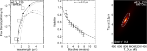
Figure 1: Best fit plots for AFGL230. The first row are figures for the epoch Dec97 and the second row is for Jul02. The first panel in each row shows a fit to the SED with our new photometry included with errors (2MASS points are plotted as squares in each frame for reference). The dashed line represents the contribution from the star, the dotted line represents dust contribution, the dash-dotted line represents the contribution from scattered light, and the solid line is the total flux. The second panel shows our DUSTY fits to the visibility data for each wavelength of observations. The third panel shows the $\chi^{2}/DOF$ surface, with bright areas showing the best-fitting region. The black contour denotes the 1-$\{\sigma\}$ error .

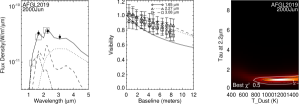
Figure 2: Best fit plots for AFGL2019. See Fig.1 caption.

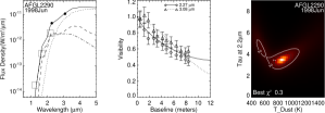
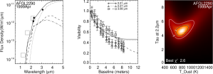
Figure 4: Best fit plots for AFGL2290. See Fig.1 caption.

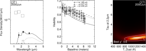
Figure 5: Best fit plots for CIT 1. See Fig.1 caption.

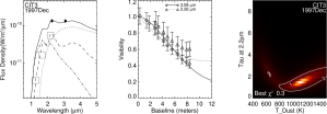
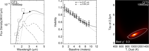
Figure 6: Best fit plots for CIT 3. See Fig.1 caption.

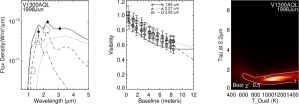
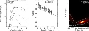
Figure 7: Best fit plots for v1300 Aql. See Fig.1 caption. For the 1999 Jul. epoch we chose the lower-right region as the best fit region because it is consistent with the best fit region for the 1998 Jun. epoch.

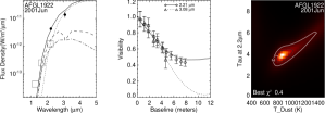
Figure 8: Best fit plots for AFGL1922. See Fig.1 caption.

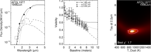
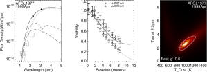
Figure 9: Best fit plots for AFGL1977. See Fig.1 caption.

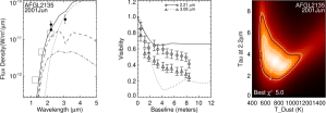
Figure 10: Best fit plots for AFGL2135. See Fig.1 caption.

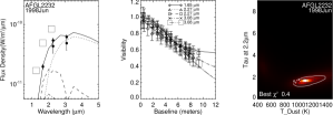
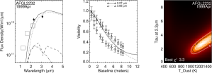
Figure 11: Best fit plots for AFGL2232. See Fig.1 caption.

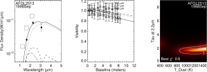
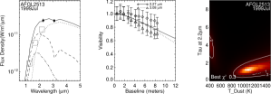
Figure 12: Best fit plots for AFGL2513. See Fig.1 caption.

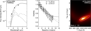
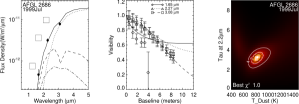
Figure 13: Best fit plots for AFGL2686. See Fig.1 caption.

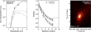
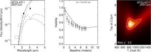
Figure 14: Best fit plots for AFGL4211. See Fig.1 caption.

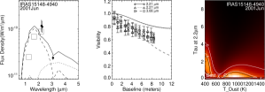
Figure 15: Best fit plots for IRAS15148-4940. See Fig.1 caption. We chose the lower-right region as the best fit region because in all other cases of multiple good fitting regions the one at low tau and high dust temperature was the consistent region.

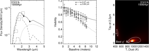
Figure 16: Best fit plots for IY Hya. See Fig.1 caption.

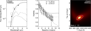
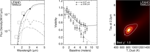
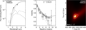
Figure 17: Best fit plots for LP And. See Fig.1 caption.

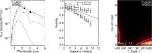
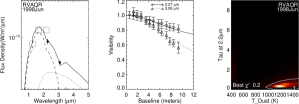
Figure 18: Best fit plots for RV Aqr. See Fig.1 caption.

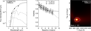
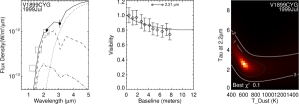
Figure 19: Best fit plots for v1899 Cyg. See Fig.1 caption.

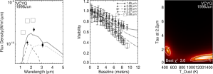
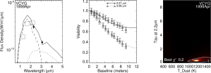
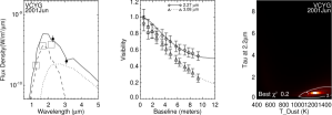
Figure 20: Best fit plots for V Cyg. See Fig.1 caption. For the 1998 Jun. epoch the best fitting region was chosen to be the lower-right region because it is consistent with the other epochs.

In addition to providing the fitting results in tabulated form, we also include here a series of figures which graphically represent the new data, modeling results, and the $\chi^{2}$ surface in our grid. These plots can be found in each of Figures 1–20. The first panel in each figure contains the observed near-IR photometry and best-fit model SED. The second panel in each figure contains the multi-wavelength visibility curves averaged azimuthally along with the model curves. Finally, the third panel shows the $\chi^{2}$ surface in the ($T_{\rm dust}$, $\tau_{2.2\mu\,m}$) plane. We have grouped all the epochs for the same object together so one can see the self-consistency in the derived dust shell parameters – indeed, consistent dust shell properties were recovered when fitting to different epochs, despite large changes in the central star luminosity due to pulsations.

One of the most important results to take away from these panels that we clearly break the standard degeneracy between dust temperature and optical depth. This is because of our new spatial information – by measuring the sizes of the dust shell at various wavelengths we can simultaneously constrain the temperature and optical depth. In the past, one typically had to choose an inner dust temperature based on physical arguments concerning the dust condensation temperatures of various dust species. Here, we see that the inner dust temperature can be constrained independently from other parameters and the implications are discussed further in the next section.

While the simultaneous fits to the near-IR SED and visibility data were generally acceptable, we found the fits to the shortest wavelength visibility data at H band were systematically worse. Since this band is most sensitive to scattering by dust, we explored modified dust distributions, especially using larger grains; we did not find systematic improvements to the fits by altering dust size distribution from MRN or by using other dust constants.

4 Discussion

Our survey provides the first constraints on the asymmetry of the dust shells for such a large sample of dust-enshrouded AGB stars. We found that 4 out of 7 M-stars and 5 of 13 C-stars showed evidence of dust shell asymmetries, with dust shell elongations between 10% and 40%. While this level of asymmetry may sound mild, it actually (quantitatively) compares to the level of asymmetry that would be expected for the most asymmetric dust shells known if placed at 1 kpc. For instance, we know that IRC +10216 (Tuthill et al., 2000a) and CIT 6 (Monnier et al., 2000) have dramatic global asymmetries in their dust shell, detailed imaging made possible by virtue of their proximity. If we placed these targets farther away, we would not be able to image the detail but they would appear $\sim$20% elongated, similar to the degree observed here in 45% of our sample. For CIT 3, we confirm the asymmetries seen by Hofmann et al. (2001) and note that Vinković et al. (2004) showed that the 20% elongation could be explained by a bipolar outflow. That said, clumpy dust formation (Fleischer et al., 1992) might also cause stochastic variations in the inner dust shell geometry that could appear as short-lived elongations. Mid-infrared observations with long-baseline interferometers (e.g, ISI, VLTI-MIDI) should focus on these targets to determine the nature of the asymmetries. In addition, long-term monitoring of these dust shells will help settle debates concerning when the environments of evolved stars develop large scale asymmetries commonly revealed in the later planetary nebula stage. For instance, a long-term asymmetry in a constant position angle (as judged by linear polarization or spatially resolved data) would be a sign of a global bipolar mass-loss asymmetry and not just weather.

In order to look at dust shell properties for our full sample, we have plotted the inner edge dust temperature $T_{\rm dust}$ vs total dust shell optical depth $\tau_{2.2\mu\,m}$ for all our targets. Figure 21 shows these results split into O-rich and C-rich dust type. For K-band optical depths below 2, we find the sublimation temperature of $T_{\rm sub}$(silicates) $=1130\pm 90$ K and $T_{\rm sub}$(amorphous carbon) $=1170\pm 60$ K, both somewhat lower than expected from laboratory measurements (Lodders & Fegley, 1999) and vastly below temperatures inferred from the inner edge of YSO disks ($\sim$1800K, Tannirkulam et al., 2008; Benisty et al., 2010). One component to the observed lower dust temperature could be due to the fact that the central star varies in luminosity by about a factor of 2 during the pulsation cycle and we see the dust cooler than the condensation temperature during phases away from maximum light.

The $T_{\rm dust}$ vs optical depth $\tau_{2.2\mu\,m}$ diagram (Figure 21) also shows no statistically-significant difference between O-rich and C-rich dust types, counter to expectation of higher temperatures for carbon-rich dust (Lodders & Fegley, 1999). We recognise that our simple dust shell modeling may not lead to accurate estimates of the dust sublimation temperature if the inner dust formation environment radically departs from a power law density distribution, perhaps due to pulsations, timescale for dust formation, or multiple dust species. Interestingly though these concerns would likely affect C-rich and O-rich shells similarly and so the lack of a clear difference in sublimation temperatures between these dust types appears robust.

The other important feature of Figure 21, $T_{\rm dust}$ vs optical depth $\tau_{2.2\mu\,m}$, is the apparent temperature at the inner edge of the dust shell gets lower and lower with increasing optical depths above 2. This appears true for both C-rich and O-rich shells. Here we do not believe we are seeing an actual reduction in the dust sublimation temperature, but rather a change in the temperature profile in the inner dust formation zone due to a breakdown in the assumption of a spherically-symmetric $r^{-2}$ density power law. We have ample evidence that dust formation is clumpy, as has been imaged in great detail for IRC +10216 (Tuthill et al., 2000a), but these clumps have been shown to have a relatively weak affect on the temperature structure for low optical depths. Next we further explore how a clumpy dusty environment could change the temperature profile of the dust shell when the individual clumps become themselves optically thick to the stellar and even hot dust radiation field.

Clumpy structures are seen to evolve in 2-D models of dust shells due to self-amplifying density perturbations (e.g. Woitke et al., 2000). First optically thick dust regions form and these regions cast shadows on the dust behind them. Consequently, the temperatures decrease by 100’s of degrees K and this allows for a higher rate of dust formation in these shadow regions. Scattering and re-emission of light by the optical thick regions increases the intensity of radiation between them and eventually the light escapes through the optically thin regions in between the optically thick regions. Thereupon, the temperature within the optically thin regions increases, which decreases the rate of dust production. These processes thus amplify the initial homogeneities until large-scale clumpy structures start to form, such as “dust fingers” (Woitke & Niccolini, 2005). Indeed, Woitke & Niccolini (2005) did see average dust temperatures to be reduced due to these opacity effects but at much weaker level than we see in Figure 21. Realizing that our data reveal a strong effect only at $\tau$’s several times larger than probed by Woitke & Niccolini (2005), we suggest that dust shadowing effects get dramatically stronger when individual clumps become optically thick to both stellar radiation as well as hot dust emission. A 3D radiative transfer calculation of a dusty dust shell could validate or disprove this explanation.

In conclusion, our large sample of spatially resolved dust-enshrouded stars have led to new insights into the late stages of AGB star evolution. We find levels of dust shell elongations that point to significant asymmetries in nearly half of our targets. Our spatial and SED data combined has eliminated some model degeneracies, and we now have the best constraints on the actual sublimation temperatures for dust forming in this outflows, finding lower temperatures than expected from terrestrial experiments and not confirming the large difference expected between carbon-rich and silicate-rich dust. Lastly, we discovered a systematic change in the temperature profile for inner-most dust regions when the dust shell optical depth rises above $\tau_{2.2\mu\,m}>2$. This observed lowering of the central dust temperatures could be naturally explained as a consequence of shadowing caused by clumpy dust formation on spatial scales smaller than our angular resolution, but other possibilities should be further explored as well.

Table 1: Properties of NIRC Camera Infrared Filters. Reference: The NIRC Manual.

Name	Center Wavelength	Bandpass FWHM	Fractional
	$\lambda_{0}$ ( $\mu$m)	$\Delta\lambda$ ( $\mu$m)	Bandwidth
FeII	1.6471	0.0176	1.1%
H	1.6575	0.333	20%
K	2.2135	0.427	19%
Kcont	2.25965	0.0531	2.3%
CH4	2.269	0.155	6.8%
PAHcs	3.0825	0.1007	3.3%

Table 2: Basic Properties of Targets

Source	RA (J2000)	Dec (J2000)	V	Ja	Ha	Ka	Spectral
Names			mag	mag	mag	mag	Type
AFGL 230	01 33 51.21	$+$62 26 53.5	—	16.747	11.232	7.097	M(7)
AFGL 2019	17 53 18.9	$-$26 56 37	20.2(2)	6.338	4.035	2.616	M8(1)
AFGL 2199	18 35 46.48	$+$05 35 46.5	—	8.04	4.85	2.701	M(6)
AFGL 2290	18 58 30.02	$+$06 42 57.7	—	13.169	8.966	5.862	M(6)
CIT 1	00 06 52.94	$+$43 05 00.0	9.00(1)	3.041	1.829	1.115	M9(1)
CIT 3	01 06 25.98	$+$12 35 53.0	—-	7.45	4.641	2.217	M9(1)
v1300 Aql	20 10 27.87	$-$06 16 13.6	20(1)	6.906	3.923	2.059	M(1)
AFGL 1922	17 07 58.24	$-$24 44 31.1	—	12.244	9.181	6.342	C(3)
AFGL 1977	17 31 54.98	$+$17 45 19.7	9.9(4)	10.536	7.994	5.607	C(1)
AFGL 2135	18 22 34.50	$+$27 06 30.2	—	9.043	6.002	3.643	C(1)
AFGL 2232	18 41 54.39	$+$17 41 08.5	9.7(1)	5.742	3.444	1.744	C(1)
AFGL 2513	20 09 14.22	$+$31 25 44.0	—	8.229	5.705	3.69	C(1)
AFGL 2686	20 59 08.88	$+$27 26 41.7	20(1)	9.112	6.268	4.075	Ce(1)
AFGL 4211	15 11 41.89	$-$48 20 01.3	—	10.711	7.751	5.154	C(3)
IRAS 15148-4940	15 18 22.05	$-$49 51 04.6	11.8(1)	5.297	3.071	1.696	C(1)
IY Hya	10 17 00.52	$-$14 39 31.4	14(1)	5.919	3.666	1.964	C(5)
LP And	23 34 27.66	$+$43 33 02.4	—	9.623	6.355	3.859	C(1)
RV Aqr	21 05 51.68	$-$00 12 40.3	11.5(1)	4.046	2.355	1.239	C(5)
v1899 Cyg	21 04 14.8	$+$53 21 03	15.6(1)	10.84	8.693	6.596	C8(5)
V Cyg	20 41 18.2702	$+$48 08 28.835	7.7(1)	3.096	1.273	0.117	C(1)

^a   These magnitudes (from 2MASS) are merely representative since the targets are variable. See Table 3 for our new photometry.
Note: Horizontal line separates oxygen-rich (top) from carbon-rich (bottom).
References: (1) Simbad, (2) Monet (1998), (3) Buscombe (1998), (4) Egret et al. (1992), (5) Skiff (2007), (6) Volk (2002) (7) Garcia-Hernandez et al. (2007)

Table 3: Journal of observations and derived photometry

Target	Date(s)	Filter	Aperture	Magnitude	Calibrator
	(UT)		Mask		Names
AFGL 230	1997 Dec	k	FFA	8.34$\pm$0.1	$\chi$ Cas
		PAHcs	KL Relation*	5.11$\pm$0.2
	2002 Jul	k	FFA	8.99$\pm$0.1	HD 9878
		PAHcs	FFA	5.90$\pm$0.3	HD 9329
AFGL 2019	2000 Jun	CH4	annulus 36	2.48$\pm$0.1	HD 163428
		h	annulus 36	3.84$\pm$ 0.1	HD 156992
		PAHcs	annulus 36	1.52$\pm$0.1	HD 163428
AFGL 2199	1998 Apr	CH4	annulus 36	2.99$\pm$0.1	HD 170137
		PAHcs	annulus 36	1.80$\pm$0.1	HD 170137
AFGL 2290	1998 Jun	CH4	annulus 36	4.72$\pm$0.1	HD 173074
		PAHcs	annulus 36	2.60$\pm$0.1	HD 173074
	1999 Apr	CH4	annulus 36	5.61$\pm$0.1	HD 173833
		k	annulus 36	6.19$\pm$0.32	HD 231437
		PAHcs	annulus 36	3.29$\pm$0.1	HD 173833
CIT 1	2000 Jun	CH4	annulus 36	2.60$\pm$0.1	$\lambda$ And
		h	annulus 36	4.18$\pm$0.25	HD 222499
		PAHcs	annulus 36	1.51$\pm$0.1	$\lambda$ And
CIT 3	1997 Dec	Kcont	annulus 36	1.08$\pm$0.1	$\delta$ Psc
		PAHcs	annulus 36	-0.14$\pm$0.1	$\delta$ Psc
	1998 Sep	CH4	Golay 21	2.45$\pm$0.1	$\delta$ Psc
		PAHcs	Golay 21	1.04$\pm$0.1	$\delta$ Psc
v1300 Aql	1998 Jun	CH4	annulus 36	1.39$\pm$0.1	HD 189114
		h	annulus 36	3.29$\pm$0.25	HD 192464
		PAHcs	annulus 36	0.60$\pm$0.1	HD 189114
	1999 Jul	kcont	annulus 36	2.02$\pm$0.1	SAO 14382
		PAHcs	annulus 36	0.86$\pm$0.1	SAO 14382
AFGL 1922	2000 Jun	k	annulus 36	6.34$\pm$0.25	HD 156992
		PAHcs	KL relation*	3.62$\pm$0.25
	2001 Jun	k	annulus 36	4.90$\pm$0.1	HD 158774
		PAHcs	KL relation*	2.32$\pm$0.25
AFGL 1977	1998 Jun	CH4	annulus 36	4.19$\pm$0.1	HD 158227
		h	annulus 36	7.05$\pm$0.1	HD 158227
		PAHcs	annulus 36	1.84$\pm$0.1	HD 157049
	1999 Apr	CH4	annulus 36	2.77$\pm$0.1	HD 157049
		PAHcs	annulus 36	0.59$\pm$0.1	HD 157049
AFGL 2135	2001 Jun	k	annulus 36	3.29$\pm$0.1	HD 168366, HD 181700
		PAHcs	annulus 36	1.27$\pm$0.3	HD 177716
AFGL 2232	1998 Jun	CH4	annulus 36	2.04$\pm$0.1	HD 158227
		h	annulus 36	4.12$\pm$0.1	HD 158227
		PAHcs	annulus 36	0.68$\pm$0.1	HD 157049
		CH4	Golay 21	2.28$\pm$0.3	HD 168720
		PAHcs	Golay 21	0.94$\pm$0.3	HD 168720
	1999 Apr	CH4	annulus 36	1.06$\pm$0.1	HD 173833
		PAHcs	annulus 36	-0.38$\pm$0.1	HD 173833
AFGL 2513	1998 Sep	h	annulus 36	6.58$\pm$0.1	HD 196241
		CH4	annulus 36	4.03$\pm$0.1	HD 200451
		PAHcs	annulus 36	3.16$\pm$0.3	$\epsilon$ Cyg
	1999 Jul	CH4	annulus 36	2.90$\pm$0.1	HD 188947
		PAHcs	annulus 36	1.70$\pm$0.1	HD 188947
AFGL 2686	1998 Sep	CH4	annulus 36	2.95$\pm$0.1	HD 200451
		h	annulus 36	5.82$\pm$0.21	HD 200451
		PAHcs	annulus 36	1.01$\pm$0.1	$\epsilon$ Cyg, $\lambda$ And
	1999 Jul	CH4	annulus 36	5.13$\pm$0.1	HD 188947
		PAHcs	annulus 36	2.92$\pm$0.1	HD 188947
		h	annulus 36	8.48$\pm$0.3	HD 198330
AFGL 4211	2000 Jun	CH4	annulus 36	3.62$\pm$0.3	HD 137709
		PAHcs	annulus 36	1.42$\pm$0.3	HD 137709
	2001 Jun	k	annulus 36	4.70$\pm$0.1	HD 137709
		PAHcs	KL relation*	2.64$\pm$0.2
IRAS 15148-4940	2001 Jun	CH4	annulus 36	1.25$\pm$0.3	HD 137709
		k	annulus 36	1.30$\pm$0.3	HD 137709
		PAHcs	annulus 36	1.71$\pm$0.1	HD 136422
IY Hya	1999 Apr	CH4	annulus 36	2.08$\pm$0.1	HD 87262
		PAHcs	annulus 36	1.37$\pm$0.1	$\mu$ Hya
LP And	1998 Sep	CH4	annulus 36	3.89$\pm$0.1	HD 222499, $\lambda$ And
		h	annulus 36	7.05$\pm$0.25	HD 222499
		PAHcs	annulus 36	1.72$\pm$0.1	$\lambda$ And
	1999 Jul	CH4	Golay 21	4.01$\pm$0.1	$\alpha$ Cas
		PAHcs	Golay 21	1.80$\pm$0.1	$\alpha$ Cas
	1999 Jan	CH4	Golay 21	3.26$\pm$0.1	$\alpha$ Cas
		PAHcs	Golay 21	1.18$\pm$0.1	$\alpha$ Cas
RV Aqr	1999 Jul	CH4	Golay 21	1.23$\pm$0.25	SAO 143482, 3 Aqr
		PAHcs	Golay 21	0.56$\pm$0.25	SAO 143482, 3 Aqr
	1998 Jun	CH4	Golay 21	1.52$\pm$0.1	HD 196321
		PAHcs	Golay 21	1.15$\pm$0.1	HD 196321
v1899 Cyg	1998 Jun	CH4	annulus 36	5.53$\pm$0.1	HD 202897
		h	annulus 36	7.87$\pm$0.3	HD 200817
		PAHcs	annulus 36	3.71$\pm$0.1	HD 202897
	1999 Jul	k	annulus 36	6.40$\pm$0.1	HD 198661
		PAHcs	KL relation*	4.72$\pm$0.2
V Cyg	1998 Jun	feii	annulus 36	2.59$\pm$0.1	HD 192909
		kcont	annulus 36	0.53$\pm$0.1	HD 192909
		CH4	Golay 21	0.50$\pm$0.1	HD 192909
		PAHcs	annulus 36	0.26$\pm$0.1	HD 192909
		PAHcs	Golay 21	0.19$\pm$0.1	HD 192909
	1999 Apr	CH4	Golay 21	0.15$\pm$0.1	$\xi$ Cyg
		PAHcs	Golay 21	-0.25$\pm$0.1	$\xi$ Cyg
	2001 Jun	CH4	annulus 36	-0.27$\pm$0.1	$\xi$ Cyg
		PAHcs	annulus 36	-0.69$\pm$0.1	$\xi$ Cyg

*   This point was extrapolated from another epoch for the same star and assigned an error of 0.2 mag.
Note: Horizontal line separates oxygen-rich (top) from carbon-rich (bottom).

Table 4: Basic Properties of Calibrators

Calibrator	J	H	K	PAHcs	Reference
	mag	mag	mag	mag
HD 168720	1.79	0.875	0.870	0.794	McWilliam & Lambert (1984), Cutri (2003), Neugebauer & Leighton (1969)
HD 170137	3.476	2.737	2.230	2.16	Cutri (2003), Neugebauer & Leighton (1969)
$\epsilon$ Cyg	0.641	0.2	0.1	0.011	Neugebauer & Leighton (1969), Ghosh et al. (1984), Price & Murdock (1999)
HD 200451	4.101	3.231	2.840	—	Cutri (2003), Neugebauer & Leighton (1969)
HD 231437	5.027	3.958	3.693	—	Cutri (2003)
HD 173833	3.488	2.647	2.1	2.02	Cutri (2003), Neugebauer & Leighton (1969)
HD 158227	5.626	4.984	4.812	—	Cutri (2003)
HD 157049	1.975	1.149	.830	.684	Cutri (2003), Neugebauer & Leighton (1969), Price & Murdock (1999)
HD 168366	5.049	4.535	4.255	—	Cutri (2003)
HD 181700	3.938	2.993	2.735	—	Cutri (2003)
SAO 143482	1.665	0.790	0.573	0.436	Cutri (2003), Gullixson et al. (1983)
HD 189114	3.212	2.030	1.953	1.908	Cutri (2003), Gosnell et al. (1979)
HD 137709	2.232	1.532	1.331	1.257	Cutri (2003), extrapolation
HD 222499	4.641	3.804	3.627	—	Cutri (2003)
$\lambda$ And	1.970	1.4	1.287	1.245	Johnson et al. (1966), Price & Murdock (1999), Selby et al. (1988)
HD 9878	6.631	6.730	6.698	—	Cutri (2003)
HD 9329	4.961	4.381	4.341	4.29	Cutri (2003), extrapolation
HD 156992	3.901	3.123	2.926	—	Cutri (2003)
HD 158774	4.403	3.451	3.138	—	Cutri (2003), Kawara et al. (1983)
HD 198611	3.755	2.862	2.470	—	Cutri (2003), Cutri (2003), Neugebauer & Leighton (1969)
HD 202987	3.859	3.067	2.82	2.75	Cutri (2003), Neugebauer & Leighton (1969)
3 Aqr	0.934	-0.020	-0.220	-0.338	Carter (1990)
HD 192909	1.190	—	0.180	0.101	Johnson et al. (1966), Neugebauer & Leighton (1969), Price & Murdock (1999)
$\xi$ Cyg	.995	0.130	-0.070	-0.150	Johnson et al. (1966), Noguchi et al. (1981)
HD 200817	4.174	3.721	3.708	—	Cutri (2003)
HD 192464	5.180	4.176	3.879	—	Cutri (2003)
$\alpha$ Cas	0.371	-0.191	-0.270	-0.399	Voelcker (1975), Alonso et al. (1994)
$\mu$ Hya	1.216	.506	0.37	0.28	Cutri (2003), Price & Murdock (1999), Johnson et al. (1966)
HD 87262	2.974	2.052	1.880	—	Cutri (2003), Price & Murdock (1999), Neugebauer & Leighton (1969)
HD 196321	2.128	1.361	1.21	.98496	Cutri (2003), Price & Murdock (1999), Neugebauer & Leighton (1969)
HD 136422	—	—	0.8	0.535	Price (1968), Price & Murdock (1999), Eggen (1969)
$\delta$ Psc	2.031	1.198	.890	0.739	Cutri (2003), Gosnell et al. (1979)
HD 198330	4.988	4.159	3.816	—	Cutri (2003)
HD 188947	1.934	1.438	1.621	1.561	Noguchi et al. (1981), Elias et al. (1982), Glass (1975)
$\chi$ Cas	3.019	2.481	2.311	—	Cutri (2003), Neugebauer & Leighton (1969)
HD 163428	—	—	1.6	1.464	White & Wing (1978), Humphreys & Ney (1974)
HD 196241	4.19	3.620	3.090	—	Morel & Magnenat (1978), Cutri (2003)

Table 5: Results from Circularly-Symmetric Gaussian Models

Target	Date(s)	Filter	Aperture	$V_{0}$	FWHM	$\chi$2/DOF
				($\pm$0.05)	(mas)
AFGL 230	1997 Dec	k	FFA	0.71	32$\pm$3	0.23
	2002 Jul	k	FFA	0.54	34$\pm$3	0.34
		PAHcs	FFA	0.74	33$\pm$2	0.05
AFGL 2019	2000 Jun	CH4	annulus 36	0.96	10${}^{+6}_{-10}$	0.31
		h	annulus 36	0.90	9$\pm$4	0.65
		PAHcs	annulus 36	0.95	21$\pm$3	0.27
AFGL 2199	1998 Apr	CH4	annulus 36	0.92	14$\pm$6	0.23
		PAHcs	annulus 36	1.00	22$\pm$3	0.45
AFGL 2290*	1998 Jun	CH4	annulus 36	0.76	22$\pm$4	0.33
		PAHcs	annulus 36	0.84	27$\pm$3	0.69
	1999 Apr	CH4	annulus 36	0.72	34$\pm$3	0.39
		k	annulus 36	0.75	32$\pm$3	0.51
		PAHcs	annulus 36	0.83	36$\pm$2	0.36
Cit 1*	2000 Jun	CH4	annulus 36	0.92	15$\pm$5	0.35
		h	annulus 36	0.93	14$\pm$3	0.37
		PAHcs	annulus 36	0.94	20$\pm$4	0.46
Cit 3*	1997 Dec	kcont	annulus 36	0.89	20$\pm$5	0.44
		PAHcs	annulus 36	0.89	37$\pm$2	0.21
	1998 Sep	CH4	Golay 21	0.89	21$\pm$4	0.35
		PAHcs	Golay 21	0.90	29$\pm$2	0.25
v1300 Aql*	1998 Jun	CH4	annulus 36	0.83	14$\pm$6	0.43
		h	annulus 36	0.81	14$\pm$3	0.41
		PAHcs	annulus 36	0.84	23$\pm$3	0.50
	1999 Jul	kcont	annulus 36	0.87	18$\pm$5	0.39
		PAHcs	annulus 36	0.90	21$\pm$3	0.52
AFGL 1922	2000 Jun	k	annulus 36	0.76	24$\pm$4	0.88
	2001 Jun	k	annulus 36	0.83	29$\pm$4	0.76
		PAHcs	annulus 36	0.95	58$\pm$2	0.43
AFGL 1977*	1998 Jun	CH4	annulus 36	0.78	24$\pm$4	0.26
		h	annulus 36	0.76	17$\pm$3	0.68
		PAHcs	annulus 36	0.94	34$\pm$2	0.41
	1999 Apr	CH4	annulus 36	0.96	29$\pm$4	0.25
		PAHcs	annulus 36	0.89	52$\pm$2	0.26
AFGL 2135	2001 Jun	k	annulus 36	0.66	17$\pm$5	0.49
	2001 Jun	PAHcs	annulus 36	0.50	34$\pm$2	0.13
AFGL 2232*	1998 Jun	CH4	annulus 36	0.83	18$\pm$5	1.32
		h	annulus 36	0.81	14$\pm$3	0.50
		PAHcs	annulus 36	0.90	33$\pm$2	0.56
		CH4	Golay 21	0.91	20$\pm$5	0.17
		PAHcs	Golay 21	0.90	34$\pm$2	0.14
	1999 Apr	CH4	annulus 36	0.69	44$\pm$3	0.19
		PAHcs	annulus 36	0.86	42$\pm$2	0.12
AFGL 2513*	1998 Sep	h	annulus 36	1.00	1${}^{+9}_{-1}$	1.15
		CH4	annulus 36	0.94	10${}^{+6}_{-10}$	0.18
		PAHcs	annulus 36	1.00	16$\pm$4	0.70
	1999 Jul	CH4	annulus 36	1.00	11${}^{+6}_{-9}$	0.32
		PAHcs	annulus 36	0.96	24$\pm$3	0.36
AFGL 2686	1998 Sep	CH4	annulus 36	0.89	29$\pm$4	0.44
		h	annulus 36	0.89	26$\pm$2	0.47
		PAHcs	annulus 36	0.89	35$\pm$2	0.36
	1999 Jul	CH4	annulus 36	0.92	26$\pm$4	0.68
		PAHcs	annulus 36	0.91	33$\pm$2	0.44
		h	annulus 36	0.77	28$\pm$2	0.87
AFGL 4211	2000 Jun	CH4	annulus 36	0.78	31$\pm$3	0.48
		PAHcs	annulus 36	0.82	70$\pm$3	0.10
	2001 Jun	k	annulus 36	0.62	20$\pm$5	0.63
IRAS 15148-4940	2001 Jun	CH4	annulus 36	0.77	13$\pm$7	0.41
		k	annulus 36	0.82	13$\pm$7	0.59
		PAHcs	annulus 36	0.86	25$\pm$3	0.39
IY Hya	1999 Apr	CH4	annulus 36	0.88	14$\pm$6	0.32
		PAHcs	annulus 36	0.94	33$\pm$2	0.28
LP And*	1998 Sep	CH4	annulus 36	0.83	25$\pm$4	0.52
		h	annulus 36	0.68	20$\pm$3	0.56
		PAHcs	annulus 36	0.86	47$\pm$2	0.49
	1999 Jul	CH4	Golay 21	0.89	24$\pm$4	0.99
		PAHcs	Golay 21	0.79	48$\pm$2	0.50
	1999 Jan	CH4	Golay 21	0.70	25$\pm$4	2.41
		PAHcs	Golay 21	0.66	35$\pm$2	0.45
RV Aqr*	1999 Jul	CH4	Golay 21	1.00	8$\pm$8	0.16
		PAHcs	Golay 21	0.96	26$\pm$3	0.21
	1998 Jun	CH4	Golay 21	0.98	12$\pm$8	0.13
		PAHcs	Golay 21	1.00	27$\pm$3	0.36
v1899 Cyg	1998 Jun	CH4	annulus 36	0.88	18$\pm$5	0.35
		h	annulus 36	0.86	16$\pm$3	0.39
		PAHcs	annulus 36	0.92	22$\pm$3	0.32
	1999 Jul	k	annulus 36	0.93	15$\pm$5	0.62
V Cyg	1998 Jun	feii	annulus 36	0.87	14$\pm$3	0.92
		kcont	annulus 36	0.96	16$\pm$5	1.15
		PAHcs	annulus 36	0.90	34$\pm$2	0.51
		CH4	Golay 21	1.00	18$\pm$5	0.35
		PAHcs	Golay 21	0.92	38$\pm$2	0.10
	1999 Apr	CH4	Golay 21	0.93	17$\pm$5	0.15
		PAHcs	Golay 21	0.86	38$\pm$2	0.12
	2001 Jun	CH4	annulus 36	0.82	19$\pm$5	0.26
		PAHcs	annulus 36	0.83	42$\pm$2	0.15

*   target is asymmetric, see Table 7 for further details
Note: Horizontal line separates oxygen-rich (top) from carbon-rich (bottom).

Table 6: Results from Central Point plus Circularly-Symmetric Gaussian Models

Target	Date(s)	Filter	Aperture	fPoint	fGauss	FWHM	$\chi^{2}$/DOF
				($\pm$.05)	($\pm$0.05)	(mas)
AFGL 230	1997 Dec	k	FFA	0.24	0.52	47$\pm$7	0.21
	2002 Jul	k	FFA	0.30	0.42	98$\pm$7	0.15
		PAHcs	FFA	0.50	0.32	86$\pm$8	0.42
AFGL 2019	2000 Jun	CH4	annulus 36	0.86	0.14	51${}^{+30}_{-45}$	0.28
		h	annulus 36	0.00	0.83	1${}^{+9}_{-1}$	0.83
		PAHcs	annulus 36	0.45	0.51	31$\pm$5	0.27
AFGL 2199	1998 Apr	CH4	annulus 36	0.38	0.54	19$\pm$9	0.22
		PAHcs	annulus 36	0.36	0.68	30$\pm$4	0.43
AFGL 2290*	1998 Jun	CH4	annulus 36	0.44	0.38	46$\pm$12	0.26
		PAHcs	annulus 36	0.55	0.38	68$\pm$7	0.61
	1999 Apr	CH4	annulus 36	0.31	0.51	66$\pm$9	0.21
		k	annulus 36	0.34	0.56	66$\pm$9	0.31
		PAHcs	annulus 36	0.25	0.60	49$\pm$3	0.35
CIT 1*	2000 Jun	CH4	annulus 36	0.00	0.92	14$\pm$6	0.35
		h	annulus 36	0.47	0.49	23$\pm$6	0.36
		PAHcs	annulus 36	0.00	0.94	20$\pm$4	0.46
CIT 3 *	1997 Dec	kcont	annulus 36	0.58	0.50	53$\pm$13	0.23
		PAHcs	annulus 36	0.36	0.62	60$\pm$4	0.02
	1998 Sep	CH4	Golay 21	0.50	0.44	40$\pm$10	0.03
		PAHcs	Golay 21	0.46	0.47	50$\pm$5	0.20
v1300 Aql*	1998 Jun	CH4	annulus 36	0.64	0.23	43$\pm$20	0.40
		h	annulus 36	0.45	0.38	25$\pm$7	0.39
		PAHcs	annulus 36	0.64	0.34	80$\pm$10	0.30
	1999 Jul	kcont	annulus 36	0.00	0.87	18$\pm$5	0.39
		PAHcs	annulus 36	0.17	0.73	24$\pm$4	0.52
AFGL 1922	2000 Jun	k	annulus 36	0.42	0.39	47$\pm$11	0.83
	2001 Jun	k	annulus 36	0.43	0.49	57$\pm$12	0.62
		PAHcs	annulus 36	0.51	0.47	105$\pm$6	0.41
AFGL 1977*	1998 Jun	CH4	annulus 36	0.36	0.45	41$\pm$9	0.22
		h	annulus 36	0.50	0.33	43${}^{+8}_{-13}$	0.59
		PAHcs	annulus 36	0.42	0.58	56$\pm$4	0.36
	1999 Apr	CH4	annulus 36	0.34	0.69	43$\pm$7	0.17
		PAHcs	annulus 36	0.25	0.74	45$\pm$3	0.17
AFGL 2135	2001 Jun	k	annulus 36	0.00	0.66	17$\pm$5	0.49
	2001 Jun	PAHcs	annulus 36	0.28	0.27	78$\pm$6	0.10
AFGL 2232*	1998 Jun	CH4	annulus 36	0.56	0.33	44$\pm$14	0.47
		h	annulus 36	0.00	0.81	14$\pm$3	1.32
		PAHcs	annulus 36	0.50	0.49	66$\pm$6	0.49
		CH4	Golay 21	0.52	0.45	39$\pm$10	0.10
		PAHcs	Golay 21	0.35	0.60	51$\pm$4	0.09
	1999 Apr	CH4	annulus 36	0.23	0.56	72$\pm$7	0.08
		PAHcs	annulus 36	0.26	0.64	58$\pm$3	0.07
AFGL 2513*	1998 Sep	h	annulus 36	0.03	1.00	1${}^{+9}_{-1}$	1.09
		CH4	annulus 36	0.81	0.14	39$\pm$39	0.17
		PAHcs	annulus 36	0.03	1.00	19$\pm$4	0.68
	1999 Jul	CH4	annulus 36	0.00	0.92	1${}^{+13}_{-1}$	0.65
		PAHcs	annulus 36	0.67	0.37	65$\pm$9	0.24
AFGL 2686	1998 Sep	CH4	annulus 36	0.30	0.63	42$\pm$7	0.39
		h	annulus 36	0.24	0.69	35$\pm$4	0.43
		PAHcs	annulus 36	0.39	0.56	58$\pm$4	0.29
	1999 Jul	CH4	annulus 36	0.21	0.73	32$\pm$5	0.67
		PAHcs	annulus 36	0.29	0.64	45$\pm$3	0.42
		h	annulus 36	0.63	0.30	138${}^{+15}_{-9}$	0.77
AFGL 4211	2000 Jun	CH4	annulus 36	0.36	0.54	59$\pm$10	0.27
		PAHcs	annulus 36	0.16	0.70	89$\pm$4	0.06
	2001 Jun	k	annulus 36	0.47	0.28	86${}^{+9}_{-19}$	0.45
IRAS 15148-4940	2001 Jun	CH4	annulus 36	0.62	0.18	44$\pm$23	0.39
		k	annulus 36	0.52	0.31	25$\pm$13	0.59
		PAHcs	annulus 36	0.52	0.38	49$\pm$7	0.37
IY Hya	1999 Apr	CH4	annulus 36	0.00	0.88	14$\pm$6	0.32
		PAHcs	annulus 36	0.00	0.94	32$\pm$2	0.28
LP And*	1998 Sep	CH4	annulus 36	0.42	0.49	49$\pm$10	0.41
		h	annulus 36	0.37	0.34	39$\pm$9	0.52
		PAHcs	annulus 36	0.30	0.65	74$\pm$4	0.35
	1999 Jul	CH4	Golay 21	0.47	0.49	47$\pm$11	0.91
		PAHcs	Golay 21	0.35	0.51	85$\pm$5	0.42
	1999 Jan	CH4	Golay 21	0.47	0.49	47$\pm$11	0.91
		PAHcs	Golay 21	0.35	0.51	85$\pm$5	0.42
RV Aqr*	1999 Jul	CH4	Golay 21	0.00	0.96	1${}^{+13}_{-1}$	0.30
		PAHcs	Golay 21	0.33	0.64	34$\pm$4	0.21
	1998 Jun	CH4	Golay 21	0.74	0.25	30$\pm$20	0.12
		PAHcs	Golay 21	0.43	0.62	42$\pm$4	0.33
v1899 Cyg	1998 Jun	CH4	annulus 36	0.32	0.57	24$\pm$7	0.35
		h	annulus 36	0.72	0.23	75$\pm$15	0.30
		PAHcs	annulus 36	0.65	0.23	57$\pm$13	0.31
	1999 Jul	k	annulus 36	0.76	0.23	52$\pm$24	0.59
V Cyg	1998 Jun	feii	annulus 36	0.31	0.56	18$\pm$5	0.91
		kcont	annulus 36	0.51	0.47	26$\pm$9	1.14
		PAHcs	annulus 36	0.00	0.90	34$\pm$2	0.51
		CH4	Golay 21	0.58	0.47	35$\pm$10	0.30
		PAHcs	Golay 21	0.28	0.67	52$\pm$3	0.06
	1999 Apr	CH4	Golay 21	0.52	0.43	30$\pm$9	0.14
		PAHcs	Golay 21	0.31	0.60	57$\pm$4	0.07
	2001 Jun	CH4	annulus 36	0.50	0.36	40$\pm$11	0.21
		PAHcs	annulus 36	0.28	0.61	63$\pm$4	0.09

*   target is asymmetric, see Table 7 for further details

Note: Horizontal line separates oxygen-rich (top) from carbon-rich (bottom).

Table 7: Results from 2-dimensional Gaussian Models

Target	Date(s)	Filter	$\frac{{\rm FWHM}_{\rm major}}{{\rm FWHM}_{\rm minor}}$	$<$PA$>$
AFGL 2290	1998 Jun	CH4	1.23	58$\pm$20
		PAHcs	1.24
	1999 Apr	CH4	1.24
		k	1.24
		PAHcs	1.06
CIT 1	2000 Jun	CH4	1.13	133$\pm$3
		h	1.14
		PAHcs	1.11
CIT 3	1997 Dec	Kcont	1.19	151$\pm$9
		PAHcs	1.06
	1998 Sep	CH4	1.28
		PAHcs	1.04
v1300 Aql	1998 Jun	CH4	1.34	108$\pm$13
		h	1.14
		PAHcs	1.19
	1999 Jul	kcont	1.34
		PAHcs	1.31
AFGL 1977	1998 Jun	CH4	1.11	71$\pm$18
		h	1.31
		PAHcs	1.06
	1999 Apr	CH4	1.10
		PAHcs	1.21
AFGL 2232	1998 Jun	CH4	1.37	94$\pm$10
		h	1.83
		PAHcs	1.19
		CH4	1.10
		PAHcs	1.08
	1999 Apr	CH4	1.22
		PAHcs	1.05
AFGL 2513	1998 Sep	h	unresolved
		CH4	1.5	61$\pm$8
		PAHcs	1.39
	1999 Jul	CH4	1.38
		PAHcs	1.2
LP And	1998 Sep	CH4	1.46	108$\pm$6
		h	2.03
		PAHcs	1.39
	1999 Jul	CH4	1.64
		PAHcs	1.36
	1999 Jan	CH4	1.82
		PAHcs	1.20
RV Aqr	1999 Jul	CH4	1.49	122$\pm$24
		PAHcs	1.23
	1998 Jun	CH4	1.35
		PAHcs	1.22

* Sources missing from this list were found to have circularly-symmetric dust shells (within errors). Note: PA is the mean position angle of the major axis (degrees East of North) for all filters and epochs.

Table 8: Results from DUSTY Radiative Transfer Model

Target	Date(s)	Tdust	$\tau_{2.2\mu\,m}$	R∗	L${}_{\ast}^{(1\,kpc)}$	$\chi^{2}$/DOF
		(K)		(mas)	$(10^{3}$ L⊙)
AFGL 230	1997 Dec	800${}^{+60}_{-90}$	4.9${}^{+0.9}_{-0.7}$	1.5${}^{+0.5}_{-0.3}$	4.5${}^{+3.1}_{-1.6}$	0.26
	2002 Jul	540${}^{+400}_{-110}$	7.4${}^{+1.6}_{-1.2}$	4.1${}^{+4.5}_{-2.1}$	31${}^{+108}_{-24}$	3.86
AFGL 2019	2000 Jun	1190${}^{+310}_{-250}$	0.92${}^{+0.23}_{-0.12}$	3.5${}^{+0.7}_{-0.3}$	24${}^{+10}_{-4}$	0.54
AFGL 2199	1998 Apr	1130${}^{+370}_{-310}$	1.6${}^{+1.2}_{-0.7}$	3.3${}^{+2.0}_{-0.6}$	21${}^{+32}_{-7}$	0.06
AFGL 2290	1998 Jun	850${}^{+140}_{-80}$	3.5${}^{+0.5}_{-0.5}$	3.7${}^{+0.8}_{-0.7}$	26${}^{+12}_{-9}$	0.33
	1999 Apr	800${}^{+140}_{-140}$	4.6${}^{+0.7}_{-0.5}$	3.9${}^{+1.7}_{-0.8}$	29${}^{+31}_{-11}$	2.63
CIT 1	2000 Jun	1190${}^{+310}_{-230}$	1.2${}^{+0.5}_{-0.2}$	3.5${}^{+0.8}_{-0.4}$	24${}^{+12}_{-5}$	0.60
CIT 3	1997 Dec	1110${}^{+230}_{-140}$	1.4${}^{+0.7}_{-0.5}$	7.8${}^{+1.5}_{-0.6}$	116${}^{+49}_{-16}$	0.34
	1998 Sep	1020${}^{+200}_{-110}$	1.9${}^{+0.7}_{-0.5}$	5.0${}^{+0.8}_{-0.6}$	48${}^{+17}_{-11}$	0.29
v1300 Aql	1998 Jun	1080${}^{+340}_{-170}$	0.92${}^{+0.46}_{-0.12}$	5.8${}^{+1.0}_{-0.6}$	64${}^{+24}_{-12}$	0.50
	1999 Jul	1160${}^{+340}_{-250}$*	1.60${}^{+0.9}_{-0.7}$*	5.1${}^{+2.0}_{-0.8}$	49${}^{+45}_{-14}$	0.11
AFGL 1922	2000 Jun	850${}^{+200}_{-60}$	5.3${}^{+0.7}_{-0.7}$	4.5${}^{+1.1}_{-0.8}$	37${}^{+21}_{-13}$	1.44
	2001 Jun	850${}^{+170}_{-60}$	3.9${}^{+0.5}_{-0.5}$	5.2${}^{+1.2}_{-1.5}$	51${}^{+27}_{-25}$	0.39
AFGL 1977	1998 Jun	910${}^{+80}_{-90}$	2.8${}^{+0.1}_{-0.2}$	4.0${}^{+0.2}_{-0.6}$	31${}^{+4}_{-8}$	1.69
	1999 Apr	990${}^{+90}_{-60}$	2.5${}^{+0.5}_{-0.2}$	6.0${}^{+0.8}_{-0.4}$	68${}^{+19}_{-9}$	0.65
AFGL 2135	2001 Jun	740${}^{+370}_{-200}$	3.2${}^{+4.2}_{-1.4}$	9.4${}^{+65.7}_{-4.6}$	167${}^{+10500}_{-123}$	5.04
AFGL 2232	1998 Jun	1110${}^{+140}_{-110}$	1.6${}^{+0.2}_{-0.2}$	5.1${}^{+0.5}_{-0.5}$	48${}^{+11}_{-10}$	0.32
	1999 Apr	1300${}^{+200}_{-230}$	2.8${}^{+1.4}_{-1.2}$	9.4${}^{+5.0}_{-1.2}$	165${}^{+226}_{-41}$	3.29
AFGL 2513	1998 Sep	1500${}^{+0}_{-450}$	1.9${}^{+0.2}_{-0.2}$	1.7${}^{+0.9}_{-0.2}$	5.3${}^{+7.3}_{-0.9}$	0.57
	1999 Jul	1110${}^{+400}_{-200}$	1.2${}^{+0.9}_{-0.5}$	3.1${}^{+1.0}_{-0.4}$	18${}^{+14}_{-4}$	0.30
AFGL 2686	1998 Sep	1110${}^{+140}_{-140}$	2.8${}^{+0.5}_{-0.5}$	5.3${}^{+1.1}_{-0.8}$	53${}^{+24}_{-15}$	1.85
	1999 Jul	820${}^{+60}_{-60}$	3.2${}^{+0.2}_{-0.2}$	3.1${}^{+0.4}_{-0.3}$	19${}^{+4}_{-4}$	1.02
AFGL 4211	2000 Jun	880${}^{+60}_{-30}$	3.7${}^{+0.7}_{-0.5}$	6.7${}^{+0.3}_{-0.3}$	85${}^{+9}_{-7}$	0.73
	2001 Jun	850${}^{+170}_{-80}$	4.2${}^{+0.9}_{-0.7}$	6.1${}^{+3.7}_{-2.0}$	71${}^{+113}_{-39}$	3.20
IRAS 15148-4940	2001 Jun	940${}^{+340}_{-170}$*	0.23${}^{+0.46}_{-0.12}$	4.6${}^{+0.2}_{-0.9}$	40${}^{+4}_{-14}$	2.47
IY Hya	1999 Apr	960${}^{+140}_{-110}$	0.46${}^{+0.46}_{-0.12}$	4.2${}^{+0.1}_{-0.2}$	33${}^{+2}_{-3}$	0.25
LP And	1998 Sep	880${}^{+70}_{-60}$	3.0${}^{+0.5}_{-0.2}$	4.8${}^{+0.9}_{-0.5}$	43${}^{+19}_{-8}$	1.49
	1999 Jul	820${}^{+60}_{-60}$	3.0${}^{+0.2}_{-0.5}$	4.8${}^{+0.6}_{-0.7}$	44${}^{+12}_{-12}$	1.00
	1999 Jan	880${}^{+90}_{-30}$	3.2${}^{+0.5}_{-0.2}$	6.7${}^{+1.0}_{-0.7}$	85${}^{+27}_{-17}$	1.67
RV Aqr	1999 Jul	1500${}^{+0}_{-280}$	0.46${}^{+0.23}_{-0.23}$	5.4${}^{+0.7}_{-0.4}$	55${}^{+15}_{-7}$	1.09
	1998 Jun	1190${}^{+310}_{-150}$	0.23${}^{+0.46}_{-0.12}$	5.1${}^{+0.1}_{-0.7}$	48${}^{+2}_{-13}$	0.23
v1899 Cyg	1998 Jun	740${}^{+60}_{-60}$	2.3${}^{+0.5}_{-0.2}$	2.0${}^{+0.5}_{-0.3}$	7.5${}^{+3.8}_{-1.8}$	0.53
	1999 Jul	600${}^{+340}_{-200}$	2.5${}^{+2.5}_{-1.2}$	1.8${}^{+4.4}_{-1.0}$	6.1${}^{+66}_{-4.8}$	0.12
V Cyg	1998 Jun	1270${}^{+230}_{-200}$*	0.69${}^{+0.46}_{-0.23}$*	6.6${}^{+0.7}_{-0.1}$	83${}^{+19}_{-3}$	3.02
	1999 Apr	1160${}^{+200}_{-110}$	0.23${}^{+0.23}_{-0.12}$	9.6${}^{+0.3}_{-1.2}$	174${}^{+11}_{-40}$	0.21
	2001 Jun	1270${}^{+140}_{-140}$	0.46${}^{+0.23}_{-0.23}$	10.6${}^{+1.6}_{-0.6}$	212${}^{+70}_{-24}$	0.24

*   This star has two regions which meet our 1-$\sigma$ criteria for a best fit. The particular values shown were chosen for consistency, see the appropriate figure for more details.
Note: Horizontal line separates oxygen-rich (top) from carbon-rich (bottom).

Figure 3: Best fit plots for AFGL2199. See Fig.1 caption.

Figure 21: A plot of best fit $\tau_{2.2\mu\,m}$ versus the temperature at the inner edge of dust shell T_dust. Open symbols are used for oxygen-rich dust shells and closed symbols are used for carbon-rich dust shells.

References

- Alonso et al. (1994) Alonso, A., Arribas, S., & Martinez-Roger, C. 1994, Astronomy and Astrophysics, 282, 684
- Balick & Frank (2002) Balick, B. & Frank, A. 2002, Annual Review of Astronomy and Astrophysics, 40, 439
- Benisty et al. (2010) Benisty, M., Natta, A., Isella, A., Berger, J.-P., Massi, F., Le Bouquin, J.-B., Mérand, A., Duvert, G., Kraus, S., Malbet, F., Olofsson, J., Robbe-Dubois, S., Testi, L., Vannier, M., & Weigelt, G. 2010, Astronomy and Astrophysics, 511, A74
- Buscombe (1998) Buscombe, W. 1998, Vizier On-line Data Catalog: III/206
- Carter (1990) Carter, B. S. 1990, Royal Astronomical Society, Monthly Notices, 242, 1
- Cutri (2003) Cutri, R. M. e. a. 2003, The IRSA 2MASS All-Sky Point Source Catalog, NASA/IPAC Infrared Science Archive
- Danchi et al. (1994) Danchi, W. C., Bester, M., Degiacomi, C. G., Greenhill, L. J., & Townes, C. H. 1994, Astronomical Journal, 107, 1469
- Danchi et al. (2001) Danchi, W. C., Tuthill, P. G., & Monnier, J. D. 2001, Astrophysical Journal, 562, 440
- Eggen (1969) Eggen, O. J. 1969, Astrophysical Journal, 158, 225
- Egret et al. (1992) Egret, D., Didelon, P., Mclean, B. J., Russell, J. L., & Turon, C. 1992, AA, 258, 217
- Elias et al. (1982) Elias, J. H., Frogel, J. A., Matthews, K., & Neugebauer, G. 1982, Astronomical Journal, 87, 1029
- Fleischer et al. (1992) Fleischer, A. J., Gauger, A., & Sedlmayr, E. 1992, Astronomy and Astrophysics, 266, 321
- Garcia-Hernandez et al. (2007) Garcia-Hernandez, D., Garcia-Lario, P., Plez, B., Manchado, A., D’Antona, F., Lub, J., & Habing, H. 2007, Astronomy and Astrophysics, 462, 711
- Gezari et al. (1999) Gezari, D. Y., Pitts, P. S., & Schmitz, M. 1999, VizieR Online Data Catalog, 2225, 0
- Ghosh et al. (1984) Ghosh, S., Iyengar, K. V. K., Tandon, S. N., Verma, R. P., Daniel, R. R., & Rengarajan, T. N. 1984, Royal Astronomical Society, Monthly Notices, 206, 611
- Glass (1975) Glass, I. S. 1975, Mon. Not. R. Astron. Soc., 171, 19P
- Gosnell et al. (1979) Gosnell, T. R., Hudson, H., & Peutter, R. C. 1979, Astronomical Journal, 84, 538
- Gullixson et al. (1983) Gullixson, C., Gehrz, R. D., Hackwell, J. A., Grasdalen, G. L., & Castelaz, M. 1983, Astrophysical Journal Supplement Series, 53, 413
- Haniff & Buscher (1998) Haniff, C. A. & Buscher, D. F. 1998, Astronomy and Astrophysics, 334, L5
- Hanner (1988) Hanner, M. 1988, Grain optical properties, Tech. rep.
- Hauschildt et al. (1999) Hauschildt, P. H., Allard, F., Ferguson, J., Baron, E., & Alexander, D. R. 1999, Astrophysical Journal, 525, 871
- Hofmann et al. (2001) Hofmann, K.-H., Balega, Y., Blöcker, T., & Weigelt, G. 2001, Astronomy and Astrophysics, 379, 529
- Humphreys & Ney (1974) Humphreys, R. M. & Ney, R. P. 1974, Astrophysical Journal, 194, 623
- Ivezic & Elitzur (1995) Ivezic, Z. & Elitzur, M. 1995, Astrophysical Journal, 445, 415
- Ivezić et al. (1999) Ivezić, Z., Nenkova, M., & Elitzur, M. 1999, Univ. Kentucky Internal Rep.
- Johnson et al. (1966) Johnson, H. L., Iriarte, B., Mitchell, R. I., & Wisniewskj, W. Z. 1966, Comm. Lunar Plan. Lab., 4
- Kawara et al. (1983) Kawara, K., Kozasa, T., Sato, S., Okuda, H., Kobayashi, Y., & Jugaku, J. 1983, In Kyoto Univ. Mem. of the Fac. of Sci., Kyoto Univ., Ser. of Phys. Astrophys., Geophys. and Chem., 36, 353
- Lodders & Fegley (1999) Lodders, K. & Fegley, Jr., B. 1999, in IAU Symposium, Vol. 191, Asymptotic Giant Branch Stars, ed. T. Le Bertre, A. Lebre, & C. Waelkens, 279
- Loidl et al. (2001) Loidl, R., Lançon, A., & Jørgensen, U. G. 2001, Astronomy and Astrophysics, 371, 1065
- Mathis et al. (1977) Mathis, J. S., Rumpl, W., & Nordsieck, K. H. 1977, Astrophysical Journal, 217, 425
- Matthews et al. (1996) Matthews, K., Ghez, A. M., Weinberger, A. J., & Neugebauer, G. 1996, Publications of the Astronomical Society of the Pacific, 108, 615+
- McWilliam & Lambert (1984) McWilliam, A. & Lambert, D. L. 1984, Astronomical Society of the Pacific, 96, 882
- Men’shchikov et al. (2002) Men’shchikov, A. B., Hofmann, K., & Weigelt, G. 2002, Astronomy and Astrophysics, 392, 921
- Monet (1998) Monet, D. G. 1998, Bulletin of the American Astronomical Society, 30, 1427
- Monnier (1999) Monnier, J. D. 1999, PhD thesis, University of California at Berkeley
- Monnier et al. (2004) Monnier, J. D., Millan-Gabet, R., Tuthill, P. G., Traub, W. A., Carleton, N. P., Coudé du Foresto, V., Danchi, W. C., Lacasse, M. G., Morel, S., Perrin, G., Porro, I. L., Schloerb, F. P., & Townes, C. H. 2004, Astrophysical Journal, 605, 436
- Monnier et al. (2000) Monnier, J. D., Tuthill, P. G., & Danchi, W. C. 2000, Astrophysical Journal, 545, 957
- Monnier et al. (2007) Monnier, J. D., Tuthill, P. G., Danchi, W. C., Murphy, N., & Harries, T. J. 2007, Astrophysical Journal, 655, 1033
- Monnier et al. (1999) Monnier, J. D., Tuthill, P. G., Lopez, B., Cruzalebes, P., Danchi, W. C., & Haniff, C. A. 1999, Astrophysical Journal, 512, 351
- Morel & Magnenat (1978) Morel, M. & Magnenat, P. 1978, Astronomy and Astrophysics, 34
- Neugebauer & Leighton (1969) Neugebauer, G. & Leighton, R. B. 1969, NASA SP, Washington: NASA, 1969
- Noguchi et al. (1981) Noguchi, K., Kawara, K., Kobayashi, Y., Okuda, H., Sato, S., & Oishi, M. 1981, Astron. Soc. of Japan, 33, 373
- Ossenkopf et al. (1992) Ossenkopf, V., Henning, T., & Mathis, J. S. 1992, Astronomy and Astrophysics, 261, 567
- Pauls et al. (2005) Pauls, T. A., Young, J. S., Cotton, W. D., & Monnier, J. D. 2005, Publications of the Astronomical Society of the Pacific, 117, 1255
- Price (1968) Price, S. D. 1968, Astron. J., 73, 431
- Price & Murdock (1999) Price, S. D. & Murdock, T. L. 1999, Vizier On-line Catalog: II/94
- Rowan-Robinson & Harris (1982) Rowan-Robinson, M. & Harris, S. 1982, Monthly Notices of the Royal Astronomical Society, 200, 197
- Rowan-Robinson & Harris (1983a) —. 1983a, Monthly Notices of the Royal Astronomical Society, 202, 797
- Rowan-Robinson & Harris (1983b) —. 1983b, Monthly Notices of the Royal Astronomical Society, 202, 767
- Selby et al. (1988) Selby, M. J., Hepburn, I., Blackwell, D. E., Booth, A. J., Haddock, D. J., Arribas, S., Leggett, S. K., & Mountain, C. M. 1988, Astronomy and Astrophysics Supplement Series, 74, 127
- Skiff (2007) Skiff, B. 2007, Vizier On-line Data Catalog: B/mk
- Speck et al. (2009) Speck, A. K., Corman, A. B., Wakeman, K., Wheeler, C. H., & Thompson, G. 2009, Astrophysical Journal, 691, 1202
- Speck et al. (2008) Speck, A. K., Whittington, A. G., & Tartar, J. B. 2008, Astrophysical Journal Letters, 687, L91
- Tannirkulam et al. (2008) Tannirkulam, A., Monnier, J. D., Harries, T. J., Millan-Gabet, R., Zhu, Z., Pedretti, E., Ireland, M., Tuthill, P., ten Brummelaar, T., McAlister, H., Farrington, C., Goldfinger, P. J., Sturmann, J., Sturmann, L., & Turner, N. 2008, Astrophysical Journal, 689, 513
- Tuthill et al. (2000a) Tuthill, P. G., Monnier, J. D., Danchi, W. C., & Lopez, B. 2000a, Astrophysical Journal, 543, 284
- Tuthill et al. (2000b) Tuthill, P. G., Monnier, J. D., Danchi, W. C., Wishnow, E. H., & Haniff, C. A. 2000b, Publications of the Astronomical Society of the Pacific, 112, 555
- Vinković et al. (2004) Vinković, D., Blöcker, T., Hofmann, K.-H., Elitzur, M., & Weigelt, G. 2004, Monthly Notices of the Royal Astronomical Society, 352, 852
- Voelcker (1975) Voelcker, K. 1975, Astronomy and Astrophysics Supplement Series, 22, 1
- Volk (2002) Volk, K. 2002, Extraction of Low Resolution Spectra
- Weigelt et al. (1998) Weigelt, G., Balega, Y., Bloecker, T., Fleischer, A. J., Osterbart, R., & Winters, J. M. 1998, Astronomy and Astrophysics, 333, L51
- White & Wing (1978) White, N. M. & Wing, R. F. 1978, Astrophysical Journal, Part 1, 222, 209
- Woitke & Niccolini (2005) Woitke, P. & Niccolini, G. 2005, Astronomy and Astrophysics, 433, 1101
- Woitke et al. (2000) Woitke, P., Sedlmayr, E., & Lopez, B. 2000, Astronomy and Astrophysics, 358, 665