Coupled evolutions of the stellar obliquity, orbital distance, and planet’s radius due to the Ohmic dissipation induced in a diamagnetic hot Jupiter around a magnetic T Tauri star

Abstract

We revisit the calculation of the Ohmic dissipation in a hot Jupiter presented in Laine et al. (2008) by considering more realistic interior structures, stellar obliquity, and the resulting orbital evolution. In this simplified approach, the young hot Jupiter of one Jupiter mass is modelled as a diamagnetic sphere with a finite resistivity, orbiting across tilted stellar magnetic dipole fields in vacuum. Since the induced Ohmic dissipation occurs mostly near the planet’s surface, we find that the dissipation is unable to significantly expand the young hot Jupiter. Nevertheless, the planet inside a small co-rotation orbital radius can undergo orbital decay by the dissipation torque and finally overfill its Roche lobe during the T Tauri star phase. The stellar obliquity can evolve significantly if the magnetic dipole is parallel/anti-parallel to the stellar spin. Our results are validated by the general torque-dissipation relation in the presence of the stellar obliquity. We also run the fiducial model in Laine et al. (2008) and find that the planet’s radius is sustained at a nearly constant value by the Ohmic heating, rather than being thermally expanded to the Roche radius as suggested by the authors.

1 Introduction

In the study of the orbital distribution of known Jupiter-mass exoplanets, the radial-velocity method has revealed a pile-up of hot Jupiters with orbital periods of $\sim$ 3 days (e.g., see The Extrasolar Planets Encyclopedia website at http://exoplanet.eu). A number of models have been proposed to explain the pile-up, such as an inner disk cavity stopping planet migration (e.g. Lin et al., 1996; Rice et al., 2008; Benítez-Llambay et al., 2011), and tidal circularization of a gas giant planet in an extremely eccentric orbit arising from planet-planet interactions after the proto-planetary disk disperses (e.g. Chatterjee et al., 2008; Nagasawa et al., 2008; Wu & Lithwick, 2011; Naoz et al., 2011). In addition, tidal heating in a young hot Jupiter in a moderately eccentric orbit may inflate the planet over its Roche-lobe, resulting in mass loss and therefore leading to the halting of planet migration or even planet destruction (e.g. Gu et al., 2003, 2004; Chang et al., 2010). However the excitation of the planet’s eccentricity in this case is subject to the uncertain density profile of the inner edge of a disk (Rice et al., 2008; Benítez-Llambay et al., 2011).

Aside from the tidal dissipation that relies on the presence of orbital eccentricity, Laine et al. (2008) invoked the Ohmic dissipation to inflate a young hot Jupiter in a circular orbit by adopting the model proposed by Campbell (1983,1997) for the magnetic interactions in the AM Herculis systems. In this simplified model, the planet is assumed to behave as an imperfect conductor without its own ionosphere and magnetosphere; namely, a diamagnetic sphere with a finite resistivity. In addition, it is assumed that the stellar spin is aligned with the planet’s orbit. Since the vacuum space is assumed between the star and the planet, the stellar magnetic dipole must be misaligned to induce electric currents and magnetic fields as the planet circles its T Tauri star. The magnetic torque arises from the Ohmic dissipation in the planet at the expense of the spin-orbit energy (see the §2.3).

Normally a planet even without its own fields possesses an ionosphere due to the photo-ionization of the upper atmosphere. An induced magnetosphere can form above the ionosphere (Zhang et al., 2009). As a planet orbits a star with a tilted magnetic dipole, the ionosphere may shield the time-varying stellar fields so sufficiently that little electromagnetic field can be induced in the planet’s interior by the external stellar fields. Nevertheless, one may argue that a young hot Jupiter is already tidally locked by its parent star such that most of its permanent night-side lacks an ionosphere. This argument neglects the global circulation in the atmosphere (e.g. Showman et al., 2008, 2009; Thrastarson & Cho, 2010; Rauscher & Menou, 2010; Dobbs-Dixon et al., 2010; Perna et al., 2010), which may maintain an ionosphere on the permanent night side. Based on the radio-sounding results from the Venus Express spacecraft, the ionosphere on the night side of Venus is weaker and possibly more sporadic than that on the day side (Pätzold et al., 2007). Hereafter, we boldly apply the model for AM Her binaries to the entire planet and also consider a vacuum space outside the planet and the star to simplify the calculation. The consequence of this simplification is that other electromagnetic effects such as unipolar induction (Goldreich & Lynden-Bell, 1969; Laine & Lin, 2012), Alfven-wave wings (Neubauer, 1980; Kopp et al., 2011), dynamical friction (Papaloizou, 2007), stellar winds (Vidotto et al., 2010), planetary winds (Adams, 2011; Trammell et al., 2011), stellar fields diffusing into the planet interior (Campbell, 2005), and magnetic reconnections are all ignored (also see Lanza 2011 for a recent review). In addition, any electromagnetic effects associated with atmospheric circulations are not being considered for further simplicity (Perna et al., 2010; Batygin & Stevenson, 2010; Batygin et al., 2011; Wu & Lithwick, 2012). In short, we restrict ourselves only to the diamagnetic part of the star-planet magnetic interaction, as was modelled by Laine et al. (2008). It should be noted that the Ohmic heating proposed by Laine et al. (2008) is short-lived, since the stellar magnetic fields decay significantly during the T Tauri phase. This is in contrast with the Ohmic dissipation model by Batygin et al. (2011), which is long-lived. Consequently, this study is concerned exclusively with the early evolution of hot-Jupiter systems.

The observations using the Rossiter-McLaughlin effect (Ohta et al., 2005) suggest that dwarf stars hosting transiting planets may have possessed a wide range of stellar obliquities (e.g. Winn et al., 2010, 2011). These observational findings seem against the conventional paradigm in which a planet should orbit in the same direction as the stellar spin as the star and planets form together in a proto-planetary disk. A number of N-body numerical simulations demonstrated that after the proto-planetary disk disperses, planet-planet interactions accompanied by tidal circularization, as mentioned in the first paragraph of the Introduction, can generate obliquities. It was also proposed that before the proto-planetary disk dissipates, the warp torque resulting from the magnetic interactions between the proto-star and the inner part of the disk would move the stellar spin away from the disk angular momentum despite the presence of gas accretion onto the proto-star (Lai, 2012; Foucart & Lai, 2011). Motivated by the latter works, it is timely to consider a more complex case in which stellar obliquity $\lambda$ is not zero; i.e., the orbital axis is not aligned with the stellar spin.

It should be noted that the tidal dissipation in the star drives the system to the spin-orbit alignment as well as synchronization (e.g. Hut, 1981; Matsumura et al., 2010; Lai, 2012). To make the problem tractable, we do not take account of the influence on $\lambda$ driven by the proto-planetary disk or by tidal interactions with the proto-star, but simply take $\lambda$ as a free parameter in this work. In addition, we assume that the planet spin is tightly being synchronized with its orbital motion during the evolution, therefore generating negligible dissipation in the planet (e.g. Gu et al., 2003). This simplification allows us to ignore the effect due to the planet spin in the calculation.

Owing to the Ohmic dissipation and the resulting magnetic torques, the stellar spin, planet’s orbit, and the interior structure of the planet evolve simultaneously. To calculate the coupled evolution more precisely, we adopt an interior-structure model (for details see Chang et al., 2010) to compute the planet resistivity and the thermal response of the planet due to the Ohmic heating.

The structure of the paper is organized as follows. In §2, we describe the equations for the coupled secular evolutions of stellar spin, planet’s orbit, and planet interior structure due to the diamagnetic interaction between a young hot Jupiter and its parent T Tauri star. In order to understand the dependence of Ohmic dissipation on various orientations of the stellar spin and magnetic dipole moment, we first conduct a parameter study in §3 to investigate this with no secular evolutions. The parameter study involving secular evolutions is then presented in §4. Finally, we summarize and discuss the results in §5.

2 Governing equations for the coupled evolutions of spin, orbit, and planet’s interior structure

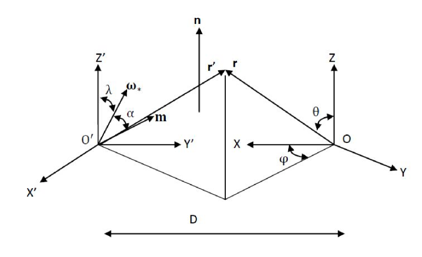
Figure 1: The coordinate systems adopted in this study for calculations. The $Oxyz$ coordinate system is anchored at the planet, with the origin $O$ at the planet’s center and $x$-axis pointing to the proto-star. On the other hand, the origin $O^{\prime}$ of the $O^{\prime}x^{\prime}y^{\prime}z^{\prime}$ system lies at the proto-star’s center with the $y^{\prime}$-axis pointing to $O$. The coordinate systems are the same as those in Laine et al. (2008). At $t=0$ the stellar spin $\mbox{\boldmath${\omega}$}_{*}$ is placed on the $y^{\prime}$-$z^{\prime}$ plane and is inclined at the obliquity angle $\lambda$ relative to the direction of the orbital axis $\bf n$ (i.e. the vertical axis $z^{\prime}$). As is viewed in the $Oxyz$ system co-moving with the planet, $\mbox{\boldmath${\omega}$}_{*}$ rotates around the vertical axis with the angle $\lambda$ at the rate of the orbital angular frequency $n$. Moreover, as the star spins, the stellar dipole moment $\bf m$ rotates around $\mbox{\boldmath${\omega}$}_{*}$ with the misaligned angle $\alpha$. We let the $y^{\prime}$ axis always secularly follow the precession of $\mbox{\boldmath${\omega}$}_{*}$ such that $\mbox{\boldmath${\omega}$}_{*}$ always lies on the $y^{\prime}$-$z^{\prime}$ during the secular evolution.

Following the same mathematical procedures in Laine et al. (2008), we solve the resistive induction equation in the co-moving frame of the planet, with the stellar dipole fields and the induced fields expressed in terms of the poloidal scalars $\phi_{*}({\bf r},t)$ and $\phi_{p}({\bf r},t)$, respectively: namely, the magnetic field B, which has a poloidal nature in our problem, is related to the poloidal scalars by B $=\nabla\times(\nabla\times(\phi\hat{\bf r}))$, where $\hat{\bf r}$ is the unit vector of r. The SI unit system is adopted to present the equations for electromagnetic calculations. The induced poloidal scalar $\phi_{p}$ can be solved by the separation of variables in the spherical coordinates ($r$, $\theta$, $\varphi$) of such a frame after $\phi_{*}$ and the resistivity profile $\eta(r)$ are given. Let $R_{p}$ be the planet radius. For notation convenience, we denote $\phi_{p}(r>R_{p})\equiv\phi_{p,out}$ and $\phi_{p}(r<R_{p})\equiv\phi_{in}$. Hence the total poloidal scalar outside of the planet is $\phi_{out}=\phi_{*}+\phi_{p,out}$. In the case of $\lambda=0$, $\phi_{*}$ and therefore $\phi_{p}$ vary at the rate equal to $\omega_{*}-n$ as viewed by the planet, where $\omega_{*}$ is the stellar spin angular frequency and $n$ is the orbital angular frequency of the planet. In the Appendix A, we illustrate the coordinate systems for the problem (see Figure 1) and derive the detailed equations to solve for the potential scalar induced by a tilted magnetic dipole in the presence of stellar obliquity. We show that in order to describe the time-varying potential, there will be 3 more frequencies involved other than $\omega_{-}\equiv\omega_{*}-n$; they are $\omega_{+}\equiv\omega_{*}+n$, $\omega_{*}$ and $n$. Once the potential scalar $\phi_{p}$ is solved, the induced magnetic field $=\nabla\times(\nabla\times\phi_{p}{\bf\hat{r}})$, the electric field $\bf E$, the electric current $\bf j$, and hence the Ohmic dissipation can be all calculated (Laine et al., 2008). In the following subsections, we describe how to calculate the resistivity of the planet and the corresponding spin and orbital evolutions due to the Ohmic dissipation in our model.

2.1 Calculation of resistivity

For a hot Jupiter around a T Tauri star of one solar luminosity, the equilibrium temperature is $\sim 1000-2000$ K at the photosphere. The gas in the region just below the photosphere is therefore weakly ionized due to thermal ionization of alkaline elements. As the temperature and density continue to rise in deep layers, the thermal ionization of the most abundant constituents H and He starts to become non-negligible. In the even deeper interior, the density is high enough so that the fluid is partially degenerate and fully ionized due to pressure ionization (Saumon et al., 1995). It has been shown that the electric currents and magnetic fields induced near the planet’s surface are only present in the outer part of the planet where the ionization fraction is low and hence the resistivity is high. That is, magnetic fields decrease significantly over a skin depth $\delta$ from the surface to the interior (Laine et al., 2008; Batygin & Stevenson, 2010). In other words, the induced electric currents and magnetic fields are considerably shielded out by the outer part of the planet such that the precise values of resistivity in the interior do not matter. Thus in this work, we restrict ourselves to the resistivity $\eta$ due to electron-neutral collisions in a weakly ionized plasma (Draine et al., 1983; Blaes & Balbus, 1994):

$$\eta_{e-n}=230\left({n_{n}\over n_{e}}\right)T^{1/2}\ {\rm cm^{2}/s},$$ (1)

and apply the above equation to the entire planet without making a significant error. In the above equation, $n_{n}$ is the neutral number density, $n_{e}$ is the electron number density, and $T$ is the temperature.

To estimate the ionization fraction in eq.(1), we first consider the thermal ionization of alkaline elements. Thermal ionization is governed by the Saha equation (cf. Blaes & Balbus, 1994; Perna et al., 2010)

$${n_{e}\over n_{n}}\approx{1\over n_{n}^{1/2}}\left({m_{e}kT\over 2\pi\hbar^{2}}\right)^{3/4}\sqrt{\sum_{j}f_{j}\exp{(-I_{j}/kT)}},$$ (2)

where $n_{e}=\sum n_{j}^{+}$, $n_{j}=f_{j}n$, $k$ is the Boltzmann’s constant, $\hbar$ is the Planck’s constant divided by $2\pi$, and $n_{j}^{+}\ll n_{j}$ is assumed. We follow Batygin & Stevenson (2010) to find the abundances $f_{j}$ and ionization potential $I_{j}$ of each alkaline species (labelled by $j$) inferred from Lodders (1999) and Cox & Pilachowski (2000).

In even deeper layers, the thermal ionization of the most abundant constituents H and He starts to dominate the electron contribution. We compute the H & He ionization based on the equation of state tables in Saumon et al. (1995). Given the pressure $P$, temperature $T$, and the helium mass fraction $Y$, the mass density is given by (Saumon et al., 1995)

$${1\over\rho(P,T)}={1-Y\over\rho^{H}(P,T)}+{Y\over\rho^{He}(P,T)},$$ (3)

where $\rho^{H}(P,T)$ and $\rho^{He}(P,T)$ are obtained from interpolation of the data in the EoS tables for pure H and He, respectively. Hence, the electron number density $n_{e}$ and the total number density $n$ are given by (see eqs.(36) & (37) in Saumon et al. 1995)

$$n_{e} = n_{e}^{H}+n_{e}^{He}={2\rho_{H}/m_{H}\over 1+3X_{H_{2}}+X_{H}}X_{e}^{H}+{3\rho_{He}/m_{He}\over 1+2X_{He}+X_{He^{+}}}X_{e}^{He},$$ (4)

$$n = n_{H_{2},H,H^{+},e}+n_{He,He^{+},He^{2+},e}={2\rho_{H}/m_{H}\over 1+3X_{H_{2}}+X_{H}}+{3\rho_{He}/m_{He}\over 1+2X_{He}+X_{He^{+}}},$$ (5)

where $\rho_{H}\approx\rho(1-Y)$, $\rho_{He}=\rho-\rho_{H}=Y\rho$, $X_{e}^{H}$ and $X_{e}^{He}$ are given by eqs.(34) and (35) respectively in Saumon et al. (1995). $Y=0.283$ is adopted in our interior-structure simulations.

2.2 Planet radius and spin-orbital evolution due to Ohmic heating

Including the Ohmic dissipation but neglecting the small planetary spin energy (Bodenheimer et al., 2001), we have the evolution of the global energy for the entire planet governed by (cf. Chang et al., 2010)

$$\dot{U}+\dot{W}=\dot{Q}_{ohmic}-L,$$ (6)

where $U$ is the internal energy, $W$ is the gravitational potential energy, $L$ is the intrinsic luminosity from the photosphere of the planet, and $\dot{Q}_{ohmic}$ is the Ohmic dissipation rate given by (Laine et al., 2008)

$$\dot{Q}_{ohmic}=\left\langle\int_{r\leq R_{p}}\mu_{0}\eta{\rm Re}({\bf j})^{2}dV\right\rangle=\left\langle\int_{r\leq R_{p}}{\eta\over\mu_{0}}[{\rm Re}(\nabla\times{\bf B})]^{2}dV\right\rangle,$$ (7)

where “Re” means taking the real part and $\langle\rangle$ denotes the time averaging over the time scale longer than the forcing periods; namely, it is the secular evolutions of the spin and orbit that are relevant to the long-term thermal evolution of the interior structure. $\dot{Q}_{ohmic}$ should be equal to the average flow of the electromagnetic power (i.e. the Poynting vector) into the planet through the planet’s photosphere (e.g. Jackson, 1990).

Owing to the diffusive nature of the problem, an order-of-magnitude estimate for the Ohmic dissipation can be made based on the dimensional analysis of Equation 7 with $\nabla\sim 1/\delta$ and $dV\sim R_{p}^{2}\delta$ (Campbell, 1997; Laine et al., 2008)

$$\dot{Q}_{ohmic}\sim{B^{2}\over 2\mu_{0}}(4\pi R_{p}^{2}\delta)\omega,$$ (8)

where the skin depth for our magnetic induction problem is $\delta=(2\eta/\omega)^{1/2}$, the stellar magnetic field near the planet is $B\sim(\mu_{0}/4\pi)m/D^{3}$, $\omega$ is the forcing frequency, $m$ is the magnitude of the stellar dipole moment, and $D$ the orbital separation (see Figure 1).

The spin-orbit evolution is dictated by the dissipation torque. The torque acting on the stellar spin due to the electromagnetic interaction in the inertial frame takes the form (cf. Campbell, 1997)

$${\bf T_{inert}=m_{obliquity,inert}\times B_{planet}(r=r_{star})}={\bf m_{obliquity,inert}}\times\nabla(\partial_{r}\phi_{p})_{\bf r=r_{star}}.$$ (9)

In the above equation, $\bf m_{obliquity,inert}$, given by ${\bf P_{x^{\prime}}m}$ (see the Appendix A), is the stellar dipole moment as seen in the inertial frame with n in the $z$-direction, and ${\bf B_{planet}}$ is the planet-induced magnetic field at the location of the star ${\bf r_{star}}=D{\bf\hat{i}}=D{\bf\hat{r}}+(\pi/2)\mbox{\boldmath${\hat{\theta}}$}$ (see Figure 1). Note that although ${\bf B_{planet}}$ is calculated in the planet’s rest frame, its value in the inertial frame is the same as in the non-relativistic regime when the terms of order $n^{2}D^{2}/c^{2}\ll 1$ are neglected, where $c$ is the speed of light (e.g. Thyagaraja & McClements, 2009).

We shall see that the stellar spin precesses secularly with time in the inertial frame and we are interested in the spin-orbit evolution on the secular timescale, much larger than the spin and orbital periods. This amounts to taking the time-average for each physical quantity to average out their short-term variations. Besides, it is convenient to work out the secular evolution problem in the precession coordinates with n always pointing to the $z$-direction. Hence after each time step, we switch to the inertial frame such that the stellar spin is always on the $y^{\prime}$-$z^{\prime}$ plane and the orbital angular momentum is always along the $z^{\prime}$-axis at the beginning of the next time step. We denote this “instantaneous” inertial frame as $O^{\prime}x^{\prime\prime}y^{\prime\prime}z^{\prime}$, which coincides with $O^{\prime}x^{\prime}y^{\prime}z^{\prime}$ at the beginning of each time step. Thus the time-averaged torque $\langle\bf T_{inert}\rangle$ in this inertial frame is given by (cf. Campbell, 1997)

$$\langle T_{x^{\prime\prime}}\rangle = m\langle\hat{m}_{z^{\prime}}B_{planet,r}-\hat{m}_{y^{\prime\prime}}B_{planet,\theta}\rangle,$$ (10)

$$\langle T_{y^{\prime\prime}}\rangle = m\langle\hat{m}_{x^{\prime\prime}}B_{planet,\theta}+\hat{m}_{z^{\prime}}B_{planet,\varphi}\rangle,$$ (11)

$$\langle T_{z^{\prime}}\rangle = -m\langle\hat{m}_{x^{\prime\prime}}B_{planet,r}+\hat{m}_{y^{\prime\prime}}B_{planet,\varphi}\rangle,$$ (12)

where $\hat{m}_{x^{\prime\prime}}$, $\hat{m}_{y^{\prime\prime}}$, and $\hat{m}_{z^{\prime}}$ are the three Cartesian components of the unit vector of $\bf m_{obliquity,inert}$.

Once the time-averaged torque is obtained in the inertial frame, we are ready to calculate the secular evolutions of spin and orbit. First of all, $\langle T_{x^{\prime\prime}}\rangle$ leads to the precession of stellar spin around the orbital axis; namely,

$$f(\lambda)I_{*}\omega_{*}{d\langle\varphi^{\prime\prime}\rangle\over dt}=\langle T_{x^{\prime\prime}}\rangle,$$ (13)

where $\langle\varphi^{\prime\prime}\rangle$ refers to the time-averaged precession angle and $f(\lambda)$ is a function of $\lambda$ given in the Appendix B. In the “instantaneous” inertial frame, $\langle{\bf T_{inert}}\rangle$ along the stellar axis determines $\dot{\omega}_{*}$. $-\langle T_{z^{\prime}}\rangle$ governs $\dot{n}$ and thus $\dot{D}$. Moreover, $\dot{\lambda}$ is caused by the components of $\langle T_{y^{\prime\prime}}\rangle$ and $\langle T_{z^{\prime}}\rangle$ normal to the stellar spin, and additionally by the back reaction $-\langle T_{y^{\prime\prime}}\rangle$ acting to the orbital angular momentum. In other words, using the “instantaneous” stellar spin $\mbox{\boldmath${\omega}$}_{*}=\omega_{*}\mbox{\boldmath${\hat{\omega}}$}_{*}=\omega_{*}(\sin\lambda{\bf\hat{j}^{\prime\prime}}+\cos\lambda{\bf\hat{k}^{\prime}})$, we arrive at a set of evolutionary equations:

$${d(I_{*}\omega_{*})\over dt}=\langle{\bf T_{inert}}\rangle\cdot\mbox{\boldmath${\hat{\omega}}$}_{*}=\langle T_{y^{\prime\prime}}\rangle\sin\lambda+\langle T_{z^{\prime}}\rangle\cos\lambda,$$ (14)

$${d\lambda\over dt}={\langle T_{y^{\prime\prime}}\rangle\cos\lambda-\langle T_{z^{\prime}}\rangle\sin\lambda\over I_{*}\omega_{*}}+{\langle T_{y^{\prime\prime}}\rangle\over M_{p}D^{2}n},$$ (15)

$$M_{p}{d(D^{2}n)\over dt}=-\langle T_{z^{\prime}}\rangle,$$ (16)

where $M_{p}$ is the planet’s mass and the complicated expression for $d\lambda/dt$ is explained in the Appendix B. The above 3 equations can be combined to express $\dot{\lambda}$ in terms of $\dot{L}_{spin}=d(I_{*}\omega_{*})/dt$ and $\dot{L}_{orb}=M_{p}d(D^{2}n)/dt$ as follows

$${d\lambda\over dt}={dL_{orb}\over dt}\left({1\over I_{*}\omega_{*}\sin\lambda}+{1\over M_{p}D^{2}n\tan\lambda}\right)+{dL_{spin}\over dt}\left({1\over I_{*}\omega_{*}\tan\lambda}+{1\over M_{p}D^{2}n\sin\lambda}\right),$$ (17)

which we shall find quite useful to interpret the evolutionary results.

Note that the moment of the inertia $I_{*}$ of the T Tauri star also evolves. In reality, $m$ evolves as well (Johns-Krull, 2007; Yang & Johns-Krull, 2011), but in this work we prescribe a constant value for $m$ for simplicity.

When $\lambda=0$, the terms in the magnetic potential scalar $\phi_{p}$ associated only with $\omega_{-}$ are left, leading to $\langle T_{x^{\prime\prime}}\rangle=\langle T_{y^{\prime\prime}}\rangle=0$. Therefore Equations (14)-(16) reduce to the ones in Campbell (1983):

$${d(I_{*}\omega_{*})\over dt} = \langle T_{z^{\prime}}\rangle,$$ (18)

$$M_{p}{d(D^{2}n)\over dt} = -\langle T_{z^{\prime}}\rangle.$$ (19)

In the absence of stellar obliquity, the torque and Ohmic heating can be simply related to each other by virtue of the equation $\dot{Q}_{ohmic}=|\omega_{-}\langle T_{z^{\prime}}\rangle|$ (Campbell, 1983; Laine et al., 2008). If $\lambda\neq 0$, we show in the §2.3 that the vector product ${\bf\langle T_{inert}\rangle}\cdot(\mbox{\boldmath${\omega}$}_{*}-{\bf n})$ gives rise to the Ohmic dissipation that drives the spin-orbit system toward a lower energy state. More specifically,

$$\dot{Q}_{ohmic} = -\left(\omega_{*}\langle T_{y^{\prime\prime}}\rangle\sin\lambda+\omega_{*}\langle T_{z^{\prime}}\rangle\cos\lambda-n\langle T_{z^{\prime}}\rangle\right),$$ (20)

$$= -\omega_{*}{dL_{spin}\over dt}+n{dL_{orb}\over dt}.$$ (21)

Since $\dot{Q}_{ohmic}$, $\omega_{*}$, and $n$ are all positive quantities in this work, the above equation indicates that $dL_{spin}/dt>dL_{orb}/dt$ for $\omega_{*}<n$ and vice versa, which is a familiar result for $\lambda=0$ but even applies generally to the cases for $\lambda\neq 0$. Note that even when $n=\omega_{*}$, $\dot{Q}_{ohmic}\neq 0$ due to the spin-orbit misalignment. In addition, $\langle T_{x^{\prime\prime}}\rangle$ causing the precession of stellar spin around the orbital axis does not do any mechanical work and thus is not related to the Ohmic dissipation in the planet.

In the special case where $\alpha=0$, the stellar dipole moment in the inertial frame is ${\bf\hat{m}_{obliquity,inert}}=(0,\sin\lambda,\cos\lambda)$. Substituting this into eqs.(11) & (12), we have the unique relation $\langle T_{z^{\prime}}\rangle/\langle T_{y^{\prime\prime}}\rangle=-\tan\lambda$ regardless of the value of $\omega_{*}$. This together with eq.(20) gives

$$\dot{Q}_{ohmic}=n\langle T_{z^{\prime}}\rangle,$$ (22)

which is independent of $\omega_{*}$ as it should be when the spin and stellar dipole are aligned. Once again, $\dot{Q}_{ohmic}>0$ and $n>0$ by our sign convention. It follows from the above equation that $\langle T_{z^{\prime}}\rangle>0$, therefore always leading to an orbit decay.

2.3 General relation between energy dissipation and torques

Since the torques arise from energy dissipation, we wish to derive the relation between the torques and dissipation in the presence of obliquity. This relation provides a powerful check on whether the Ohmic dissipation and the resulting torques calculated in §2.2 are correct.

The stellar spin angular momentum and planet’s orbital orbital angular moment are given by

$${\bf L_{spin}}=I_{*}\mbox{\boldmath${\omega}$}_{*},$$ (23)

and

$${\bf L_{orb}}=(m_{p}\sqrt{Gm_{*}a}){\bf\hat{n}},$$ (24)

respectively. Since the total angular momentum is conserved, ${\bf T^{\prime\prime}}=d{\bf L_{spin}}/dt=-d{\bf L_{orb}}/dt$.

However the total energy of the system is not conserved as a result of dissipation. The stellar spin energy changes at a rate according to

$${dE_{spin}\over dt}={d(1/2)I_{*}\mbox{\boldmath${\omega}$}_{*}^{2}\over dt}=\mbox{\boldmath${\omega}$}_{*}\cdot{dI_{*}\mbox{\boldmath${\omega}$}_{*}\over dt}=\mbox{\boldmath${\omega}$}_{*}\cdot{d{\bf L_{spin}}\over dt}.$$ (25)

The change rate of the orbital energy is

$${dE_{orb}\over dt}={GM_{*}m_{p}\over 2a^{2}}{da\over dt},$$ (26)

which can be linked to the change of the orbital angular momentum as follows

$${dE_{orb}\over dt}={d{\bf L_{orb}}\over dt}\cdot{\bf n}.$$ (27)

In deriving the above equation, we have taken the time derivative of Equation (24) and used the identity $d{\bf\hat{n}}/dt\cdot{\bf n}=0$. Thus

$$-\dot{Q}_{ohmic}\equiv{d(E_{spin}+E_{orb})\over dt}=\mbox{\boldmath${\omega}$}_{*}\cdot{d{\bf L_{spin}}\over dt}+{d{\bf L_{orb}}\over dt}\cdot{\bf n}={\bf T^{\prime\prime}}\cdot(\mbox{\boldmath${\omega}$}_{*}-{\bf n}).$$ (28)

Although the heating rate is expressed in terms of the Ohmic dissipation, the above relation for dissipative torques can apply generally to other dissipative processes such as tidal dissipation. It is apparent that we do not specify the Ohmic dissipation to deduce the above relation.

2.4 Summary of procedures

Given $I_{*}(t)$ and $M_{p}$, the evolutions of stellar spin and orbit ($\omega_{*}$, $\lambda$, and $D$) are coupled with the evolution of interior structure ($R_{p}$, $\eta(r)$ etc.) via the Ohmic dissipation in a hot Jupiter, which is modelled as a diamagnetic sphere in our calculation.

The procedure of the evolutionary calculations is summarized as follows. We start with initial $I_{*}$, $\omega_{*}$, $\lambda$, $D$, and $R_{p}$ to obtain $\dot{Q}_{Ohmic}$ and ${\bf T_{inert}}$. The next step consists of three calculations: the first is the calculation of the new interior structure of the young hot Jupiter due to $\dot{Q}_{Ohmic}$, the second is the computation of the new $I_{*}$ from a stellar code, and the last is the calculation of the new $\omega_{*}$, $\lambda$, $D$ from the integration of the ODEs from Equation (14) to Equation (16) based on ${\bf T_{inert}}$. Consequently, $I_{*}$, $\omega_{*}$, $\lambda$, $D$, and $R_{p}$ at the next time step will be obtained. Meanwhile, the computed $\bf T_{inert}$ and $\dot{Q}_{Ohmic}$ can be checked using Equation (20) to validate the calculation. The same procedure is then carried out over and over again to evolve the system until either the planet reaches its Roche radius or the calculation approaches the end of simulation at $10^{7}$ years. We employ the same codes described and used by Bodenheimer et al. (2001) and Chang et al. (2010) for the planetary and stellar interior structures, respectively.

To simulate the stellar rotation being locked by a process such as disk locking (e.g., see Chang et al., 2010, and reference therein), we also run cases (actually most of the cases) in which the stellar spin $\omega_{*}$ is held at its initial value throughout the simulation, even though $\lambda$ is still allowed to evolve by the magnetic interaction. It is conceivable that any external torques affecting $\omega_{*}$ should change $\lambda$ as well, such as the star-disk magnetic interaction by Lai (2012) and Foucart & Lai (2011). In this study, the star-disk interaction is not modelled with the star-planet magnetic interaction. Instead, we focus only on the evolutions due to the star-planet magnetic interaction, with the condition for $\omega_{*}$ to be “locked” for the sake of simplicity of the toy model.

3 Comparative studies without secular evolutions

In this section, we present a couple of test runs in our model without considering the evolution of spin, orbit, and interior structures of the proto-star and planet. The purpose of the test runs is to investigate how the Ohmic dissipation varies with $\lambda$ and $\alpha$. This provides parameter and thus comparative studies to understand the basic behavior of the results before we proceed to the more complicated calculations involving secular evolutions.

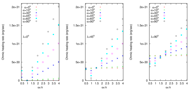
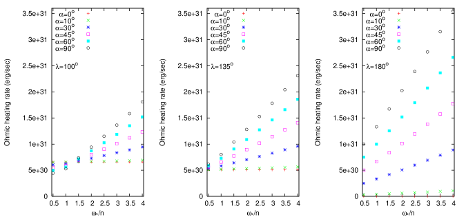
Figure 2: Dependence of the Ohmic heating rate on $\lambda$, $\alpha$, and $\omega_{*}/n$. The Ohmic heating rates are calculated from Equation(7). The mass, radius, and orbital radius of the young hot Jupiter are 1 Jupiter mass, 1.84 Jupiter radii, and 0.02 AU for this set of calculations.

Such comparative studies for the Ohmic dissipation rate $\dot{Q}_{ohmic}$ vs. $\omega_{*}/n$ are shown in Figure 2. $\dot{Q}_{ohmic}$ is calculated by virtue of Equation (7). We adopt $m=4\times 10^{34}$ A m², the same fiducial value used in Laine et al. (2008). The interior structure for a coreless hot Jupiter with $M_{p}=M_{J}$ and $R_{p}=1.84R_{J}$ is used for the test runs. We consider $\omega_{*}$ as a free parameter, whereas $n$ is held constant corresponding to the orbital radius of 0.02 AU. Thus, the stellar irradiation, which affects the interior structure, is also constant. This reduces the number of variables and helps to more easily examine how $\dot{Q}_{ohmic}$ varies with $\omega_{*}/n$ in the test runs. Everything else being the same, there is no difference in the Ohmic dissipation for $\alpha$ and for ($180^{\circ}-\alpha$) due to the axi-symmetry of dipole fields. Consequently, we only present the cases for $\alpha\leq 90^{\circ}$ in Figure 2.

The upper left panel of Figure 2 shows that in the absence of the stellar obliquity ($\lambda=0$), the Ohmic heating rates increase from zero for $\alpha=0$ to the maximum values for $\alpha=90^{\circ}$. In addition, the heating rate vanishes when $\omega_{-}=0$ (i.e. $\omega_{*}/n=1$) and increases with $|\omega_{-}|$ due to stronger electromagnetic interactions induced by faster forcing. The trend and the character of these results agree with those in Laine et al. (2008). The similar line of argument applies to the cases for $\lambda=180^{\circ}$ in which the stellar spin is completely flipped over and therefore the forcing frequency is $\omega_{+}$ rather than $\omega_{-}$. As illustrated in the lower right panel of Figure 2, the Ohmic heating rate increases with $\alpha$. Besides, the heating rate increases with $\omega_{*}$ and thus $\omega_{+}$.

We find that the dissipation torque $|T_{z^{\prime}}|$ for $\lambda=0^{\circ}$ decreases with the forcing frequency $|\omega_{-}|$ except when the forcing frequency is very close to zero; i.e. the torque peaks at $\omega_{-}\approx 1.3\times 10^{-4}$ s^-1 for $\lambda=0^{\circ}$. The maximum value of the torque arises because the torque is significantly weak for extremely slow forcing, and becomes small again for fast forcing due to the dissipation localized within one small skin depth below the planet’s surface (Campbell, 1983, 1997).

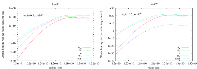
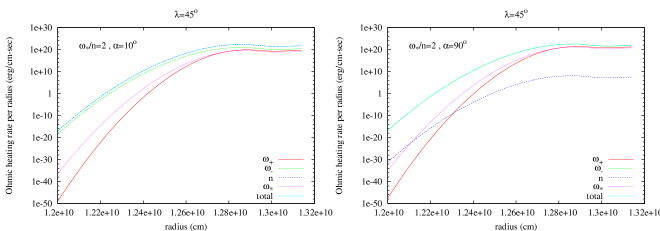
Figure 3: Ohmic heating rate profiles in a young hot Jupiter of 1 Jupiter mass and 1.84 Jupiter radii. $\alpha=10^{\circ}$ and $90^{\circ}$ for the stellar obliquity $\lambda=45^{\circ}$ are plotted. As illustrated in the figure, most of the Ohmic dissipation occurs in the outer part of the planet because the induced electromagnetic fields can only penetrate from the surface down over a length scale comparable to the skin depth $\sim\sqrt{\eta/\omega}$. The radiative-convective interface is located at $\approx 1.295\times 10^{10}$ cm. Note that the total heating profile overlaps with the profiles associated with other forcing frequencies (see the text in §3 for the details).

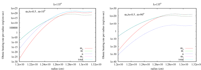
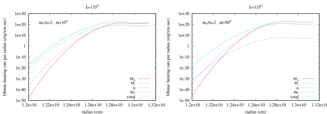
Figure 4: Same as Figure 3 but for a planet in a retrograde orbit with $\lambda=135^{\circ}$.

When $\lambda\neq 0$, the relation between $\omega_{*}$ and $\dot{Q}_{ohmic}$ becomes perplexing and requires more explanations. As shown in Figure 2 for $\lambda=45^{\circ}$, $90^{\circ}$, and $100^{\circ}$, the positive correlation between $\omega_{*}$ and $\dot{Q}_{ohmic}$ exists when $\omega_{*}/n$ is large enough for the forcing frequency $\omega_{*}$ to play the main role. This outcome can be realized by contemplating the problem in the two extreme regimes: $\alpha\gtrsim 0$ and $\alpha\lesssim 90^{\circ}$; the orbital motion alone contributes most of the heating in the former regime, whereas in the latter regime the Ohmic heating is generated primarily from the relative spin-orbit motion (i.e. $\omega_{-}$ or $\omega_{+}$ depending on $\lambda$). More specifically, Figure 2 shows that the heating rate is constant independent of $\omega_{*}$ for the cases of $\alpha=0$, in agreement with Equation (22); namely, the Ohmic dissipation induced entirely by the orbital motion with the forcing frequency $n$. As $\alpha$ starts to deviate from zero, we find that the Ohmic dissipations induced by other forcing frequencies begin to increase but the Ohmic heating arising solely from the orbital motion starts to decrease. This can been seen in Figures 3 & 4 for $\alpha=10^{\circ}$ where the total heating profile (shown in cyan line) near the planet surface almost overlaps with the one corresponding to the forcing frequency $n$ (dotted blue line), but the heat contributions from other frequencies other than $n$ are not totally negligible. When $\alpha=90^{\circ}$, the heat contribution from the forcing frequency $\omega_{+}$ or $\omega_{-}$ as a result of the relative spin-orbit motion totally dominates over that from the forcing frequency $n$; namely, in the outer part of the planet, the total heating profile (cyan line) almost coincides with the one for $\omega_{-}$ (dashed green line) in Figure 3 and for $\omega_{+}$ (magenta line) in Figure 4. It can be confirmed by Equations (A1) and (A3) that when $\alpha=90^{\circ}$, the forcing with the frequency $n$ disappears in the expression of the stellar magnetic dipole moment ${\bf\hat{m}_{obliquity}}$ and thus in the corresponding poloidal scalar $\phi_{*}$, leading to null contribution of the dissipation from the forcing frequency $n$. Therefore, the tiny dissipations for $\alpha=90^{\circ}$ shown in Figures 3 & 4 (i.e. dotted blue line) stem totally from numerical errors, which are too small to affect the results. Note that the dissipation occurs primarily in the outer part of the planet because the induced magnetic fields are mostly confined within one skin depth below the photosphere.

Given the above explanations, we are able to further elaborate the general dependence of $\dot{Q}_{ohmic}$ on $\lambda$ and $\alpha$ shown in Figure 2. Let’s first examine the cases for $\lambda=45^{\circ}$, $90^{\circ}$ and $100^{\circ}$. In these cases, the heating rate in the high frequency range $\omega_{*}/n>1.5$-2 increases with $\alpha$. Roughly speaking, it is because the primary forcing switches from the slow rate $n$ to the fast rate $\omega_{+}$ (for $\lambda\geq 90^{\circ}$) or $\omega_{-}$ (for $\lambda<90^{\circ}$) as $\alpha$ increases (see the $\omega_{*}/n=2$ case in Figure 3). The trend apparently reverses in the low frequency range $\omega_{*}/n<1.5$-2; namely, the heating rate decreases with the increasing $\alpha$ (see the $\omega_{*}/n=0.5$ case in Figure 3).

In contrast, for the retrograde orbits with large stellar obliquities as represented by the cases for $\lambda=135^{\circ}$ and $180^{\circ}$ in Figure 2, the Ohmic dissipation always increases with $\alpha$. The forcing with the frequency $\omega_{+}$ is always fast enough to induce more heat for larger $\alpha$ than the heat generated mostly by the slower forcing with the frequency $n$ for smaller $\alpha$. This consequence can be implied by comparing the heating profiles for $\omega_{*}/n=2$ with those for $\omega_{*}/n=0.5$ in Figure 4.

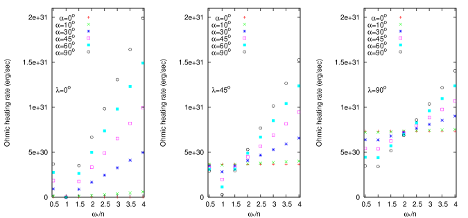
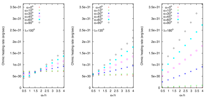
Figure 5: Same as Figure 2 but the Ohmic heating rates are computed from Equation (20).

To further validate our numerical calculations, we also compute $\dot{Q}_{ohmic}$ based on the general torque-dissipation relation given by Equation (20) and show the results in Figure 5. In general, Figure 2 and Figure 5 are consistent with each other. The discrepancy between the two types of calculations of $\dot{Q}_{ohmic}$ is $<7$%. In addition, the results of $\dot{Q}_{ohmic}$ can be crudely verified by Equation (8). Using $\eta=8.3\times 10^{9}$ m²/s, which is approximately the maximum value of the $\eta(r)$ profile in the calculations, we obtain the skin depth $\delta\approx 1.5\times 10^{9}$ cm. The substitution of this skip depth into Equation (8) gives the dissipation rate $\dot{Q}_{ohmic}\approx 2\times 10^{31}$ erg/s, which is on the similar order of the magnitude to those shown in Figure 2.

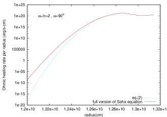
Figure 6: Comparison between the total heating profile derived from Equation (2) and that from the full version of the Saha equation for the cases corresponding to the top left (left in this figure) and bottom right (right in the figure) panels of Figure 3.

All the dissipation rates in the test runs have been calculated based on Equations (1) and (2) under the assumption of the low ionization fraction of each alkali species as well as the low total ionization fraction within the skin depth. To verify whether this assumption is reasonable in terms of the heat generation, we apply the full version of the Saha equation, e.g. Equation(1) in Batygin & Stevenson (2010), to the test runs. We find that the total ionization fraction is sufficiently low in the outer part of the planet such that Equation (1) still applies. We then compute the new heating rate profiles and compare them to those based on Equation (2). Figure 6 illustrates the comparisons for the two cases shown in the upper left and lower right panels of Figure 3 as the representative examples. It is evident from the figure that the heating profiles derived from Equation (2) and from the full version of the Saha equation are almost the same in the outer part of the planet where most of the dissipation occurs. It then follows that the total heating rates derived from the full version of the Saha equation are only 3-4% higher that those derived from Equation (2), thus validating the approximate results using Equation (2).

4 Evolutionary results

We now present the evolutionary results with the input parameters and different initial conditions listed in Table 1. The initial $\omega_{*}$ is given by one half of the initial $n$. This initial condition is based on the assumptions that the inner edge of the disk is located at the location of the co-rotation radius of the proto-star due to disk locking (e.g., see Chang et al., 2010, and reference therein) and that the initial location of the planet lies in the orbit with the 2:1 mean motion resonance with the inner edge of the disk according to planet migration theories (see Lin et al. 1996; Rice et al. 2008; cf. Benítez-Llambay et al. 2011). The simulation is run from $t_{i}=0.7$ to $t_{end}=10$ Myrs, corresponding to the T Tauri star phase. The starting time $0.7$ Myrs is comparable to the timescale of the type II migration time of a giant planet in a protoplanetary disk (Lin et al., 1996). Except for Case 1 which allows $\omega_{*}$ to evolve according to Equation (14) for comparison, we do not evolve $\omega_{*}$ in other cases as it is assumed to be locked by some process such as disk locking. We also run Case 20 with the parameters similar to the fiducial model in Laine et al. (2008): $M_{p}=0.63M_{J}$, $D_{i}=0.04$ AU, $\omega_{-}=10^{-5}$ s^-1, $\lambda=0^{\circ}$, $\alpha=90^{\circ}$, $M_{*}=M_{\odot}$, and $L_{*}=1.5L_{\odot}$. It should be stressed that even in an aligned system, the size of the magnetospheric inner cavity is proportional to $m^{4/7}{\dot{M}}^{-2/7}$, where $\dot{M}$ is the disk gas accretion rate onto the T Tauri star (e.g. see Lai, 1999, and references therein). In other words, the initial $n$ is in fact related to $m$ and $\dot{M}$. Moreover, $\omega_{*}$ evolves as the magnetospheric cavity evolves even in the disk-locking model. Since we assume a constant $m$ and do not intend to model the cavity size in the presence of stellar obliquity and the misaligned magnetic dipole, we simply parameterize the initial value of $n$ independent of $m$ in this work.

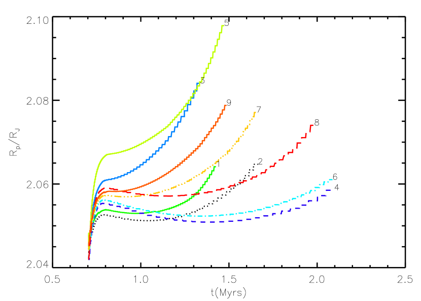
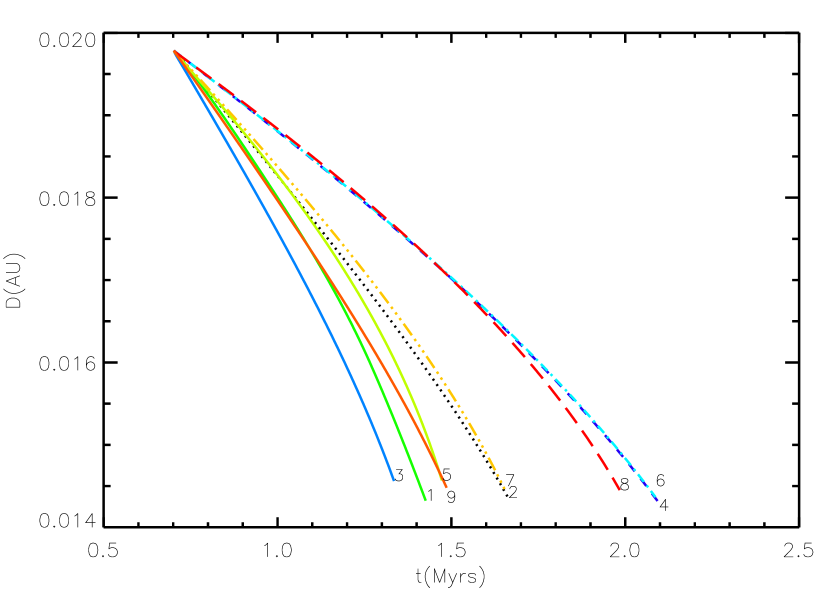
Figure 7: Coupled evolutions of $R_{p}$ and $D$ of the young hot Jupiter in Cases 1-9. The number labelled next to each curve is the case number. The evolutionary curves for Cases 4 and 6 are very similar.

Cases 1-9 represent the evolutions of a young hot Jupiter of 1 $M_{J}$ initially at the very close distance $D_{i}\approx 0.02$ AU, resembling a planet lying inside a small magnetospheric cavity. Owing to the small starting orbital distance, the strong Ohmic dissipations are generated on the order of $10^{30-31}$ erg/s throughout the evolutions, resulting in fast orbital decays. However, because the intense heating occurs mainly near the planet surface, the dissipation is unable to significantly inflate the planet against self-gravity. Figure 7 shows that the rise in $R_{p}$ is $<$ 3% in these cases when the planet quickly shrinks its orbit and fills its Roche lobe in just a few $10^{5}$ to about 1 million years after $t_{i}$. The small increase in $R_{p}$ arises from the thermal expansion of the outer part of the planet. Despite the intense heating near the planet surface, temperature inversion is not observed because the strong dissipation is limited to the radiative layer in the evolutionary cases and thus is easily lost. In these cases, the planet first undergoes relatively fast expansion as the dissipation is suddenly deposited in the beginning, and then reaches an intermediate quasi-equilibrium state (i.e. $\dot{Q}_{ohmic}\sim L$ in Equation 6) that lasts for some period of time depending on how fast the orbit decays. The planet expands again as the orbit continues to shrink and thus the Ohmic dissipation is further enhanced.

Among these cases, Cases 1, 2, and 3 present the evolutions in the absence of the stellar obliquity ($\lambda=0$). In Case 1, $\omega_{*}$ evolves, caused by the dissipation torques and $\dot{I}_{*}$ according to Equation (14), without the spin-locking assumption. In Cases 2 and 3, $\omega_{*}$ is constant. Figure 7 shows that $R_{p}$ and $D$ in Case 1 evolve faster than those in Case 2, starting from the same initial conditions. It is because the forcing frequency $|\omega_{-}|$ is lower in Case 1, leading to faster orbital decay as explained in §3. A larger skin depth results from the slower forcing, generating deeper heating and thus faster expansion. Figure 7 also shows that $R_{p}$ and $|\dot{D}|$ in Case 3 are always larger than that in Case 2 as expected from the test runs in §3; the larger $\alpha$ in Case 3 produces the stronger heating and faster orbital decay.

On the other hand, Cases 4, 5, and 6 present the studies in which $\lambda\neq 0$ but the stellar spin and dipole are parallel (i.e. $\alpha=0$). Although the stellar spins in Cases 4 and 6 point to opposite directions, Figure 7 shows that their evolutions of $R_{p}$ and $D$ are similar due to the similar time variation of the stellar dipole field that is axi-symmetric about the spin axis. Furthermore, the larger $R_{p}$ and $|\dot{D}|$ in Case 5 than those in Cases 4 and 6 is a result of the larger $\lambda$ and thus stronger heating, in accordance with the results of the test runs shown in the upper middle and upper right panels of Figure 2 for $\alpha=0^{\circ}$ and $\omega_{*}/n=0.5$. The almost symmetric evolutions between Cases 4 and 6 are broken when $\alpha\neq 0^{\circ}$, as illustrated by the different evolution curves for their counterpart cases 7 and 8.

We also run Case 9 to compare with Cases 4 and 7 to examine the evolutions starting from the same $\lambda_{i}=45^{\circ}$ but different $\alpha$. As has been demonstrated in §3, Case 9 lies in the special regime where $\alpha=90^{\circ}$ and hence no dissipation is contributed from the forcing frequency $n$, in contrast to the other extreme regime shown in Case 4 where the dissipation is totally from the forcing frequency $n$. The total dissipation rate and therefore $R_{p}$ as well as $|\dot{D}|$ increases with $\alpha$ in these cases during the evolutions, which is consistent with the result of the test run for $\lambda=45^{\circ}$ and $\omega_{*}/n=0.5$ displayed in Figure 2.

Table 1 shows that the stellar obliquity $\lambda$ remains zero in Cases 1-3 as expected, because $\langle T_{z^{\prime}}\rangle$ is the only component of the dissipation torque acting on the stellar spin. Moreover, $\lambda$ in Cases 4 and 6 change similarly; $\Delta\lambda\approx-11^{\circ}$ for both cases, meaning that the dissipation torques turn the system toward the spin-orbit alignment in Case 4 and toward the anti-alignment in Case 6 at similar rates. By contrast, $\lambda$ hardly alters in Case 5 when $\lambda_{i}=90^{\circ}$. In the presence of $\alpha$, the evolution of $\lambda$ is more complicated; the dissipation torques can either excite or damp the stellar obliquity. Table 1 shows that $\lambda$ in Cases 7 and 8 is decreased by about $2^{\circ}$-$3^{\circ}$, while $\lambda$ in Case 9 is increased by about $3^{\circ}$. The changes of $\lambda$ are nonetheless much slower than those in Cases 4 and 6.

The aforementioned evolutions of $\lambda$ for Cases 4-9 can be understood through examination of Equation (17). Because $\alpha=0$ in Cases 4-6, $dL_{spin}/dt=0$ and $dL_{orb}/dt<0$ in these cases as has been shown in §2. Equation (17) then indicates that the dissipation torques acting on the star are unable to spin up/down the star but contribute entirely to the evolution of $\lambda$. This explains why the evolutions of $\lambda$ in Cases 4 and 6 are faster than those in Cases 7, 8, and 9. Besides, we find that the orbital axis moves faster toward the stellar spin instead of the other way around. It is due to the fact that $M_{p}D^{2}n/I_{*}\omega_{*}\sim 0.1$-$0.01\ll 1$ in our model. Namely, it is the terms associated with $1/(M_{p}D^{2}n)$ rather than with $1/(I_{*}\omega_{*})$ on the right-hand side of Equation (17) (or equivalently Equation (15)) that dominate $\dot{\lambda}$. As a result, Equation (17) gives similar decreases in $\lambda$ in Cases 4 and 6. On the other hand in Case 5, $\lambda_{i}=90^{\circ}$ and hence only the terms with $1/(I_{*}\omega_{*})$ in Equation (17) exist at the beginning, which is negative and small. This explains why $\lambda$ hardly evolves in Case 5; namely, $\Delta\lambda$ is only $-0.02^{\circ}$. We can set Equation (17) equal to zero in the case of $\alpha=0$ and find the equilibrium orientation for the stellar spin, which gives $\lambda=\arccos(-M_{p}D^{2}n/I_{*}\omega_{*})\approx\pm 90^{\circ}$, consistent with the small $\dot{\lambda}$ in Case 5. The equilibrium is unstable as we can anticipate from Cases 4 and 6. Roughly speaking, the dissipation torque turns the stellar spin and the orbital axis toward alignment when $|\lambda|\leq 90^{\circ}$ and toward anti-alignment when $>90^{\circ}$.

When $\alpha\neq 0$, $dL_{spin}/dt$ becomes non-zero. In the case of $n>\omega_{*}$, $dL_{spin}/dt>0$ and $dL_{orb}/dt<0$. Equation (17) implies that for Cases 7, 8, and 9, the term associated with $dL_{orb}/dt$ damps $\lambda$, while the term with $dL_{spin}/dt$ excites $\lambda$. When $\alpha=0$, $dL_{spin}/dt=0$ and therefore the excitation term vanishes. As $\alpha$ increases from zero, the excitation term increases as well. This reiterates the point described in the above paragraph that $\lambda$ damps much more slowly when $\alpha=45^{\circ}$. When $\alpha=90^{\circ}$, it turns out that the excitation term dominates over the damping term, leading to $\dot{\lambda}>0$ in Case 9.

As we have seen, the values of $|\lambda|$ in Cases 4 and 6 change similarly. Indeed, inspection of Figure 7 reveals that the evolutions of $R_{p}$ and $D$ in Cases 4 and 6 are very similar. As has been described above, the reason is that their secular interactions are almost the same when the stellar dipole is aligned or anti-aligned with the stellar spin (i.e. $\alpha=0$).

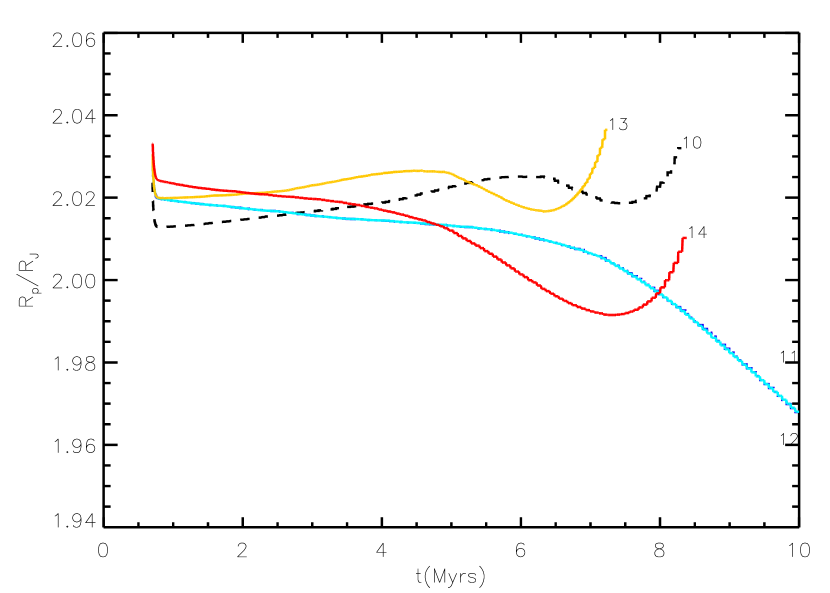
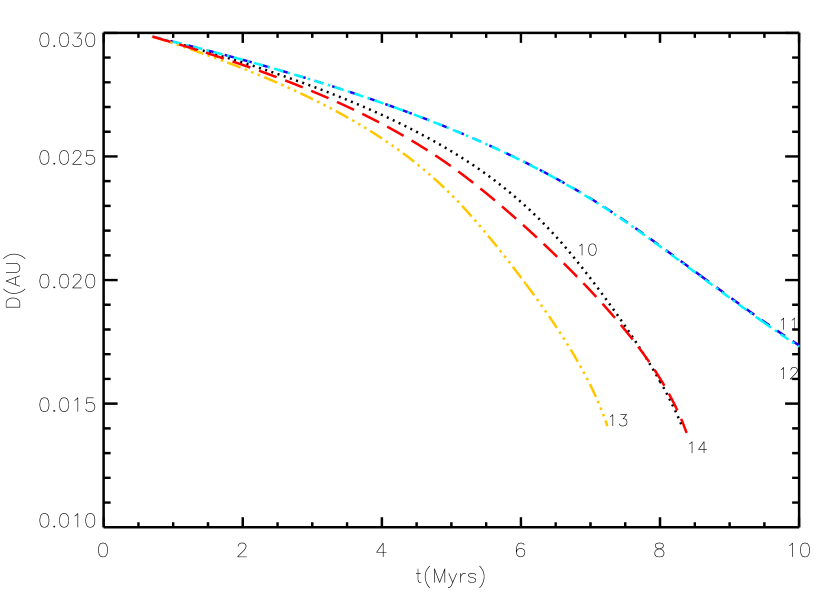
Figure 8: Coupled evolutions of $R_{p}$ and $D$ of the young hot Jupiter in Cases 10-14. The numbers labelled next to the curves indicate the different cases. The evolutionary curves for Cases 11 and 12 almost overlap.

Cases 10-14 present the evolutions of the planet placed initially at the farther distance $D_{i}\approx 0.03$ AU from its T Tauri star. Hence, the magnetic interaction and the resulting Ohmic dissipation are weaker at the beginning of the evolution (i.e. $\dot{Q}_{ohmic}\sim 10^{29}$ erg/s) than those in Cases 1-9. Consequently, the planet’s orbit decays to $D\lesssim 0.018$ AU over a timescale of a few Myrs as shown in Figure 8. Unlike the initial rise of $R_{p}$ in Cases 1-9, $R_{p}$ first decreases quickly over a short period of time, $\sim 10^{5}$ years in these cases. Then the planet undergoes a slow change of the size over a few Myrs, meaning that $\dot{Q}_{ohmic}\sim L$ in Equation (6) such that the radius is more or less maintained by the Ohmic dissipation at $R_{p}\sim 2$-$2.04R_{J}$. In addition, Figure 8 and Table 1 show that $D$, $R_{p}$, and $\dot{\lambda}$ of Cases 11 & 12 evolve almost identically, as expected for the same reason as the similarity between Cases 4 & 6. The stellar obliquities in Cases 11 & 12 decrease by a similar amount, about 20^∘ at the end of the simulation, but decrease only by about $5^{\circ}$ in Cases 13 & 14. The results are consistent with the comparative study for Cases 4, 6, 7, and 8; i.e., $\lambda$ decays faster when $\alpha=0$ in these cases. The faster decreases of $\lambda$ in Cases 11 & 12 give rise to the smaller heating rates than those in other cases during the late stages of the evolution, leading to faster contraction and slower orbital decay after $t\approx$ 6-7 Myrs. As a result, the planet in Cases 11 and 12 is unable to reach Roche-lobe overflow at the end of the simulation, whereas the planet in Cases 10, 13, and 14 migrates in fast enough to finally fill the Roche lobe during the T Tauri phase.

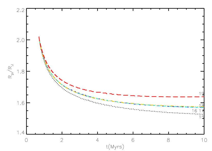
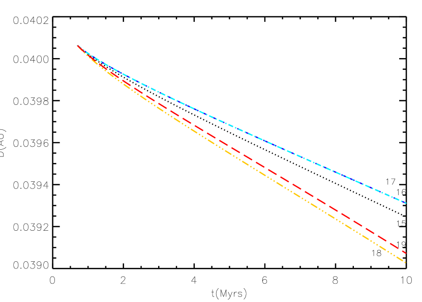
Figure 9: Coupled evolutions of $R_{p}$ and $D$ of the young hot Jupiter in Cases 15-19.

In Cases 15-19, we consider a young hot Jupiter initially on the even larger orbit at $D_{i}\approx 0.04$ AU. These cases correspond to the scenario that the planet lies in a large magnetospheric cavity. The larger the orbital distance is, the weaker the stellar magnetic fields and the interactions are. In all cases, the Ohmic dissipation rates are around $10^{28}$ erg/s throughout the simulation. As a result, the young planet first contracts and then gradually attains quasi-thermal equilibrium at small radii $R_{p}\approx 1.6R_{J}$ after $t\sim 4$-5 Myrs, as illustrated in Figure 9. The orbits do not decay to the distance $D<0.039$ AU from the star. Hence, the planet never reaches its Roche radius at the end of the simulation. The corresponding changes in $\lambda$ shown in Table 1 are much smaller as well in these cases.

Laine et al. (2008) focused on a planet that already fills its Roche lobe at $D_{i}=0.04$ AU (i.e. $R_{p}\approx 5R_{J}$), and calculated the resulting dissipation rate and mass loss rate. The interior structure of the planet is composed of an isothermal envelope and a polytropic core in their study, which does not truly take into account the energy equation. Although they suggested that the dissipation can inflate the planet and trigger mass loss through Roche lobe overflow, the authors cautioned that the initial condition of the Roche-lobe filling planet would not be valid. In Case 20, we apply our interior structure to the fiducial model of Laine et al. (2008) with the initial $R_{p}=2.045R_{J}$ at $t=t_{i}$. The evolutions of $R_{p}$ and $D$ are plotted in Figure 10. Since the planet is located outside the co-rotation orbital radius, the dissipation torque induced by the forcing $\omega_{-}>0$ drives the planet to migrate outwards. Although the planet in this case is less massive ($M_{p}=0.63M_{J}$) than in other cases ($M_{p}=1M_{J}$), the Ohmic heating is not strong enough to inflate the less massive planet to its Roche radius as suggested by Laine et al. (2008). Rather, the planet radius remains almost constant throughout the T Tauri phase.

5 Summary and discussions

We revisit the magnetic interaction between a hot Jupiter and its T Tauri star investigated by Laine et al. (2008). In the original work, the authors considered a Roche-lobe sized hot Jupiter without its own magnetic fields. The stellar spin was assumed to be aligned with the orbital axis; i.e. the stellar obliquity $\lambda=0$. As the planet orbits its parent star, the Ohmic dissipation in the planet is induced by the stellar magnetic dipole tilted away from the stellar spin with an angle $\alpha$. To calculate the electric resistivity of the planet, the interior structure was modelled as a sphere consisting of a polytropic core and an isothermal outer layer. In their model, the planet lies outside the co-rotating orbital radius such that the forcing frequency $\omega_{-}>0$. Based on their fiducial model, the authors suggested that the dissipation torques are not able to cause any significant orbital change. Nevertheless, the Ohmic heating occurring in the outer part of the planet is intense enough to inflate the planet up to the Roche radius. The mass loss through the Lagrangian 1 point toward the central star provides the angular momentum to the planet and thus possibly halts the planet migration in the disk.

Motivated by a wide range of the stellar obliquity detected in hot-Jupiter systems (e.g. Winn et al., 2011), which in theory could be excited during the T Tauri phase (Lai, 2012; Foucart & Lai, 2011), we extend the original model by considering the coupled evolution of the interior structure, planet’s orbit, and the stellar spin in the presence of the stellar obliquity $\lambda$. We focus on the secular evolution due to the dissipation torques and show that the Ohmic dissipation in the planet can be contributed linearly from the forcing associated with 4 frequencies: $\omega_{+}$, $\omega_{*}$, $n$, and $\omega_{-}$. Owing to the complication of the problem involving multiple frequencies, we begin with a couple of test runs based on a given interior structure for the dissipation calculation, which are further validated by the general torque-dissipation relation given by Equation (20) as well as the skin-depth estimation using Equation (8).

The coupled evolutions are then carried out for a number of cases listed in Table 1 for the purpose of parameter studies. The evolutions are computed from $t=0.7$ to $10$ Myrs. The radius of the coreless hot Jupiter of $1M_{J}$ is $2.045R_{J}$ at the beginning. Initially, the T Tauri star is assumed to spin at a rate $\omega_{*}=n/2$ to imitate the final stage of the planet migration scenario with a giant planet inside the magnetospheric cavity of the disk (Lin et al. 1996; Rice et al. 2008; cf. Benítez-Llambay et al 2011). Since the planet lies inside the co-rotating orbit, the planet continues to migrate inwards due to the Ohmic dissipation in the planet. Without modelling the star-disk magnetic interactions, the co-rotating orbit is simply assumed to correspond to the inner edge of the magnetically truncated disk despite the presence of $\lambda$ and $\alpha$. This is certainly one of the limitations of the study. In most of the cases, $\omega_{*}$ is assumed constant to simply resemble any processes, such as disk locking, that maintain the stellar spin.

Three initial orbital distances $D_{i}\approx 0.02$, 0.03, and 0.04 AU are considered. With our input parameters for $D_{i}\approx 0.02$ AU, the intense dissipation confined near the planet surface only enlarges $R_{p}$ by $<3$%. Nonetheless, the dissipation torques decay the orbit to the Roche zone in just a few $10^{5}$ to about 1 million years. The torques also evolve $\lambda$ when $\lambda_{i}\neq 0$. Since $M_{p}D^{2}n\ll I_{*}\omega_{*}$, $\dot{\lambda}$ is primarily contributed from the movement of the orbital axis rather than the stellar spin axis. When $\alpha$ is zero, there exists an unstable equilibrium for the orientation of the stellar spin axis, which points roughly about $90^{\circ}$ from the orbital axis. Consequently, the dissipation torques direct the orbital axis toward the stellar spin for a prograde orbit but toward the anti-parallel direction to the spin for a retrograde orbit. When $\alpha$ is non-zero, the orbital axis and the stellar spin can either evolve toward alignment/anti-alignment for small $\alpha$ or become more misaligned for $\alpha\lesssim 90^{\circ}$. Because the stellar spin is not spun up/down by the dissipation torque when $\alpha=0$, it follows that the stellar obliquity evolves more quickly when the stellar spin is parallel/anti-parallel to the stellar magnetic dipole.

For the young hot Jupiter initially at the farther distance $D_{i}\approx$ 0.03 AU, the dissipation is modest but still strong enough to more or less sustain the initial $R_{p}$ except for the cases with $\alpha=0$. The relatively fast decrease of $\lambda$ for $\alpha=0$ weakens the dissipation and the resulting torques, leading to the planet contraction and slow orbital decay in the late stage of the evolution. Therefore, in terms of the cases we have studied, the planet with $\alpha\neq 0$ undergoes substantial orbital decay in a few Myrs and finally overflows the Roche-lobe, while the planet with $\alpha=0$ can shrink its orbit but not sufficiently to allow for Roche-lobe overflow.

Owing to the weaker interaction at the larger orbital distance, the planet of 1 $M_{J}$ in all the cases starting from $D_{i}\approx 0.04$ AU contracts and then roughly reaches quasi-thermal equilibrium during the T Tauri phase, with the final $R_{p}$ smaller than those in the cases for $D_{i}\approx$ 0.02 and 0.03 AU. The corresponding orbital decays and the changes in the stellar obliquity are substantially smaller. The planet moves barely from its initial orbit and thus is not able to reach its Roche-lobe. We also carry out the simulation for the fiducial model in Laine et al. (2008) and find that the Ohmic heating can only sustain the radius of the less massive young hot Jupiter ($M_{p}=0.63M_{J}$), rather than thermally expanding the planet to its Roche radius as suggested by the authors.

The induced dissipation rates are as high as $10^{30-31}$ erg/s when the planet moves to about $D<$ 0.02 AU. The intense heating near the planet’s surface does not generate local temperature inversion in our model, in contrast to the surface heating models presented in Gu et al. (2004) and Wu & Lithwick (2012). It is probably because the dissipation responsible for the temperature inversion lies within a thin shell fairly deep in Gu et al. 2004 (a prescribed narrow Gaussian region) and in Wu & Lithwick 2012 (a region at about the optical depth of 100), while the dissipation in our diamagnetic induction model is deposited so close to the surface that it is easily lost and so there is no local maximum in T.

In this work, we introduce the planet at $t_{i}=0.7$ Myrs and adopt a constant magnetic dipole moment. In theory, a gas giant planet can form later and migrate to the magnetospheric cavity at a later time (e.g., Ida & Lin, 2008; Mordasini et al., 2009). Besides, the magnetic dipole moment may decay over the course of a few Myrs (Johns-Krull, 2007; Yang & Johns-Krull, 2011). Hence, our results probably give the suggestive values for the maximum changes of the stellar obliquity, orbital distance, and planet radius during the T Tauri star phase.

The orbital decay of a young hot Jupiter in our magnetic model is not significant unless the distance to the T Tauri star is smaller than about 0.03 AU. Some other process, such as gravitational tides (Chang et al., 2010) or a small magnetospheric cavity during FU-Orionis outbursts (Baraffe et al., 2009; Adams et al., 2009), can bring the planet in to that distance. The Ohmic mechanism could be the final stage in bringing a planet in very close to the T Tauri star or even leading to a Roche-lobe overflow. This may provide one of the explanations for the pile-up of hot Jupiters with the orbital periods of $\sim$ 3 days, and could also reduce the too-high population of hot Jupiters inferred from the population synthesis model (Ida & Lin, 2008). In this work, we do not study the post-evolution of a Roche-lobe filled planet. In terms of our model parameters, a young hot Jupiter located within 0.03 AU from its T Tauri star can undergo fast orbital decay on the timescales much shorter than 10 million years. Therefore it is possible that the young planet overflows its Roche lobe, migrates out, then migrates in, and overflows again. Consequently, the planet suffers from intermittent mass losses until its density is low enough to go through the stage of the runaway adiabatic mass loss (Chang et al., 2010), leading to the demise of the planet during the T Tauri phase.

As has been described in the Introduction, there is a large body of literature devoted to a variety of magnetic interactions between a hot Jupiter and its parent star, some of which can also cause the angular momentum to transfer between the planet’s orbit and the stellar spin. The efficiency of angular momentum transfer is model dependent, relying on the Ohmic dissipation rate. In the T Tauri phase, the presence of a disk is expected to magnetically affect the stellar spin and perhaps the planet’s orbit. Lai (2012) and Foucart & Lai (2011) considered a hybrid magnetic model including diamagnetic induction and magnetic-field linkage for the purpose of the generation of the stellar obliquity. In the study presented here, we follow the work by Laine et al. (2008) and therefore focus only on the diamagnetic interaction between the planet and its T Tauri star. Our simple model suggests that the stellar obliquity starting from a non-zero value may further evolve after the planet migrates into the magnetospheric cavity, making the orbit of the young hot Jupiter incline with the disk plane. As a result, a hot Jupiter does not necessarily lie on the same orbital plane with the planets farther out from the central star. Whether or not our model can provide a wide range of stellar obliquities at the end of T Tauri phase depends on the initial distribution of stellar obliquity as well as the distribution of the direction of stellar dipole moment relative to the stellar spin.

In the Introduction, we also caution that the skin depth beneath the photosphere is one of the major uncertainties of the model. In the presence of a planetary ionosphere or magnetosphere, the value may be appreciably smaller than what we compute in this work. Nevertheless, as an analog of the star-disk magnetic interactions (Lai, 1999), our diamagnetic model and other magnetic interactions should be considered together for the orbital evolution inside the magnetospheric cavity. While theoretical models are under development, it is conceivable in the future that photometric variability on timescales of a few days (e.g. Bouvier et al., 2007) and spectropolarimetry applied to T Tauri stars (e.g. Donati et al., 2008; Long et al., 2011) would serve as possible detection methods, to search for the variability modes and magnetic perturbations that are associated with the orbital motion of such a young hot Jupiter during the T Tauri star stage.

Appendix A magnetic scalar potential in the presence of stellar obliquity

We work on the problem with two sets of the coordinate systems $O^{\prime}x^{\prime}y^{\prime}z^{\prime}$ and $Oxyz$ illustrated in Figure 1, which were employed in Laine et al. (2008) with the orbital angular velocity and stellar spin around the $z$ (and $z^{\prime}$ axis). The magnetic dipole moment $\bf m$ is tilted with the angle $\alpha$ from the stellar spin and thus can be expressed as ${\bf m}=(\mu_{0}/4\pi)(B_{*}R_{*}^{3}/2){\bf\hat{m}}$ with the unit dipole moment vector ${\bf\hat{m}}=\sin\alpha\cos\omega_{*}t{\bf i^{\prime}}+\sin\alpha\sin\omega_{*}t{\bf j^{\prime}}+\cos\alpha{\bf k^{\prime}}$ as viewed in the star’s frame. Here $B_{*}$ is the surface stellar field and $R_{*}$ is the stellar radius. Then let the stellar spin rotate along the $x^{\prime}$ axis clockwise (counter-clockwise) on the $y^{\prime}$-$z^{\prime}$ plane such that the stellar obliquity angle is $\lambda>0$ ($<0$). This gives ${\omega_{*}}$ in the inertial frame of our problem. Note that the sign definition of $\lambda$ agrees with that used for the Rossiter-McLaughlin effect.

We then rotate the stellar spin along the $z^{\prime}$ axis clockwise at the angular velocity $n$ to give the stellar spin as observed in the co-moving frame of the planet. As a result, the unit vector of the stellar magnetic dipole moment $\bf\hat{m}_{obliquity}$ as viewed in the planet’s rest frame becomes

$${\bf\hat{m}_{obliquity}}={\bf P_{z^{\prime}}P_{x^{\prime}}\hat{m}}=\begin{pmatrix}\sin\alpha(\cos\omega_{*}t\cos nt+\cos\lambda\sin\omega_{*}t\sin nt)+\sin\lambda\cos\alpha\sin nt\\ \sin\alpha(-\cos\omega_{*}t\sin nt+\cos\lambda\sin\omega_{*}t\cos nt)+\sin\lambda\cos\alpha\cos nt\\ -\sin\lambda\sin\alpha\sin\omega_{*}t+\cos\lambda\cos\alpha\end{pmatrix}\,$$ (A1)

The rotation matrices involved in the above equations are

$${\bf P_{x^{\prime}}}=\left(\begin{array}[]{ccc}1&0&0\\ 0&\cos\lambda&\sin\lambda\\ 0&-\sin\lambda&\cos\lambda\end{array}\right),\qquad{\bf P_{z^{\prime}}}=\left(\begin{array}[]{ccc}\cos nt&\sin nt&0\\ -\sin nt&\cos nt&0\\ 0&0&1\end{array}\right).$$

Note that when the obliquity $\lambda=0$ in Equation (A1), we recover ${\bf\hat{m}}=\sin\alpha\cos\omega t{\bf i^{\prime}}+\sin\alpha\sin\omega t{\bf j^{\prime}}+\cos\alpha{\bf k}$ with the Doppler-shifted frequency $\omega$ being $\omega_{*}-n$ as viewed in the co-moving frame of the planet. Moreover, if the obliquity is retained but the magnetic axis is aligned with the stellar spin (i.e. $\alpha=0$), we obtain ${\bf\hat{m}_{obliquity}}=\sin\lambda\sin nt{\bf i^{\prime}}+\sin\lambda\cos nt{\bf j^{\prime}}+\cos\lambda{\bf k}$ as should be expected in the co-moving frame of the planet.

Then we can express the magnetic scalar potential due to the stellar magnetic dipole moment with non-zero stellar obliquity in the co-moving frame of the plane as follows (cf. Campbell, 1983):

$$V_{*} = {\mu_{0}m\over 4\pi r^{\prime 3}}{\bf r^{\prime}}\cdot{\bf\hat{m}}_{obliquity}$$ (A2)

$$= {\mu_{0}m\over 4\pi r^{\prime 3}}[r\sin\theta\sin\varphi\sin\alpha(\cos\omega_{*}t\cos nt+\cos\lambda\sin nt\sin\omega_{*}t)+r\sin\theta\sin\varphi\sin nt\sin\lambda\cos\alpha$$

$$+(D-r\sin\theta\cos\varphi)\sin\alpha(-\sin nt\cos\omega_{*}t+\cos\lambda\cos nt\sin\omega_{*}t)$$

$$+(D-r\sin\theta\cos\varphi)\sin\lambda\cos\alpha\cos nt+r\cos\theta(-\sin\lambda\sin\alpha\sin\omega_{*}t+\cos\lambda\cos\alpha)]$$

$$\approx {\mu_{0}mr\over 4\pi D^{3}}\{-P_{1}^{1}[{1\over 2}\sin\varphi\sin\alpha((\cos\omega_{+}t+\cos\omega_{-}t)+\cos\lambda(\cos\omega_{-}t-\cos\omega_{+}t))$$

$$+\sin\varphi\sin nt\sin\lambda\cos\alpha$$

$$+\cos\varphi\sin\alpha((\sin\omega_{-}t-\sin\omega_{+}t)+\cos\lambda(\sin\omega_{+}t+\sin\omega_{-}t))$$

$$+2\cos\varphi\sin\lambda\cos\alpha\cos nt]-P_{1}^{0}\sin\lambda\sin\alpha\sin\omega_{*}t\}$$

$$+{3\mu_{0}mr^{2}\over 8\pi D^{4}}\{P_{2}^{2}[{1\over 6}\sin 2\varphi\sin\alpha((\cos\omega_{+}t+\cos\omega_{-}t)+\cos\lambda(\cos\omega_{-}t-\cos\omega_{+}t))$$

$$+{1\over 3}\sin 2\varphi\sin nt\sin\lambda\cos\alpha$$

$$+{1\over 4}\cos 2\varphi\sin\alpha((\sin\omega_{-}t-\sin\omega_{+}t)+\cos\lambda(\sin\omega_{+}t+\sin\omega_{-}t))$$

$$+{1\over 2}\cos 2\varphi\sin\lambda\cos\alpha\cos nt]$$

$$-P_{2}^{0}[{1\over 2}\sin\alpha((\sin\omega_{-}t-\sin\omega_{+}t)+\cos\lambda(\sin\omega_{+}t+\sin\omega_{-}t))+\sin\lambda\cos\alpha\cos nt]$$

$$+{2\over 3}P_{2}^{1}\cos\varphi\sin\lambda\sin\alpha\sin\omega_{*}t\}$$

where $\omega_{+}\equiv\omega_{*}+n$, $\omega_{-}\equiv\omega_{*}-n$, and the approximation of $V_{*}$ is obtained by the expansion of $r^{\prime-3}$ up to the order of $(r/D)^{2}$. In the above equation, the time-independent terms are dropped out because they do not contribute to the electromagnetic induction. Besides, $P_{l}^{|m|}$ are associated Legendre functions, defined by $P_{1}^{0}=\cos\theta$, $P_{1}^{1}=-\sin\theta$, $P_{2}^{0}=(1/2)(3\cos^{2}\theta-1)$, $P_{2}^{1}=-3\sin\theta\cos\theta$, and $P_{2}^{2}=3\sin^{2}\theta$.

Using $V_{*}=-\partial_{r}\phi_{*}$, we have the poloidal scalar of the stellar field as follows

$$\phi_{*} = {\mu_{0}mr^{2}\over 8\pi D^{3}}\{P_{1}^{1}[{1\over 2}\sin\varphi\sin\alpha((\cos\omega_{+}t+\cos\omega_{-}t)+\cos\lambda(\cos\omega_{-}t-\cos\omega_{+}t))$$ (A3)

$$+\sin\varphi\sin nt\sin\lambda\cos\alpha$$

$$+\cos\varphi\sin\alpha((\sin\omega_{-}t-\sin\omega_{+}t)+\cos\lambda(\sin\omega_{+}t+\sin\omega_{-}t))$$

$$+2\cos\varphi\sin\lambda\cos\alpha\cos nt]+P_{1}^{0}\sin\lambda\sin\alpha\sin\omega_{*}t\}$$

$$+{\mu_{0}mr^{3}\over 8\pi D^{4}}\{-P_{2}^{2}[{1\over 6}\sin 2\varphi\sin\alpha((\cos\omega_{+}t+\cos\omega_{-}t)+\cos\lambda(\cos\omega_{-}t-\cos\omega_{+}t))$$

$$+{1\over 3}\sin 2\varphi\sin nt\sin\lambda\cos\alpha$$

$$+{1\over 4}\cos 2\varphi\sin\alpha((\sin\omega_{-}t-\sin\omega_{+}t)+\cos\lambda(\sin\omega_{+}t+\sin\omega_{-}t))$$

$$+{1\over 2}\cos 2\varphi\sin\lambda\cos\alpha\cos nt]$$

$$+P_{2}^{0}[{1\over 2}\sin\alpha((\sin\omega_{-}t-\sin\omega_{+}t)+\cos\lambda(\sin\omega_{+}t+\sin\omega_{-}t))+\sin\lambda\cos\alpha\cos nt]$$

$$-{2\over 3}P_{2}^{1}\cos\varphi\sin\lambda\sin\alpha\sin\omega_{*}t\}.$$

Note that we recover the original form of the poloidal scalar $\phi_{*}$ in Laine et al. (2008) when $\lambda=0$. In addition, because there is a poloidal scalar outside the planet $\phi_{p}$ generated by the fields induced by $\phi_{*}$ inside the planet, $\phi_{p}$ has the same time and angular dependence as $\phi_{*}$. Hence, $\phi_{p}$ is given by

$$\phi_{p}(r\geq R_{p},t)={\mu_{0}P_{1}^{0}\over r}(\delta_{1}\sin\omega_{*}t+\delta_{2}\cos\omega_{*}t)$$

$$+\mu_{0}P_{1}^{1}[{\sin\varphi\over r}(\alpha_{1}\sin\omega_{+}t+\alpha_{2}\cos\omega_{+}t+\alpha_{3}\sin\omega_{-}+\alpha_{4}\cos\omega_{-}t+\alpha_{5}\sin nt+\alpha_{6}\cos nt)$$

$$+{\cos\varphi\over r}(\alpha_{7}\sin\omega_{+}t+\alpha_{8}\cos\omega_{+}t+\alpha_{9}\sin\omega_{-}t+\alpha_{10}\cos\omega_{-}t+\alpha_{11}\sin nt+\alpha_{12}\cos nt)]$$

$$+{\mu_{0}P_{2}^{0}\over r^{2}}(\beta_{1}\sin\omega_{+}t+\beta_{2}\cos\omega_{+}t+\beta_{3}\sin\omega_{-}t+\beta_{4}\cos\omega_{-}t+\beta_{5}\sin nt+\beta_{6}\cos nt)$$

$$+\mu_{0}P_{2}^{1}{\cos\varphi\over r^{2}}(\epsilon_{1}\sin\omega_{*}t+\epsilon_{2}\cos\omega_{*}t)$$

$$+\mu_{0}P_{2}^{2}[{\sin 2\varphi\over r^{2}}(\gamma_{1}\sin\omega_{+}t+\gamma_{2}\cos\omega_{+}t+\gamma_{3}\sin\omega_{-}t+\gamma_{4}\cos\omega_{-}t+\gamma_{5}\sin nt+\gamma_{6}\cos nt)$$

$$+{\cos 2\varphi\over r^{2}}(\gamma_{7}\sin\omega_{+}t+\gamma_{8}\cos\omega_{+}t+\gamma_{9}\sin\omega_{-}t+\gamma_{10}\cos\omega_{-}t+\gamma_{11}\sin nt+\gamma_{12}\cos nt)].$$ (A4)

The above form for $\phi_{*}$ along with the separation of variables for the solutions to the induction equation suggest that the induced potential scalar $\phi_{p}$ can be in general given by

$$\phi({\bf r},t) = \Sigma_{l,m}C{{}_{l}^{m}}_{,\omega_{+}}G_{l,\omega_{+}}(r)Y_{l}^{m}(\theta,\varphi)e^{i\omega_{+}t}+\Sigma_{l,m}C{{}_{l}^{m}}_{,\omega_{-}}G_{l,\omega_{-}}(r)Y_{l}^{m}(\theta,\varphi)e^{i\omega_{-}t}$$ (A5)

$$+\Sigma_{l,m}C{{}_{l}^{m}}_{,\omega_{*}}G_{l,\omega_{*}}(r)Y_{l}^{m}e^{i\omega_{*}t}+\Sigma_{l,m}C{{}_{l}^{m}}_{,nt}G_{l,n}(r)Y_{l}^{m}(\theta,\varphi)e^{int}.$$

When $\lambda=0$, the above expression is reduced to only one term that is associated with $\omega_{-}$.

Inside the planet ($r\leq R_{p}$), the $r$-dependence of $\phi_{p}$ is given by

$$\left[{d^{2}\over dr^{2}}-\left({l(l+1)\over r^{2}}+{i\omega\over\eta}\right)\right]G_{l,\omega}(r)=0,$$ (A6)

where the forcing frequency $\omega$ denotes $\omega_{+}$, $\omega_{-}$, $\omega_{*}$, or $n$. If $\eta(r)$ is known, the above equation with each frequency can be solved by rearranging the equation to 4 first-order ODEs as have shown in Equation (10) of Laine et al. (2008), subject to the boundary conditions

$$G^{\prime}_{l}(R_{p})+{l\over R_{p}}G_{l}(R_{p})-(2l+1)R_{p}^{l}=0,$$ (A7)

$$G^{\prime}_{l}(r\approx 0)-{l+1\over r}G_{l}(r\approx 0)=0,$$ (A8)

After obtaining the solutions for $G_{l,\omega}$, we are ready to solve for the coefficients in the expressions of $\phi_{p}(r\leq R_{p},t)$ and $\phi_{p}(r\geq R_{p},t)$ by demanding the condition that the potential scalars and their derivatives should continue at $r=R_{p}$ for each frequency. Namely, $\phi_{*}+\phi_{p,out}=\phi_{p,in}$ and $\partial_{r}(\phi_{*}+\phi_{p,out})=\partial_{r}\phi_{p,in}$ at $r=R_{p}$ for each frequency. As a result, the terms associated with $\omega_{+}$ contribute 10 algebraic equations from $Y_{1}^{\pm 1}e^{i\omega_{+}t}$, $Y_{2}^{0}e^{i\omega_{+}t}$, and $Y_{2}^{\pm 2}e^{i\omega_{+}t}$. Likewise, the terms depending on $\omega_{-}$ and $n$ give rise to 10 algebraic equations each. On the other hand, the terms with $\omega_{*}$ only contribute 6 algebraic equations from $Y_{1}^{0}e^{i\omega_{*}t}$ and $Y_{2}^{\pm 1}e^{i\omega_{*}t}$, but keep in mind that the two terms associated with $\sin\varphi$ from $Y_{2}^{\pm 1}e^{i\omega_{*}t}$ should vanish as they do not exist in $\phi_{p}$, leading to the relation between $C{{}_{2}^{1}}_{,\omega_{*}}$ and $C{{}_{2}^{-1}}_{,\omega_{*}}$ (i.e. $6C{{}_{2}^{1}}_{,\omega_{*}}=C{{}_{2}^{-1}}_{,\omega_{*}}$) and hence reducing to 4 equations. Including their derivatives counterparts, we shall solve 20 algebraic equations for the 20 coefficients associated with $\omega_{+}$, $\omega_{-}$, and $n$. Besides, 8 equations for the 8 coefficients associated with $\omega_{*}$. In the end, we have 68 algebraic equations at $r=R_{p}$ and solve for the 68 coefficients, which are $\delta_{1,2}$, $\alpha_{1,\cdots 12}$, $\beta_{1,\cdots 6}$, $\epsilon_{1,2}$, $\gamma_{1,\cdots 12}$, Re$(C{{}_{1}^{\pm 1}}_{,\omega_{+},\omega_{-},n})$, Im$(C{{}_{1}^{\pm 1}}_{,\omega_{+},\omega_{-},n})$, Re$(C{{}_{2}^{0}}_{,\omega_{+},\omega_{-},n})$, Im$(C{{}_{2}^{0}}_{,\omega_{+},\omega_{-},n})$, Re$(C{{}_{2}^{\pm 2}}_{,\omega_{+},\omega_{-},n})$, Im$(C{{}_{1}^{\pm 1}}_{,\omega_{+},\omega_{-},n})$, Re$(C{{}_{1}^{0}}_{,\omega_{*}})$, Im$(C{{}_{1}^{0}}_{,\omega_{*}})$, Re$(C{{}_{2}^{1}}_{,\omega_{*}})$, and Im$(C{{}_{2}^{1}}_{,\omega_{*}})$. Then we know $\phi_{p,out}$ and $\phi_{p,in}$.

Appendix B Secular evolutions of the precession and obliquity of the stellar spin

While the stellar spin and the planet’s orbit exchanges angular momentum due to the dissipative torques in our magnetic model, the total angular momentum vector is conserved. Bearing this in mind, we have the secular evolution of the precession angle governed by (cf. Goldreich & Peale, 1970)

$$\sin\lambda_{*}I_{*}\omega_{*}{d\langle\varphi^{\prime\prime}\rangle\over dt}=\langle T_{x^{\prime\prime}}\rangle,$$ (B1)

where $\lambda_{*}$ is the angle between the stellar spin and the total angular momentum. Since the stellar spin angular momentum, orbital angular momentum, and total angular momentum form a vector triangle, it is straightforward to show from the triangle that

$$\sin\lambda_{*}={\sin\lambda\over\sqrt{(I_{*}\omega_{*}/M_{p}D^{2}n)^{2}+1+2(I_{*}\omega_{*}/M_{p}D^{2}n)\cos\lambda}}\equiv f(\lambda).$$ (B2)

This equation yields the expression of $f(\lambda)$ in Equation(13).

Now we turn to the evolution of the stellar obliquity. We define $d\lambda_{*}/dt$ and $d\lambda_{n}/dt$ as the contributions to the secular evolution of $\lambda$ due respectively to the stellar spin and orbital angular momentum moving toward/away from the total angular momentum. As has been described in the main text, $\dot{\lambda}$ is caused by the components of $\langle T_{y^{\prime\prime}}\rangle$ and $\langle T_{z^{\prime}}\rangle$ normal to the stellar spin and by the back reaction $-\langle T_{y^{\prime\prime}}\rangle$ acting to the orbital angular momentum. Hence we have (cf. Goldreich & Peale, 1970; Lai, 1999)

$$I_{*}\omega_{*}{d\lambda_{*}\over dt}=\langle T_{y^{\prime\prime}}\rangle\cos\lambda-\langle T_{z^{\prime}}\rangle\sin\lambda,$$ (B3)

$$M_{p}D^{2}n{d\lambda_{n}\over dt}=\langle T_{y^{\prime\prime}}\rangle.$$ (B4)

Therefore the equation

$${d\lambda\over dt}={d\lambda_{*}\over dt}+{d\lambda_{n}\over dt},$$ (B5)

gives the expression in Equation (15).

When $M_{p}D^{2}n\gg I_{*}\omega_{*}$, $\lambda_{*}\approx\lambda$ and $\dot{\lambda}_{*}\approx\dot{\lambda}$ as they ought to be because the total angular momentum is almost contributed from the orbital angular momentum. However, $M_{p}D^{2}n<I_{*}\omega_{*}$ for a system consisting of a hot Jupiter and a T Tauri star. As a result, the planet’s orbit can evolve more significantly than the stellar spin.

Table 1: model calculations. $m=4\times 10^{34}$ A m², $M_{p}=1M_{J}$, $M_{*}=1M_{\odot}$, $L_{*}=L_{\odot}$. The subscript $i$ denotes the initial value, while the subscript $f$ means the final value due to either the planet reaching its Roche lobe or $t=t_{end}$. In addition, at $t_{i}$, $R_{p}=2.045R_{J}$, $\langle\phi^{\prime\prime}\rangle=0$. The column “overflow” indicates in which cases the planet reaches the Roche-lobe overflow before $t=t_{end}$. The figure number for the results of each case is indicated in the column “Figure”.

Case	$D_{i}$ (AU)	$\alpha$	$\lambda_{i}$	$\lambda_{f}$	overflow	Figure
1	0.02	$45^{\circ}$	$0^{\circ}$	0∘	yes	7
2	0.02	$45^{\circ}$	$0^{\circ}$	0∘	yes	7
3	0.02	$90^{\circ}$	$0^{\circ}$	0∘	yes	7
4	0.02	$0^{\circ}$	$45^{\circ}$	$33.77^{\circ}$	yes	7
5	0.02	$0^{\circ}$	$90^{\circ}$	$89.98^{\circ}$	yes	7
6	0.02	$0^{\circ}$	$-135^{\circ}$	$-146.02^{\circ}$	yes	7
7	0.02	$45^{\circ}$	$45^{\circ}$	43.26∘	yes	7
8	0.02	$45^{\circ}$	$-135^{\circ}$	$-137.97^{\circ}$	yes	7
9	0.02	$90^{\circ}$	$45^{\circ}$	$48.25^{\circ}$	yes	7
10	0.03	$45^{\circ}$	$0^{\circ}$	0∘	yes	8
11	0.03	$0^{\circ}$	$45^{\circ}$	$21.97^{\circ}$	no	8
12	0.03	$0^{\circ}$	$-135^{\circ}$	$-157.89^{\circ}$	no	8
13	0.03	$45^{\circ}$	$45^{\circ}$	$40.56^{\circ}$	yes	8
14	0.03	$45^{\circ}$	$-135^{\circ}$	$-141.13^{\circ}$	yes	8
15	0.04	$45^{\circ}$	$0^{\circ}$	$0^{\circ}$	no	9
16	0.04	$0^{\circ}$	$45^{\circ}$	$44.44^{\circ}$	no	9
17	0.04	$0^{\circ}$	$-135^{\circ}$	$-135.55^{\circ}$	no	9
18	0.04	$45^{\circ}$	$45^{\circ}$	$44.88^{\circ}$	no	9
19	0.04	$45^{\circ}$	$-135^{\circ}$	$-135.16^{\circ}$	no	9
20	0.04	$90^{\circ}$	$0^{\circ}$	$0^{\circ}$	no	10

Figure 10: Coupled evolutions of $R_{p}$ and $D$ of the young hot Jupiter in Case 20.

References

- Adams (2011) Adams, F. 2011, ApJ, 730, 27
- Adams et al. (2009) Adams, F. C., Cai, M. J., & Lizano, S. 2009, ApJ, 702, 182
- Baraffe et al. (2009) Baraffe, I., Chabrier, G., & Gallardo, J. 2009, ApJ, 702, 27
- Batygin & Stevenson (2010) Batygin, K., & Stevenson, D. J. 2010, ApJ, 714, 238
- Batygin et al. (2011) Batygin, K., Stevenson, D. J., & Bodenheimer, P. H. 2011, ApJ, 738, 1
- Benítez-Llambay et al. (2011) Benítez-Llambay, P., Masset, F. & Beaugé, C. 2011, A&A, 528, 2
- Blaes & Balbus (1994) Blaes, O. M., & Balbus, S. A. 1994, ApJ, 421, 163
- Bodenheimer et al. (2001) Bodenheimer, P., Lin, D. N. C., & Mardling, R. A. 2001, ApJ, 548, 466
- Bouvier et al. (2007) Bouvier et al. 2007, A&A, 463, 1017
- Campbell (1983) Campbell, C. G. 1983, MNRAS, 205, 1031
- Campbell (1997) Campbell, C. G. 1997, “Magnetohydrodynamicss in Binary Stars”, Kluwer Academic Publishers
- Campbell (2005) Campbell, C. G. 2005, MNRAS, 359, 835
- Chang et al. (2010) Chang, S.-H., Gu, P.-G. & Bodenheimer, P. H. 2010, ApJ, 708, 1692
- Chatterjee et al. (2008) Chatterjee, S., Ford, E. B., Matsumura, S. & Rasio, F. A. 2008, ApJ, 686, 580
- Cox & Pilachowski (2000) Cox, A. N., & Pilachowski, C. A. 2000, Physics Today, 53, 77
- Dobbs-Dixon et al. (2010) Dobbs-Dixon, I., Cumming, A., & Lin, D. N. C. 2010, ApJ, 710, 1395
- Donati et al. (2008) Donati, J.-F. et al. 2008, MNRAS, 386, 1234
- Draine et al. (1983) Draine, B. T., Roberge, W. G., & Dalgarno, A. 1983, ApJ, 264, 485
- Foucart & Lai (2011) Foucart, F., & Lai, D. 2011, MNRAS, 412, 2799
- Gu et al. (2003) Gu, P.-G., Lin, D. N. C., & Bodenheimer, P. H. 2003, ApJ, 588, 509
- Gu et al. (2004) Gu, P.-G., Bodenheimer, P. H., & Lin, D. N. C. 2004, ApJ, 608, 1076
- Goldreich & Lynden-Bell (1969) Goldreich, P., & Lynden-Bell, D. 1969, ApJ, 156, 59
- Goldreich & Peale (1970) Goldreich, P., & Peale, S. J. 1970, AJ, 75, 273
- Hut (1981) Hut, P. 1981, A&A, 99, 126
- Ida & Lin (2008) Ida, S., & Lin, D. N. C. 2008, ApJ, 685, 584
- Jackson (1990) Jackson, J. D. 1990, “Classical Electrodynamics”, 2nd ed., John Wiley & Sons, U.S.A.
- Johns-Krull (2007) Johns-Krull, C. M. 2007, ApJ, 664, 975
- Kopp et al. (2011) Kopp, A., Schilp, S., & Preusse, S. 2011, ApJ, 729, 116
- Lai (1999) Lai, D. 1999, ApJ, 524, 1030
- Lai (2012) Lai, D. 2012, MNRAS, 423, 486
- Laine et al. (2008) Laine, R. O., Lin, D. N. C. & Dong, S. 2008, ApJ, 685, 521
- Laine & Lin (2012) Laine, R. O., & Lin, D. N. C. 2012, ApJ, 745, 2
- Lanza (2011) Lanza, A. F. 2011, Ap&SS, 658,
- Lin et al. (1996) Lin, D. N. C., Bodenheimer, P. & Richardson, D. C. 1996, Nature, 380, 606
- Lodders (1999) Lodders, K. 1999, ApJ, 519, 793
- Long et al. (2011) Long, M., Romanova, M. M., Kulkarni, A. K., & Donati, J.-F. 2011, MNRAS, 413, 1061
- Matsumura et al. (2010) Matsumura, S., Peale, S. J., & Rasio, F. A. 2010, ApJ, 725, 1995
- Mordasini et al. (2009) Mordasini, C., Alibert, Y., & Benz, W. 2009, A&A, 501, 1139
- Nagasawa et al. (2008) Nagasawa, M., Ida, S. & Bessho, T. 2008, ApJ, 678, 498
- Naoz et al. (2011) Naoz, S., Farr, W. M., Lithwick, Y., Rasio, F. A. & Teyssandier, J. 2011, Nature, 473, 187
- Neubauer (1980) Neubauer, F. M. 1980, J. Geophys. Res., 85, 1171
- Ohta et al. (2005) Ohta, Y., Taruya, A., & Suto, Y. 2005, ApJ, 622, 1118
- Papaloizou (2007) Papaloizou, J. C. B. 2007, A&A, 463, 774
- Pätzold et al. (2007) Pätzold, M., et al. 2007, Nature, 450, 660
- Perna et al. (2010) Perna, R., Menou, K., & Rauscher, E. 2010, ApJ, 719, 1421
- Rauscher & Menou (2010) Rauscher, E., & Menou, K. 2010, ApJ, 714, 1334
- Rice et al. (2008) Rice, W. K. M., Armitage, P. J., & Hogg, D. F. 2008, MNRAS, 384, 1242
- Saumon et al. (1995) Saumon, D., Chabrier, G., & van Horn, H. M. 1995, ApJS, 99, 713
- Showman et al. (2008) Showman, A. P., Cooper, C. S., Fortney, J. J., & Marley, M. S. 2008, ApJ, 682, 559
- Showman et al. (2009) Showman, A. P., Fortney, J. J., Lian, Y., Marley, M. S., Freedman, R. S., Knustson, H, A., & Charbonneau, D. 2009, ApJ, 699, 564
- Thrastarson & Cho (2010) Thrastarson, H. T., & Cho, J. 2010, ApJ, 716, 144
- Thyagaraja & McClements (2009) Thyagaraja, A., & McClements, K. G. 2009, Physics of Plasma, 16, 092506
- Trammell et al. (2011) Trammell, G. B., Arras, Phil, & Li, Z.-Y. 2011, ApJ, 728, 152
- Vidotto et al. (2010) Vidotto, A. A., Opher, M., Jatenco-Pereira, V., & Gombosi, T. I. 2010, ApJ, 720, 1262
- Winn et al. (2010) Winn, J. N., Fabrycky, D., Albrecht, S., & Johnson, J. A. 2010, ApJ, 718, 145
- Winn et al. (2011) Winn, J. N., et al. 2011, ApJ, 141, 63
- Wu & Lithwick (2011) Wu, Y., & Lithwick, Y. 2011, ApJ, 735, 109
- Wu & Lithwick (2012) Wu, Y., & Lithwick, Y. 2012, submitted to ApJ
- Yang & Johns-Krull (2011) Yang, H., & Johns-Krull, C. M. 2011, ApJ, 729, 83
- Zhang et al. (2009) Zhang, T. L., Du, J., Ma, Y. J., Lammer, H., Baumjohann, W., Wang, C., & Russell, C. T. 2009, Geophys. Res. Letter, 36, L20203