Velocity asymmetries in YSO jets

Abstract

Context. It is a well established fact that some YSO jets (e.g. RW Aur) display different propagation speeds between their blue and red shifted parts, a feature possibly associated with the central engine or the environment in which the jet propagates.

Aims. In order to understand the origin of asymmetric YSO jet velocities, we investigate the efficiency of two candidate mechanisms, one based on the intrinsic properties of the system and one based on the role of the external medium. In particular, a parallel or anti-parallel configuration between the protostellar magnetosphere and the disk magnetic field is considered and the resulting dynamics are examined both in an ideal and a resistive magneto-hydrodynamical (MHD) regime. Moreover, we explore the effects of a potential difference in the pressure of the environment, as a consequence of the non-uniform density distribution of molecular clouds.

Methods. Ideal and resistive axisymmetric numerical simulations are carried out for a variety of models, all of which are based on a combination of two analytical solutions, a disk wind and a stellar outflow. The initial two-component jet is modified either by inverting the orientation of its inner magnetic field or imposing a constant surrounding pressure. The velocity profiles are studied assuming steady flows as well as when strong time variable ejection is incorporated.

Results. Discrepancies between the speeds of the two oppositely directed outflows can indeed occur both due to unaligned magnetic fields and different outer pressures. In the former case, the asymmetry appears only on the dependence of the velocity on the cylindrical distance, but the implied observed value is significantly altered when the density distribution is also taken into account. On the other hand, a non-uniform medium collimates the two jets unevenly, directly affecting their propagation speed. A further interesting feature of the pressure-confined outflow simulations is the formation of static knots whose spacing seems to be associated with the ambient pressure.

Conclusions. Jet velocity asymmetries are anticipated both when multipolar magnetic moments are present in the star-disk system as well as when non-uniform environments are considered. The latter case is an external mechanism that can easily explain the large time scale of the phenomenon, whereas the former one naturally relates it to the YSO intrinsic properties.

1 Introduction

Over the last few years, the two-component jet scenario emerges as a strong candidate for describing Young Stellar Object (YSO) outflows. Observational data of Classical T Tauri Stars (CTTS) (Edwards et al. Edw06 (2006); Kwan et al. Kwa07 (2007)) indicate the presence of two genres of winds: one being ejected radially out of the central object (e.g. Sauty & Tsinganos Sau94 (1994); Trussoni et al. Tru97 (1997); Matt & Pudritz Mat05 (2005)) and the other being launched at a constant angle with respect to the disk plane (e.g. Blandford & Payne Bla82 (1982); Tzeferacos et al. Tze09 (2009); Salmeron et al. Sal11 (2011)). Consequently, CTTS outflows may be associated with either a stellar or disk origin, or with both outflow components having comparable contributions. In addition, such a scenario is supported by theoretical arguments (Ferreira et al. Fer06 (2006)). An extended disk wind is required for the explanation of the observed YSO mass loss rates, whereas a pressure driven stellar outflow is expected to propagate in the central region, possibly accounting for the protostellar spin down (Matt & Pudritz Mat08 (2008); Sauty et al. Sau11 (2011)). Numerical simulations have been also employed recently to investigate the various aspects of two-component jets (Meliani et al. Mel06 (2006); Fendt Fen09 (2009); Matsakos et al. Tit09 (2009), hereafter M09).

Detailed observations of some YSO with bipolar flows have shown peculiar velocity asymmetries between the blue and red shifted regions (e.g. Woitas et al. Woi02 (2002); Coffey et al. Cof04 (2004); Perrin et al. Per07 (2007)). In particular, recent estimates of the RW Aur jet indicate that the speed of the approaching lobe is roughly 50% higher as compared to the receding one (Hartigan & Hillenbrand Har09 (2009)). Although the above studies suggest that the asymmetry originates close to the source, observations of the same object carried out by Melnikov et al. (Mel09 (2009)) point out a similar mass outflow rate for the two opposite jets, concluding that their different speeds are due to environmental effects. Thus, it is still an open question whether the discrepancy between the two hemispheres relies on an intrinsic property, such as the magnetic field configuration, or an external factor, such as the physical conditions of the surrounding medium.

Spectropolarimetric measurements of T Tauri stars suggest multipolar magnetospheres, with the dipolar component not always parallel to the rotation axis (Valenti & Johns-Krull Val04 (2004); Daou et al. Dao06 (2006); Yang et al. Yan07 (2007); Donati & Landstreet Don09 (2009)). Non-equatorially symmetric field topologies may affect both the way that matter accretes on the protostar (Long et al. Lon07 (2007); Long et al. Lon08 (2008)) and the jet launching mechanisms. For jets, it is not clear whether the magnetic field asymmetry persists for timescales comparable to the jet propagation timescales (decades-centuries). In fact, a periodic stellar activity could be directly associated with jet variability. In a similar context, Lovelace et al. (Lov10 (2010)) simulated the central region of YSOs assuming complex magnetic fields. In one interesting case, where the magnetosphere is a combination of dipolar and quadrupolar moments, they find the extreme scenario of one-sided conical outflows being ejected from the star-disk interaction interface. On the other hand, the accretion disk could also have a quadrupolar magnetic field originating either from the dynamo mechanism or from advection (Aburihan et al. Abu01 (2001)). In fact, it has been shown that non-bipolar disk field topologies can be a potential source for asymmetry in AGN jets (Wang et al. Wan92 (1992); Chagelishvili et al. Cha96 (1996)).

The external medium may play a relevant role in the dynamical propagation of the outflow; we refer again to the detailed HST observations of RW Aur by Melnikov et al. (Mel09 (2009)), whose findings can be consistent with the effects of inhomogeneities in the environmental conditions. Clumpy and filamentary structures are observed in molecular clouds over a wide range of scalelenghts, implying the presence of an external medium that surrounds the jets. In addition, an environment affecting jet propagation may be present but remain almost undetectable in observations, as discussed recently by Teşileanu et al. (Tes12 (2012)). Theoretical arguments suggest that density anisotropies in the vicinity of YSOs could collimate YSO outflows and even induce oscillations in the jet’s cross section (Königl Kon82 (1982)). Numerical simulations have investigated the effects of the surrounding gas, such as a collapsing environment whose ram pressure collimates a spherical wind (Delamarter et al. Del00 (2000)) or an isothermal medium with a toroidal density distribution that results in a cylindrically shaped outflow (Frank & Noriega-Crespo Fra94 (1994); Frank & Mellema Fra96 (1996)). Another class of simulations has studied the collimating role of a vertical outer magnetic field, whose magnetic pressure effectively confines an isotropic stellar wind (Matt & Böhm Ma03a (2003); Matt et al. Ma03b (2003)). We note that although the external pressure is not thought to be responsible for the jet collimation observed at larger scales, it could still affect it and hence modify the propagation speed.

The goal of the present work is to study the feature of the velocity asymmetry within the context of the two-component jet models presented in M09. We take advantage of both theoretical and numerical approaches (Gracia et al. Gra06 (2006)), setting as initial conditions a combination of two analytical YSO outflow solutions. Tabulated data of such MHD jets have been derived using the self-similarity assumption (Vlahakis & Tsinganos Vla98 (1998)) and are available for both disk winds and stellar jets. We employ the Analytical Disk Outflow (ADO) solution from Vlahakis et al. (Vla00 (2000)) and the Analytical Stellar Outflow (ASO) model from Sauty et al. (Sau02 (2002)).

Matsakos et al. (Tit08 (2008)) have addressed the topological stability, as well as several physical and numerical properties of each class of solutions separately. In M09 the two complementary outflows were properly mixed inside the computational box, such that the stellar outflow dominated the inner regions and the disk wind the outer. The stability and co-evolution of several dual component jet cases was investigated as a function of the mixing parameters and the enforced time variability. Furthermore, the introduction of flow fluctuations generated shocks, whose large scale structure demonstrated a strong resemblance to real YSO jet knots.

In this paper, two main scenarios are examined as possible mechanisms to produce velocity asymmetries. The first one refers to intrinsic YSO properties introducing distinct magnetic field topologies at each side of the equator. The second one refers to external effects arising from differences in the ambient pressure.

Figure 1: Left panel: a quadrupolar disk field and a dipolar stellar magnetosphere. Right panel: a bipolar disk field and a quadrupolar stellar magnetosphere. The northern hemisphere of either case is referred to as a parallel configuration, whereas the southern as an anti-parallel. The dashed line indicates the surface that separates the disk wind from the stellar outflow. The simulations do not include the central region of the YSO, and hence we do not attempt to describe the star-disk interaction that takes place inside the grey ellipse. In addition, the requirement of $\nabla\cdot\@vec{B}=0$ means that field lines must return along the accretion disk.

In the first case, presented in Fig. 1, each hemisphere is considered to have one of the following two magnetic field configurations: the field lines coming out of the stellar surface are parallel (north) or anti-parallel (south) to the large scale magnetic field. This implies a quadrupolar disk field and a dipolar magnetosphere (left), or equivalently a bipolar disk field surrounding a magnetic quadrupole (right).

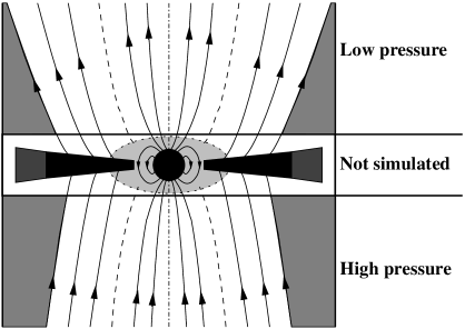
Figure 2: The northern hemisphere assumes a lower pressure, and hence a lower degree of collimation, as compared to the southern. The sketch is not in scale, the effects of this mechanism will hold at any distance wherein distinct environments are encountered. The magnetic field topology here is simple, a dipolar stellar magnetosphere is surrounded by a bipolar disk field.

In the second scenario, shown in Fig. 2, the properties of the medium along the propagation axis are assumed to affect the collimation of the jet. Specifically, the outer pressure could modify the diameter of the outflow and in turn it would determine the wind speed. This mechanism does not depend on any YSO time scale, and it could appear at any height that the jet encounters heterogeneous environment. We note that although a thermal pressure of a hot tenuous medium is used in the simulations, this could equivalently represent the pressure due to a cold dense environment, turbulence or even a large scale magnetic field. Stute et al. (Stu08 (2008)) truncated ADO solutions imposing a weaker outflow of the same type at outer radii. Here, we extend their study assuming a constant surrounding pressure instead, also with different values at each jet direction.

All our models focus on large enough scales avoiding the complicated dynamics of the star-disk interaction (e.g. Bessolaz et al. Bes08 (2008); Zanni et al. Zan09 (2009); Lovelace et al. Lov10 (2010)). Essentially, these mechanisms are included merely as boundary conditions, an approach frequently adopted in the literature of jet propagation studies (e.g. Ouyed et al. Ouy03 (2003); Fendt Fen06 (2006); Teşileanu et al. Tes09 (2009)).

Simulations are carried out to study the time evolution as well as the potential final steady states, comparing the results obtained between the two sides of the equatorial plane. We are especially looking for emerging asymmetries in the vertical velocity profiles. The resistive MHD regime is of particular interest (Čemeljić et al. Cem08 (2008)) since reconnection plays a key role, mainly at the locations where the magnetic field inverts sign. Furthermore, all cases are re-examined assuming that the flow has a strong time variable character, an effect that produces discontinuities along its axis. Note that we do not attempt to model the observed properties of the RW Aur jet, but rather to investigate in a general manner the intrinsic or extrinsic physical processes that could underlie the velocity asymmetry phenomenon.

The paper is structured as follows. Section §2 describes the jet models and provides information on the numerical setup. Section §3 presents and discusses the obtained results while section §4 reports the conclusions of this work.

2 Numerical models and setup

2.1 MHD equations

The non-dimensional resistive MHD equations written for the primitive variables are:

$$\frac{\partial\rho}{\partial t}+\nabla\cdot(\rho\@vec{V})=0\,,$$ (1)

$$\frac{\partial\@vec{V}}{\partial t}+(\@vec{V}\cdot\nabla)\@vec{V}+\frac{1}{\rho}\@vec{B}\times\@vec{J}+\frac{1}{\rho}\nabla P=-\nabla\Phi\,,$$ (2)

$$\frac{\partial P}{\partial t}+\@vec{V}\cdot\nabla P+\Gamma P\nabla\cdot\@vec{V}=(\Gamma-1)\eta\@vec{J}^{2}+\Lambda\,,$$ (3)

$$\frac{\partial\@vec{B}}{\partial t}+\nabla\times(\@vec{B}\times\@vec{V})=-\eta\nabla\times\@vec{J}\,.$$ (4)

The quantities $\rho$, $P$ and $\@vec{V}$ are the density, pressure and velocity respectively. The magnetic field $\@vec{B}$, which includes the factor $(4\pi)^{-1/2}$, satisfies the condition $\nabla\cdot\@vec{B}=0$. Moreover, the electric current is defined as $\@vec{J}=\nabla\times\@vec{B}$, and has also absorbed a factor $(4\pi)^{-1/2}$. The gravitational potential is given by $\Phi=-GM/R$, where $G$ is the gravitational constant, $M$ the mass of the central object and $R$ the spherical radius. The magnetic resistivity tensor has been assumed diagonal, with all its elements equal to the scalar quantity $\eta$. Finally, $\Lambda$ represents the volumetric energy gain/loss terms and $\Gamma=5/3$ is the ratio of the specific heats.

We adopt the axisymmetric cylindrical coordinates $(r,z)$ and we will express all quantities in code units. A code variable $U$ is converted to its physical units $U^{\prime}$ with the help of $U_{0}$, i.e. $U^{\prime}=U_{0}U$. The constants $U_{0}$ are specified such that the values of the quantities in the final configuration of the simulations match the typical values of real jets, such as observed velocities and densities. Specifically, $r_{0}=z_{0}=1.0\,\mathrm{AU}$, $\rho_{0}=2.1\cdot 10^{-18}\,\mathrm{g}\,\mathrm{cm}^{-3}$, $V_{0}=4.0\,\mathrm{km}\,\mathrm{s}^{-1}$, $P_{0}=3.3\cdot 10^{-7}\,\mathrm{dyne}\,\mathrm{cm}^{-2}$, $B_{0}=2.0\cdot 10^{-3}\,\mathrm{G}$ and $t_{0}=1.2\,\mathrm{yr}$.

2.2 Analytical solutions

The employed ADO solution, denoted with subscript D, is appropriate for describing disk winds. It is a steady state radially self-similar MHD outflow, namely, each quantity has a certain scaling along the disk radius based on the Keplerian rotation profile. Therefore, if all flow variables are known along a particular fieldline the spatial distribution of the entire solution can be reconstructed. This type of models have conical critical surfaces and consequently diverge on the axis. However, we substitute the inner region with the ASO solution, denoted with S, a meridionally self-similar jet. In this case, the critical surfaces have a spherical shape that effectively models stellar outflows. Some kind of energy input is required at the base of the wind to accelerate the plasma, but we do not treat this region because we simulate high altitudes that correspond to its super Alfvénic domain. Since the ADO solution is described by the polytropic index $\Gamma=1.05$, we specify the same value in the simulations which implies an energy source term $\Lambda=(5/3-\Gamma)P\nabla\cdot\@vec{V}$. We have verified that this does not significantly affect the dynamics (see also Matsakos et al. Tit08 (2008)). In other words, although thermal effects are thought to be crucial for the mass loading close to the disk surface (Ferreira & Casse Fer04 (2004)), we can neglect them above it where the magneto-centrifugal mechanism takes over. The adopted analytical solutions together with their parameters are presented in detail in M09.

2.3 Normalization and mixing

The two-component jet model parameters can be classified into two categories. The first one describes the relative normalization of the analytical solutions with the help of the following ratios:

$$\ell_{\mathrm{L}}=\frac{R_{*}}{r_{*}}\,,\quad\ell_{\mathrm{V}}=\frac{V_{\mathrm{S}*}}{V_{\mathrm{D}*}}\,,\quad\ell_{\mathrm{B}}=\frac{B_{\mathrm{S}*}}{B_{\mathrm{D}*}}\,,$$ (5)

where $R_{*}$ is the Alfvénic spherical radius of the ASO model, $r_{*}$ the cylindrical radius of the Alfvénic surface on a specific fieldline of the ADO solution and the star denotes the characteristic values at these locations. The subscripts L, V and B stand for length, velocity and magnetic field, respectively. We specify $\ell_{\mathrm{V}}=5.96$, such that the two solutions correspond to the same protostellar gravitational field. Following the guidelines of M09 we set $\ell_{\mathrm{L}}=0.1$. Note that due to the non-existence of a characteristic length scale in the ADO solution, the value of this parameter does not play any role in the combination of the two wind components. We also define $\ell_{\mathrm{B}}=0.01$, in order to provide comparable magnetic fields for the two outflows in the initial conditions of the numerical setup. Larger or lower values for this parameter would result in either a dominant stellar outflow and a negligible disk wind or the opposite, respectively.

The second class of parameters controls the combination of the two analytical models. In order to achieve a smoothly varying magnetic field and ensure the dominance of the protostellar magnetosphere in the central region, we follow an improved mixing process as compared to the one presented in M09. The merging depends on the magnetic flux functions $A_{\mathrm{D}}$ and $A_{\mathrm{S}}$, which label the field lines of each initial one-component solution. Once a total magnetic flux $A$ is defined, then the poloidal component of the magnetic field is given by:

$$\@vec{B}_{\mathrm{p}}=(\nabla A\times\hat{\phi})/r\,,$$ (6)

where $\hat{\phi}$ is the unit toroidal vector. However, a steep transition from one profile to the other could create artificial gradients in the flux which would be reflected in the magnetic field. As a result, $\@vec{B}$ could end up being excessively strong or even inverted across the matching surface.

Therefore, the footpoint of the fieldline that marks the transition, $A_{\mathrm{mix}}$, is chosen at a location where both $A_{\mathrm{D}}$ and $A_{\mathrm{S}}$ have roughly the same slope. Then, a first approximation of the total magnetic flux is defined: $A_{1}=A_{\mathrm{D}}+A_{\mathrm{S}}+A_{\mathrm{C}}$, where $A_{\mathrm{C}}$ is a constant that helps normalize $A_{\mathrm{D}}$ and $A_{\mathrm{S}}$. We require that the disk and stellar fields are exponentially damped in the central and outer regions respectively, which leads to an improved approximation for the magnetic flux:

$$A_{2}=\left\{1-\exp\left[-\left(\frac{A_{1}}{A_{\mathrm{mix}}}\right)^{2}\right]\right\}A_{\mathrm{D}}+\exp\left[-\left(\frac{A_{1}}{A_{\mathrm{mix}}}\right)^{2}\right]A_{\mathrm{S}}\,.$$ (7)

Finally, with the help of $A_{2}$ all two-component physical variables, $U$, are initialized using the following gaussian-type mixing function:

$$U=\left\{1-\exp\left[-\left(\frac{A_{2}}{A_{\mathrm{mix}}}\right)^{2}\right]\right\}U_{\mathrm{D}}+\exp\left[-\left(\frac{A_{2}}{A_{\mathrm{mix}}}\right)^{2}\right]U_{\mathrm{S}}\,.$$ (8)

This relation is also applied to generate the total initial two-component magnetic flux, $A$. The poloidal field is then derived from Eq. (6) and it is divergence free by definition.

Moreover, since accretion and protostellar variability are expected to introduce fluctuations in the ejection, the velocity prescribed on the bottom boundary is multiplied with the following function:

$$f_{\mathrm{S}}(r,t)=1+p\sin\left(\frac{2\pi t}{T_{\mathrm{var}}}\right)\exp\left[-\left(\frac{r}{r_{\mathrm{var}}}\right)^{2}\right]\,,$$ (9)

where $T_{\mathrm{var}}=2.5$ is the period of the pulsation and $r_{\mathrm{var}}=5$ is roughly the cylindrical radius at which the matching surface intersects the lower boundary of the computational box. The fractional variability is set to $p=0.5$ in the time variable models, in order to check the stability in the presence of strong perturbations and enhance reconnection when resistivity is included. Essentially, Eq. (9) provides a gaussian spatial distribution of a periodic velocity variability of $\sim$$3\,\mathrm{yr}$, that produces shocks and knot-like structures.

2.4 Numerical models

The anti-parallel configuration is initialized assuming a sudden inversion of the magnetic field beyond the fieldline rooted at $r_{\mathrm{inv}}=5$. In non-resistive MHD the two systems are entirely equivalent due to the invariance of the axisymmetric MHD equations under the following transformations: i) $\@vec{B}\to-\@vec{B}$, ii) $B_{\phi}\to-B_{\phi}$ and $V_{\phi}\to-V_{\phi}$. The finite values of the electric conductivity and its dependence on quantities such as $\@vec{J}$ is an unknown factor in YSO outflows. Therefore, we follow a simple approach applying a constant physical resistivity, with the value $\eta=1.0$, an approximation adequate to provide a rough estimate of how the system evolves in the presence of non-ideal effects. As explained in §3, this value can be considered small because it ensures the dominance of the advection terms over the resistive ones by several orders of magnitude throughout most parts of the computational box. However, this does not hold true on reconnection separatrices and hence its impact cannot be neglected there. Finally, we note that even in the ideal MHD cases, the finite size of the grid cells inevitably introduces artificial reconnection. We minimize its effects by increasing the resolution and we estimate its influence by comparing results of different mesh refinements.

On the other hand, the truncation of the jet for the low pressure hemisphere is initialized with the following process. We calculate the total pressure of the outflow, thermal plus magnetic, at the location $r_{\mathrm{P}}=30$ on the bottom boundary. Then, a constant pressure $P_{\mathrm{L}}$ of the same magnitude is applied on the domain beyond the limiting fieldline rooted at $r_{\mathrm{P}}$. In addition, the density is arbitrarily reduced by two orders of magnitude, whereas the velocity and magnetic fields are set to zero. Although pressure equilibrium holds at the bottom boundary, the weaker field and jet pressure at higher altitudes cannot compensate for the push of the external medium. As a result, a radial collapse is expected during the first steps of the simulation until the horizontal forces are balanced. For the jet propagating in the opposite direction, we assume another simulation case where the truncation is still at $r_{\mathrm{P}}$, but a higher outer pressure is applied with the value $P_{\mathrm{H}}=2P_{\mathrm{L}}$. Finally, we include a case where the medium has $P_{\mathrm{VH}}=6P_{\mathrm{L}}$ in order to discuss the morphology of the final steady state configuration.

Table 1: The numerical models, the name of which follows from the initials of their description.

Name	Variability	MHD	$B$ orientation	Outer $P$
NIP	Non-variable	Ideal	Parallel	-
NIA	Non-variable	Ideal	Anti-parallel	-
NRP	Non-variable	Resistive	Parallel	-
NRA	Non-variable	Resistive	Anti-parallel	-
VIP	Variable	Ideal	Parallel	-
VIA	Variable	Ideal	Anti-parallel	-
VRP	Variable	Resistive	Parallel	-
VRA	Variable	Resistive	Anti-parallel	-
NIPL	Non-variable	Ideal	Parallel	Low
NIPH	Non-variable	Ideal	Parallel	High
NIPVH	Non-variable	Ideal	Parallel	Very High
VIPL	Variable	Ideal	Parallel	Low
VIPH	Variable	Ideal	Parallel	High
VIPVH	Variable	Ideal	Parallel	Very High

Table 1 lists the fourteen two-component jet models considered, along with a brief description of their setup. In particular, models NIP and NIA focus on the effects of the parallel and anti-parallel magnetic field configuration in the ideal MHD formulation. Cases NRP and NRA include resistivity in order to understand the role of magnetic reconnection and Ohmic heating, especially in the regions where the magnetic field inverts sign. On the other hand, different values of an external pressure are imposed in models NIPL, NIPH and VIPVH to investigate the effects of distinct environments. We also consider the time-variable version of all previous cases to examine their behavior in the presence of flow fluctuations, i.e. models VIP, VIA, VRP, VRA, VIPL, VIPH and VIPVH.

2.5 Numerical setup

The simulations are performed with PLUTO, a modular shock-capturing numerical code for computational astrophysics (Mignone et al. Mig07 (2007); Mignone et al. Mig12 (2012)). Cylindrical coordinates are chosen in 2.5D and second order accuracy is specified in both time and space. All simulations adopt the TVDLF solver (Lax-Friedrichs scheme), a choice that is essential to retain stability but comes at the cost of increased numerical diffusivity. Outflow conditions are specified at the top and right boundaries, axisymmetric at the left, and all variables are kept fixed to their initial values on the bottom boundary. The size of our domain is $0\leq r\leq 100$ in the radial direction and $10\leq z\leq 310$ in the vertical. We are interested in radial distances less that $50$, but a larger box ensures that any boundary effects coming from the imposed zero derivative of $\@vec{B}$ will not influence our results (Zanni et al. Zan07 (2007)). Note that the detailed launching mechanisms of each component are not taken into account since the computational box starts from a finite height. The grid resolution is set to $500\times 1500$ and the simulations are carried out until $t_{\mathrm{stop}}=30$. We point out that the non-variable and non-pressure-confined simulations reach an exact steady state before $t=10$. In M09, we have studied the steady state of such two-component jet models in larger time scales and we have found that the configuration is time-independent to very high accuracy. The pressure-confined models require an order of magnitude larger evolution time to attain a quasi steady outcome, and hence we specify $t_{\mathrm{stop}}=300$ and a resolution of $300\times 900$ for efficiency purposes.

3 Results

As an overall remark, all non-truncated models reach steady states in an equivalent physical time of a few years. The final configuration of the disk wind remains close to the initial setup, demonstrating the stability of the ADO solution despite its significant modification. On the other hand, the hot stellar component gets compressed around the axis, which also results in an increase of the flow speed there. Even in the cases where the flow is strongly fluctuating, the two-component jet retains on average the properties of the unperturbed model. A steady shock that forms along a somewhat diagonal line at the lower part of the box is found to causally disconnect the jet launching regions from the propagation domain. Although a different mixing has been assumed, all the above features are common to the two-component jet models presented in M09, wherein a detailed discussion can be found.

3.1 Parallel/anti-parallel configurations in ideal MHD

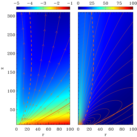
Figure 3: Logarithmic density contours along with magnetic field lines (left) and vertical velocity contours together with poloidal current lines (right) for the initial conditions of model NIP. The dashed line indicates the surface $A_{\mathrm{mix}}$ around which the mixing is assumed, and also marks the polarity reversal for the anti-parallel configurations. The thick solid line shows the separatrix beyond which a constant pressure is initially applied on the pressure-confined models. The initial setup of NIA is identical except for the opposite sign of $\@vec{B}$ and $\@vec{J}$ in the central regions.

The left panel of Fig. 3 presents the density and the magnetic field lines of the starting setup of NIP, whereas the right panel shows the distribution of the vertical velocity and the poloidal current contours. The initial configuration of NIA has an identical morphology apart from the reversal of $\@vec{B}$ and $\@vec{J}$ that takes place inside the region marked with a dashed fieldline. Essentially, this surface separates the hot stellar outflow from the cold magneto-centrifugal disk wind, that is supposed to carry most of the mass and angular momentum extracted from the system. Moreover, the pressure driven flow is faster as compared to the outer parts of the two-component model, a property associated with the normalization and the acceleration efficiency of the specific analytical solutions employed. In relation to the discussion on the mixing function, Fig. 3 demonstrates that there is a restricted choice for the location of the matching surface due to the requirement that both solutions ought to have there a magnetic field of a similar shape and magnitude. In other words, the roughly vertical field of the stellar component cannot be matched smoothly with the bent lines coming out of the disk at outer radii. Finally, the thick solid fieldline represents the truncation surface that is imposed in the simulations which study the effects of an external pressure.

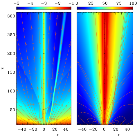
Figure 4: In the left panel, the image shows the logarithmic density and the magnetic field lines for the final steady states reached for models NIP (left hand side; parallel configuration) and NIA (right hand side; anti-parallel configuration). In the right panel, the vertical velocity distribution and electric current contours are shown for the same models. Each panel displays side by side both hemispheres of the YSO system, described in Fig. 1, in order to compare the steady states reached by the two models. Matter accumulates along the current sheet of NIA reducing the density of inner radii as well. In addition, its velocity magnitude is similar to NIP although with a more extended radial profile.

Each one of the two panels of Fig. 4 shows side by side the jet evolution of the parallel and anti-parallel configuration described in Fig. 1. In particular, the left pair shows the density and magnetic field lines of the final steady states reached by NIP (left) and NIA (right). The flipping of the field is evident in the anti-parallel case, although the general structure is maintained. From the theoretical point of view of ideal MHD, the magnetic field reversal ($\@vec{B}\to-\@vec{B}$) of a flux tube would not change the dynamics. However, the thickness of the current sheet that would form on its surface cannot be assumed zero in a physical situation.

The simulation of NIA gives a decreased value of density at inner radii and a peak along the field inversion surface. The latter feature forms simultaneously at all heights during the first steps of the simulation, and it appears more prominent in lower resolutions. In fact, numerical reconnection inevitably appears when a curved current sheet is dragged through a square cell grid. The field, and in particular the strong toroidal component that dominates the magnetic pressure, are destroyed at the interface giving rise to a perpendicular force. Matter accumulates along that surface and eventually the thermal pressure compensates the lack of the magnetic one. More accurate solvers and higher resolution would treat in a more consistent way the separatrix of the inversion of $\@vec{B}$. However, on the one hand the applied physical resistivity of the simulations presented below is well above the numerical diffusivity, and on the other, “smoothing out” effects are an important stability factor for the initial two-component magnetic field.

The right pair of Fig. 4 plots the final vertical velocity distribution and the poloidal currents for the corresponding models shown on the left. A wider radial profile of $V_{z}$ is observed in NIA as compared to NIP. Additionally, apart from the current sheet that forms in both models along the weak diagonal shock, another one also appears on the surface of the magnetic field reversal, as expected according to the previous discussion.

3.2 Parallel/anti-parallel configurations in resistive MHD

Based on the analysis of Čemeljić et al. (Cem08 (2008)) we consider the magnetic Reynolds number $R_{\mathrm{m}}=rV_{z}/\eta$ and the quantity $R_{\beta}=(P/B^{2})R_{\mathrm{m}}$, which measure the contribution of the resistive terms in the induction and energy equations, respectively.

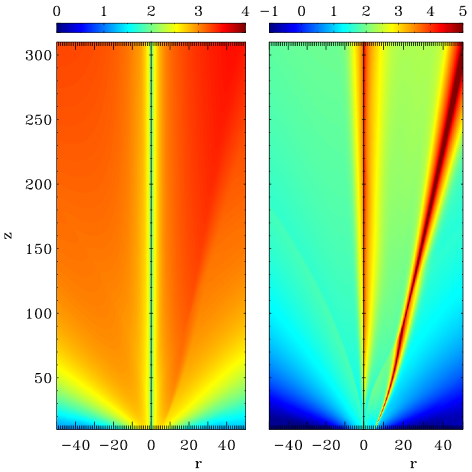
Figure 5: The logarithmic distribution of the magnetic Reynolds number $R_{\mathrm{m}}=rV_{z}/\eta$ (left panel) and $R_{\beta}=(P/B^{2})R_{\mathrm{m}}$ (right panel) for both YSO hemispheres, i.e. NRP (on the left of each pair) and NRA (on the right of each pair). Note that their definition does not include the length scale of the magnetic field reversal, but we can still observe that the resistive effects are small over most of the computational domain.

Fig. 5 displays $\log(R_{\mathrm{m}})$ (left pair) and $\log(R_{\beta})$ (right pair) for the final states of NRP (left) and NRA (right). Clearly, the magnetic Reynolds number is large in most parts of the computational domain, i.e. $R_{\mathrm{m}}\gg 1$, indicating that the diffusion of the magnetic field is not of particular importance. However, note that this definition of $R_{\mathrm{m}}$ does not take into account the magnetic field reversal whose characteristic length is much smaller than $r$ and hence the above argument excludes this region. Therefore, approximating resistivity with a small constant value is a useful approach to allow reconnection in our models without significantly affecting the validity of the ideal MHD results of the inner and outer regions.

Moreover, we observe that the condition $10<R_{\beta}<100$ holds in most parts of our domain indicating that Ohmic heating is not important either. The value of $R_{\beta}$ is also ill-defined in the anti-parallel case, since it is based on $R_{\mathrm{m}}$. Nevertheless, note that $R_{\beta}$ is large at the axis where the plasma is hot and along the matching surface that the magnetic field reconnects, due to the high values of the plasma-$\beta$ there.

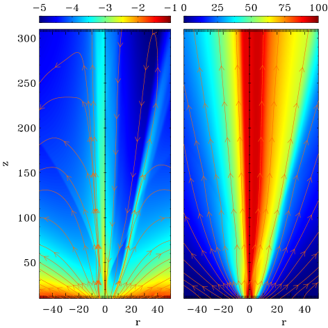
Figure 6: Side by side logarithmic density contours and magnetic field lines (left panel) for the two opposite propagating jets, i.e. NRP (on the left) and NRA (on the right). Contours of $V_{z}$ and streamlines (right panel) for the same models. Model NRA displays higher vertical velocity around the transition region as compared to NRP.

Fig. 6 shows the distribution of $\log(\rho)$ and the magnetic field lines (left pair) of the final steady states of NRP (left) and NRA (right). The right pair displays the streamlines over the contours of $V_{z}$ for the same models. Initially, the asymmetric magnetic topologies lead to distinct current distributions. Reconnection is manifested at the regions where the magnetic field inverts sign, driving a different temporal evolution between the two hemispheres. Evidently, the presence of resistive effects in the anti-parallel case results in a spatial readjustment of the velocity profile in the inner regions.

Another observed feature is the reversal of $B_{z}$ that takes place at the upper and outer domains of both NRP and NRA. This is a steady state configuration that originates from the resistive effects at the base of the outflow and a shear in the velocity profile of the flow. In particular, although the two vector fields, $\@vec{B}$ and $\@vec{V}$, are parallel at the bottom boundary, the low $R_{\mathrm{m}}$ values suggests that diffusion dominates advection at the zones right above it. As a consequence, a small angle forms between the poloidal components of $\@vec{B}$ and $\@vec{V}$ before the magnetic Reynolds number of the flow acquires high values. Shearing effects increase this angle resulting in a negative $B_{z}$ component.

Figure 7: Radial profile of $\log(\rho)$, $V_{z}$ and $\log(\rho V_{z})$ at $z=160$ for models NIP (left; dotted line), NIA (left; dashed dotted), NRP (right; dotted) and NRA (right; dashed dotted). Resistive effects are negligible for the dynamics of the parallel case, while they amplify the features observed in the ideal anti-parallel one.

Fig. 7 plots $V_{z}$ (middle) and the logarithms of $\rho$ (top), and $\rho V_{z}$ (bottom) along the radial direction at $z=160$ for models NIP (left; dotted line), NIA (left; dashed dotted line), NRP (right; dotted line) and NRA (right; dashed dotted line). From the parallel setups we deduce that the prescribed value of resistivity has a minor effect on dynamics. On the contrary, non-ideal MHD effects amplify the features of the anti-parallel configuration, namely the decrease of the density at inner radii accompanied by an increase of the speed. In addition, the peak observed in $\rho$ along the current sheet is more extended in NRA due to the physical reconnection applied. The mass flux profiles also reflect the asymmetry, despite the fact that $\rho$ and $V_{z}$ change in opposite directions. Notably, beyond the matching surface all four models demonstrate similar behaviors.

3.3 Time variable flows in parallel/anti-parallel configurations

This section investigates the previously presented models when a time variable velocity is applied on the bottom boundary, localized at the stellar component. The simulations are performed until the final time of the corresponding unperturbed cases is reached, during which several shocks propagate throughout the computational domain.

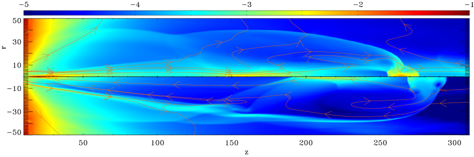
Figure 8: Logarithmic density and field lines for models VRP (top) and VRA (bottom). The two jets correspond to the two hemispheres of a YSO and are shown side by side for comparison. The shock front and matter condensations along the axis are found at different locations between the two cases. The stellar component of VRA displays a lower inner density as compared to VRP, whereas the inner part of its disk wind has higher values of $\rho$ as matter accumulated along the current sheet is blown outwards from radial shocks.

Fig. 8 compares the logarithmic density contours and the magnetic field between models VRP (top) and VRA (bottom). The shock front is slightly faster in the anti-parallel configuration and seems to have a larger radius too. High matter concentrations along the jet axis are observed at substantially different heights, i.e. $z=160$ for VRP and $z=210$ for VRA. Furthermore, higher density is also found beyond the matching fieldline of VRA suggesting that the disk wind is affected as well. In fact, the matter trapped along the current sheet is pushed radially out by the inner shocks that travel across the jet flow.

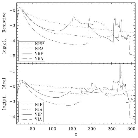
Figure 9: Logarithmic density profiles along the axis for the ideal MHD models (bottom), i.e. NIP (dotted line), NIA (dashed dotted), VIP (solid), VIA (dashed), and the resistive MHD models (top), NRP (dotted), NRA (dashed dotted), VRP (solid), VRA (dashed). The density has on average lower values in the anti-parallel cases and also peaks at different locations as compared to the parallel configuration. Especially in the presence of resistivity, decollimation drops the densities by an order of magnitude and significantly amplifies the differences between the parallel and anti-parallel models.

Fig. 9 plots the logarithm of $\rho$ along the $z$ axis for the ideal (bottom) and resistive (top) cases. Dotted/dashed-dotted lines are used for the non-variable parallel/anti-parallel configurations, and solid/dashed for the variable outflows, respectively. Density has lower overall values in the anti-parallel topology whereas flow fluctuations alter substantially its vertical profile. In particular, the high concentration regions are located at different heights as compared to the parallel setup, but without demonstrating any systematic lagging. Both features seem to become stronger when physical resistivity is included. On the one hand this implies the non-negligible role of numerical diffusivity (required for stability), and on the other, the fact that larger $\eta$ values could lead to significantly different results between the two hemispheres. Note that since emissivity is proportional to the density squared, it is expected that the above discrepancies could have a direct impact on observations. The pressure follows approximately the behavior of $\rho$ and hence it is not shown. As a result, the temperature has an almost flat profile for the ideal cases, whereas Ohmic heating slightly increases the average temperature of the resistive models, although without any distinguishable effects among them.

Figure 10: Vertical velocity and weighted average of $V_{z}$, Eq. (10), along the $z$ axis. The line style of each model follows from Fig. 9. Although the flow speed is the same among all cases, the quantity $\left<V_{z}\right>$ does demonstrate asymmetries when non-ideal MHD effects are included.

In Fig. 10, which follows the notation of Fig. 9, the vertical velocity $V_{z}$ (top) is plotted versus the $z$ direction. It was already anticipated from Fig. 7 that the parallel/anti-parallel configurations would show similar speeds. The small displacement of the shock front between the variable resistive models is evident here as well. However, having found discrepancies in the radial profile of $V_{z}$, as well as in the density distribution, we introduce the following weighted average flow velocity, that incorporates emissivity in an approximate way:

$$\left<V_{z}\right>=\frac{\int_{0}^{r_{\mathrm{max}}}\rho^{2}V_{z}\,2\pi r\,\mathrm{d}r}{\int_{0}^{r_{\mathrm{max}}}\rho^{2}\,2\pi r\,\mathrm{d}r}\,.$$ (10)

This quantity provides a better estimate for the observational implications of the simulations than $V_{z}$ alone. The integration takes place within the cylinder of radius $r_{\mathrm{max}}=30$, where $\rho$ has its highest values. Note that for altitudes $z>200$ the density peak along the current sheet is not inside the integrated domain.

The bottom panels of Fig. 10 display the vertical dependence of Eq. (10) for the corresponding models. The ideal MHD regime does not show any significant discrepancies beyond $z=200$. However, resistive cases do demonstrate velocity asymmetries both in the variable and non-variable models. The difference is of the order of $30\%$ and $20\%$, respectively, but since it depends on the specific $\eta$ value assumed, it could be much higher or even negligible in a real astrophysical situation. In addition, note that including the current sheet within the integration domain results in a slower mean speed for the anti-parallel model. This can be seen by comparing the regions $z<200$ and $z>200$. In other words, the choice of $r_{\mathrm{max}}$ also influences the absolute value of the estimated discrepancy and hence the resulting percentage should not be taken as a robust number.

Although a parametric study of $\eta$ would clarify the asymmetry dependence on finite conductivity, such a task is beyond the scopes of this work. Besides, the actual resistivity value is an unknown factor in YSOs. It suffices that even in the case of $\eta=1.0$, a small value that does not have significant effects on the parallel case, an asymmetry of $\sim$$20\mathrm{-}30\%$ is found. Nevertheless, we have performed simulations with higher and lower resistivity values that seem to agree with the above conclusions. We also note that the vertical flow velocity is constant along $z$ which indicates that there is no need to simulate larger spatial scales.

3.4 External pressure

All simulations of pressure-confined two-component jets reach quasi steady state configurations within a much larger simulation time as compared to the models presented above. This is due to the fact that the initial conditions are farther away from the equilibrium described by the ADO and ASO solutions. Moreover, all final configurations possess static knots along the flow axis as well as a wave-like cylindrical outer surface that recollimates the flow at multiple locations. The separation of these high density regions seems to increase the lower the ambient pressure applied. Notably, the variability of the inner flow does not seem to disrupt this structure, nor the shape or position of its surface. The jet models become asymptotically cylindrical, after having passed from a stage of oscillations in their radius, speed, density, and other physical parameters. Vlahakis & Tsinganos (Vla97 (1997)) have shown that, under rather general assumptions, this is a common behavior of magnetized outflows which start non-cylindrically before they reach collimation.

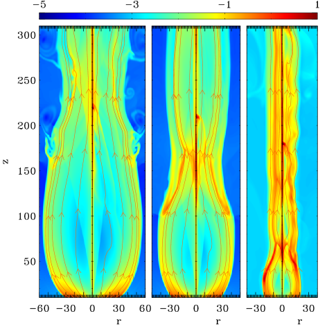
Figure 11: Logarithmic density and field lines for models NIPL, VIPL, NIPH, VIPH, NIPVH and VIPVH (from left to right). The left and middle panels correspond to the northern and southern hemispheres of Fig. 2, respectively. The right panel displays the scenario of a very high external pressure in order to visualize the oscillation of the jet’s cross section. Each panel shows the unperturbed model on the left and the time variable counterpart on the right. The outer structure as well as the condensations along the jet axis are static and unaffected by flow fluctuations.

The logarithmic density along with the field lines are shown in Fig. 11 for models NIPL, VIPL, NIPH, VIPH, NIPVH and VIPVH (from left to right). All of them have the same truncation radius, indicated in Fig. 3, but a different external pressure is imposed. Despite the pressure equilibrium holding right above the bottom boundary, the radial ram pressure of the flow expands the jet for small $z$. Eventually it becomes compensated and then recollimation occurs, compressing the flow at almost its initial diameter. At higher altitudes, the jet radius increases again and the process is repeated creating a sequence of static knots, a configuration that is stable and does not propagate with time. These features smooth out with $z$ and the jet acquires a cylindrical shape far away, as seen in model NIPVH. We have verified the stability of the static knots with simulations carried out up to $t=500$, though in a lower resolution. During time evolution, Kelvin-Helmholtz instabilities appear on the interface with the external medium, but they are gradually suppressed by the time the quasi steady state is reached.

The jet structure of NIPH seems to be a smaller copy of NIPL, and the same holds true for NIPVH with respect to NIPH. This is due to the intrinsic self-similarity property of the ADO solution, namely, all field lines have the same shape but in a different scale. Consequently, a similar outer structure is recovered in all pressure-confined cases, depending on the value of the external pressure imposed. Finally note that the mixing of the two analytical outflows introduces a length scale in the system and hence the above argument will not hold for arbitrarily small radii.

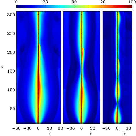
Figure 12: Vertical velocity contours for the models shown in Fig. 11, i.e. NIPL and VIPL (left panel), NIPH and VIPH (middle panel), NIPVH and VIPVH (right panel). The velocity maps follow the density distributions.

Fig. 12 displays the velocity distribution for models NIPL (left pair; left), VIPL (left pair; right), NIPH (middle pair; left), VIPH (middle pair; right), NIPVH (right pair; left) and VIPVH (right pair; right). As expected, the velocity profile reflects the static oscillations of the jet’s cross section since the mass flux is conserved. In addition, its radial dependence consists of layers of decreasing speed. Enforced time variability barely modifies the total distribution demonstrating the stability of the configuration. The small velocity observed in the outer medium is a product of the initial strong transient state in which the outflow is squeezed as the truncation surface (solid line, Fig. 3) moves upwards.

Figure 13: The quantities $\log(\rho)$, $V_{z}$ and $\left<V_{z}\right>$ (Eq. 10) along the $z$ axis, for models NIPH (dotted), NIPL (dashed dotted), VIPH (solid), VIPL (dashed). The pressure-confined jet simulations demonstrate velocity asymmetries in $V_{z}$ and become even more evident in the calculation of $\left<V_{z}\right>$.

The logarithmic density, the vertical velocity and $\left<V_{z}\right>$ are plotted along the axis in Fig. 13 for the models NIPH (dotted), NIPL (dashed dotted), VIPH (solid) and VIPL (dashed). We notice that the discrepancies are stronger in the weighted velocity, a quantity possibly relevant for observations. Moreover, $\left<V_{z}\right>$ demonstrates a difference between the cases NIPH (dotted) and VIPH (solid) which is relatively smaller as compared to the variations between the models NIPH and NIPL. This implies that the recollimation structure dominates, producing density peaks much higher than those of the enforced time variability.

Velocity asymmetries are evident in this class of simulations even without accounting emissivity. In particular, the middle plot of Fig. 13 demonstrates a $\sim$$10\%$ deviation in $V_{z}$ between the two cases. The bottom panel suggests that the observed speed of the one jet could be twice the value of the other when weighted with the square of the density, at least locally. Note that in these cases the integration is calculated for $r_{\mathrm{max}}=20$. Therefore, if a YSO outflow finds itself inside a non-uniform environment in which the pressure ratio between the two hemispheres is as low as $2$, a significant velocity asymmetry could be measured.

3.5 Mass loading

A third possible scenario is that of an increased mass loading at the base of the outflow, such as a long lived asymmetric accretion or a strong radiation source heating unevenly the disk surface. In that case, the wind density can be different above and below the equator and so will the acceleration. However, on the one hand our numerical setup is not fully appropriate to investigate this mechanism in a consistent way, and on the other, the results of such simulations did not provide adequate evidence for the formation of velocity asymmetries. Therefore, we briefly discuss this case without presenting an extensive analysis.

We have carried out simulations assuming the initial setup of NIP, but setting a two times higher density on the bottom boundary. These models allow us to examine the readjustment of the velocity profiles within a higher mass loading regime, naively assuming that all other jet properties remain the same at its base. Despite the significant modification of the boundary conditions, no considerable asymmetries have been found. Regarding the stellar component, we attribute this negative result to the fact that the outflow is already super-Alfvénic. A more consistent way to check how a high plasma mass will affect the velocity is to take into account the acceleration regions. However, this is not a straightforward task since it is not clear how the energy input required to drive the jet will change in a high mass loading regime. In addition, the much smaller characteristic time and lengths involved cannot be easily included in our comparably larger scale simulations. On the other hand, although the disk wind does include sub-Alfvénic regions, they appear at large radii of low density and speed that contribute negligibly to the velocity profile.

To sum up, the large scale two-component jet models presented in this paper, cannot fully capture the case of an asymmetric mass loading. The implicit assumption that the flow on the bottom boundary of each hemisphere has different mass but exactly the same velocity might not be valid if the acceleration mechanisms vary strongly with respect to the ejected mass. Nevertheless, we have verified that in the cases that this holds true, no substantial asymmetries are expected.

4 Summary - conclusions

In this paper we address the velocity asymmetries of YSO outflows by investigating two classes of candidate mechanisms that could possibly generate this feature.

The first class depends on the intrinsic properties of the YSO and assumes a parallel and an anti-parallel magnetic field configuration, one for each hemisphere. The application of physical reconnection results in different density and velocity distributions between the two sides, leading to observable speed discrepancies. This scenario can provide asymmetric jets coming from intrinsic physical conditions and processes, even without considering the complex dynamics of the star-disk interaction. The relative questions that arise are whether multipolar fields in the star-disk system can exist and survive for a time scale comparable to that of jet propagation, as well as what is the actual value of resistivity in YSO outflows, that could amplify or even suppress the asymmetry phenomenon.

The second class of mechanisms is based on external effects, namely when the YSO resides in a non-uniform environment. Imposing distinct outer pressures at some boundary line of the jet is found to directly affect the degree of collimation of each flow, which in turn results in significantly modified propagation speeds. This mechanism is appropriate to explain an outflow asymmetry on large time scales. In addition, static knots are found to manifest in the jet structure due to multiple recollimation locations. Their stability is robust despite the enforced flow perturbations, whereas their separation is found to be closely associated with the ambient pressure value. There is some evidence for stationary shocks in some systems (Matt & Böhm Ma03a (2003); Bonito et al. Bon11 (2011); Schneider et al. Sch11 (2011)), possibly associated with the collimation of the flow. However, shocks in protostellar jets are generally observed to propagate with the flow (Reipurth & Bally Rei01 (2001) and references therein). The fact that standing recollimation shocks, predicted in non-variable simulations with a confining pressure, are not generally observed in YSO jets implies that either the dynamical evolution of the outflow is not strongly affected by the environment or that recollimation shocks are present but undetected.

In the case of the RW Aur jet, it is not clear enough from the available observations whether the asymmetry is associated with the central engine (Woitas et al. Woi02 (2002); Hartigan & Hillenbrand Har09 (2009)) or with environmental effects (Melnikov et al. Mel09 (2009)). Both scenarios could in principle be feasible. We have arbitrarily selected the values of our parameters to explore both candidate mechanisms in a general manner without attempting to model this particular object. In order to understand the applicability of a particular model to interpret the velocity asymmetry, more detailed observations are required, as well as more advanced numerical models, including 3D geometry and radiative processes.

- (1) Aburihan, M., Fiege, J., Henriksen, R., & Lery, T. 2001, MNRAS, 326, 1217
- (2) Blandford, R. D., & Payne, D. G. 1982, MNRAS, 199, 883
- (3) Bessolaz, N., Zanni, C., Ferreira, J., Keppens, R., & Bouvier, J. 2008, A&A, 478, 155
- (4) Bonito, R., Orlando, S., Miceli, M., et al. 2011, ApJ, 737, 54
- (5) Čemeljić, M., Gracia, J., Vlahakis, N., & Tsinganos, K. 2008, MNRAS, 389, 1022
- (6) Chagelishvili, G. D., Bodo, G., & Trussoni, E. 1996, A&A, 306, 329
- (7) Coffey, D., Bacciotti, F., Woitas, J., Ray, T. P., & Eislöffel, J. 2004, ApJ, 604, 758
- (8) Daou, A. G., Johns-Krull, C. M., & Valenti, J. A. 2006, AJ, 131, 520
- (9) Delamarter, G., Frank, A., & Hartmann, L. 2000, ApJ, 530, 923
- (10) Donati, J.-F., & Landstreet, J.D. 2009, ARA&A, 47, 333
- (11) Edwards, S., Fischer, W., Hillenbrand, L., & Kwan, J. 2006, ApJ, 646, 319
- (12) Fendt, C. 2006, ApJ, 651, 272
- (13) Fendt, C. 2009, ApJ, 692, 346
- (14) Ferreira, J., & Casse, F. 2004, ApJ, 601, 139
- (15) Ferreira, J., Dougados, C., & Cabrit, S. 2006, A&A, 453, 785
- (16) Frank, A., & Noriega-Crespo, G. 1994, A&A, 290, 643
- (17) Frank, A., & Mellema, G. 1996, ApJ, 472, 684
- (18) Gracia, J., Vlahakis, N., & Tsinganos, K. 2006, MNRAS, 367, 201
- (19) Hartigan, P., & Hillenbrand, L. 2009, ApJ, 705, 1388
- (20) Königl, A. 1982, ApJ, 261, 115
- (21) Kwan, J., Edwards, S., & Fischer, W. 2007, ApJ, 657, 897
- (22) Long, M., Romanova, M. M., & Lovelace, R. V. E. 2007, MNRAS, 374, 436
- (23) Long, M., Romanova, M. M., & Lovelace, R. V. E. 2008, MNRAS, 386, 1274
- (24) Lovelace, R. V. E., Romanova, M. M., Ustyugova, G. V., & Koldoba, A. V. 2010, MNRAS, 408, 2083
- (25) Matsakos, T., Tsinganos, K., Vlahakis, N., et al. 2008, A&A, 477, 521
- (26) Matsakos, T., Massaglia, S., Trussoni, E., et al. 2009, A&A, 502, 217 (M09)
- (27) Matt, S., & Böhm K.-H. 2003, PASP, 115, 334
- (28) Matt, S., Winglee, R., & Böhm, K.-H. 2003, MNRAS, 345, 660
- (29) Matt, S., & Pudritz, R. 2005, ApJ, 632, 135
- (30) Matt, S., & Pudritz, R. 2008, ApJ, 678, 1109
- (31) Meliani, Z., Casse, F., & Sauty, C. 2006, A&A, 460, 1
- (32) Melnikov, S. Yu, Eislöffel, J., Bacciotti, F., Woitas, J., & Ray, T. P. 2009, A&A, 506, 763
- (33) Mignone, A., Bodo, G., Massaglia, S., et al. 2007, ApJS, 170, 228
- (34) Mignone, A., Zanni, C., Tzeferacos, P., et al. 2012, ApJS, 198, 7
- (35) Ouyed, R., Clarke, D., & Pudritz, R. E. 2003, ApJ, 582, 292
- (36) Perin, M. D., & Graham, J. R. 2007, ApJ, 670, 499
- (37) Reipurth, B., & Bally, J. 2001, ARA&A, 39, 403
- (38) Salmeron, R., Königl, A., & Wardle, M. 2011, MNRAS, 412, 1162
- (39) Sauty, C., & Tsinganos, K. 1994, A&A, 287, 893
- (40) Sauty, C., Trussoni, E., & Tsinganos, K. 2002, A&A, 389, 1068
- (41) Sauty, C., Meliani, Z., Lima, J. J. G., et al. 2011, A&A, 533, 46
- (42) Schneider, P. C., Günther, H. M., & Schmitt, J. H. M. M. 2011, A&A, 530, 123
- (43) Stute, M., Tsinganos, K., Vlahakis, N., Matsakos, T., & Gracia, J. 2008, A&A, 491, 339
- (44) Teşileanu, O., Massaglia, S., Mignone, A., Bodo, G., & Bacciotti, F. 2009, A&A, 507, 581
- (45) Teşileanu, O., Mignone, A., Massaglia, S., & Bacciotti, F. 2012, ApJ, 746, 96
- (46) Trussoni, E., Tsinganos, K., & Sauty, C. 1997, A&A, 325, 1099
- (47) Tzeferacos, P., Ferrari, A., Mignone, A., et al. 2009, MNRAS, 400, 820
- (48) Valenti, J. A., & Johns-Krull, C. M. 2004, Ap&SS, 292, 619
- (49) Vlahakis, N., & Tsinganos, K. 1997, MNRAS, 292, 591
- (50) Vlahakis, N., & Tsinganos, K. 1998, MNRAS, 298, 777
- (51) Vlahakis, N., Tsinganos, K., Sauty, C., & Trussoni, E. 2000, MNRAS, 318, 417
- (52) Wang, J. C. L., Sulkanen, M. E., & Lovelace R. V. E. 1992, ApJ, 390, 46
- (53) Woitas, J., Ray, T., Bacciotti, F., Davis, C., & Eislöffel, J. 2002, ApJ, 580, 336
- (54) Yang, H., Johns-Krull, C. M., & Valenti, J. A. 2007, AJ, 133, 73
- (55) Zanni, C., Ferrari, A., Rosner, R., Bodo, G., & Massaglia, S. 2007, A&A, 469, 811
- (56) Zanni, C., & Ferreira, J. 2009, A&A, 508, 1117