A novel efficient numerical solution of Poisson equation for arbitrary shapes in two dimensions

Abstract

We propose a novel efficient algorithm to solve Poisson equation in irregular two dimensional domains for electrostatics. It can handle Dirichlet, Neumann or mixed boundary problems in which the filling media can be homogeneous or inhomogeneous.

The basic idea of the new method is solve the problem in three steps: (i) First solve the equation $\nabla\cdot\mathbf{D}=\rho$. The inverse of the divergence operator in a restricted subspace is found to yield the electric flux density $\mathbf{D}$ by a fast direct solver in $O(N)$ operations. The $\mathbf{D}$ so obtained is nonunique with indeterminate divergence-free component. Then the electric field is found by $\mathbf{E}=\mathbf{D}/\epsilon$. But $\nabla\times\mathbf{E}=0$ for electrostatic field; hence, $\mathbf{E}$ is curl free and orthogonal to the divergence free space. (ii) An orthogonalization process is used to purify the electric field making it curl free and unique. (iii) Then the potential $\phi$ is obtained by solving $\nabla\phi=-\mathbf{E}$ or finding the inverse of the gradient operator in a restricted subspace by a similar fast direct solver in $O(N)$ operations.

Treatments for both Dirichlet and Neumann boundary conditions are addressed. Finally, the validation and efficiency are illustrated by several numerical examples. Through these simulations, it is observed that the computational complexity of our proposed method almost scales as $\textit{O}(N)$, where $N$ is the triangle patch number of meshes. Consequently, this new algorithm is a feasible fast Poisson solver.

Keywords: Fast Poisson solver; Loop-tree decomposition; Electrostatics

1 Introduction

The Poisson equation occurs in the analysis and modeling of many scientific and engineering problems. In electrostatics, Poisson equation arises when finding the electrostatic potential of an electric field in a region with continuously distributed charges [1]. It is often solved in micro- and nano-electronic device physics [2], as well as in electronic transport and electrochemistry problems in terms of the Poisson-Boltzmann equation [3]. In fluid dynamics, Poisson equations are solved to find the velocity potential in a steady-state potential flow of an incompressible fluid with internal sources or sinks [4]. Moreover, Poisson equation is also encountered in finding the steady-state temperature in an isotropic body with internal sources [5].

An accurate and efficient solution of Poisson equation is critical in various areas. For example, in design optimization of nanodevices where quantum effects are significant, a widely used scheme is to solve the coupled Schrödinger-Poisson system self-consistently [6, 7], in which Poisson equation is solved repeatedly, and concomitantly with the Schrödinger’s equation. As such, the computational load for solving Poisson equation is always of concern.

There are two main classes of solvers for linear systems from Poisson equation: direct and iterative. One of the direct solvers is the fast Poisson solver based on fast Fourier transform (FFT) [8]. Indeed, this method is extremely efficient when the solution regions are simple and regular geometries with regular grids, such as rectangular regions, 2-D polar and spherical geometries [9], and spherical shells [10]. Since practical problems usually involve complex geometries, there have been many research works on seeking alternative methods. The multifrontal method with nested dissection ordering [11] is the most efficient direct method that can deal with complex geometries. Its key idea relies on partitioning the domain using a nested hierarchical structure and generating the $LU$ decomposition from bottom up to minimize fill-ins. Typically, the computational complexity of the multifrontal method is of $O(N^{1.5})$ in two dimensions where $N$ is the dimension of the matrix.

The other class of solvers, the iterative ones, are more favorable when large systems are solved. A popular one is the approach based on integral equation techniques and accelerated by fast multipole method (FMM) [12, 13, 14, 15]. It can achieve $\textit{O}(N)$ complexity when the underlying Green’s function is available and amenable to factorization. Nevertheless, the underlying Green’s function is difficult to obtain unless involved problems have constant coefficient in free-space or separate geometries with simple boundary conditions.

Multigrid method is one of most effective preconditioning strategies for iterative Poisson solvers [16, 17, 18]. Although this method takes advantage of fine meshes and coarse meshes and can achieve nearly optimal efficiency in theory, it is difficult to implement in a robust fashion because it demands a set of hierarchical grids of different density, which is not convenient in many real world problems.

In this paper, we present a new efficient numerical solution of Poisson equation for arbitrary two-dimensional domain with homogeneous or inhomogeneous media. Unlike traditional Poisson solvers, where the potential is found directly, this new method solves for electric flux density $\mathbf{D}$ first. The electric flux is first approximated by the RWG basis. It uses the loop-tree decomposition of the RWG approximated vectorial electric flux which is a quasi-Helmholtz decomposition method developed in computational electromagnetics (CEM). With this technique, the electric flux is expressed as the combination of the loop space (subspace) (solenoidal or divergence free) part and the tree space (subspace) (quasi-irrotational) part. These two spaces, however, are non-orthogonal to each other, unlike the case of a pure Helmholtz decomposition.

Expanding the electric flux with two sets of basis functions: loop and tree basis functions, we can solve for the electric flux by a two-stage process: First, to find the tree-space part, a matrix system is derived from the differential equation, $\nabla\cdot\mathbf{D}=\rho$, and then solved by a fast tree direct solver with $\textit{O}(N_{t})$ complexity, where $N_{t}$ is the total number of tree basis functions. The obtained electric flux is nonunique as a divergence free component can always be added to it.

Second, the electric field $\mathbf{E}=\mathbf{D}/\epsilon$ is obtained but it is incorrect because $\mathbf{E}$ should be curl-free but the so-obtained electric field is not curl-free. It is polluted by the loop-space components. The loop-space part of $\mathbf{E}$ is purged by a projection procedure, which is iterative. Having acquired the curl-free electric field distribution, which is unique, we can readily get the potential distribution by solving $\mathbf{E}=-\nabla\phi$ by the fast tree solver as well.

In addition, we address the special treatments for Dirichlet and Neumann boundary conditions, respectively, which guarantee that the obtained solution is unique. Through numerical examples, we validate the feasibility and efficiency of the new method whose computational complexity almost scales as $\textit{O}(N)$, where $N$ is the triangle patch number of meshes.

To the best of our knowledge, this is the first time that quasi-Helmholtz decomposition techniques, e.g., loop-tree decomposition, are introduced to solve Poisson equation. This new method provides a feasible alternative for existing fast Poisson solvers. Moreover, the work about Poisson equation with Neumann boundary condition in homogeneous media has been reported in [19]. Here, not only does this paper extend the method to inhomogeneous medium cases, but it also addresses the special treatment for the Dirichlet boundary condition.

The organization of this paper is as follows. In Section 2, we introduce the basic problem definition and several relevant preliminaries. In Section 3, we present the algorithm for solving Poisson problem with Neumann boundary condition. Next, we offer a special treatment for Dirichlet boundary condition in Section 4. Finally, in Section 5, we will verify the validation and illustrate the efficiency of the new method by several numerical methods. Conclusions will be drawn in Section 6.

2 Preliminaries

2.1 Two dimensional Poisson problems

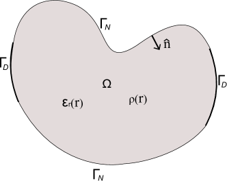
Figure 1: Schema for a typical Poisson problem.

Assume inhomogeneous dielectric materials occupying a two dimensional bounded and simply connected region, $\Omega$, with boundary $\Gamma$ and normal $\hat{\mathbf{n}}$ that points to the solution region as shown in Fig. 1. The boundary $\Gamma$ is composed of two parts: the first one, denoted by $\Gamma_{D}$, is imposed by Dirichlet boundary condition and the other part, $\Gamma_{N}$, is imposed by Neumann boundary condition.

In this paper, we are interested in solving the 2-D Poisson equation arising from electrostatic problem:

$$\begin{array}[]{ll}\nabla\cdot\epsilon_{r}(\mathbf{r})\nabla\phi(\mathbf{r})=-\rho(\mathbf{r})/\epsilon_{0}&\mbox{ for $\mathbf{r}\in\Omega$}\\ \phi(\mathbf{r})=\phi_{0}(\mathbf{r})&\mbox{ for $\mathbf{r}\in\Gamma_{D}$}\\ \frac{\partial}{\partial n}\phi(\mathbf{r})=g(\mathbf{r})&\mbox{ for $\mathbf{r}\in\Gamma_{N}$}\end{array}$$ (1)

where $\phi$ is the potential and $\rho$ describes the charge density, $\epsilon_{r}$ and $\epsilon_{0}$ are the relative permittivity and free space permittivity, respectively. Suppose that the Dirichlet boundary consists of finite $M$ distinct boundaries, $\Gamma_{D}=\bigcup_{i=1}^{M}\Gamma_{D}^{(i)}$, then a fixed potential $\phi_{0}^{(i)}$ is prescribed on the boundary $\Gamma_{D}^{(i)}$ for $i=1,2,...,M$. Moreover, to complete the description of a well-posed problem, the Neumann boundary data $g(\mathbf{r})$ must be a square integrable function over the corresponding boundary [20].

Apparently, when $\Gamma_{N}=0$, the above equation shrinks to a Dirichlet problem, which has unique solution. Similarly, it becomes a Neumann problem that is uniquely solvable (up to a constant) when $\Gamma_{D}=0$.

2.2 RWG basis

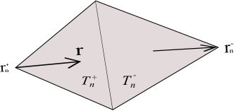
Figure 2: The geometry description of a Rao-Wilton-Glisson (RWG) function.

The Rao-Wilton-Glisson (RWG) function [21] is the most popular choice of expansion function (also called basis function) in the computational electromagnetics (CEM) community. In this paper, we use a normalized version by removing the edge length from the original definition. As shown in Fig. 2, the normalized RWG function straddles two adjacent triangles, and hence, its description requires two contiguous triangles. The expression for the expansion function describing the field on the triangle is

$$\mathbf{\Lambda}_{n}(\mathbf{r})=\left\{\begin{array}[]{cl}\pm\frac{1}{2A_{n}^{\pm}}(\mathbf{r}-\mathbf{r}_{n}^{\pm})&\mbox{ if $\mathbf{r}\in T_{n}^{\pm}$}\\ 0&\mbox{ otherwise}\end{array}\right.$$ (2)

where $\pm$ denote the respective triangles, $\mathbf{r}_{n}^{\pm}$ and $A_{n}^{\pm}$ are the vertex points and areas of the respective triangles, and $T_{n}^{\pm}$ are the supports of the respective triangles.

Apparently, RWG function is the lowest order divergence conforming function which is defined on a pair of triangles. Such basis functions can be used to expand the electric flux

$$\mathbf{D}(\mathbf{r})=\sum_{i=1}^{N}\mathbf{\Lambda}_{n}(\mathbf{r})$$ (3)

where $N$ is the total number of normalized RWG basis functions. Here, $\mathbf{D}$ is defined by

$$\mathbf{D}(\mathbf{r})=-\epsilon(\mathbf{r})\nabla\phi(\mathbf{r})$$ (4)

where

$$\epsilon(\mathbf{r})=\epsilon_{0}\epsilon_{r}(\mathbf{r})$$ (5)

is the electric permittivity.

The divergence of $\mathbf{\Lambda}_{n}$, which is proportional to the charge density associated the basis function, reads

$$\nabla\cdot\mathbf{\Lambda}_{n}(\mathbf{r})=\left\{\begin{array}[]{cl}\pm\frac{1}{A_{n}^{\pm}}&\mbox{ if $\mathbf{r}\in T_{n}^{\pm}$}\\ 0&\mbox{ otherwise}.\end{array}\right.$$ (6)

The charge density is thus constant in each triangle. The total charge associated the triangle pair, $T_{n}^{+}$ and $T_{n}^{-}$, is zero. This implies charge neutrality physically. Hence, the divergence conforming property of RWG function makes its representation of the field physical.

2.3 Helmholtz theorem and loop-tree decomposition

The well-known Helmholtz theorem [22] states that a vector field can be split into the form

$$\mathbf{f}(\mathbf{r})=\nabla\varphi+\nabla\times\mathbf{v}.$$ (7)

The first term $\nabla\varphi$ is the irrotational (curl-free) part, and the second term $\nabla\times\mathbf{v}$ is the solenoidal (divergence-free) part. Low frequency problem has been an intense research area for the last decade in the CEM community. When the frequency is low, the current naturally decomposes into a solenoidal (divergence-free) part and an irrotational (curl-free) part. These two parts are imbalanced when the frequency becomes low. Hence, there is a severe low frequency breakdwown numerical problem when solving integral equations in which RWG function is normally used. One remarkable remedy is the well known loop-tree decomposition [23, 24, 25, 26, 27, 28], in which RWG basis is decomposed into the loop basis functions that have zero divergence, and the tree basis (or star basis) functions that have nonzero divergence. This is a quasi-Helmholtz decomposition because the tree expansion functions are not curl free. For short, we call the subspace spanned by RWG basis functions the RWG space, the subspace spanned by the tree basis functions the tree space, and that spanned by loop basis functions the loop space.

Quite similar to the case of CEM, we can expand the electric flux

$$\mathbf{D}(\mathbf{r})=\mathbf{D}_{l}(\mathbf{r})+\mathbf{D}_{t}(\mathbf{r})=\sum_{i=1}^{N_{l}}l_{i}\mathbf{L}_{i}(\mathbf{r})+\sum_{i=1}^{N_{t}}t_{i}\mathbf{T}_{i}(\mathbf{r})$$ (8)

where $\mathbf{D}_{l}$ and $\mathbf{D}_{t}$ are the loop-space part and the tree space part respectively, $\mathbf{L}_{i}(\mathbf{r})$ is a loop expansion function such that $\nabla\cdot\mathbf{L}_{i}(\mathbf{r})=0$, and $\mathbf{T}_{i}(\mathbf{r})$ is a tree expansion function such that $\nabla\cdot\mathbf{T}_{i}(\mathbf{r})\neq 0$, the numbers of the loop basis functions and the tree basis functions are $N_{l}$ and $N_{t}$, respectively.

2.4 Loop basis and tree basis

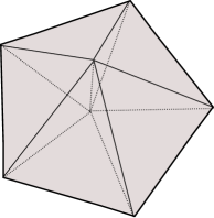
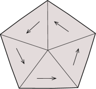
Figure 3: Linear pyramid basis function and loop basis function. Left: pyramid function. Right: loop basis function.

A loop basis function is described by the surface curl of a vector function, namely,

$$\mathbf{L}(\mathbf{r})=\nabla_{s}\times\hat{z}\,\Delta(\mathbf{r})$$ (9)

where the scalar function $\Delta(\mathbf{r})$, also referred as “solenoidal potential” [29], is the linear Lagrange or nodal interpolating basis. As shown in the left part of Fig. 3, $\Delta_{i}(\mathbf{r})$ is a piecewise linear function with support on the triangles that have a vertex at the $i$th node of the mesh, attaining a unit value at node $i$, and linearly approaching zero on all neighboring nodes. This interpolating scalar functions is also intuitively called pyramid basis functions. Moreover, the right one of Fig. 3 illustrates the loop basis function $\mathbf{L}_{i}$ associated with an interior node $i$. Within the triangles attached to node $i$, $\mathbf{L}_{i}$ has a vector direction parallel to the edge opposite to node $i$ and forms a loop around node $i$.

One the other hand, the tree basis consists of RWG functions that lie along a tree structure connecting the centroids of adjacent triangular patches. Fig. 4 shows one possible choice of the tree basis for this particular triangular mesh.

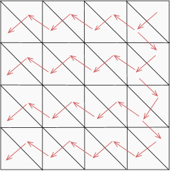
Figure 4: A possible tree basis illustration. Every arrow stands for an RWG function that is the member of tree basis.

3 Proposed method for Neumann problems

For Neumann problems, the equation in question becomes

$$\begin{array}[]{ll}\displaystyle\nabla\cdot\epsilon_{r}(\mathbf{r})\nabla\phi(\mathbf{r})=-\rho(\mathbf{r})/\epsilon_{0}&\mbox{ for $\mathbf{r}\in\Omega$}\\ \frac{\partial}{\partial n}\phi(\mathbf{r})=g(\mathbf{r})&\mbox{ for $\mathbf{r}\in\Gamma$}\end{array}$$ (10)

where $\Gamma$ includes all the boundaries of $\Omega$.

A necessary condition for the existence of a solution to this problem is that the source and boundary data satisfy the compatibility condition [30]

$$\int_{\Gamma}-\epsilon(\mathbf{r})g(\mathbf{r})d\textit{l}+\int_{\Omega}\rho(\mathbf{r})d\mathbf{r}=0.$$ (11)

For Neumann problems in homogeneous media, the basic idea of proposed method and the solution process have been reported in [19]. In this section, we extend this approach to handle more complex Poisson problems that involve inhomogeneous media.

3.1 Algorithm outline

We outline the overall solution procedures as follows:

1. Acquire the tree space part of electric flux density: By solving a matrix system resulting from $\nabla\cdot\mathbf{D}=\rho$, we first obtain the tree space part of electric flux density, $\mathbf{D}_{t}$, that corresponds to the second term on the right side of Eq. (8). Taking advantage of the fast tree solver, we can obtain $\mathbf{D}_{t}$ in $\textit{O}(N_{t})$ operations.

2. Field projection onto loop space: In order to get the first term on the right side of Eq. (8), the loop-space part $\mathbf{D}_{l}$, we need to follow up with a projection procedure. Since the electric field $\mathbf{E}$ is curl free and orthogonal to the divergence-free space, this can be achieved by projecting the electric field $\mathbf{E}$ onto the loop space and orthogonalizing it with respect to the loop space, as presented in Section 3.3. By this technique, the desired electric field will be retrieved.

3. Solution of potential: The potential distribution can be found by solving another matrix system accelerated by the fast tree solver that is of $\textit{O}(N_{t})$, in a manner similar to that of the first procedure.

3.2 Solution of $\mathbf{D}_{t}$

We start with the loop-tree decomposition of electric flux

$$\mathbf{D}(\mathbf{r})=\sum_{i=1}^{N_{l}}l_{i}\mathbf{L}_{i}(\mathbf{r})+\sum_{i=1}^{N_{t}}t_{i}\mathbf{T}_{i}(\mathbf{r})$$ (12)

where the first term of right hand side is the loop-space part, and the second one is the tree space part.

Meanwhile, from electrostatic theory, we have

$$\nabla\cdot\mathbf{D}(\mathbf{r})=\rho(\mathbf{r}).$$ (13)

The charge density $\rho(\mathbf{r})$ can be expanded in terms of pulse expansion functions [28], namely,

$$\rho(\mathbf{r})=\sum_{i=1}^{N_{p}}q_{n}P_{n}(\mathbf{r})$$ (14)

where $N_{p}$ is the number of triangle patches.

When Eqs. (12) and (14) are substituted into Eq. (13) and testing Eq. (13) with a set of pulse functions, we have a matrix system

$$\overline{\mathbf{K}}\cdot\textbf{I}_{t}=\textbf{V}_{\rho}$$ (15)

where

$$\left[\overline{\mathbf{K}}\right]_{ij}=\left\langle P_{i}(\mathbf{r}),\nabla\cdot\textbf{T}_{j}(\mathbf{r})\right\rangle$$ (16)

$$\left[\textbf{V}_{\rho}\right]_{i}=\left\langle P_{i}(\mathbf{r}),\rho(\mathbf{r})\right\rangle=q_{i}$$ (17)

and $\textbf{I}_{t}=[t_{1}\;t_{2}\;t_{3}\;\cdots\;t_{N_{t}}]^{T}$. The number of tree basis functions, $N_{t}$, is equal to $N_{p}-1$. There is one coefficient in (14) that is not needed due to the charge neutrality. In other words, the last coefficient can be derived from the front $N_{p}-1$ coefficients, i.e., $t_{N_{p}}=-\sum_{i=1}^{N_{p}-1}t_{i}$.

In the above, the inner product between two functions is defined as [31]

$$\left\langle f_{1},f_{2}\right\rangle=\int f_{1}(\mathbf{r})f_{2}(\mathbf{r})d\mathbf{r}$$ (18)

where the integral is assumed to converge. Moreover, the above matrix system is irrelevant to the loop-space part of electric flux $\textbf{D}_{l}$ because it is divergence free, i.e., $\nabla\cdot\mathbf{D}_{l}=0$.

3.2.1 Impose Neumann boundary condition

The above derivation only works for zero Neumann boundary condition, namely,

$$\frac{\partial}{\partial n}\phi(\mathbf{r})=0\mbox{ $\qquad$ for $\mathbf{r}\in\Gamma$}.$$

When the normal components of the electric field is not trivial on the boundary, we need to handle it carefully.

Physically, Eq. (11) implies that Neumann boundary condition corresponds to the 2D surface charge density introduced into the solution system. Hence, we can add extra half RWG basis functions at the boundary where non-zero Neumann boundary condition appears. The coefficients of those half RWG functions are proportional to normal electric field at corresponding boundary points.

3.2.2 Fast tree solver

The matrix system (15) can be solved with $\textit{O}(N_{t})$ operations using the fast tree solver. Its key component relies on back substitution along a tree structure (e.g., see Fig. 4). From a mathematical point of view, we can invert the matrix $\overline{\mathbf{K}}$ of Eq. (15) with linear complexity since a row permutation of the matrix is a lower triangle matrix with very few elements per row. This can be achieved with the help of topological information. We refer interested readers to Chapter 5 in [28] for details.

3.3 Loop space projection

If the media is homogeneous, both the electric flux and electric field have no loop-space or divergence-free component existing, namely, $\nabla\times\mathbf{D}=\nabla\times\mathbf{E}=0$. Hence, we can project the obtained $\mathbf{D}_{t}$ onto the loop space or divergence-free (solenoidal) space in order to remove the divergence free part to retrieve the desired field. This is because the desired electric field is orthogonal to the loop (divergence-free) space. The procedure is called divergence-free field removal as in [19].

Unfortunately, it is not the case in inhomogeneous media where the electric flux has both divergence-free and curl-free parts. It is not orthogonal to the loop space any more. However, the electric field $\mathbf{E}$ is curl free and orthogonal to the divergence-free space. Hence, we project the electric field $\mathbf{E}$ onto the divergence-free space, in order to remove its divergence-free component.

By solving the Eq. (15), coefficients $\{t_{i}\}_{i=1}^{N_{t}}$ have been obtained and known while $\{l_{i}\}_{i=1}^{N_{l}}$ are the unknowns. We can transform Eq. (12) to electric field

$$\mathbf{E}(\mathbf{r})=\sum_{i=1}^{N_{l}}l_{i}\frac{\mathbf{L}_{i}(\mathbf{r})}{\epsilon(\mathbf{r})}+\sum_{i=1}^{N_{t}}t_{i}\frac{\mathbf{T}_{i}(\mathbf{r})}{\epsilon(\mathbf{r})}.$$ (19)

Since the electric field lives in the curl free (irrotational) space, which is orthogonal to the loop space, we have

$$\left\langle\mathbf{L}_{i},\mathbf{E}\right\rangle=0.$$ (20)

Testing Eq. (19) by loop basis functions and substituting the above into it, we obtain a matrix system

$$\overline{\mathbf{G}}_{l}\cdot\mathbf{I}_{l}=\mathbf{V}_{t}$$ (21)

where

$$\left[\overline{\mathbf{G}}_{l}\right]_{ij}=\left\langle\mathbf{L}_{i}(\mathbf{r}),\frac{\mathbf{L}_{j}(\mathbf{r})}{\epsilon(\mathbf{r})}\right\rangle$$ (22)

$$\mathbf{V}_{t}=-\overline{\mathbf{R}}\cdot\mathbf{I}_{t}$$ (23)

$$\left[\overline{\mathbf{R}}\right]_{ij}=\left\langle\mathbf{L}_{i}(\mathbf{r}),\frac{\mathbf{T}_{j}(\mathbf{r})}{\epsilon(\mathbf{r})}\right\rangle$$ (24)

$\mathbf{I}_{l}=[l_{1},\;l_{2},\;l_{3},\;\cdots,\;l_{N_{l}}]^{T}$ is the unknown, and $\mathbf{I}_{t}=[l_{1},\;l_{2},\;l_{3},\;\cdots,\;l_{N_{t}}]^{T}$ is known.

Many iterative solvers could be chosen to solve Eq. (21), such as CG, Bi-CGSTAB [32] and GMRES [33, 34]. According to our experience, GMRES has the best performance if no preconditioning technique is applied. Once $\mathbf{I}_{l}$ is found, the numerically approximated curl-free $\mathbf{E}$ field is known. From it, we can derive the potential $\phi$.

3.4 Solution of potential

According to the electrostatic theory, the potential satisfies

$$-\nabla\phi(\mathbf{r})=\mathbf{E(r)}.$$ (25)

We can further expand it by a set of pulse functions

$$\phi(\mathbf{r})=\sum_{i=1}^{N_{p}}\nu_{i}P_{i}(\mathbf{r}).$$ (26)

By substituting Eqs. (19) and (26) into Eq. (25) and testing it with a set of pulse basis functions, it gives

$$\overline{\mathbf{K}}^{T}\cdot\textbf{I}_{\phi}=\textbf{V}_{\phi}$$ (27)

where

$$\left[\textbf{V}_{\phi}\right]_{i}=-\left\langle\textbf{T}_{i}(\mathbf{r})\cdot\frac{\textbf{D}(\mathbf{r})}{\epsilon(\mathbf{r})}\right\rangle$$ (28)

$$\left[\overline{\bf K}^{T}\right]_{ij}=\left\langle P_{j}(\mathbf{r}),\nabla\cdot\textbf{T}_{i}(\mathbf{r})\right\rangle=\left[\overline{\bf K}\right]_{ji}.$$ (29)

and $\textbf{I}_{\phi}=[\nu_{1}\;\nu_{2}\;\nu_{3}\;\cdots\;\nu_{N_{p}-1}]^{T}$. In the same manner as Section 3.2, there is one coefficient in (26) that is dependent on the others. Such coefficient has to be specified as a particular value before Eq. (27) is solved. This is because the solution of the Neumann problem is found up to an arbitrary constant, which corresponds to a reference potential physically. This reference potential does not affect the solution of the pertinent problem. This is also reflective of the fact that the inverse of the gradient operator is not unique.

It is interesting that the resulting matrix is just a transpose of the matrix $\overline{\mathbf{K}}$ from Section 3.2. Hence, we can solve (27) with the fast tree solver in $\textit{O}(N_{t})$ operations similar to Section 3.2.

4 Special treatment for Dirichlet boundary

Handling Dirichlet boundary conditions is of importance since Poisson problems with Dirichlet boundary conditions commonly occur in practical applications. As discussed in above section, our proposed Poisson solver works for Neumann problems. When it comes to the Dirichlet problems or mixed boundary problems, however, we need to transform the original problem to the Neumann problem to approximate it numerically.

If we consider the Poisson problem as shown in Fig. 1, then the governing equation is

$$\begin{array}[]{ll}\nabla\cdot\epsilon_{r}(\mathbf{r})\nabla\phi(\mathbf{r})=-\rho(\mathbf{r})/\epsilon_{0}&\mbox{ for $\mathbf{r}\in\Omega$}\\ \frac{\partial}{\partial n}\phi(\mathbf{r})=g(\mathbf{r})&\mbox{ for $\mathbf{r}\in\Gamma_{N}$}\\ \phi(\mathbf{r})=V_{l}&\mbox{ for $\mathbf{r}\in\Gamma_{Dl}$}\\ \phi(\mathbf{r})=V_{r}&\mbox{ for $\mathbf{r}\in\Gamma_{Dr}$}\end{array}$$ (30)

where $V_{l}$ and $V_{r}$ are potential values imposed on left and right part of Dirichlet boundary, $\Gamma_{Dl}$ and $\Gamma_{Dr}$, respectively.

At the first place, we transform the above to be the superposition of two Poisson problems with appropriate boundary conditions. The first problem (denoted by P1) is

$$\begin{array}[]{ll}\nabla\cdot\epsilon_{r}(\mathbf{r})\nabla\phi_{1}(\mathbf{r})=-\rho(\mathbf{r})/\epsilon_{0}&\mbox{ for $\mathbf{r}\in\Omega$}\\ \frac{\partial}{\partial n}\phi_{1}(\mathbf{r})=g(\mathbf{r})&\mbox{ for $\mathbf{r}\in\Gamma_{N}$}\\ \phi_{1}(\mathbf{r})=V_{l}&\mbox{ for $\mathbf{r}\in\Gamma_{Dl}$}\\ \phi_{1}(\mathbf{r})=V^{\prime}_{r}&\mbox{ for $\mathbf{r}\in\Gamma_{Dr}$}\\ \end{array}$$ (31)

where $V^{\prime}_{r}$ is a potential value arisen when we approximate this set equations.

The second one (denoted by P2) is as follows

$$\begin{array}[]{ll}\nabla\cdot\epsilon_{r}(\mathbf{r})\nabla\phi_{2}(\mathbf{r})=0&\mbox{ for $\mathbf{r}\in\Omega$}\\ \frac{\partial}{\partial n}\phi_{2}(\mathbf{r})=0&\mbox{ for $\mathbf{r}\in\Gamma_{N}$}\\ \phi_{2}(\mathbf{r})=0&\mbox{ for $\mathbf{r}\in\Gamma_{Dl}$}\\ \phi_{2}(\mathbf{r})=V_{r}-V^{\prime}_{r}&\mbox{ for $\mathbf{r}\in\Gamma_{Dr}$}.\end{array}$$ (32)

Obviously, the solution of original problem is just

$$\phi(\mathbf{r})=\phi_{1}(\mathbf{r})+\phi_{2}(\mathbf{r}).$$ (33)

Although these two sets of equations satisfy the Dirichlet boundary condition, we can resolve them by finding the solutions of two Neumann problems, as described in the following.

4.1 Solution of P1

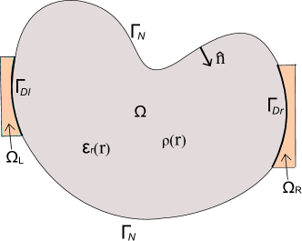
Figure 5: A schema for treatment of Dirichlet boundary conditions: Two extended regions, $\Omega_{L}$ and $\Omega_{R}$, are introduced and assumed filled with extremely high permittivity material.

From electromagnetic theory, the surface of a perfect electric conductor (PEC) or perfect magnetic conductor (PMC) serves as equipotential surface under static or quasistatic conditions. Hence, a Dirichlet boundary condition occurs when the equipotential value is known. In addition, it is known that a PEC may be regarded as a dielectric material with infinite permittivity.

Based on the above theory, a technique has been developed to surmount the difficulties arising from Dirichlet boundary conditions. Its basic scheme is illustrated in Fig. 5: Two small regions, namely, the left extended region $\Omega_{L}$ and the right extended one $\Omega_{R}$, are introduced into the solution system; both regions are filled with enormously high permittivity dielectric materials that mimic PECs to achieve equipotential surfaces. In the context of numerical implementation, we normally endow these materials with an enormously large relative permittivity, e.g., $10^{6}$.

Since the electric field inside high permittivity material becomes weak, and the electric field is related to the gradient of potential ($\mathbf{E}=-\nabla\phi$), we can reasonably assume that the boundary of extended regions, $\Gamma^{\prime}_{D}$, has homogeneous Neumann boundary condition, where

$$\Gamma^{\prime}_{D}=(\partial\Omega_{L}-\Gamma_{Dl})+(\partial\Omega_{R}-\Gamma_{Dr})$$

as illustrated in Fig. 5.

As a result, we obtain the following equation subject only to the Neumann boundary condition to resolve problem P1:

$$\begin{array}[]{ll}\nabla\cdot\epsilon_{r}(\mathbf{r})\nabla\phi_{1}(\mathbf{r})=-\rho_{1}(\mathbf{r})/\epsilon_{0}&\mbox{ for $\mathbf{r}\in\Omega$}\\ \frac{\partial}{\partial n}\phi_{1}(\mathbf{r})=0&\mbox{ for $\mathbf{r}\in\Gamma^{\prime}_{D}$}\\ \frac{\partial}{\partial n}\phi_{1}(\mathbf{r})=g(\mathbf{r})&\mbox{ for $\mathbf{r}\in\Gamma_{N}$}.\end{array}$$ (34)

It should be mentioned that, the charge distribution $\rho_{1}(\mathbf{r})$ has identical distribution as the original $\rho(\mathbf{r})$ in $\Omega$, whereas the extended regions, i.e., $\Omega_{L}$ and $\Omega_{R}$, need to be treated carefully as below.

At first, in accordance to (11), $\rho_{1}(\mathbf{r})$ must satisfy

$$\int_{\Omega_{L}+\Omega_{R}}\rho_{1}(\mathbf{r})d\mathbf{r}=\int_{\Gamma_{N}}\epsilon(\mathbf{r})g(\mathbf{r})d\textit{l}-\int_{\Omega}\rho(\mathbf{r})d\mathbf{r}=Q^{\prime},$$ (35)

where $Q^{\prime}$ is just a constant for a particular problem. It implies the quantity of charge for which the solution should compensate to guarantee charge neutrality. To this end, a simple but effective way is to allocate a line charge with the quantity of $Q^{\prime}$ inside either $\Omega_{L}$ or $\Omega_{R}$.

Next, with appropriate setting of $\rho_{1}(\mathbf{r})$ in extended regions, we can solve Eq. (34) by our new method in Section 3. It should be noted that, when solving the above equations, we must adjust the reference potential so that $\phi_{1}(\mathbf{r})$ has the value of $V_{l}$ on the left extended region $\Omega_{L}$. This can be done because the Neumann problem needs a specified a reference potential point, as discussed in Section 3.4, and high permittivity material yields an equipotential on the surface. Hence, we can adjust that reference potential for convenience. In the right extended region $\Omega_{R}$, by contrast, a floating potential $V^{\prime}_{r}$, that is not necessarily equal to $V_{r}$, will appear (we call it floating potential because this equipotential value is unknown before the solution is obtained). The arising of this floating potential does not matter for our method since we can compensate it in the following procedure.

4.2 Solution of P2

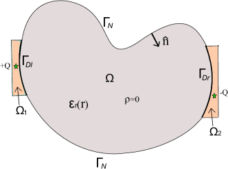
Figure 6: A schema for solving P2: Two extended regions, $\Omega_{L}$ and $\Omega_{R}$, are introduced and assumed filled with extremely high permittivity material; two line sources that have identical quantity but opposite signs are allocated in $\Omega_{L}$ and $\Omega_{R}$ respectively.

We have shown in the above section that the Dirichlet problem P1 can be solved by a Neumann problem with extended high permittivity regions. This technique can be applied to solving the second problem P2 as well. The solution of P2 is obtained by solving

$$\begin{array}[]{ll}\nabla\cdot\epsilon_{r}(\mathbf{r})\nabla\phi_{2}(\mathbf{r})=Q[\delta(\mathbf{r}-\mathbf{r}_{1})-\delta(\mathbf{r}-\mathbf{r}_{2})]&\mbox{ $\mathbf{r}\in(\Omega+\Omega_{L}+\Omega_{R})$}\\ \frac{\partial}{\partial n}\phi_{2}(\mathbf{r})=0&\mbox{ for $\mathbf{r}\in\Gamma^{\prime}_{D}$ or $\Gamma_{N}$}\end{array}$$ (36)

where $\delta(\mathbf{r})$ refers to a 2-dimensional Dirac delta function that corresponds to a line charge and $Q$ is a value relative to the potential difference $V_{r}-V_{r}^{\prime}$ between $\Omega_{L}$ and $\Omega_{R}$. Moreover, $\mathbf{r}_{1}$ is one point in $\Omega_{L}$ while $\mathbf{r}_{2}$ is another point of $\Omega_{R}$. This scheme is illustrated in Fig. 6.

A numerical difficulty, however, arises in the above equations because the value of $Q$ is not determined at this point. Fortunately, this value of $Q$ is unimportant and can be ignored in the solution process. To this end, instead of solving Eq. (36) directly, we first find the solution of another Poisson problem with unit line charge:

$$\begin{array}[]{ll}\nabla\cdot\epsilon_{r}(\mathbf{r})\nabla\tilde{\phi}_{2}(\mathbf{r})=\delta(\mathbf{r}-\mathbf{r}_{1})-\delta(\mathbf{r}-\mathbf{r}_{2}),&\mbox{ $\mathbf{r}\in(\Omega+\Omega_{L}+\Omega_{R})$}\\ \frac{\partial}{\partial n}\tilde{\phi}_{2}(\mathbf{r})=0,&\mbox{ for $\mathbf{r}\in\Gamma^{\prime}_{D}$ or $\Gamma_{N}$}.\end{array}$$ (37)

Next, having obtained the solution $\tilde{\phi}_{2}$, we can examine the potential difference between two extended regions, $\Omega_{L}$ and $\Omega_{R}$. More specifically, suppose this potential difference is $\tilde{V}_{2}$, we have

$$\phi_{2}(\mathbf{r})=\frac{V_{r}-V_{r}^{\prime}}{\tilde{V}_{2}}\tilde{\phi}_{2}(\mathbf{r}).$$ (38)

This is because for Eqs. (36) and (37) the potential difference between two ends are linearly proportional to the quantity of charge in question.

Clearly, the solution process of Eq. (37) has no difference from that of P1. In addition, since we need to solve this equation only once for a particular geometry, the computational load of this procedure is small in many applications, such as the electron transport problem in which Poisson equations are solved repeatedly.

5 Numerical results

In this section, several examples of 2-D Poisson problems will be solved to demonstrate the effectiveness of the proposed method. First, two typical 2-D Poisson problems will be simulated to show the validity and efficiency. Then, this solver will be applied to a Poisson problem that arises from a practical double-gate MOSFET electron transport simulation.

This new algorithm has been implemented in C++ and compiled with an Intel compiler. Moreover, all simulations listed below are performed on an ordinary PC with $2.66$ GHz CPU, $4$ GB memory and Windows operating system. Furthermore, in order to give a fair comparison, the same sparse matrix structure is used for both the proposed Poisson solver (denote by PPS below) and the finite element method (FEM).

5.1 Simple heterogeneous Poisson problem

First, we consider a 2-D Poisson equation in heterogeneous media as a reference problem:

$$\begin{array}[]{cl}\nabla\cdot\epsilon_{r}(x,y)\nabla\phi(x,y)=-\pi\cos(\pi x)-\pi\cos(\pi y)&\mbox{ $\qquad$ $(x,y)\in\Omega$}\end{array}$$ (39)

where $\Omega=\left[0,1\right]\times\left[0,1\right]$, and the relative permittivity

$$\epsilon_{r}=\left\{\begin{array}[]{cl}1,&x<0.5\\ 2,&x\geq 0.5.\end{array}\right.$$

For convenience, we assume that this problem has zero Neumann boundary condition and a reference potential $2/\pi$ is imposed at the origin.

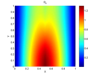
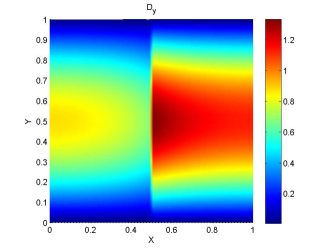
Figure 7: The electric electric flux density calculated by the proposed method. Left: $x$ component of the electric flux density $\mathbf{D}$. Right: $y$ component of the electric flux density $\mathbf{D}$.

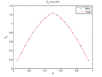
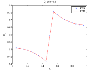
Figure 8: Comparison of the electric flux, $\mathbf{D}$, along one line between result of proposed Poisson solver (PPS) and that of FEM. Left: $x$ component of the electric flux. Right: $y$ component of the electric flux.

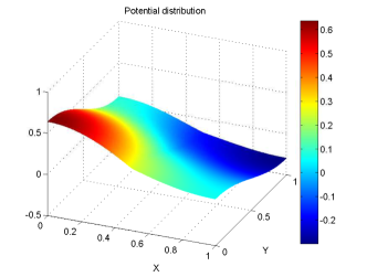
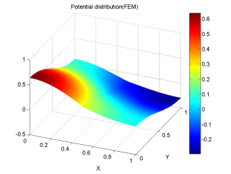
Figure 9: Calculated potential distribution. Left: the result of the proposed method. Right: the result of FEM.

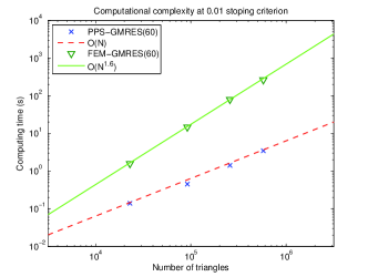
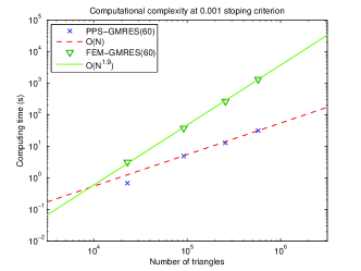
Figure 10: Computational complexity comparison between the proposed Poisson solver (PPS) and FEM method. Left: 0.01 stopping criterion. Right: 0.001 stopping criterion.

Fig. 7 shows calculated $x$- and $y$-components of electric flux density $\mathbf{D}$. Because there is discontinuity for $\epsilon_{r}$ at $x=0.5$, $y$-components, $D_{y}$, appears as an abrupt change in the middle correspondingly, which is in complete agreement with the fundamental theory of electromagnetism. Therefore, our proposed method has the capability to handle discontinuous media. In addition, further comparisons between electric fluxes obtained from proposed method and traditional finite element method are given in Fig. 8, from which we can see a good agreement at every sample points. Moreover, Fig. 9 shows calculated potential distributions, in which the result of proposed method is given in the left figure while the FEM one is given in the right figure as a reference.

To examine the computational complexity, we plot the total computing time as the mesh density increases (see Fig. 10). This computing time includes three parts: (a) the first fast-tree solution time corresponding to Section 3.2, (b) loop-space projection time corresponding to Section 3.3 and (c) the second fast tree solution time corresponding to Section 3.4. Among them, (a) and (c) can be computed expeditiously with veracious $\textit{O}(N)$ complexity which has been proved in [25], whereas (b) includes an iterative procedure that dominates the total solution time. Apparently, the iteration solution time depends on the iterative solver type and the required accuracy level. In our numerical experiment, we observe that the total solution time of our proposed method is close to $\textit{O}(N)$ complexity when GMRES solvers, without any preconditioning techniques, are applied in this problem with two different stopping criterion: $1\times 10^{-2}$ and $1\times 10^{-3}$. By contrast, as shown in plots of Fig. 10, the computational complexities of traditional FEM method are approximately of $\textit{O}(N^{1.5})$ and $\textit{O}(N^{1.9})$ at the given stopping criterion, respectively. Hence, this new proposed method demonstrates impressive efficiency compared with the FEM method.

5.2 Complex Poisson problem with Dirichlet boundary condition

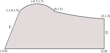
Figure 11: A two dimensional region where the Poisson problem is defined.

Next, to show the capability of handling Dirichlet boundary conditions, we simulate a general two-dimensional Poisson equation, which is

$$\begin{array}[]{cl}\nabla\cdot\epsilon_{r}(\mathbf{r})\nabla\phi(\mathbf{r})=-\delta(\mathbf{r}-\mathbf{r}^{\prime})&\mbox{ $\qquad$ for $\mathbf{r}\in\Omega$}\\ \end{array}$$ (40)

with boundary condition

$$\begin{array}[]{ll}\phi(\mathbf{r})=1.0&\mbox{ $\mathbf{r}\in\Gamma_{1}$}\\ \phi(\mathbf{r})=0.8&\mbox{ $\mathbf{r}\in\Gamma_{2}$}\\ \frac{\partial}{\partial n}\phi(\mathbf{r})=0&\mbox{ $\mathbf{r}\in$ other boundaries,}\end{array}$$

and $\mathbf{r}^{\prime}$ is the point $(-0.2,0.6)$.

Fig. 11 shows the specifications of solution region $\Omega$. This problem is excited by a line source that is located at point $\mathbf{r}^{\prime}$ with unit charge and imposed Dirichlet boundary conditions on the left and right edges.

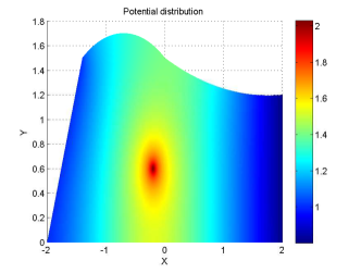
Figure 12: Potential distribution calculated from two method. Left: the proposed method. Right: FEM method.

With the technique described in Section 4, we can solve this problem by the proposed method. In our numerical experiment, the region is discretized into $133,388$ triangle patches, using the following function to approximate the line source

$$\delta(x,y)=\left\{\begin{array}[]{cl}625&|x|<0.02,|y|<0.02\\ 0&\mbox{otherwise}.\end{array}\right.$$

As for the iterative solver, GMRES with restart number $60$ is employed. Finally, the calculated potential distribution is shown in Fig. 12: The left figure shows the potential distribution calculated by our proposed method while the right one gives FEM results as the reference. It is shown that our proposed method can produce the same results as the reference one. Hence, not only Neumann boundary conditions, but also Dirichlet boundary conditions can be handled by our proposed solver competently.

To inspect the efficiency, we observe the pertinent computing resource of both the proposed method and the traditional FEM method. Both methods apply GMRES iterative solver with a restart number $60$, without any preconditioning. Table 1 lists the solution time and iteration number for both methods. As seen from this table, both iteration number and solution time of the proposed method are considerably less than that of the traditional FEM method.

Table 1: A comparison of solution times between proposed method and traditional finite element method.

	Proposed method		FEM
Stopping criteria	Iterative steps	Solution times (second)	Iterative steps	Solution times (second)
$1\times 10^{-2}$	26	0.779	31	0.889
$1\times 10^{-3}$	104	4.742	256	11.216
$1\times 10^{-4}$	295	14.446	2468	111.976
$1\times 10^{-5}$	593	28.89	4813	297.539

5.3 Application to double-gate MOSFET

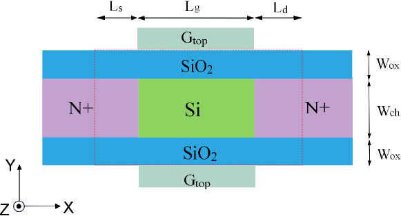
Figure 13: Two-dimensional view of the n-type double-gate silicon MOSFET.

Finally, the solver is used to simulate a multigate silicon MOSFET, as shown in Fig. 13, which is a promising candidate for the next generation nanotransistor. The structure is infinite in the $z$ direction. Gate length is denoted by $L_{g}$; source and drain extension lengths are denoted by $L_{s}$ and $L_{d}$, respectively; silicon channel thickness is $W_{ch}$; and oxide thickness is $W_{ox}$. In our simulation, the device parameters are $L_{g}=10$ nm, $L_{s}=L_{d}=4$ nm, $W_{ch}=5$ nm, and $W_{ox}=1$ nm; doping density is $N^{+}=10^{26}/m^{3}$; the relative permittivity of silicon is $11.9$; and relative permittivity of the silicon dioxide is $3.8$. Other parameters can be found in [7].

In this simulation, we find the solution of the following Poisson equation:

$$\nabla\cdot\left[\epsilon(x,y)\nabla V_{D}(x,y)\right]=q[n(x,y)-N_{d}(x,y)]$$ (41)

where $V_{D}$ is the potential to be found, $n(x,y)$ is electron density distribution given by Schrödinger solver. Here, $N_{d}$ is the doping density and $q$ is the electron charge which is equal to $1.62\times 10^{-19}$ coulombs. The simulation domain is the region enclosed by dashed line in Fig. 13. Moreover, the Dirichlet boundary condition is enforced at the gate region, whereas the floating boundary condition, i.e., the zero normal derivative, is applied at the remaining boundary.

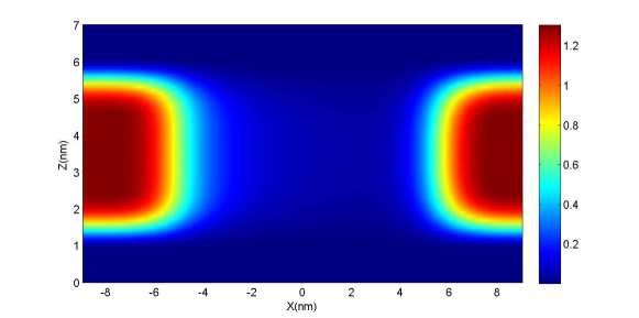
Figure 14: Two-dimensional plot of the electron density distribution.

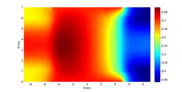
Figure 15: Two-dimensional plot of calculated potential distribution.

Fig. 14 demonstrates the electron density distribution provided from Schrödinger solver. We then use this electron density distribution as the source of Eq. (41). By our proposed method, the potential distribution is the same as the result in [7] and is shown in Fig. 15.

6 Conclusions

We have proposed and developed an efficient numerical method for solving Poisson problems. It can deal with Poisson equation with both Neumann and Dirichlet boundary conditions in a 2-D irregular region filled with homogeneous or inhomogeneous dielectrics. In this method, the electric flux is first found as opposed to traditional methods. This can be done by quasi-Helmholtz decomposition with loop-tree basis functions whose coefficients could be gained rapidly with fast solvers. Although the Dirichlet boundary condition appears as an numerical obstacle for the proposed new method, it can be overcome using special treatment: small extended regions with extremely high permittivity material are introduced to force the potential to be constant value to imitate the pertinent Dirichlet boundary conditions. Through numerical examples, it is shown that this new method can solve a general Poisson equation arising from electrostatics robustly, and has better performance than the traditional finite element method. According to our numerical experiments, it is observed that the computational complexity of this new method is close to $\textit{O}(N)$. This method is a novel fast Poisson solver that can serves as a feasible alternative to multigrid scheme for Poisson solutions.

References

- [1] J. D. Jackson, Classical Electrodynamics Third Edition, 3rd Edition, Wiley, 1998.
- [2] S. Datta, Quantum Transport: Atom to Transistor, 2nd Edition, Cambridge University Press, 2005.
- [3] F. Fogolari, A. Brigo, H. Molinari, The poisson boltzmann equation for biomolecular electrostatics: a tool for structural biology, Journal of Molecular Recognition 15 (6) (2002) 377–392. doi:10.1002/jmr.577.
- [4] H. C. Elman, D. J. Silvester, A. J. Wathen, Finite elements and fast iteratice solvers with applications in incompressible fluidd dynamics, Oxford university press, New York, 2005.
- [5] R. P. Feynman, R. B. Leighton, M. Sands, The Feynman Lectures on Physics including Feynman’s Tips on Physics: The Definitive and Extended Edition, 2nd Edition, Addison Wesley, 2005.
-
[6]
C. Cheng, J.-H. Lee, K. H. Lim, H. Z. Massoud, Q. H. Liu,
3d
quantum transport solver based on the perfectly matched layer and spectral
element methods for the simulation of semiconductor nanodevices, Journal of
Computational Physics 227 (1) (2007) 455 – 471.
doi:10.1016/j.jcp.2007.07.028.
URL http://www.sciencedirect.com/science/article/pii/S0021999107003427 - [7] J. Z. Huang, W. C. Chew, M. Tang, L. Jiang, Efficient simulation and analysis of quantum ballistic transport in nanodevices with awe, IEEE Trans. on Electron Devices 59 (2) (2012) 468–476.
- [8] G. Sköllermo, A fourier method for the numerical solution of poisson’s equations, Mathmatics of Computation 29 (131) (1975) 697–711.
- [9] M. Lai, W. Wang, Fast direct solvers for poisson equation on 2d polar and spherical geometries, Numerical Methods for Partial Differential Equations 18 (1) (2002) 56–68. doi:10.1002/num.1038.
- [10] Y.-L. Huang, J.-G. Liu, W.-C. Wang, An fft based fast poisson solver on spherical shells, Communications in Computational Physics 9 (3, SI) (2011) 649–667. doi:10.4208/cicp.060509.080609s.
- [11] T. A. Davis, I. S. Duff, An unsymmetric-pattern multifrontal method for sparse lu factorization, SIAM Journal on Matrix Analysis and Applications 18 (1) (1997) 140–158.
-
[12]
A. McKenney, L. Greengard, A. Mayo,
A
fast poisson solver for complex geometries, Journal of Computational Physics
118 (2) (1995) 348 – 355.
doi:DOI:
10.1006/jcph.1995.1104.
URL http://www.sciencedirect.com/science/article/pii/S0021999185711047 -
[13]
J. Huang, L. Greengard,
A fast direct solver
for elliptic partial differential equations on adaptively refined meshes,
SIAM J. Sci. Copmut. 21 (4) (1999) 1551–1566.
doi:DOI:10.1137/S1064827598346235.
URL http://dx.doi.org/doi/10.1137/S1064827598346235 -
[14]
F. Ethridge, L. Greengard,
A new fast-multipole
accelerated poisson solver in two dimensions, SIAM J. Sci. Copmut. 23 (3)
(2001) 741–760.
doi:DOI:10.1137/S1064827500369967.
URL http://dx.doi.org/doi/10.1137/S1064827500369967 - [15] M. H. Langston, L. Greengard, D. Zorin, A free-space adaptive fmm-based pde solver in three dimensions, Communications in Applied Mathematics and Computational Science 6 (1) (2011) 79–122.
- [16] U. Trottenberg, C. W. Oosterlee, A. Sch ller, Multigrid, Academic Press, 2001.
- [17] S. R. Fulton, P. E. Ciesielski, W. H. Schubert, Multigrid methods for elliptic problems: A review, Monthly Weather Review 14 (1986) 943–959.
- [18] L. Briggs, V. E. Henson, S. F. McCormick, A Multigrid Tutorial, SIAM, Philadelphia, 2000.
- [19] Z.-H. Ma, W. C. Chew, L. Jiang, A novel fast solver for poisson equation with the neumann boundary condition, submitted to SIAM Journal on Scientific Computing.
- [20] R. M. Brown, The mixed problem for laplace’s equation in a class of lipschitz domains, Comm. Partial Diff. Eqns. 19 (1994) 1217–1233.
- [21] S. Rao, D. Wilton, A. Glisson, Electromagnetic scattering by surfaces of arbitrary shape, Antennas and Propagation, IEEE Transactions on 30 (3) (1982) 409 – 418. doi:10.1109/TAP.1982.1142818.
- [22] J. G. V. Bladel, Electromagnetic Fields, Wiley-IEEE Press, 2007.
- [23] D. R. Wilton, A. W. Glisson, On improving the electric field integral equation at low frequencies, in: 1981 Spring URSI Radio Science Meeting Digest, Los Angeles, CA, 1981, p. 24.
- [24] J. Mautz, R. Harrington, An e-field solution for a conducting surface small or comparable to the wavelength, Antennas and Propagation, IEEE Transactions on 32 (4) (1984) 330 – 339. doi:10.1109/TAP.1984.1143316.
- [25] J.-S. Zhao, W. C. Chew, Integral equation solution of maxwell’s equations from zero frequency to microwave frequencies, Antennas and Propagation, IEEE Transactions on 48 (10) (2000) 1635 –1645. doi:10.1109/8.899680.
- [26] W. Wu, A. W. Glisson, D. Kajfez, A comparison of two low-frequency formulations for the electric field integral equation, in: Tenth Ann. Rev. Prog. Appl. Comput. Electromag., Vol. 2, 1994, pp. 484–491.
- [27] M. Burton, S. Kashyap, A study of a recent, moment-method algorithm that is accurate to very low frequencies, Appl. Comput. Electromagn. Soc. J. 10 (3) (1995) 58–68.
- [28] W. C. Chew, M. S. Tong, B. Hu, Integral Equations Methods for Electromagnetic and Elastic Waves, Morgan & Claypool, 2008.
- [29] G. Vecchi, Loop-star decomposition of basis functions in the discretization of the efie, Antennas and Propagation, IEEE Transactions on 47 (2) (1999) 339 –346. doi:10.1109/8.761074.
- [30] G. W. Hanson, A. B. Yakovlev, Operator theory for electromagnetics, Springer-Verlag, New York, 2001.
- [31] W. C. Chew, Waves and Fields in Inhomogeneous Media, IEEE Press, NJ, 1995.
- [32] H. A. van der Vorst, Bi-cgstab: A fast and smoothly converging variant of bi-cg for the solution of nonsymmetric linear systems, SIAM J. on Scientific Computing 13 (1992) 631–644.
- [33] Y. Saad, Iterative Methods for Sparse Linear Systems, 2nd Edition, Society for Industrial and Applied Mathematics, 2003.
- [34] Y. Saad, M. Schultz, Gmres: A generalized minimal residue algorithm for solving nonsymmetric linear systems, SIAM J. Sci. Stat. Comput. 7 (1986) 856–869.