Amorphous to amorphous transition in particle rafts

Abstract

Space-filling assemblies of athermal hydrophobic particles floating at an air-water interface, called particle rafts, are shown to undergo an unusual phase transition between two i.e., a low density ‘less-rigid and a high density ‘more-rigid’ amorphous states as a function of particulate number density ($\Phi$). The former is shown to be a capillary-bridged solid and the later a frictionally-coupled one. Simultaneous studies involving direct imaging as well as measuring its mechanical response to longitudinal and shear stresses show that the transition is marked by a subtle structural anomaly and a weakening of the shear response. The structural anomaly is identified from the variation of the mean coordination number, mean area of the Voronoi cells and the spatial profile of the displacement field with $\Phi$. The weakened shear response is related to local plastic instabilities caused by the depinning of the contact-line of the underlying fluid on the rough surfaces of the particles.

I Introduction

In crystalline solids in thermodynamic equilibrium, the onset of rigidity is a direct consequence of the appearance of long range positional order and the broken continuous translational symmetry. No such overarching principles are known to govern amorphous solids which are frequently out of equilibrium. For example, the onset of rigidity in athermal granular systems has been a topic of great recent interest Liu and Nagel (2010). Such studies explore the transition of a system from a state of zero rigidity (unjammed state) to that of a finite one (jammed state) Liu and Nagel (1998); Bi et al. (2011); Durian (1995); Zhang and Makse (2005). But only a few have explored further phase transitions that may exist within the jammed state of a system Zhao et al. (2011). In this paper we study the mechanical response of a rigid but amorphous particle raft to compressive (longitudinal) and shear (transverse) stresses for varying particulate number density ($\Phi$). These rafts are space-filling assemblies of athermal hydrophobic particles floating at an air-water interface and have properties common to elastic Vella et al. (2004) and granular Cicuta and Vella (2009) solids. Its mechanical response and structural reorganization reveal anomalies that are suggestive of a phase transition between two amorphous states, i.e., a low-density ‘less-rigid’ state and a high-density ‘more-rigid’ state.

II Experimental Details

II.1 Particle raft: A rigid and athermal model system

Surface tension assists hydrophobic particles which are denser than water to float on it. They deform the otherwise flat liquid surface Rapacchietta and Neumann (1977); Fournier and Galatola (2002) under gravity,  thereby generating long-range inter-particle attraction and form particulate-clusters Berhanu and Kudrolli (2010); Chan et al. (1981). The individual clusters show solid like properties,  i.e.,  they retain their shape and have a finite rigidity. However,  for small areal coverage, these clusters are sparsely distributed. Hence, at length scales comparable to the system size the collective mechanical property of the floating clusters is governed by the intervening liquid. Upon compression, i.e., increasing the areal coverage,  the individual clusters fuse to form a contiguous system spanning structure. The short-range inter-particle interactions depend on the surface roughness and wettability of the particles and are either attractive or repulsive Chan et al. (1981); Kralchevsky et al. (2001). The poly-dispersity and the athermal nature of the particles make the raft amorphous.

II.2 Experimental protocol to prepare the particle raft and its structural characterisation

The following experimental protocol is used to prepare the space filling structure of the raft.
(i) The hydrophobic (coated with FluoroPel PFC M1104V-FS from Cytonix LLC) silica particles of average diameter ($2a$) are initially sprinkled on the air-water interface in a Langmuir trough. These particles form disjoint particulate clusters (see Fig.1(a)). This state of the system is defined as a ‘ patchy’ state. For data presented in this paper,  unless otherwise mentioned,  $2a$ =0.5mm (polydispersity is 15$\%$ and density of silica is 2500 $Kg/m^{3}$).
(ii) These clusters are then brought within the interaction distance, i.e., capillary length ($L_{c}\sim 2mm$), Berhanu and Kudrolli (2010); cap   by moving the motorized Teflon barriers of the trough inwards. This constitutes the first compression cycle ($c1$). As a result of this compression the disjoint clusters coalesce to form a system-spanning quasi-two dimensional raft Kralchevsky et al. (2001); Vella et al. (2004); Cicuta and Vella (2009). The inward motion of the Teflon barriers is stopped just before the out-of-plane deformations (wrinkling) Vella et al. (2004) of the raft appear. The resulting homogeneous ‘compressed’ state of the particle raft is shown in Fig. 1(b).
(iii) The barriers are then moved outward in the first expansion cycle ($e1$) until they detach from the raft (see movie ‘MS1.avi’ in Supplementary information). Figure 1(c) shows the micrograph of the resulting relaxed,  yet rigid, state of the raft. Further cycles of compression and expansion transform the system between the ‘compressed’ and the ‘relaxed’ states.

The number density of the particles ($\Phi$) between the barriers defined as,  $\Phi=N\pi a^{2}/(L_{x}L_{y})$,  where $L_{x}$ and $L_{y}$ (=140mm) are the length and width of the raft,  respectively is chosen to be the relevant control parameter. This is guided by the literature on jamming transition Liu and Nagel (2010, 1998). The reported measurements are made in a range below the density where folds,  i.e.,  out of plane distortions Vella et al. (2004) occur (see movie ‘MS2.avi’ in Suppl. Information). The lack of distinct features beyond the third peak in the radial density pair-correlation function,  $g(r)$,  in Fig. 1(d),  illustrates that the raft remains amorphous in both the ‘compressed’ (see Fig. 1 (b)) and the ‘relaxed’ (see Fig. 1 (c)) states.

II.3 Experimental setup

The schematic of the experimental set-up is shown in Fig. 2. The system is ‘compressed’ (or expanded) by moving two motorized Teflon barriers along $x$ in steps of $0.05mm$. The system is sheared sinusoidally in the $x$-direction with a hydrophobized microscope cover-slip attached to a piezo-stage (PI-517.3CL) with a amplitude ($u_{x}^{0}$)=0.05mm and a frequency ($\nu$)=20Hz. A stainless-steel cantilever and a parallel plate capacitor is used to measure shear ($\sigma_{xy}$) and longitudinal ($\sigma_{xx}$) stresses, respectively. Details of the experimental methods and the parameters used for calculating stresses are described in Appendix A. Additionally the system is imaged under no shear for each position of the barriers. These images are then analyzed to obtain the mean coordination number ($Z$) and to generate the Voronoi diagram from which mean cell area ($A$) is calculated.

II.4 Measurement of mechanical response

The mechanical response of this system to external stresses (longitudinal and shear) is described in this paper in terms of a spatially averaged effective longitudinal and shear moduli ($K_{A}$ and $G$,  respectively) that are defined as: $K_{A}=\delta\sigma_{xx}/\delta u_{xx}$ and $G=\sigma_{xy}/u_{xy}$, where $u_{xy}=u_{x}^{0}/D$ is the shear strain,  $D=60mm$ is the distance of the cantilever from the shear-launching microscope cover-slip and $\delta u_{xx}=-\delta L_{x}/L_{x}^{0}=\delta\Phi/\Phi_{0}$ is the incremental compressive strain,  where $L_{x}^{0}$ is the length of the raft in the ‘relaxed’ (’compressed’) state for an compression (expansion) run and $\Phi_{0}$ is the density corresponding to $L_{x}^{0}$. Both $\sigma_{xx}$ and $\sigma_{xy}$ are measured with an instrumental resolution of 1 mPa. The noise observed in the data is intrinsic to the system and is a signature of finite size effect of the system. Thus the longitudinal modulus ($K_{A}$) is calculated by numerically differentiating smoothed (using a polynomial fit) $\sigma_{xx}$ with respect to $\Phi$. We note that the elastic moduli are used here as an intuitive measure of the stress-transmission defined above Hentschel et al. (2011).

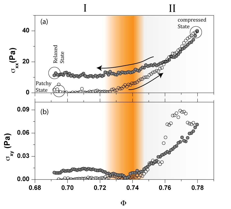
Figure 3: Variation of longitudinal stress ($\sigma_{xx}$) and shear stress ($\sigma_{xy}$) are plotted as a function of $\Phi$ in (a) and (b) respectively for $c1$ (open symbols) and $e1$ (filled symbols) cycles. The arrows in (a) shows the direction in which $\Phi$ changes. The region over which $\sigma_{xy}$ shows a softening is marked as region I. In region II,  $\sigma_{xy}$ increases rapidly. The different states of the system i.e.,  patchy,  ‘compressed’ and ‘relaxed’ are marked in the figure. The transition region separating I and II is shaded.

Figure 3 (a) and (b) show the variation of $\sigma_{xx}$ and $\sigma_{xy}$ with $\Phi$ for $c1$ (open symbols) and $e1$ (filled symbols). The first compression cycle ($c1$) starts from the patchy state (see Fig. 1 (a)) where both $\sigma_{xx}$ and $\sigma_{xy}$ are zero,  while the expansion cycle ($e1$) starts from the ‘compressed’ state (see Fig. 1 (c)). During the first compression,  system-size spanning stress-bearing networks form around $\Phi=0.74$,  marked by rapidly growing longitudinal and shear stresses. However,  during the subsequent expansion cycle towards the ’relaxed’ state ($\Phi\sim 0.69$,  as in Fig. 1(c)),  both $\sigma_{xx}$ and $\sigma_{xy}$ remain finite.

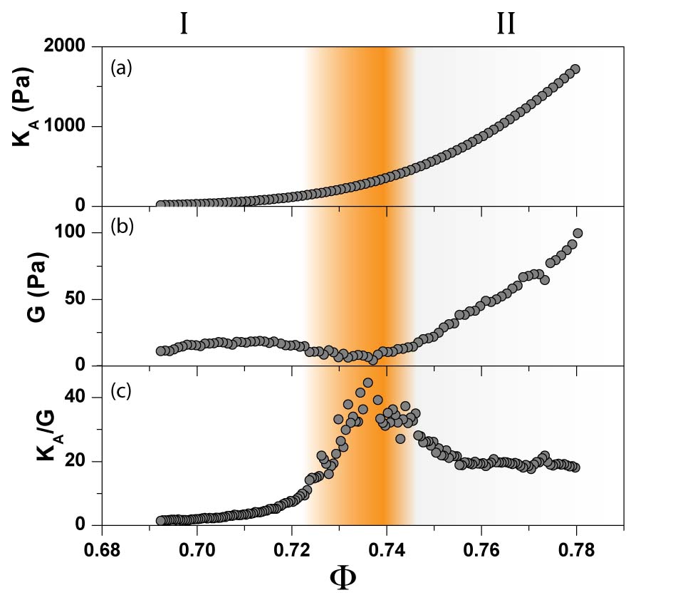
Figure 4: The variation of (a) longitudinal modulus ($K_{A}$),  (b) shear modulus ($G$),  (c) and the ratio $K_{A}/G$ as a function of $\Phi$ for the first expansion cycle.The longitudinal modulus ($K_{A}$) is calculated by numerically differentiating smoothed (using a polynomial fit) $\sigma_{xx}$ with respect to $\Phi$.

For the subsequent cycles (the first expansion onwards) the observed variation of the stresses separates into two regions: Region I for $\Phi<0.74$,  where $\sigma_{xy}$ decreases and region II for $\Phi>0.74$,  where $\sigma_{xy}$ increases rapidly with $\Phi$,  whereas $\sigma_{xx}$ increases monotonically and non-linearly with $\Phi$ in both regions. The variations in the stress transmission characteristics are illustrated through the computed $K_{A}$ and $G$,  shown in Fig. 4 (a) and (b),  respectively. The ratio, $K_{A}/G$,  shows a pronounced but inhomogeneously jagged cusp around $\Phi=0.74$ (see Fig. 4(c)) bul . The transition region is broad and shown as a shaded region in the figures.

II.5 Structural rearrangement

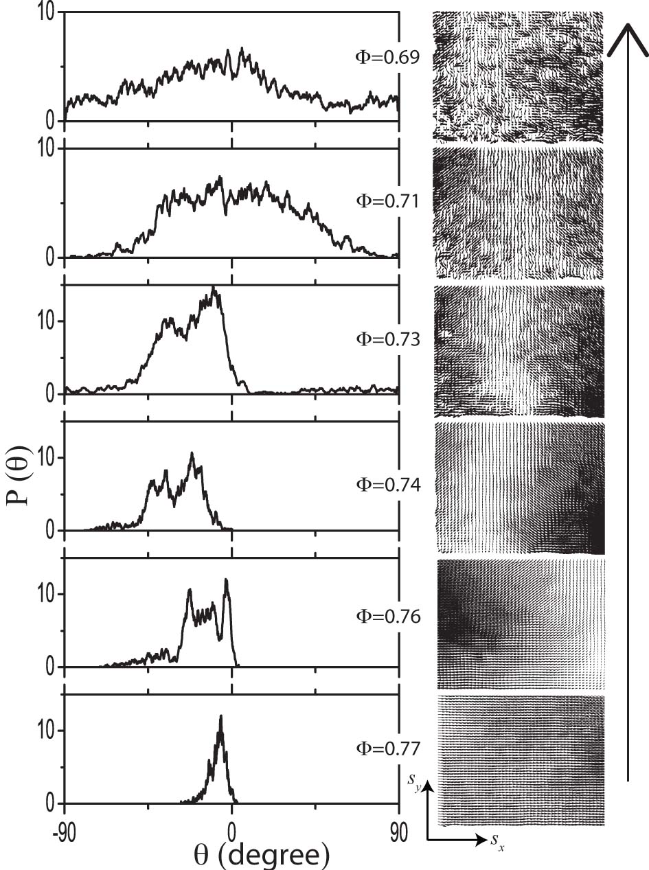
Figure 5: Displacement field of the particles and the probability distribution of angles,  $P(\theta)$ associated with the displacement vector ($\vec{s}$) measured during the first expansion cycle is shown in right and left panel respectively. Here $\theta=tan^{-1}(\frac{s_{y}}{s_{x}})$ For values of $\Phi<0.74$ the displacement field is inhomogeneous and exhibits a large number of complex cellular features (right panel). This is reflected in the broad distribution of $P(\theta)$ (left panel). However,  for values of $\Phi>0.74$,  the displacement field becomes spatially correlated over large distances and $P(\theta)$ narrows considerably. The arrow indicates the progressive sequence of $\Phi$’s, i.e, the system moves from a state of high density, i.e., $\Phi=0.77$ to a state of low density, i.e., $\Phi=0.69$.

The displacement field associated with the particles in response to the barrier movement is calculated by digitally cross-correlating an image corresponding to a specific $\Phi$ to a later one obtained after displacing the barriers by 0.25mm. The details of computing the displacement field is given in Mori and Chang . The right panel of Fig. 5 shows the typical displacement field during the first expansion cycle. The field is inhomogeneous and exhibits a large number of complex cellular features for $\Phi<0.74$. This is reflected in the broad distribution of the probability distribution function,  $P(\theta)$,  of the argument ($\theta$) associated with the displacement vectors ($\vec{s}$̂),~{}i.e.,~{}$θ=tan^-1⁡ (s_y/s_x )$\cite[cite]{\@@bibref{Authors Phrase1YearPhrase2}{ellenbroek_non-affine_2009}{\@@citephrase{(}}{\@@citephrase{)}}}shownintheleftpanelofFig.\ref{fig.2b}.However,~{}for$Φ¿0.74$thefieldbecomeshomogeneousand$ P(θ)$narrowsconsiderably.Thespatialresolutionoftheaboveimagingmethodis0.05mmanditlimitsusfromcalculatingthedisplacementfieldassociatedwiththesheardeformation.\par\par Theinhomogeneityofthedisplacementfieldatlowdensities($Φ¡0.74$)arisefrommechanicalinstabilitieswhichcanbeinterpretedasplasticeventsatthescaleoftheparticlesize(seemovie`MS3.avi^{\prime}andFig.\ref{fig.2c}).Inordertostudytheplasticityassociatedwiththemotionoftheparticles,~{}eachofthemareindividuallytracked.Representativeparticledisplacements($Δ_i$)measuredfromthe`relaxed^{\prime}stateisplottedasafunctionof$σ_xx$inFig.\ref{fig.2c}(a)forthesecondcompression(c2)cycle.Thejaggednessofthegraph,i.e.,suddenjumpsin$Δ_i${}^{\prime}s,isassociatedwithplasticity.Ameasureofthetotalnumberofplasticeventsassociatedwiththestresscyclingisobtainedfromthehysteresisofthecumulativestrainparameter$(λ),=∑Δ_i /L_x^0$,wherethesummationiscarriedoutoveralltheparticles.Figure\ref{fig.2c}(b)showsthevariationof$λ$with$σ_xx$forsuccessivecompression(opensymbols)andexpansion(filledsymbols)cycles.\par\par\par Theimagesoftheraftatvarious$Φ${}^{\prime}sareusedtofurtherexplorepossiblestructuralsignaturesofthetransition.Figure\ref{fig.3c}(a)showsanincreaseinthemeancoordinationnumber$Z$($=N ∫_2a^2a+ϵ 2 πlg(l)dl$),~{}where$ϵ$ischosentomatchthefirstpeakin$g(r)$asafunctionof$Φ$.ThecorrespondingvariationoftheVoronoicellarea$A$normalizedwiththeparticlearea($πa^2$),analternativemeasureofthelocalstructureandcompactivity\cite[cite]{\@@bibref{Authors Phrase1YearPhrase2}{katgert_jamming_2010}{\@@citephrase{(}}{\@@citephrase{)}}},isplottedinFig.\ref{fig.3c}(b).Both$Z$and$¡A¿/πa^2$varieslinearlywith$Φ$inregionI,buthoweverstarttodeviatefromtheinitialslope(shownbytheextrapolateddottedline)inthetransitionregion.Itsuggeststhatthemeasuredweakeningoftheshearmodulusisaccompaniedbystructuralreorganizationsatthelengthscaleofnearestneighborsthroughoutthesystem.\par\par\par\par$

III Discussion of results

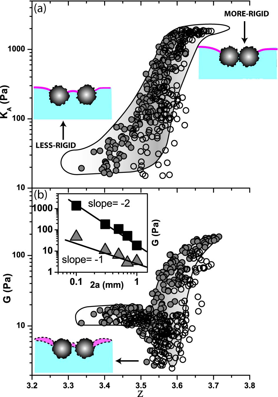
Figure 8: Variation of (a) $K_{A}$ and (b) $G$ as a function of $Z$. The filled symbols correspond to $e1$ while the open ones correspond to $c2$. The shaded regions indicate the spread in the data. The ‘less-rigid’ (schematically shown as a capillary bridged interaction in (a)) and ‘more-rigid’ states (schematically shown as a friction dominated interaction in (a)) are marked in the figure. The inverted cusp in $G$ versus $Z$ corresponds to the slipping of the contact line (schematically shown in (b) with a greater width of a sliding contact line). The inset of (b) shows the variation of $G$ of the ‘less-rigid’ (triangles) and ‘more-rigid’ (square) states of the raft as a function of particle diameter ($2a$). The solid lines passing through the data show $a^{-1}$ and $a^{-2}$ variation of $G$ for the ‘less-rigid’ and ‘more-rigid’ states,  respectively.

The choice of an order parameter in a disordered system is usually not unique and is often subjective Torquato et al. (2000). In our experiments we find the mean coordination number $Z$ is a sensitive parameter to describe the transition. The dependence of $K_{A}$ and $G$ on $Z$ is shown in Fig. 8 (a) and (b) respectively for $e1$ and $c2$. The system exhibits two terminal states,  (i) ‘less-rigid’ state ($K_{A}\sim 20$Pa and $G\sim 10$ Pa) and (ii) a ‘more-rigid’ state ($K_{A}\sim 2000$Pa and $G\sim 200$Pa). The transition from one state to the other is marked by decrease in $G$ around $Z\sim 3.6$,  although,  $K_{A}$ changes monotonically with increasing $Z$. Hence, the anomaly observed is in the variation of the shear compliance, i.e., $1/G$, reminiscent of the behavior of the magnetic susceptibility at a spin glass transition in disordered magnets Binder (1986).

The cusp in $K_{A}/G$ (see Fig. 4 (c)) is a robust feature of this transition. This is a signature of the difference in the density dependence of $K_{A}$ and $G$,  reminiscent of, but distinct from,  the power-law divergence observed in simulations of the jamming transition in frictionless granular materials Liu and Nagel (2010). However,  one must emphasize that the phenomenology observed here is far from the original definition of athermal jamming for which only hard core interaction is considered and where the transition is between rigid and non-rigid states. In the conventional sense the ’relaxed’ state of the system is already in a jammed state. The observations should be viewed as a transition between two jammed states whose differences are discussed below.

III.1 Microscopic mechanism associated with the transition

In order to understand the microscopic mechanism associated with the transition,  we investigated the dependence of $G$ on the particle size (see inset of Fig. 8 (b)). For the ‘less-rigid’ state (filled triangles),  $G\propto a^{-1}$. This is consistent with a capillary bridging mechanism ($G\sim\gamma/a$,  where $\gamma$ is the surface tension of the liquid) through the pinned contact lines of the liquid on the particles Kralchevsky et al. (2001); Vella et al. (2004). In the ‘more-rigid’ state the contact friction dominates the inter-particle interaction. The measured shear modulus ($G$) scales with the number density of contacts,  which is proportional to the number density of particles,  i.e.,  $G\propto N/(L_{x}L_{y})\sim\Phi/a^{2}$. It assumes that the roughness scale is independent of the particle size. Since this happens over a narrow range of $\Phi$,  one obtains $G\propto a^{-2}$ as in conventional elasticity in a quasi-2D system Chaikin and Lubensky (2000). We hence conclude that regions I and II represent a capillary-bridged solid and a frictional solid,  respectively.

III.2 Time dependent effects and stress cycling in the particle raft

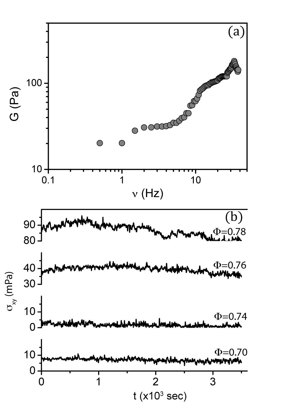
Figure 9: (a) Frequency dependence of $G$ measured at $\Phi=0.77$. (b) The time dependence (creep effect)of $\sigma_{xy}$ is shown for different $\Phi$’s.

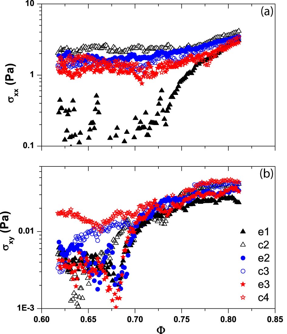
Figure 10: The figure shows the variation of $\sigma_{xx}$ and$\sigma_{xy}$ for various compression (open symbols) and expansion (filled symbols) cycles as a function of $\Phi$ for particles of diameter 1 mm. The sequence of expansion and compression are as follows,  first compression (data not shown for reasons discussed in the main text) : first expansion ($e1$: filled triangles),  second compression ($c2$: open triangles),  second expansion ($e2$: filled circles), third compression ($c3$: open circles), third expansion ($e3$: filled stars),  fourth compression ($c4$: open stars). The repeated compression-expansion cycles result in annealing of the raft and thus later cycles show a reduced but finite hysteresis.

The structural relaxation time of the particle raft,  $\tau=12\pi\eta a^{3}/mv^{2}\sim 1000s$,  where $m=0.2\mu g$ and $v=50\mu m/s$ are the mass and velocity of a single particle respectively and $\eta=1mPas$ is the viscosity of the liquid. In calculating the relaxation time,  we assume that the effective temperature of the system ($T_{eff}$) is related to the kinetic energy of the particle,  i.e.,  $T_{eff}=mv^{2}/2K_{B}$,  where $K_{B}$ is the Boltzmann’s constant. The system thus takes a long time to reach its equilibrium state. This would mean that the system would typically find itself in a kinetically arrested state and would show a dependence on the history of the paths via which a given state of the system is reached. Indeed, measurements above 1 mHz probes a frequency-dependent rigidity of the material as shown in Fig. 9(a) for $\Phi=0.77$. Moreover,  creep effects (time-dependence) in $\sigma_{xy}$ are more pronounced in region II than in region I,  as shown in Fig. 9 (b). Interestingly,  the stress allows the ‘more-rigid’ frictional solid to explore various metastable states and hence the system shows a marked ‘creep’,  i.e. a temporal variation,  in $\sigma_{xy}$. This is absent for the ‘less-rigid’ capillary solid suggesting that it is closer to a deeper metastable minimum. Strong history dependence is also seen in the variation of $\sigma_{xx}$ and $\sigma_{xy}$ measured for subsequent compression and expansion cycles which broadly follow the trend (see fig. 3) but with greatly reduced hysteresis (see Fig. 10, the data shown in the figure is for particles whose diameter is 1mm),  analogous to residual densification observed in amorphous materials Loerting et al. (2009).

IV Conclusion

We have shown that a rigid particle raft can undergo a phase transition from a ‘less-rigid’ low density state to a ‘more-rigid’ high density state as a function of particulate number density. The transition is marked by a weakening of the shear modulus. The measured shear modulus which distinguishes the two states of the system,  i.e.,  ‘less-rigid’ and ‘more-rigid’,  arises from the restoring force of pinned contact lines in the former case and from particle contacts through a frictional coupling in the latter. The weakening of the shear modulus observed in the crossover region is thus attributable to a reduction of restoring force arising from plastic events caused by the mechanical instabilities and the associated depinning of the contact lines Bourne et al. (1986); Coppersmith (1990).

Although the results presented in the present paper are specific to particle rafts,  the weakening of the shear response and local reorganization seen in the present experiment,  have also been observed in network glasses Thorpe and Duxbury (1999); Poole et al. (1997). We hope that the present experiment will provide some insight into the complex phenomenon of pressure induced phase transitions in amorphous solids Pham et al. (2002); Mishima et al. (1985); Poole et al. (1995); Sun et al. (2011); Loerting et al. (2009); Mishima and Stanley (1998).

The authors thank M. Bandi, M. Cates, N. Menon, L. Mahadevan, S. R. Nagel and A. Yethiraj for helpful discussions.

Appendix A Experimental set-up

The schematic of the experimental set-up is shown in Fig. 2. Hydrophobic silica particles are sprinkled on the air-water interface in a Langmuir trough (300mm x 145mm x 25mm) made of Teflon. These particles coalesce and form disjoint (patchy) clusters. The two motorized Teflon barriers of the trough are used to fuse these clusters into a homogeneous ‘compressed’ or ’relaxed’ state by moving the barriers inward or outward in $x$-direction respectively. The system is illuminated uniformly from the bottom using an LCD monitor through a glass window sealed in the trough and a camera above records the image in the $(x-y)$ plane at each barrier step ($=0.05mm$). The system is sheared in the $x$-direction by moving a hydrophobic cover-slip (60mm x 24mm x 0.15mm) sinusoidally $u_{x}=u^{0}_{x}{\rm cos}(2\pi\upsilon t)$,  where $u^{0}_{x}=0.05mm$ and frequency $\upsilon=20Hz$,  connected to a three-axis piezo-stage (PI-517.3CL). A stainless steel cantilever is kept at $D=60mm$ in the $y$-direction from the shear launching cover-slip as marked by (i) and shown at the left-bottom of the Fig. 2 with dimensions mentioned. The hydrophobic cover-slips attached to piezo stage and the cantilever makes contact with the particles at the air-water interface. The shear stress (${\sigma}_{xy}$) is measured from the lateral displacement of the cantilever. The displacement is sensed by a fiber optic-based displacement sensor (MTI-2000 FOTONIC) from the interference of light that is reflected from the mirror glued on the cantilever at a distance of $25mm$ from the fixed support. The output of the displacement sensor is fed to a lock-in amplifier (SR830). A parallel plate capacitor,  used as a force-sensor,  is marked by (ii) and also shown with dimensions in the right-bottom of Fig. 2. It is made of $0.2\ mm$ thick flexible polymeric sheet and kept at a distance of $30mm$ from the cantilever in the $y$-direction. The metal electrodes are glued at the bottom of the two plates of the force-sensor with a separation of 3mm and are immersed in water. A capacitance-bridge (1615-A General Radio) is used to detect the change in the plate separation during compression (or expansion) from the lateral deflection of the individual capacitor plates. The output of the capacitance-bridge is fed to another lock-in amplifier (SR830) which drives the bridge at 100KHz. The stresses,  shear (${\sigma}_{xy}$) and longitudinal ($\sigma_{xx}$),  are calculated using “bending-of-a-beam” formula using lateral displacement of the cantilever in the former case and the plate deflection in the latter. The formula used in general is given by: the stress $\sigma=6REI/x^{2}_{0}(3l_{0}-x_{0})\alpha$ Landau et al. (1986) where $R$ is the lateral displacement,  $E$ is Young’s modulus,  $I=bh^{3}/12$ is the second moment of area ($b$ and $h$ are width and thickness of the detecting object,  respectively),  $l_{0}$ is the length of the object,  $x_{0}$ is point of detection from the fixed end and $\alpha$ is an effective area of contact with the particles. All these parameters used in the calculation of stress’ are tabulated in table 1 for the cantilever and the parallel plate force sensor.

	length ($l_{0}$) (mm)	width ($b$) (mm)	thickness ($h$) (mm)	Young’s modulus ($E$) (GPa)	point of detection ($x_{0}$) (mm)	effective area ($\alpha$) (mm2)
Cantilever	90	13	0.13	200	25	30
Parallel plate force-sensor	60	25.4	0.2	2	60	12.7

Table 1: Parameters used in the calculation of $\sigma_{xx}$ and $\sigma_{xy}$ for the cantilever and the parallel plate force sensor

Figure 1: Micrographs of hydrophobized silica particles at the air-water interface in the form of (a) disjoint clusters (patchy state) and (b) a homogeneous ‘compressed’ state of the raft in presence and (c) absence (’relaxed’ state) of longitudinal stress. The scale bars, 10mm. (d) The left (right) panel shows the plot of the radial density pair correlation function,  $g(r)$,  of the ‘relaxed’ (‘compressed’) state of the system.

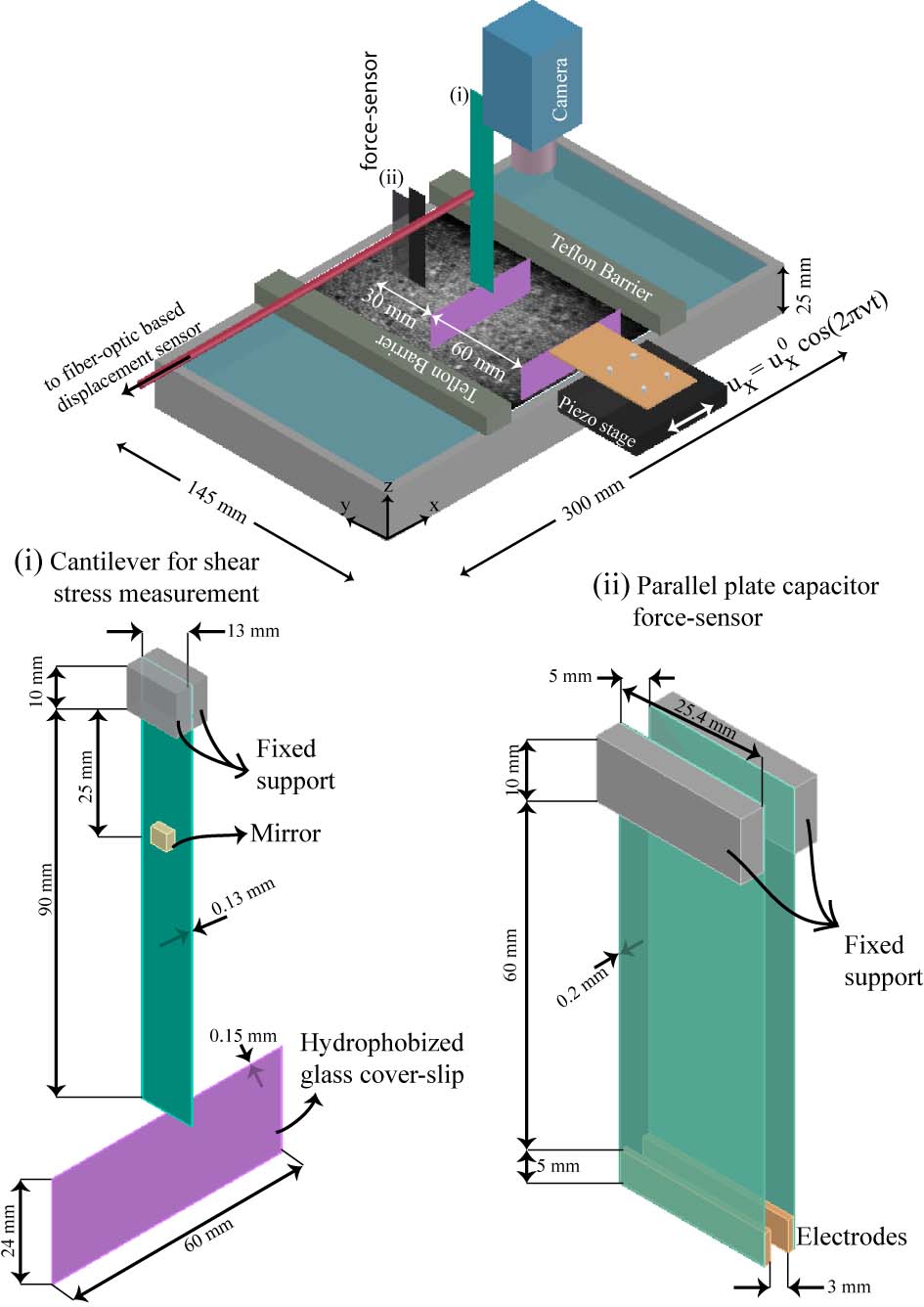
Figure 2: Experimental setup: hydrophobized microscope cover-slip attached to a piezo-stage oscillates along $x$ producing a sinusoidal shear deformation. The cantilever with an attached microscope cover-slip,  placed along $y$ at a distance ($D$)=60mm away from the piezo-stage measures the shear stress ($\sigma_{xy}$). A parallel-plate capacitor,  marked as the force-sensor,  is used to measure the longitudinal stress ($\sigma_{xx})$.

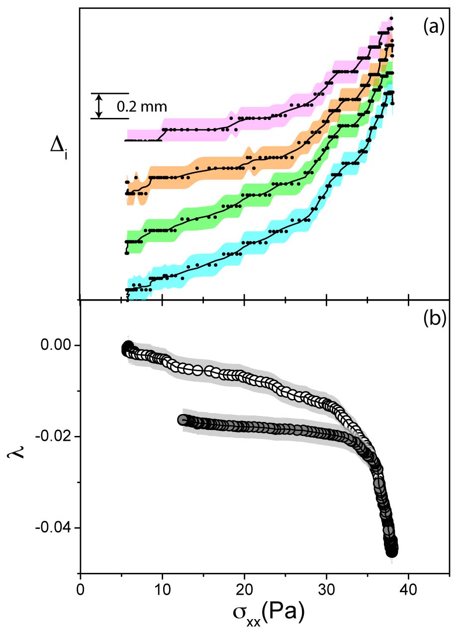
Figure 6: (a)Typical displacement curves of a few particles ($\Delta_{i}$),  measured from its position in the ‘relaxed’ state as a function of $\sigma_{xx}$. For visual clarity the curves are shifted vertically. The corresponding scale bar of the displacement is shown in the figure. The data is plotted for a compression cycle. (b) The variation of the cumulative strain ( $\lambda=\sum\Delta_{i}/L_{x}^{0}$, where the summation is over all the particles) with $\sigma_{xx}$ for successive compression (open symbols) and expansion (filled symbols) cycles. The uncertainty in the measurement of $\Delta_{i}$ and $\lambda$ is shown by the accompanying band.

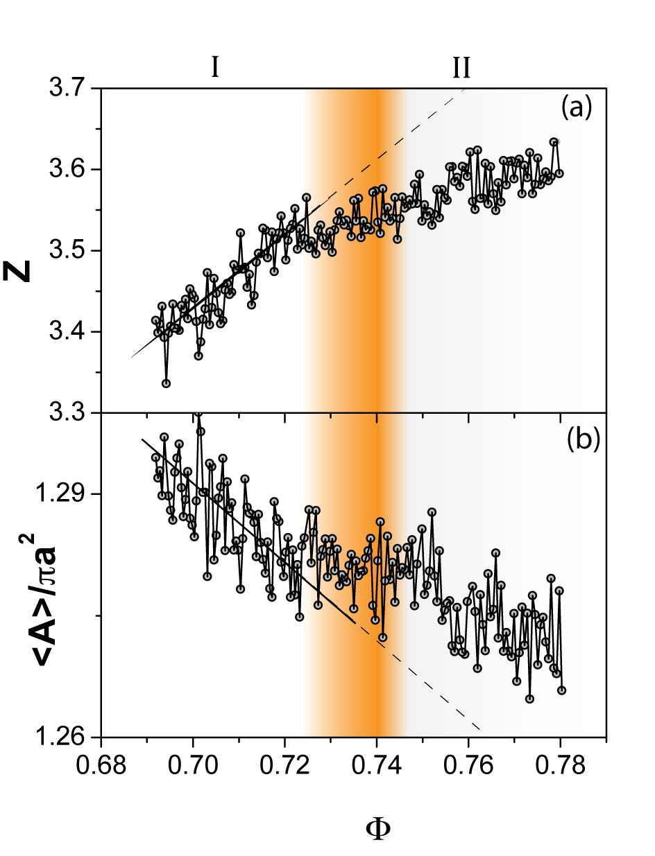
Figure 7: The variation of (a) the mean coordination number $Z$ and (b) the mean Voronoi cell area $A$ normalized with the particle’s area ($\pi a^{2}$) as a function of $\Phi$. The solid lines show their linear variation in region I. The dotted lines which are a linear extrapolation of initial variation highlights the later deviation of the graphs. The data presented here is for $e1$.

References

- Liu and Nagel (2010) A. J. Liu and S. R. Nagel, Annual Review of Condensed Matter Physics 1, 347 (2010).
- Liu and Nagel (1998) A. J. Liu and S. R. Nagel, Nature 396, 21 (1998).
- Bi et al. (2011) D. Bi, J. Zhang, B. Chakraborty, and R. P. Behringer, Nature 480, 355 (2011).
- Durian (1995) D. Durian, Physical Review Letters 75, 4780 (1995).
- Zhang and Makse (2005) H. Zhang and H. Makse, Physical Review E 72 (2005).
- Zhao et al. (2011) C. Zhao, K. Tian, and N. Xu, Physical Review Letters 106 (2011).
- Vella et al. (2004) D. Vella, P. Aussillous, and L. Mahadevan, Europhysics Letters 68, 212 (2004).
- Cicuta and Vella (2009) P. Cicuta and D. Vella, Physical Review Letters 102, 138302 (2009).
- Rapacchietta and Neumann (1977) A. V. Rapacchietta and A. Neumann, Journal of Colloid and Interface Science 59, 555 (1977).
- Fournier and Galatola (2002) J. Fournier and P. Galatola, Physical Review E 65, 031601 (2002).
- Berhanu and Kudrolli (2010) M. Berhanu and A. Kudrolli, Physical Review Letters 105, 098002 (2010).
- Chan et al. (1981) D. Chan, J. Henry jr., and L. White, Journal of Colloid and Interface Science 79, 410 (1981).
- Kralchevsky et al. (2001) P. A. Kralchevsky, N. D. Denkov, and K. D. Danov, Langmuir 17, 7694 (2001).
- (14) , where , and are the surface tension of water, density of water and acceleration due to gravity respectively.
- Hentschel et al. (2011) H. G. E. Hentschel, S. Karmakar, E. Lerner, and I. Procaccia, Physical Review E 83, 061101 (2011).
- (16) In continuum elasticity, the bulk modulus ; here, , thus .
- (17) N. Mori and K. Chang, Introduction to MPIV, URL http://www.oceanwave.jp/softwares/mpiv/,2003.
- Ellenbroek et al. (2009) W. G. Ellenbroek, Z. Zeravcic, W. van Saarloos, and M. van Hecke, Europhysics Letters 87, 34004 (2009).
- Katgert and van Hecke (2010) G. Katgert and M. van Hecke, Europhysics Letters 92, 34002 (2010).
- Torquato et al. (2000) S. Torquato, T. Truskett, and P. Debenedetti, Physical Review Letters 84, 2064 (2000).
- Binder (1986) K. Binder, Reviews of Modern Physics 58, 801 (1986).
- Chaikin and Lubensky (2000) P. M. Chaikin and T. C. Lubensky, Principles of Condensed Matter Physics (Cambridge University Press, 2000), .
- Loerting et al. (2009) T. Loerting, V. V. Brazhkin, and T. Morishita, in Advances in Chemical Physics, Volume 143, edited by S. A. Rice (John Wiley & Sons, Inc., 2009), pp. 29–82.
- Bourne et al. (1986) L. C. Bourne, M. S. Sherwin, and A. Zettl, Physical Review Letters 56, 1952 (1986).
- Coppersmith (1990) S. N. Coppersmith, Physical Review Letters 65, 1044 (1990).
- Thorpe and Duxbury (1999) M. F. Thorpe and P. M. Duxbury, Rigidity theory and applications: edited by M.F. Thorpe and P.M. Duxbury (Springer, 1999).
- Poole et al. (1997) P. H. Poole, T. Grande, C. A. Angell, and P. F. McMillan, Science 275, 322 (1997).
- Pham et al. (2002) K. N. Pham, A. M. Puertas, J. Bergenholtz, S. U. Egelhaaf, A. Moussaı̈d, P. N. Pusey, A. B. Schofield, M. E. Cates, M. Fuchs, and W. C. K. Poon, Science 296, 104 (2002).
- Mishima et al. (1985) O. Mishima, L. D. Calvert, and E. Whalley, Nature 314, 76 (1985).
- Poole et al. (1995) P. H. Poole, T. Grande, F. Sciortino, H. Stanley, and C. Angell, Computational Materials Science 4, 373 (1995).
- Sun et al. (2011) Z. Sun, J. Zhou, Y. Pan, Z. Song, H.-K. Mao, and R. Ahuja, Proceedings of the National Academy of Sciences 108, 10410 (2011).
- Mishima and Stanley (1998) O. Mishima and H. E. Stanley, Nature 396, 329 (1998).
- Landau et al. (1986) L. D. Landau, L. P. Pitaevskii, E. Lifshitz, and A. M. Kosevich, Theory of Elasticity, Third Edition: Volume 7 (Butterworth-Heinemann, 1986), 3rd ed.