Excitation of emission lines by fluorescence and recombination in IC418

Abstract

We compare calculated intensities of lines of C ii, N i, N ii  O i and O ii with a published deep spectroscopic survey of IC 418. Our calculations use a self–consistent nebular model and a synthetic spectrum of the central star atmosphere to take into account line excitation by continuum fluorescence and electron recombination. We found that the N ii spectrum of s, p and most d states is excited by fluorescence due to the low excitation conditions of the nebula. Many C ii and O ii lines have significant amounts of excitation by fluorescence. Recombination excites all the lines from f and g states and most O ii lines. In the neutral–ionized boundary the N i quartet and O i triplet dipole allowed lines are excited by fluorescence, while the quintet O i lines are excited by recombination. Electron excitation produces the forbidden optical lines of O i  and continuum fluorescence enhances the N i forbidden line intensities. Lines excited by fluorescence of light below the Lyman limit thus suggest a new diagnostic to explore the inner boundary of the photodissociation region of the nebula.

1 Introduction

With an apparent simple geometry the low excitation planetary nebula IC 418 lends itself to simpler models with fewer assumptions on its structure and kinematics than are generally necessary to reproduce observations of planetary nebulae (PNe). A recent deep spectroscopic survey of this object by Sharpee et al. (2003) (hereafter SWBH) identified several hundred lines in IC 418 from which Sharpee, Baldwin & Williams (Sharpee et al.2004) (hereafter SBW) derived ionic abundances for CNONe ions relative to H. Many dipole–allowed line intensities from those ions in that survey cannot be explained by the recombination theory with the same abundances derived from collisionally excited lines (CELs). The intensities of recombination lines are often used to measure ionic abundances because they depend more weakly on temperature and density than CELs. Abundances derived from recombination lines, however, are usually higher than those derived from CELs in the Orion nebula (Esteban et al., 1998; Baldwin et al., 2000; Esteban et al., 2004; Mesa–Delgado, Esteban, & García–Rojas, Mesa–Delgado et al.2008), many H ii regions (García–Rojas & Esteban, 2007), and planetary nebulæ (Liu et al., 1995, 2001b; Luo, Liu & Barlow, Luo et al.2001; Liu et al., 2006; Tsamis et al., 2008; García–Rojas, Peña M. & Peimbert, García–Rojas et al.2009; Otsuka et al., 2009). Williams et al. (2008) showed that CELs probably give the correct abundances because the values derived from CELs are consistent with those derived from UV absorption lines in a sample of four PNe. The discrepancies of less than a factor of 2 found by SBW in IC 418 between abundances from CELs and dipole–allowed lines are smaller than in other objects. Nevertheless it is important to ensure that the intensities of the dipole–allowed lines are not enhanced by additional excitation mechanisms besides recombination whenever they are used in temperature or density diagnostics (Fang, Storey & Liu, Fang et al.2011) (hereafter FSL) or abundance determinations.

The usual procedure to determine a species X abundance directly from optical line intensities is to measure the ratio of the intensity of a line emitted by the species with respect to the $\rm H\beta$ intensity and assume that the ratio of column densities producing the lines is equal to the abundance. Specifically, the abundance X/H is taken from the equation

$${I(\lambda)\over I(\mbox{$\rm H\beta$})}={\int\epsilon(\lambda)\,dV\over\int\epsilon(\mbox{$\rm H\beta$})\,dV}={\langle\epsilon(\lambda)\rangle\over\langle\epsilon(\mbox{$\rm H\beta$})\rangle}{\rm X\over H}$$ (1)

where $I(\lambda)/I(\mbox{$\rm H\beta$})$ is the ratio of intensities corrected for reddening, $\epsilon(\lambda)$ and $\epsilon(\mbox{$\rm H\beta$})$ are the emissivities of a line emitted by X and of $\rm H\beta$ respectively, both are integrated over some volume fraction of the nebula covered by the aperture, and $\langle\epsilon\rangle$ means some kind of average of the emissivities over that volume fraction. Averaged emissivities over the volume within the solid angle of the aperture imply the adoption of average values for the temperature, density and filling factors.

An alternative procedure to determine chemical abundances in a nebula is to propose mutually consistent models of the nebula and the atmosphere of the exciting star or stars. The stellar parameters, chemical abundances and density profile of the nebula are inputs to a photoionization model, and their values are fixed by matching the predicted line intensities to the observations. The variation of stellar and nebular parameters of the model can be constrained by direct observations of the star and nebula to reduce the degeneracy of different parameters giving similar matches to the observed line intensities. Morisset & Georgiev (2009) (hereafter MG) showed that a consistent stellar energy distribution (SED) of the central star of IC 418 and a photoionization model give an impressive agreement of predictions and measured intensities of CELs and many recombination lines within observational errors. However most dipole–allowed lines in the SWBH survey were not included in the model by MG, and some of the ones that were included show observed intensities much larger than their predicted values because the MG calculations did not include fluorescence excitation.

In this work we add fluorescence excitation of permitted lines to a photoionization model and a SED similar to the ones used by MG, and compare the results with all lines observed by SWBH that have probable identifications as dipole–allowed lines of C ii, N i, N ii, O i, and O ii and optical forbidden lines of N i and O i. Continuum fluorescence of starlight was suggested as a mechanism to excite permitted lines in ionized nebulae by Seaton (1968) and Grandi (1975, 1976). Escalante and Morisset (2005) (hereafter EM) showed that fluorescence in Orion dominates the intensities of N ii permitted lines. The low excitation level of IC 418 and the resemblance of its ionization degree to that of the Orion nebula noted by Torres–Peimbert, Peimbert & Daltabuit (Torres–Peimbert et al.1980) suggest that a similar fluorescence mechanism may occur in both objects.

2 Line emissivities

In our previous work (EM) we found that the rate of continuum fluorescence excitation typically depends on the absorption of photons in several resonant transitions, also called pumping transitions, to quantum states of moderate excitation. Excitation by recombination on the other hand involves the capture of free electrons into a much larger number of excited states. In the fluorescence and recombination mechanisms subsequent transitions to lower states produce the optical lines observed in ionized regions although many lines in the UV and IR are also emitted.

Our calculation of quantum state populations is based on the cascade matrix formalism described in detail by EM. In that formalism excited states are populated by recombinations and by transitions from the ground and metastable states. The contribution of recombinations to the population of a state $j$ is given by the effective recombination coefficient of the state, $\alpha^{\rm eff}_{j}$. The effective fluorescence coefficient defined by EM, $\beta^{\rm eff}_{gj}$, gives the contribution of pumping transitions from the ground and metastable states to excited states that produce decays ending in state $j$. Both coefficients can be calculated in terms of the cascade matrix of Seaton (1959). The emissivity of a line for a transition from state $j$ to $i$ with a branching ratio $P_{ji}$ and frequency $\nu$ at a point in the nebula is

$$\epsilon_{ji}=h\nu P_{ji}(n_{e}n^{+}\mbox{$\alpha^{\rm eff}_{j}$}+\sum_{g}n_{g}\mbox{$\beta^{\rm eff}_{gj}$})$$ (2)

where $n_{e}$ is the electron density, $n^{+}$ is the density of the ion before recombination, and $n_{g}$ is the population density of the ground or metastable state of the recombined ion or atom. The branching ratio $P_{ji}=A_{ji}/A_{j}$, where $A_{ji}$ is the Einstein coefficient for transition from states $j$ to $i$, and $A_{j}$ is the total decay rate of the upper state $j$. The line effective recombination coefficient is defined as:

$$\mbox{$\alpha^{\rm eff}_{ji}$}=P_{ji}\mbox{$\alpha^{\rm eff}_{j}$}$$ (3)

It is assumed that the ion density $n^{+}$ can be calculated from the ionization balance condition, and the ground and metastable state populations can be calculated from the balance of collisional and radiative transitions with the aid of a nebular photoionization model.

The cascade matrix formalism assumes that every transition from the continuum or from the ground or metastable state to a higher–energy state is followed by transitions to lower–energy states, and that metastable states are not significantly affected by those transitions. Those are valid assumptions at the temperatures and densities of a photoionized nebula because collisional excitation and deexcitation with electrons control the population of metastable states, but fluorescence can compete with collisions with electrons and atoms in the colder interface of the neutral and ionized part of a nebula. Bautista (1999) proposed that the forbidden lines of atomic N are excited by fluorescence and collisions with electrons and atoms in Orion. Because the collisional excitation of metastable states violates the assumption of downward transitions in the calculation of the cascade matrix, the population densities of the metastable and ground states, $n_{j}$ and $n_{k}$, must be solved for from equations of the type:

$$n_{j}\sum_{i\neq j}(A_{ji}+C_{ji})=\sum_{k\neq j}n_{k}(A_{kj}+C_{kj}+\beta^{\rm eff}_{kj})$$ (4)

where $A_{ji}=0$ if state $i$ is energetically higher than $j$, and $C_{ji}$ is the collisional excitation or deexcitation rate from states $j$ to $i$. The summations comprise all the metastable and ground states, except state $j$. The system of equations (4) is non–linear because the effective fluorescence rates depend on the optical depth of transitions from the ground and metastable states to excited states (see equations [2] through [7] of EM). We found that the system (4) can be solved iteratively by updating the optical depths across the nebula, and then using matrix inversion to solve for the populations $n_{j}$ at each point in the nebula in each iteration. The five–state inversion formulae by Kafatos & Lynch (1990) can be easily modified to include the fluorescence rates in equation (4). The emissivity of a forbidden line is then

$$\epsilon_{ji}^{\rm f}=h\nu A_{ji}n_{j}$$ (5)

Effective recombination coefficients depend on temperature and more weakly on density. They have been tabulated with their radiative and dielectronic parts for spectroscopic terms of astrophysically important ions in the literature. We assume that $\alpha^{\rm eff}_{j}$ for an individual fine structure state of a given term is proportional to the relative weight of the state $(2J+1)/\sum_{i}(2J_{i}+1)$. This is a good approximation for direct recombinations from the continuum. Nevertheless it is worth noticing that $\alpha^{\rm eff}_{j}$ adds the contribution of a large number of cascading bound–bound transitions after the free-bound transition, and probabilities of fine structure transitions are not proportional to relative weights. To date only the calculation of effective recombination coefficients of $\rm N^{+}$ by FSL has considered the fine structure splitting of quantum states.

In the calculation of $\beta^{\rm eff}_{gj}$ we split quantum states in their fine structure components either assuming the LS or LK angular momentum coupling schemes as appropriate or using published intermediate coupling calculations when available. The fine structure of states can be important in fluorescence calculations because quantum selection rules can selectively pump certain states.

The calculation of $\beta^{\rm eff}_{gj}$ involves a large number of quantum states that can be reached by downward transitions following an absorption from the ground or a metastable state. Metastable states and some core–excited states of the form $\rm 2s2p^{m+1}$ can build up a significant population under low density conditions because of their low transition probabilities to the ground state. The population densities, $n_{g}$, in equation (2) include all the fine structure states of the ground and metastable terms. Optical lines involving core–excited configurations have often been attributed to low temperature dielectronic recombination (Nussbaumer & Storey, 1981), but radiative recombination or fluorescence followed by two–electron transitions can also produce excited–core configurations. EM found that it is important to take into account spin forbidden transitions and core excited configurations in the calculation of $\beta^{\rm eff}_{gj}$.

3 Atomic data

We used the compilation in the NIST Atomic Spectra Database (Ralchenko, Kramida & Reader, Ralchenko et al.2008) to classify quantum states and store the observed energies and probabilities for some transitions. However we relied substantially on more recent and complete calculations of probabilities from other authors. Systematic variations among different atomic databases have small effects in the cascade matrix in most cases because the calculation depends on branching ratios.

3.1 $\rm C^{+}$

This ion has the simplest structure. The ground core term produces a doublet manifold of excited states $\rm 2s^{2}(^{2}S)\ nl\ ^{2}L$. Consequently free–bound transitions tend to concentrate in fewer states, and give rise to more intense lines from states with higher quantum numbers. The excited cores $\rm 2s2p$, and $\rm 2p^{2}$ produce quartet and doublet manifolds. We used the populations of the fine structure states of terms $\rm 2s^{2}2p\ ^{2}P^{o}$ and $\rm 2s2p^{2}\ {}^{4}P$ as the variables $n_{g}$ in equation (2) for this ion. Some excited core configurations, like $\rm 2s2p(^{3}P^{o})\ 3s$ and $\rm 2s2p(^{3}P^{o})\ 3p$, were also detected in IC 418 by SWBH.

We used term–averaged transition probabilities calculated by Nahar (1995) with the R–matrix approach supplemented with spin forbidden transitions from the NIST database. The latter compiles the Opacity Project calculations by Yan, Taylor & Seaton (Yan et al.1987), and some intermediate coupling calculations by Nussbaumer & Storey (1981). We split transition probabilities among fine structure components assuming pure LS coupling (Allen, 1973) since no significant departures from that coupling have been reported (Wiese, Fuhr & Deters, Wiese et al.1988). We used the effective recombination coefficients calculated by Dayal, Storey & Kisielius (Davey et al.2000).

3.2 $\rm N^{+}$

The ground–core term of this ion produces singlet and triplet manifolds of excited states. The fine–structure populations of the terms $\rm 2s^{2}2p^{2}\ {}^{3}P$, $\rm{}^{1}D$ and $\rm{}^{1}S$, were used as the populations $n_{g}$ in equation (2). Terms with the excited cores $\rm 2s2p^{2}\ {}^{4}P$ and $\rm{}^{2}D$ were detected in IC 418 by SWBH. Those cores produce singlet, triplet and quintet manifolds. The quintets are not reachable by transitions from the continuum if LS coupling selection rules prevail. Therefore the lines observed by SWBH between $\lambda\lambda\,$5526.2 and 5551.9, which are probably identified with the N ii multiplet $\rm 2s2p^{2}(^{4}P)3s\ ^{5}P$–$\rm 2s2p^{2}(^{4}P)3p\ ^{5}D^{o}$, may be produced by dielectronic recombination out of LS coupling followed by stabilizing transitions to the $\rm 3p\ ^{5}D^{o}$ term. Recombination coefficients for those transitions have not been calculated yet to our knowledge.

The atomic data to calculate this spectrum was described in detail by EM. Different calculations of transition probabilities —with due account of the fine structure splitting and breakdown of the LS coupling scheme in 4f and 5g states— generally agree (Lavín, Olalla & Martín, Lavín et al.2000).

Table 1: Comparison of effective recombination coefficients and $A$ values for selected N ii lines at $10^{4}\mbox{$\,\rm K$}$. (1) Branching ratio of the line or multiplet from EV, (2) statistical weight of term or state, (3) FSL, (4) EV, (5) Mar et al. (2000), (6) (Shen et al.2010), (7) Victor & Escalante (1988).

Transition	$\lambda\,$(Å)	$P_{ji}$	$g$	$\mbox{$\alpha^{\rm eff}_{ji}$}(10^{-15}\mbox{$\,\rm cm^{3}\,s^{-1}$})$			$A_{ji}(10^{8}\mbox{$\,\rm s^{-1}$})$
		(1)	(2)	(3)	(3)	(4)	(5)	(6)	(7)
				$n_{e}=10^{3}\mbox{$\,\rm cm^{-3}$}$	$10^{4}\mbox{$\,\rm cm^{-3}$}$
$\rm 3p\ ^{3}D$–$\rm 3d\ ^{3}F^{o}$	5006	0.942†	21			238.00†
$\rm 3p\ ^{3}D_{3}$–$\rm 3d\ ^{3}F^{o}_{4}$	5005.15	1.000	9	77.20	105.00	108.28	—	—	1.246
$\rm 3p\ ^{3}D_{3}$–$\rm 3d\ ^{3}F^{o}_{3}$	5025.66	0.092	7	8.69	7.92	7.78	0.118	—	0.107
$\rm 3p\ ^{3}D_{2}$–$\rm 3d\ ^{3}F^{o}_{3}$	5001.47	0.907	7	85.60	78.00	76.36	—	—	1.050
$\rm 3p\ ^{3}D_{2}$–$\rm 3d\ ^{3}F^{o}_{2}$	5016.30	0.140	5	9.60	7.43	8.42	0.186	—	0.162
$\rm 3p\ ^{3}D_{1}$–$\rm 3d\ ^{3}F^{o}_{2}$	5001.13	0.844	5	58.20	45.00	50.75	—	—	0.976
$\rm 3d\ ^{3}P^{o}$–$\rm 4f\ D$	4433	0.416†	20			27.20†
$\rm 3d\ ^{3}P^{o}_{0}$–$\rm 4f\ D[3/2]_{1}$${}^{\mbox{\S}}$	4433.48*	0.461	3	—	—	4.52	—	1.300	1.070
$\rm 3d\ ^{3}P^{o}_{1}$–$\rm 4f\ D[5/2]_{2}$	4442.02	0.258	5	5.17	5.35	4.22	0.695	0.824	0.578
$\rm 3d\ ^{3}P^{o}_{2}$–$\rm 4f\ D[5/2]_{3}$	4432.74*	0.830	7	18.40	19.00	18.98	—	1.790	1.926
$\rm 3d\ ^{1}P^{o}$–$\rm 4f\ D$	4690	0.129†	20			8.46†
$\rm 3d\ ^{1}P^{o}_{1}$–$\rm 4f\ D[3/2]_{2}$	4678.14*	0.317	5	—	—	5.19	—	1.030	0.717
$\rm 3d\ ^{1}P^{o}_{1}$–$\rm 4f\ D[5/2]_{2}$	4694.64	0.481	5	6.18	6.40	7.88	0.607	0.753	1.076
$\rm 3d\ ^{1}D^{o}$–$\rm 4f\ F$	4174	0.182†	28			18.30†
$\rm 3d\ ^{1}D^{o}_{2}$–$\rm 4f\ F[7/2]_{3}$	4171.60	0.508	7	16.50	12.10	12.76	0.448	0.544	1.181
$\rm 3d\ ^{1}D^{o}_{2}$–$\rm 4f\ F[5/2]_{3}$	4176.16*	0.380	7	13.20	9.18	9.54	1.130	1.280	0.886
$\rm 3d\ ^{3}D^{o}$–$\rm 4f\ F$	4242	0.554†	28			55.60†
$\rm 3d\ ^{3}D^{o}_{1}$–$\rm 4f\ F[5/2]_{2}$	4236.93*	0.747	5	21.00	15.00	13.39	—	1.850	1.758
$\rm 3d\ ^{3}D^{o}_{3}$–$\rm 4f\ F[5/2]_{2}$	4246.86?	0.004	5	—	—	0.07	—	0.007	0.009
$\rm 3d\ ^{3}D^{o}_{2}$–$\rm 4f\ F[5/2]_{3}$	4241.76*	0.456	7	20.60	14.40	11.43	—	0.728	0.886
$\rm 3d\ ^{3}D^{o}_{3}$–$\rm 4f\ F[7/2]_{4}$	4241.79*	0.889	9	36.10	26.80	28.69	—	1.960	2.090
$\rm 3d\ ^{3}D^{o}_{2}$–$\rm 4f\ F[7/2]_{3}$	4237.05?	0.343	9	38.58	6.29	8.60	—	0.986	0.797
$\rm 3d\ ^{3}F^{o}$–$\rm 4f\ F$	4089	0.069†	28			6.92†
$\rm 3d\ ^{3}F^{o}_{4}$–$\rm 4f\ F[7/2]_{4}$	4095.90	0.104	9	2.77	2.05	3.35	—	0.144	0.244
$\rm 3d\ ^{3}F^{o}_{4}$–$\rm 4f\ F[7/2]_{3}$	4096.57	0.004	7	0.103	0.075	0.10	—	—	0.009
$\rm 3d\ ^{3}F^{o}_{3}$–$\rm 4f\ F[7/2]_{4}$	4082.27	0.007	9	6.86	5.08	0.22	0.335	0.485	0.016
$\rm 3d\ ^{3}F^{o}_{3}$–$\rm 4f\ F[7/2]_{3}$	4082.89	0.043	7	0.41	0.30	1.08	—	0.011	0.100
$\rm 3d\ ^{3}F^{o}_{2}$–$\rm 4f\ F[7/2]_{3}$	4073.05	0.004	7	7.90	5.81	0.096	0.499	0.631	0.0089
$\rm 3d\ ^{1}F^{o}$–$\rm 4f\ G$	4543	0.234†	32			28.30†
$\rm 3d\ ^{1}F^{o}_{3}$–$\rm 4f\ G[9/2]_{4}$	4530.41*	0.535	9	15.30	19.90	18.18	1.450	1.490	1.242
$\rm 3d\ ^{1}F^{o}_{3}$–$\rm 4f\ G[7/2]_{4}$	4552.52*	0.424	9	9.10	8.53	14.41	0.611	0.650	0.993
$\rm 3d\ ^{3}F^{o}$–$\rm 4f\ G$	4039	0.765†	32			92.40†
$\rm 3d\ ^{3}F^{o}_{3}$–$\rm 4f\ G[9/2]_{4}$	4026.08	0.436	9	7.15	9.34	14.81	0.672	0.794	1.013
$\rm 3d\ ^{3}F^{o}_{4}$–$\rm 4f\ G[9/2]_{5}$	4041.31*	0.999	11	28.60	37.90	41.48	2.080	2.780	2.430
$\rm 3d\ ^{3}F^{o}_{3}$–$\rm 4f\ G[7/2]_{4}$	4043.53*	0.540	9	18.00	16.90	18.34	1.250	1.130	1.266
$\rm 3d\ ^{3}F^{o}_{2}$–$\rm 4f\ G[7/2]_{3}$	4035.08*	0.917	7	19.10	17.90	24.24	1.300	1.650	2.232
$\rm 3d\ ^{3}F^{o}_{4}$–$\rm 4f\ G[7/2]_{3}$	4058.16?	0.0012	7	0.080	0.074	0.033	—	—	0.0031

${}^{\mbox{\S}}$ The notation in LK coupling is 4f $[K]_{J}$.

* Observed in IC 418.

? Uncertain identification in IC 418.

^† $\alpha^{\rm eff}_{ji}$averaged over $K$ values.

Most calculations of effective recombination coefficients give rates for terms in some coupling scheme, usually LS coupling. Escalante & Victor (1990) (hereafter EV) calculated $\alpha^{\rm eff}_{ji}$ for the f states assuming an LK coupling scheme. In that scheme, the core total spin, $S_{p}=1/2$ is added to the total angular momentum $L^{\prime}$ to produce an intermediate angular momentum $K=|S_{p}-L^{\prime}|\ldots|S_{p}+L^{\prime}|$ with values 3/2, 5/2, 7/2 and 9/2 for the f states. The valence electron spin is added to $K$ to give a doublet of total angular momentum $J=K\pm 1/2$ for each LK term. Victor & Escalante (1988) and EV give transition probabilities and $\alpha^{\rm eff}_{ji}$ averaged over the $K$ states of each $m{\rm f}\ L^{\prime}$ term. To get the transition probability to a given $K$ term, the $K$–averaged probability of the transition $n{\rm d}\ ^{1,3}L\to m{\rm f}\ L^{\prime}$ must be multiplied by the relative weight $(2K+1)/(2S_{p}+1)(2L^{\prime}+1)$ of the term. The probability of the inverse transition $m{\rm f}\ L^{\prime}\to n{\rm d}\ ^{1,3}L$ is the same for all the $K$ states of the $m{\rm f}\ L^{\prime}$ term. We split the $3{\rm d}\ ^{1,3}L$–$4{\rm f}\ L^{\prime}$ multiplets into fine structure components with formulae given by Escalante & Góngora–T. (1990). Effective recombination coefficients of LK terms were multiplied by the relative weight, $(2J+1)/(2S_{p}+1)(2L^{\prime}+1)$, to get the fine structure $\alpha^{\rm eff}_{j}$. All of the above calculations to obtain the recombination and transition rates to individual fine structure states assume that the radial part of the dipole transition element of an LS or LK term does not change significantly among different $J$ states of a term.

Recently FSL calculated effective recombination coefficients of N ii fine structure states in intermediate coupling and including the effects of dielectronic recombination. Their rates of certain lines show a hitherto unknown strong dependence on electron density due to the variation of the populations of the parent ion ground states with density. Table 1 shows a comparison of effective recombination coefficients at $10^{4}\mbox{$\,\rm K$}$ and two electron densities for some of the most intense lines excited by recombination at that temperature.

There is general agreement between the new effective recombination coefficients of FSL and those of EV at the electron densities of $n_{e}=10^{3}\mbox{$\,\rm cm^{-3}$}$ and $10^{4}\mbox{$\,\rm cm^{-3}$}$, but there are significant differences in some transitions, most notably in multiplet $\rm 3d\ ^{3}F$–$\rm 4f\ F[7/2]$. Since there is agreement between the two calculations in some transitions of that term, the differences in the other transitions with the same upper state appear to arise from the branching ratio of the transition, $P_{ji}$, or more specifically from the transition probability. For the transitions with the largest disagreements in $\alpha^{\rm eff}_{ji}$, the probabilities of Victor & Escalante (1988) are much smaller than the experimental measurements by Mar et al. (2000) and relativistic calculations by Shen, Yuan & Liu (Shen et al.2010). Those discrepancies may point to important relativistic effects in some transitions that were not taken into account in the term–averaged values of Victor & Escalante (1988) and the way in which we split the probabilities among the fine structure components. Unfortunately those transitions were not detected in IC 418 by SWBH, although they should be just below their detection limit if the larger branching ratios are correct.

3.3 $\rm O^{+}$

This ion has a ground configuration $\rm 2s^{2}2p^{3}$. The populations of the fine–structure states of its terms $\rm{}^{4}S^{o}$, $\rm{}^{2}D^{o}$ and $\rm{}^{2}P^{o}$ were used in equation (2) as the $n_{g}$ variables. Those terms are connected to quartet and doublet manifolds of excited states with several cores. SWBH possibly identified 85 transitions with the $\rm 2s^{2}2p^{2}\ {}^{3}P$ ground core, 32 transitions with the $\rm 2s^{2}2p^{2}\ {}^{1}D$ excited core, 12 transitions involving both cores, and a few lines with the $\rm 2s2p^{3}\ {}^{5}S^{o}$ excited core.

We used the transition probabilities of Nahar (2009) supplemented with the intermediate coupling calculations for the $\rm 3d$–$\rm 4f$ array by Liu et al. (1995), who found significant effects of LS coupling breakdown in 4f and some 3d terms. Terms with $l\geq 3$ are better described in LK coupling (Wenåker, 1990). Effective recombination coefficients were taken from Liu et al. (1995) for the 3d and 4f terms, and from Storey (1994) for other states. The effective recombination coefficients of Nussbaumer & Storey (1984) for terms with the $\rm 2s^{2}2p^{2}\ {}^{1}D$ core involve only the dielectronic contribution. Transitions between states with the $\rm 2s^{2}2p^{2}\ {}^{3}P$ core and states with the $\rm 2s^{2}2p^{2}\ {}^{1}D$ core, some observed with non–negligible intensity in IC 418, may add a contribution of radiative recombination to the terms with the $\rm 2s^{2}2p^{2}\ {}^{1}D$ core at lower temperatures.

3.4 N and O

For nitrogen we used the NIST compilation of transition probabilities mentioned at the beginning of this section. For oxygen we used the model potential calculations of Escalante & Victor (1994) complemented with the NIST compilation for spin forbidden and two–electron transitions. Since these atoms are abundant in the neutral zone, the main transitions pumping the lines by fluorescence will be below the Lyman limit. Effective recombination coefficients were taken from Escalante & Victor (1992) and Péquignot, Petitjean & Boisson (Pequignot et al.1991). Effective collision strengths for excitation of O metastable states were taken from Berrington & Burke (1981) and Bell, Berrington & Thomas (Bell et al.1998) for electron collisions and Krems, Jamieson & Dalgarno (Krems et al.2006) and Abrahamsson, Krems & Dalgarno (Abrahamsson et al.2007) for collisions with H atoms. Effective collision strengths for excitation of N metastable states by electrons were taken from Tayal (2006). Transition probabilities for the N and O metastable states were taken from Froese Fischer & Tachiev (2004).

Atomic N has the same atomic configurations as $\rm O^{+}$ and the populations of the five states of the metastable terms $\rm{}^{4}S^{o}$, $\rm{}^{2}D^{o}$ and $\rm{}^{2}P^{o}$ were found from equation (4). Atomic O has a ground configuration $\rm 2s^{2}2p^{4}$ with terms $\rm{}^{3}P$, $\rm{}^{1}D$ and $\rm{}^{1}S$, and its excited states in the ground core configuration form quintet and triplet manifolds. There is a singlet manifold with a $\rm 2s^{2}2p^{3}(^{2}D^{o})$ excited core. SWBH detected 10 possible lines with that core, but there are no calculations of effective recombination coefficients for them. Recombination from the ground states of $\rm O^{+}$ or fluorescence from the $\rm{}^{3}P$ states can affect the populations of the metastable singlet states $\rm{}^{1}D$ and $\rm{}^{1}S$ through spin–forbidden transitions from the excited triplet states. Those transitions will be important in the cascade only if the stronger resonant transitions of the triplets are optically thick, the so called case B (Escalante & Victor, 1992), and the temperature is low enough to prevent collisions with electrons and H atoms from dominating the populations of the O metastable states.

4 Model calculations

The efficiency of fluorescence to enhance dipole–allowed lines depends on the transfer of starlight, the intensity of the diffuse field and the ion distribution throughout the nebula. Therefore a detailed SED and model of the nebula are required to predict adequately the intensity of permitted lines.

4.1 Stellar energy distribution

Table 2: Ions used in the stellar model

Ions	Levels	Superlevels
H i	30	20
He i	69	45
He ii	30	30
C ii	92	40
C iii	243	99
C iv	64	59
N ii	85	45
N iii	70	34
N iv	76	44
N v	67	45
O ii	123	54
O iii	170	88
O iv	78	38
O v	152	75
O vi	13	13
Si iii	34	20
Si iv	33	22
P iv	178	36
P v	62	16
S iii	28	13
S iv	142	51
S v	98	31
S vi	58	28
Ne ii	48	14
Ne iii	71	23
Ne iv	52	17
Ar iii	36	10
Ar iv	105	31
Ar v	99	38
Fe iii	1433	104
Fe iv	1000	100
Fe v	1000	139
Fe vi	433	44
Fe vii	153	29

Figure 1: Continuum–normalized SED with identifications of stellar lines. Unlabelled lower vertical lines (blue) show the wavelengths of the transitions in N ii multiplet $\rm 2p^{2}\ {}^{3}P$–$\rm 3d\ ^{3}D^{o}$$\lambda\lambda\,$533.51–533.88, and N ii line $\rm 2p^{2}\ {}^{1}D_{2}$–$\rm 3d\ ^{1}D^{o}_{2}$$\lambda\,$582.156 in the rest frame of the photosphere.

To evaluate the amount of emitted energy better and increase the resolution of the SED near the wavelengths of the most important pumping transitions, we calculated a new model of the central star atmosphere using the cmfgen code (Hillier and Miller, 1998) with a more complex atomic structure than the one used in MG as shown in table 2. The increased number of lines in the far UV region of the spectrum changed the ionization balance of the nebula. Following the same procedure used by MG, we adjusted the stellar atmosphere model, increasing its temperature to 39000$\,\rm K$ and keeping the other parameters unchanged. The new self–consistent stellar and nebular models reproduce the intensities of the emission lines common to both models with a quality factor $\kappa(O)$ (see definition in equation (6) of MG) of the same order of magnitude as the one obtained with the previous SED. The new high–dispersion ($R\sim 100000$) SED was corrected for a stellar rotation velocity of 30$\,\rm km\,s^{-1}$ as derived in MG.

The Doppler shift of the resonant transition frequencies due to internal motions of the nebular gas must be taken into consideration with a SED of that resolution as discussed in section 5.6. We adopted a velocity field $V\propto R^{4}$ with a maximum velocity $V_{m}=40\mbox{$\,\rm km\,s^{-1}$}$ at the outer edge of the nebula. MG adopted a similar velocity law to reproduce the profiles of the $\rm H\beta$, [N ii] and [O iii] lines (see appendix B of MG). The effects of other velocity fields and of turbulence on the calculated line intensities are discussed in section 5.6.

We did not find a systematic decrease of fluorescence excitation of the CNO lines in the SWBH survey with a higher–dispersion SED as reported for the Balmer lines by Luridiana et al. (2009). The probable reason is the fact that excited states in multielectron species have several resonant transitions distributed over a range of wavelengths. The fluorescence excitation to those states can increase or decrease with a high–dispersion SED depending on the coincidence of those resonant transitions with the emission peaks or absorption troughs of the stellar wind profile in the rest frame of the absorbing ion or atom. The resolution of the adopted SED is larger than the width of the pumping lines in the gas. Therefore we do not expect any remaining bias in the predicted intensities with the adopted SED.

Fluorescence excitation depends on a large number of resonant transitions, but there are a few transitions especially important in the populations of certain states. Fig. 1 shows two sections of the SED with examples of important transitions in the excitation of N ii lines by fluorescence. The low abundance of $\rm N^{+}$ in the stellar atmosphere produces little depression of the continuum at the N ii pumping transitions in the gas, but other species do produce important absorption features in the SED as shown in Fig. 1

4.2 Photoionization model

The photoionization model calculated by MG took into account the small ellipticity of IC 418 by using the pseudo–3D code cloudy_3D (Morisset, 2006), which allows the calculation of nebular models with complex geometries. The near spherical symmetry of IC 418 and the small angle of the aperture used by SBW allowed us to approximate the nebula with a 1D spherical model to speed up the calculation of thousands of transitions in this work. We extracted continuum opacities, ground and metastable state populations, ion and electron densities, and electron temperatures from version c08.00 of cloudy(Ferland et al., 1998) with the SED described above and a density distribution similar to the one used by MG. Emissivities calculated with equations (2) and (5) are then integrated along a beam across the nebula to simulate the size and position of the aperture used by SBW. Images of the slit position on the nebula are given in MG.

The stellar light is attenuated by geometrical dilution and continuum opacity as given by cloudy. The self–absorption within the resonant transition is taken into account with the ‘pumping probability’ defined by Ferland (1992). The calculation of $\beta^{\rm eff}_{gj}$ uses the escape probability formalism of Hummer & Storey (1992) to approximate the propagation of photons in the resonant transitions with an overlapping continuum in the nebula. This in effect takes into account the variation of optical depth in a medium partially thick in the resonant transitions, a situation named ‘case D’ by Luridiana et al. (2009). Additional details can be found in EM.

Although MG used some nebular lines to adjust the stellar atmosphere and nebular model parameters, most of their calculated and all of the calculated line intensities in the present work are ab initio predictions of the SED and nebular model. The abundances adjusted by MG with this procedure and used in this work are given in table 3. The density profile in this work is

$$n(R<R_{\rm in}) = 0$$

$$n(R_{3}>R>R_{\rm in}) = n_{0}+n_{1}\exp\big{[}(R-R_{1})^{2}/\sigma_{1}^{2}\big{]}+$$

$$n_{2}\exp\big{[}(R-R_{2})^{2}/\sigma_{2}^{2}\big{]}$$

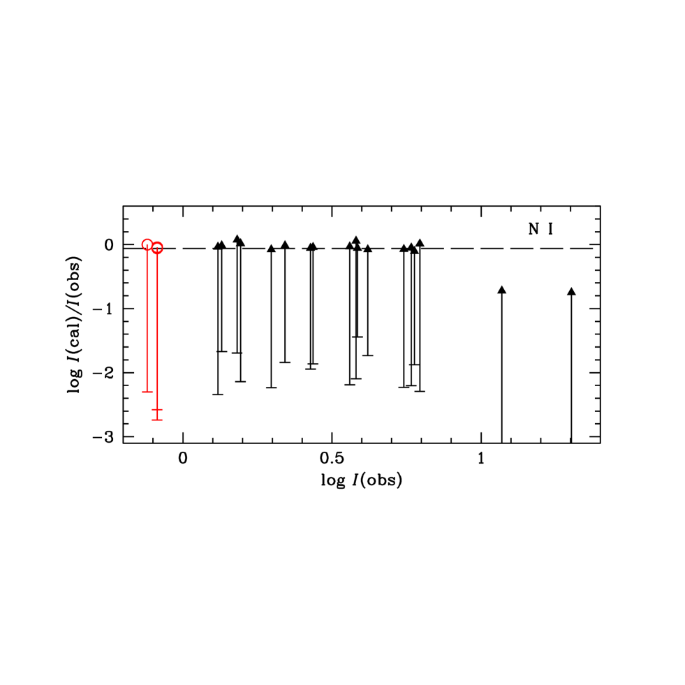
Figure 5: Same as in Fig. 2 for N i lines. Collisionally excited forbidden lines are also included.

where $R$ is the distance to the central star in cm. Table 4 gives the adopted values for parameters $n_{0\ldots 2}$, $R_{\rm in}$, $R_{1}$, $R_{2}$, $\sigma_{1}$ and $\sigma_{2}$. Parameters $R_{1}$, $R_{2}$ have intermediate values between the long and short axes in the ellipsoidal model of MG. This density profile was chosen to match the HST images of the intense nebular lines as discussed in detail by MG (see their figure 5). With few exceptions, the predicted line intensities in our 1D model vary by less than 30 per cent when $n_{0\ldots 2}$ are varied simultaneously by 20 per cent or when $R_{1}$ and $R_{2}$ are varied simultaneously by 20 per cent.

Table 3: Element abundances in the nebular model

Element	$\log{\rm X/H}$
He	$-0.92$
C	$-3.10$
N	$-4.00$
O	$-3.40$
Ne	$-4.00$
Mg	$-4.95$
Si	$-4.90$
S	$-5.35$
Cl	$-6.90$
Ar	$-5.80$
Fe	$-7.40$

Table 4: Nebular density profile parameters

Parameter	Unit	Value
$\lx@intercol n_{0}\hfil$	$\,\rm cm^{-3}$	2850
$\lx@intercol n_{1}\hfil$	$\,\rm cm^{-3}$	5260
$\lx@intercol n_{2}\hfil$	$\,\rm cm^{-3}$	9500
$\lx@intercol n_{3}\hfil$	$\,\rm cm^{-3}$	20500
$\lx@intercol\log R_{\rm in}\hfil$	cm	16.06
$\lx@intercol\log R_{1}\hfil$	cm	16.28
$\lx@intercol\log R_{2}\hfil$	cm	17.02
$\lx@intercol\log R_{3}\hfil$	cm	17.10
$\lx@intercol\log\sigma_{1}\hfil$	cm	15.96
$\lx@intercol\log\sigma_{2}\hfil$	cm	16.46

4.3 The photodissociation region

It has long been known that IC 418 has a PhotoDissociation Region (PDR) extending beyond the optical nebula (Cohen & Barlow, 1974; Taylor & Pottasch, 1987) with low ionization and atomic components (Monk, Barlow & Clegg, Monk et al.1990, Taylor et al.1989; Meixner et al., 1996). (Taylor et al.1989) measured an H mass of $0.35\pm 0.05\,$M☉ over a radius $\ga 90\,$arcsec from the center of the nebula. Thus far there have been no detections of molecular emission in IC 418 (Huggins et al., 1996; Dayal & Bieging, 1996; , Hora et al.1999). Liu et al. (2001a) obtained an average density for the PDR of $10^{5.5}\mbox{$\,\rm cm^{-3}$}$ from observations of the [C ii] 158–$\,\mu$m and [O i] 63–$\,\mu$m and 146–$\,\mu$m lines. That density is much higher than the one needed to explain the radio observations and suggests the existence of a narrow dense shell just outside the ionization front or clumps in the PDR.

The cloudy nebular model can be readily extended to the PDR by adding an outer neutral atomic envelope to the ionized region starting at a distance of the central star $R_{3}$. We chose the following density profile for the PDR:

$$n_{\rm PDR}(R>R_{3})=n_{3}(T_{e}/10^{4}\mbox{$\,\rm K$})^{-1.2}$$ (7)

where $T_{e}$ is the electron temperature in kelvins, and $n_{3}$ and $R_{3}$ are given in table 4. This density profile is constrained by the observed fluxes of the FIR [C ii] and [O i] lines. The temperature dependence in Eq. (7) allows for a smooth transition between the ionized and neutral material by increasing the density as the temperature drops. The extent of the neutral region needed to match the observed intensities of the FIR O i and C ii lines is just a few percent of the radius of the ionized region. A more realistic model of the ionized and molecular interface needs a hydrodynamic model, which is beyond the scope of this paper.

5 Results

5.1 Selection of observations

Proper line identification of weak spectral lines is a fundamental problem in the analysis of deep nebular spectroscopy. SWBH presented the line identification code emili to automate and standarise an otherwise tedious labour of identifying several hundreds of spectral lines. SBW selected a subset of emission line intensities from the survey of SWBH based on the likelihood of a correct, unique identification as given by emili and the availability of published effective recombination coefficients to determine abundances. Some lines in SWBH were not taken into account by SBW because those lines were probably blended with other emission lines or emili gave more than one plausible identification for them.

We have reexamined the SWBH line list and added many measured lines of C ii, N i, N ii, O i and O ii to the selection of SBW in order to compare them with our calculations either because we could estimate their effective recombination coefficients reasonably well or because they were the most probable contributor to a blend. Some cases for individual species are discussed in the following sections.

Published calculations often tabulate the line effective recombination coefficient in equation (3) for the most intense lines only. Coefficients for weaker lines with the same upper state $j$ can be readily estimated by dividing by the branching ratio $P_{ji}$ of the tabulated transition and multiplying by the corresponding $P_{ji}$ of the desired line as in equation (2). In order to do this consistently, it is necessary that authors publish the transition probability data or at least the branching ratios used in their calculations (Nussbaumer & Storey, 1984; Escalante & Victor, 1990; , Pequignot et al.1991; Escalante & Victor, 1992; Liu et al., 1995).

The issue of multiple identifications is more complicated. A line with multiple identifications may be either a real blend or some of the proposed identifications may not be real. Our calculations show that in many cases a transition in a possible blend contributes insignificantly to the measured intensity. When a transition in a blend of two transitions of the same species contributes more than 10 per cent of the total intensity, we have added the calculated intensities of the transitions to compare them with the measurements by SWBH. Blends of emissions of the same species are thus compared with our computed spectra without the need to assume theoretical intensities to ‘deblend’ the observed lines. Blends of emissions of different species are compared directly with the predicted intensities.

5.2 Comparison with observed intensities

In Fig. 2 to 6 we compare predicted intensities with observed intensities in a scale of $I(\mbox{$\rm H\beta$})=10^{4}$. Tables 5 to 14 give the predicted intensities of dipole–allowed lines with intensities higher than $8\times 10^{-6}$ of the $\rm H\beta$ strength, which is close to the lower limit of detection in SWBH. Tables 13 and 14 also include predicted intensities of the optical forbidden lines of N i and O i. Some of the wavelengths given in the second column of the table are calculated from energy levels and have limited accuracy. The fraction of calculated intensity due to recombination is given in the third column of the tables. The calculated and observed intensities in the fourth and fifth columns are normalized to $I(\mbox{$\rm H\beta$})=10^{4}$. The bottom line in each table gives the average of the ratio of the intensity due to recombination to the total calculated intensity and the average of the ratio of the calculated intensity to the observed intensity for each species. We have found some undetected lines with calculated intensities above the detection limit in SWBH. Some of them are blended with intense nebular lines, and a few were measured, but apparently not identified by emili. The observed intensity of lines not selected by SBW are marked with ‘?’ in the sixth column of the tables.

The uncertainty of each line intensity depends on several factors like the signal–to–noise ratio ($\rm S/N$), its relative width with respect to the instrument resolution and whether the line may be blended with other lines. In order to make meaningful comparisons with observations, MG estimated a variable uncertainty of the line fluxes in SBW between 10 per cent for the brighter lines to 30 per cent for the weaker lines. SBW suggest an uncertainty of 20 per cent for lines with a $\rm S/N>20$. Most of the lines analysed in this work are weaker than 0.01 times the intensity of $\rm H\beta$, and have a $\rm S/N>20$. Therefore we will adopt a minimum general uncertainty of 20 per cent for all dipole–allowed lines in the SWBH survey.

Our calculations tend to underestimate most of the lines with dubious identification according to emili. Rola & Pela (1994) and Wesson, Stock & Scicluna (Wesson et al.2012) have shown that measured intensities of lines with $\rm S/N<6$ are strongly biased upwardly. We only have two lines with an underestimated predicted intensity and a measured $\rm S/N<7$, which corresponds to a true $\rm S/N$ between 6 and 8 at the 1–$\sigma$ confidence level according to the calculations of Rola & Pela (1994). In most of our cases it is more likely that the underestimated predictions indicate incorrect identifications or blends with other lines rather than uncertainties in the measured values. We have not included in the tables and figures features with a dubious identification and a predicted intensity less than 0.1 of the measured value.

The excitation mechanisms of a spectrum can be diagnosed by contrasting the intensities of lines yielded by different atomic configurations as done by Grandi (1975, 1976). Lines from s, p and most d states with the same spin multiplicity as that of the ground state are enhanced in varying degrees by fluorescence relative to recombination lines if the recombined ion concentration is sufficiently high. Transitions from d states that are not connected to the ground or a metastable state by a resonant transition and transitions from f and g states are excited mostly or totally by recombination.

SBW found that some dipole–allowed lines of a species have profiles similar to those of the forbidden lines of the next higher ionization stage of the species, (e.g. some O i line profiles are similar to [O ii] profiles), indicating that they are produced in the same part of the nebula by recombination of the more ionized stage. Likewise they found that other dipole–allowed lines of the same species have profiles similar to those of the forbidden lines of the same ionization stage, indicating that they are produced by fluorescence excitation of that species.

SBW also found a correlation between the line width of the species producing the line and the ionization potential of the species, which indicates a relationship between the line width and the ionization stratification in the nebula. Recombination lines of species with lower ionization potential generally have broader lines and their widths are similar to those of the forbidden lines of the next higher ionization stage, indicating again a common place of origin within the nebula.

SBW proposed that line profile and line width similarities can be used to discriminate the excitation mechanism of the lines. The contributions of fluorescence and recombination, however, are comparable in many lines and produce many exceptions to the discriminating criteria proposed by SBW as discussed for particular cases below. Therefore a more quantitative analysis is needed to determine the excitation mechanism of a line.

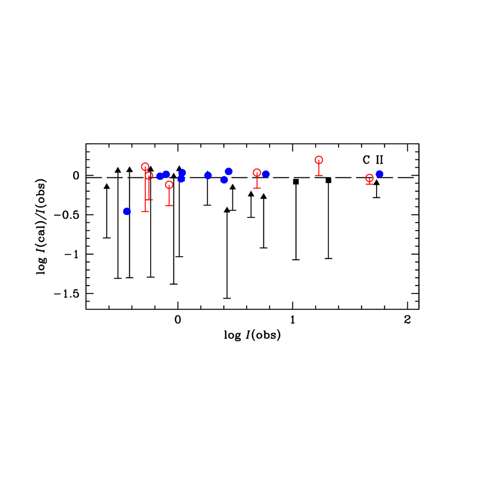
Figure 2: Comparison of C ii intensities observed by SBW with predicted intensities produced by recombination and fluorescence of lines from s states (black squares), p states (black triangles), d states (open red circles), and f and g states (filled blue circles). The dash at the bottom of the vertical lines marks the intensity produced by recombination excitation only. The broken horizontal line is the average value of $I_{\rm cal}/I_{\rm obs}$. Note that the observed intensities are normalized to $I(\mbox{$\rm H\beta$})=10^{4}$.

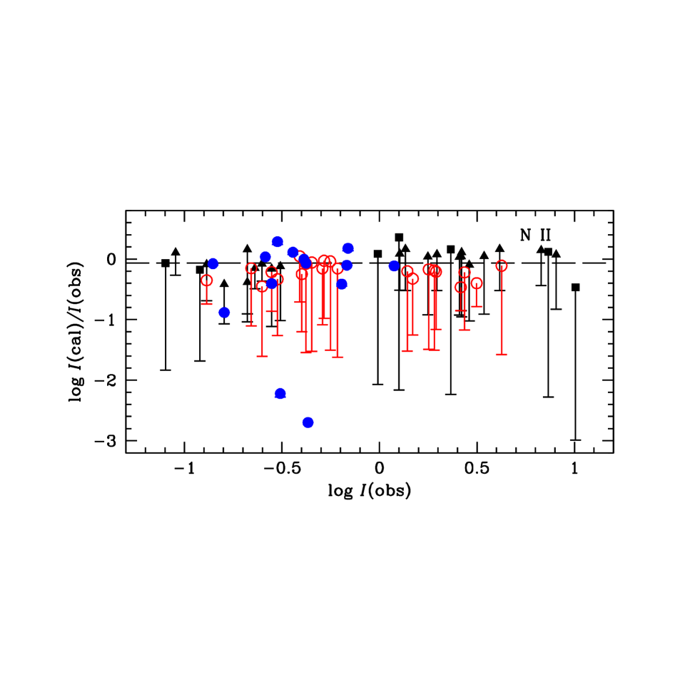
Figure 3: Same as in Fig. 2 for N ii lines.

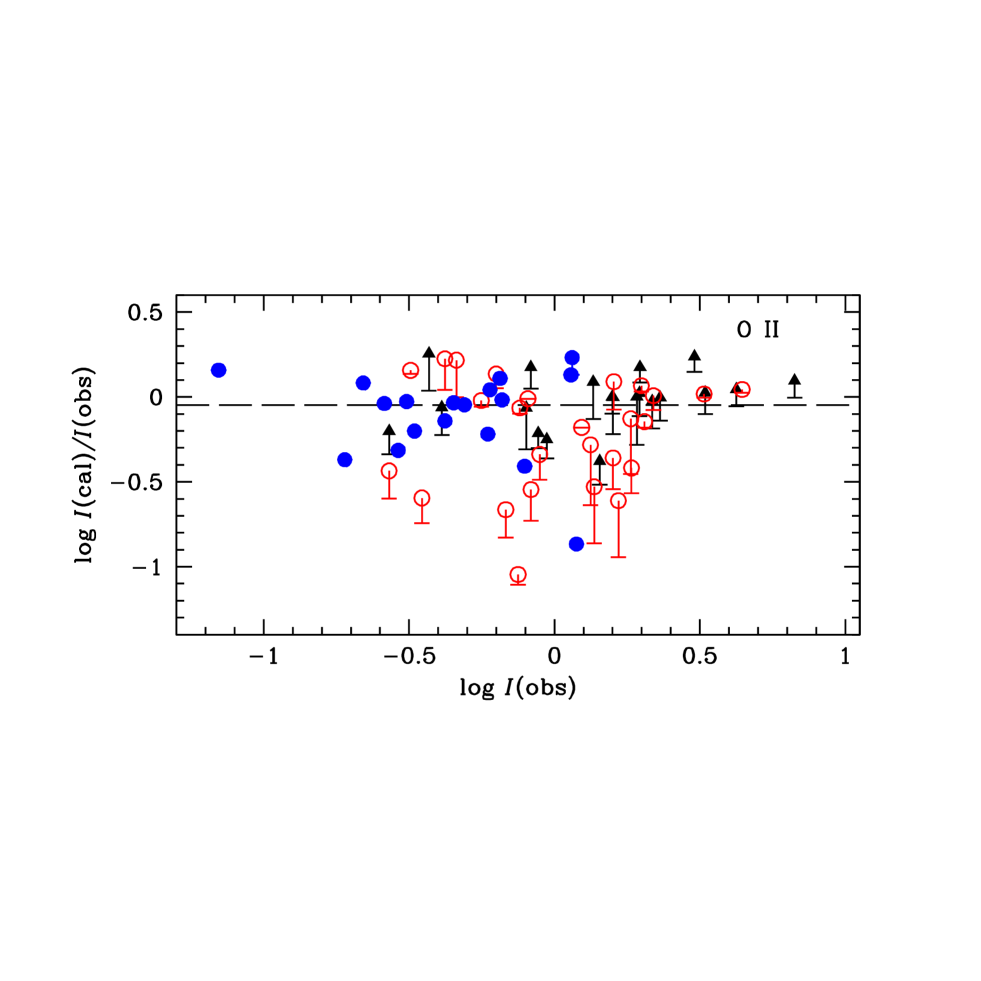
Figure 4: Same as in Fig. 2 for O ii lines.

5.3 C ii

The agreement of predicted recombination intensities within 20 per cent of observed values in the SBW selection of 9 lines or blends of lines from f and g states supports the accuracy of the recombination rates for this ion. That remarkable consistency can be explained by three factors concerning the observed high angular momentum states: those states are less dependent on atomic calculation assumptions because of their reduced non–hydrogenic effects, their populations are free from optical depth effects, and their fine–structure components are often blended in spectroscopic terms. In those blends, the effective transition rate of the term is a weighted average of several fine structure transition probabilities so that the total intensity of the blend is the sum of intensities of those components. Quantum calculations with different assumptions tend to agree on the transition probabilities for the more intense components of a term. The average tends to cancel out differences in the calculated $A$–values of the fine structure components while the summation gives more weight to the components with the larger intensities and lower observational errors. Measurement errors are also expected to decrease with the higher S/N of a blend of several lines belonging to the same term.

Recombinations produce more than half the intensity of most C ii lines, but we find an important fluorescence contribution to all the observed lines from s, p and d states. SBW did not find differences in the line profiles of those lines with profiles of recombination lines as should be indicated by their proposed criteria based on line profile differentiation. The fluorescence contribution is particularly important in multiplets $\rm 3p\ ^{2}P^{o}$–$\rm 4s\ ^{2}S_{1/2}$$\lambda\lambda\,$3918.97, 3920.68, $\rm 4p\ ^{2}P^{o}$–$\rm 6d\ ^{2}D$$\lambda\lambda\,$4637.63–4639.07, $\rm 3d\ ^{2}D$–$\rm 4p\ ^{2}P^{o}$$\lambda\lambda\,$5889.28–5891.60, $\rm 4p\ ^{2}P^{o}$–$\rm 5d\ ^{2}D$$\lambda\lambda\,$6257.18–6259.80, and $\rm 3s\ ^{2}S_{1/2}$–$\rm 3p\ ^{2}P^{o}$$\lambda\lambda\,$6578.05, 6582.88, and it is mostly due to absorptions from the ground state in the doublet $\rm 2p\ ^{2}P^{o}$–$\rm 4s\ ^{2}S$$\lambda\lambda\,$636.994, 636.251, and the triplets $\rm 2p\ ^{2}P^{o}$–$\rm 5d\ ^{2}D$$\lambda\lambda\,$560.239–560.439, $\rm 2p\ ^{2}P^{o}$–$\rm 6d\ ^{2}D$$\lambda\lambda\,$543.258–543.445, followed by decays to term $\rm 4p\ ^{2}P^{o}$. This fluorescence excitation explains the enhanced intensities of those multiplets relative to the recombination lines, and the seemingly high $\rm C^{2+}$ abundances derived from their intensities by SBW using recombination rates alone.

We added 13 lines from the SWBH survey with excited–core upper terms $\rm 2s2p(^{3}P^{o})3p\ ^{2}P$ and $\rm 2s2p(^{3}P^{o})3p\ ^{2}D$ and two lines from the $\rm 9f\ ^{2}F^{o}$ term using additional effective recombination coefficients of (Davey et al.2000) published on line at the CDS site. Term $\rm 2s2p(^{3}P^{o})3p\ ^{2}P$ is mostly excited by fluorescence through absorptions in multiplet $\rm 2p\ ^{2}P^{o}$–$\rm 2s2p(^{3}P^{o})3p\ ^{2}P$$\lambda\lambda\,$549.320–549.570. The calculated intensities for decays from that term agree with the observations within our adopted uncertainty intervals except for the line $\rm 2p^{3}\ {}^{2}P^{o}_{1/2}$–$\rm 2s2p(^{3}P^{o})3p\ ^{2}P_{3/2}$$\lambda\,$7508.89 apparently undetected by SWBH, and the line $\rm 4p\ ^{2}P_{3/2}$–$\rm 2s2p(^{3}P^{o})3p\ ^{2}P_{3/2}$$\lambda\,$5121.83 underestimated by a factor of 2.8. Lines from term $\rm 2s2p(^{3}P^{o})3p\ ^{2}D$ on the other hand are underestimated by our calculations by 30 to 50 per cent. Lines from the state $\rm 2s2p(^{3}P^{o})3p\ ^{2}D_{3/2}$ have a 70 per cent excitation by fluorescence while lines from the other state $\rm 2s2p(^{3}P^{o})3p\ ^{2}D_{5/2}$ have a 40 per cent excitation by fluorescence mainly in absorptions in multiplet $\rm 2p\ ^{2}P^{o}$–$\rm 2s2p(^{3}P^{o})3p\ ^{2}D$$\lambda\lambda\,$530.275–530.474. The relatively intense line $\rm 4p\ ^{2}P^{o}_{1/2}$–$\rm 2s2p(^{3}P^{o})3p\ ^{2}D_{3/2}$$\lambda\,$3835.72 is probably blended with the Balmer H9 line. The two blended lines $\rm 5d\ ^{2}D_{5/2}$–$\rm 9f\ ^{2}F^{o}_{5/2}$ and $\rm 5d\ ^{2}D_{5/2}$–$\rm 9f\ ^{2}F^{o}_{7/2}$ at $\lambda\,$7860.50 are the only f multiplet with a strong discrepancy with observations with an observed intensity 2.8 times larger than the predicted intensity. The discrepancy may be due to uncertainties in the measurement because the observed S/N of 28.7 in SWBH is lower than the other C ii blends of f and g states and the intensity of the other blend from the $\rm 9f\ ^{2}F$ term is within the uncertainty interval of the observed value.

Table 5: Predicted and observed line intensities of C ii. $I_{\rm rec}/I_{\rm calc}$ is the fraction of the calculated intensity due to recombination, $I_{\rm calc}$ is the predicted intensity, $I_{\rm obs}$ is the measured intensity with a 20 per cent minimum uncertainty. The ? marks measured intensities taken from SWBH, but not selected by SBW.

Lower–Upper	$\lambda\,$(Å)	$I_{\rm rec}/I_{\rm calc}$	$I_{\rm calc}$	$I_{\rm obs}$
$\rm 4p\ ^{2}P^{o}_{3/2}$–$\rm 3p^{\prime}\ {}^{2}D_{5/2}$$\dagger$	3831.7	0.512	2.10	3.00 ?
$\rm 4p\ ^{2}P^{o}_{1/2}$–$\rm 3p^{\prime}\ {}^{2}D_{3/2}$	3835.7	0.226	2.51	—
$\rm 4p\ ^{2}P^{o}_{3/2}$–$\rm 3p^{\prime}\ {}^{2}D_{3/2}$	3836.7	0.226	0.50	—
$\rm 3p\ ^{2}P^{o}_{1/2}$–$\rm 4s\ ^{2}S_{1/2}$	3919.0	0.102	8.87	10.68
$\rm 3p\ ^{2}P^{o}_{3/2}$–$\rm 4s\ ^{2}S_{1/2}$	3920.7	0.102	17.70	20.52
$\rm 3d\ ^{2}D_{5/2}$–$\rm 4f\ ^{2}F^{o}_{7/2}$	4267.3	0.989	59.20	57.12
$\rm 4f\ ^{2}F^{o}$–$\rm 10g\ ^{2}G$ §	4292.2	1.000	0.81	0.79
$\rm 4d\ ^{2}D$–$\rm 9f\ ^{2}F^{o}$	4329.7	0.954	0.68	0.70
$\rm 4f\ ^{2}F^{o}$–$\rm 9g\ ^{2}G$	4491.1	1.000	1.18	1.09
$\rm 4d\ ^{2}D$–$\rm 8f\ ^{2}F^{o}$	4618.8	0.942	0.97	1.07
$\rm 4p\ ^{2}P^{o}_{1/2}$–$\rm 6d\ ^{2}D_{3/2}$	4637.6	0.492	0.56	0.56
$\rm 4p\ ^{2}P^{o}_{3/2}$–$\rm 6d\ ^{2}D_{5/2}$	4638.9	0.807	0.65	—
$\rm 4p\ ^{2}P^{o}_{3/2}$–$\rm 6d\ ^{2}D_{3/2}$	4639.1	0.492	0.11	—
$\rm 2p^{2}\ {}^{2}P_{3/2}$–$\rm 3p\ ^{2}P^{o}_{3/2}$	4744.8	0.654	0.09	—
$\rm 4f\ ^{2}F^{o}$–$\rm 8g\ ^{2}G$	4801.9	1.000	1.82	1.83
$\rm 2p^{3}\ {}^{2}P^{o}_{3/2}$–$\rm 3p^{\prime}\ {}^{2}D_{5/2}$	5032.1	0.512	2.48	4.34 ?
$\rm 2p^{3}\ {}^{2}P^{o}_{1/2}$–$\rm 3p^{\prime}\ {}^{2}D_{3/2}$	5035.9	0.226	2.97	5.58 ?
$\rm 2p^{3}\ {}^{2}P^{o}_{3/2}$–$\rm 3p^{\prime}\ {}^{2}D_{3/2}$	5040.7	0.226	0.59	—
$\rm 4p\ ^{2}P^{o}_{1/2}$–$\rm 3p^{\prime}\ {}^{2}P_{3/2}$	5120.1	0.077	0.19	—
$\rm 4p\ ^{2}P^{o}_{3/2}$–$\rm 3p^{\prime}\ {}^{2}P_{3/2}$	5121.8	0.077	0.96	2.68 ?
$\rm 4p\ ^{2}P^{o}_{1/2}$–$\rm 3p^{\prime}\ {}^{2}P_{1/2}$	5125.2	0.043	0.69	0.58 ?
$\rm 4p\ ^{2}P^{o}_{3/2}$–$\rm 3p^{\prime}\ {}^{2}P_{1/2}$	5127.0	0.043	0.34	0.30 ?
$\rm 4f\ ^{2}F^{o}$–$\rm 7g\ ^{2}G$	5341.5	1.000	3.11	2.77
$\rm 3d\ ^{2}D_{3/2}$–$\rm 4p\ ^{2}P^{o}_{3/2}$	5889.3	0.506	0.30	—
$\rm 3d\ ^{2}D_{5/2}$–$\rm 4p\ ^{2}P^{o}_{3/2}$	5889.8	0.506	2.69	—
$\rm 3d\ ^{2}D_{3/2}$–$\rm 4p\ ^{2}P^{o}_{1/2}$	5891.6	0.406	1.86	1.81
$\rm 4d\ ^{2}D$–$\rm 6f\ ^{2}F^{o}$	6145.9	0.969	2.22	2.53
$\rm 4p\ ^{2}P^{o}_{1/2}$–$\rm 5d\ ^{2}D_{3/2}$	6257.2	0.270	0.67	0.52
$\rm 4p\ ^{2}P^{o}_{3/2}$–$\rm 5d\ ^{2}D_{5/2}$	6259.6	0.544	0.64	0.84
$\rm 4p\ ^{2}P^{o}_{3/2}$–$\rm 5d\ ^{2}D_{3/2}$	6259.8	0.270	0.13	—
$\rm 4f\ ^{2}F^{o}$–$\rm 6g\ ^{2}G$	6460.1	1.000	6.04	5.84
$\rm 3s\ ^{2}S_{1/2}$–$\rm 3p\ ^{2}P^{o}_{3/2}$	6578.1	0.654	42.90	53.74
$\rm 3s\ ^{2}S_{1/2}$–$\rm 3p\ ^{2}P^{o}_{1/2}$	6582.9	0.527	26.60	—
$\rm 3p\ ^{2}P^{o}_{1/2}$–$\rm 3d\ ^{2}D_{3/2}$	7231.3	0.632	26.60	16.92
$\rm 3p\ ^{2}P^{o}_{3/2}$–$\rm 3d\ ^{2}D_{5/2}$	7236.4	0.836	43.30	46.73
$\rm 3p\ ^{2}P^{o}_{3/2}$–$\rm 3d\ ^{2}D_{3/2}$	7237.2	0.632	5.30	4.89
$\rm 5f\ ^{2}F^{o}_{5/2}$–$\rm 10g\ ^{2}G_{7/2}$	7508.9	1.000	0.17	—
$\rm 5f\ ^{2}F^{o}_{7/2}$–$\rm 10g\ ^{2}G_{9/2}$	7508.9	1.000	0.23	—
$\rm 2p^{3}\ {}^{2}P^{o}_{1/2}$–$\rm 3p^{\prime}\ {}^{2}P_{3/2}$	7508.9	0.077	0.25	—
$\rm 2p^{3}\ {}^{2}P^{o}_{3/2}$–$\rm 3p^{\prime}\ {}^{2}P_{3/2}$	7519.5	0.077	1.23	1.03 ?
$\rm 2p^{3}\ {}^{2}P^{o}_{1/2}$–$\rm 3p^{\prime}\ {}^{2}P_{1/2}$	7519.9	0.043	0.89	0.92 ?
$\rm 2p^{3}\ {}^{2}P^{o}_{3/2}$–$\rm 3p^{\prime}\ {}^{2}P_{1/2}$	7530.6	0.043	0.44	0.38 ?
$\rm 5d\ ^{2}D_{3/2}$–$\rm 9f\ ^{2}F^{o}_{5/2}$	7860.2	0.943	0.09	—
$\rm 5d\ ^{2}D_{5/2}$–$\rm 9f\ ^{2}F^{o}_{5/2}$	7860.5*	0.962	0.13	0.36 ?
$\rm 5f\ ^{2}F^{o}_{5/2}$–$\rm 9g\ ^{2}G_{7/2}$	8139.6	1.000	0.24	—
$\rm 5f\ ^{2}F^{o}_{7/2}$–$\rm 9g\ ^{2}G_{9/2}$	8139.6	1.000	0.31	—
$\rm 5d\ ^{2}D_{3/2}$–$\rm 8f\ ^{2}F^{o}_{5/2}$	8867.6	0.923	0.11	—
$\rm 5d\ ^{2}D_{5/2}$–$\rm 8f\ ^{2}F^{o}_{7/2}$	8868.1	0.956	0.16	—

§ Terms with no subscript are blended transitions of several states of angular momentum $J$.
$\dagger$ 3p’ is core excited configuration $\rm 2s2p(^{1}D^{o})3p$.
*$\lambda\,$7860.5 includes blend with $\rm 5d\ ^{2}D_{5/2}$–$\rm 9f\ ^{2}F^{o}_{7/2}$.

Table 6: continued

Lower–Upper	$\lambda\,$(Å)	$I_{\rm rec}/I_{\rm calc}$	$I_{\rm calc}$	$I_{\rm obs}$
$\rm 5f\ ^{2}F^{o}_{7/2}$–$\rm 8g\ ^{2}G_{9/2}$	9221.1	1.000	0.45	—
$\rm 5f\ ^{2}F^{o}_{5/2}$–$\rm 8g\ ^{2}G_{7/2}$	9221.1	1.000	0.35	—
$\rm 3s^{\prime}\ {}^{2}P^{o}_{3/2}$–$\rm 3p^{\prime}\ {}^{2}D_{5/2}$	9238.3	0.512	0.14	—
$\rm 3s^{\prime}\ {}^{2}P^{o}_{1/2}$–$\rm 3p^{\prime}\ {}^{2}D_{3/2}$	9251.0	0.226	0.17	0.24 ?
$\langle I_{\rm rec}/I_{\rm calc}\rangle=0.581$		$\langle I_{\rm calc}/I_{\rm obs}\rangle=0.938$

5.4 N ii

Fluorescence is the main excitation mechanism for most N ii lines in IC 418, but to a lesser extent than in the Orion nebula. The main pumping mechanisms in this ion were discussed in detail by Escalante and Morisset (2005). The $\rm{}^{3}P$ ground core offers several pumping channels to the $\rm 3d\ ^{3}P^{o}$ and $\rm 3d\ ^{3}D^{o}$ terms through multiplets $\rm 2p^{2}\ {}^{3}P$–$\rm 3d\ ^{3}P^{o}$$\lambda\lambda\,$529.36–529.87, $\rm 2p^{2}\ {}^{3}P$–$\rm 3d\ ^{3}D^{o}$$\lambda\lambda\,$533.51–533.88 and $\rm 2p^{2}\ {}^{3}P$–$\rm 4s\ ^{3}P^{o}$$\lambda\lambda\,$508.48–509.01. The only 3d term with significant recombination excitation is $\rm 3d\ ^{3}F^{o}$, but its brightest components at $\lambda\lambda\,$5001.13, 5001.13 and 5005.15 are blended with the [O iii]$\lambda\,$5006.84 nebular line. The singlet lines $\rm 3p\ ^{1}P_{1}$–$\rm 3d\ ^{1}D^{o}_{2}$$\lambda\,$4447.03 and $\rm 3p\ ^{1}D_{2}$–$\rm 3d\ ^{1}F^{o}_{3}$$\lambda\,$6610.56 listed by SBW are also excited mostly by fluorescence due to absorptions in the transitions $\rm 2p\ ^{3}P_{1}$–$\rm 3d\ ^{1}D^{o}_{2}$$\lambda\,$534.657 and $\rm 2p\ ^{1}D_{2}$–$\rm 3d\ ^{1}F^{o}_{3}$$\lambda\,$574.650 respectively. The first one is a spin–forbidden transition with the ground triplet term while the second demonstrates that a metastable state can also produce fluorescence excitation.

The disagreement of observed intensities with predicted intensities in lines excited by fluorescence is greater in this ion. There is a systematic underestimation of the calculated values of lines from 3d states of 30 to 70 per cent. The rest of the calculated intensities selected by SBW are within 40 per cent of the observed values.

The 4f states are populated by recombination. Direct recombinations and transitions from the 4f states produce between 30 and 60 per cent of the intensity of the lines from the $\rm 3d\ ^{3}D^{o}$ and $\rm 3d\ ^{3}F^{o}$ terms. EM showed that fluorescence cannot significantly populate f and higher angular momentum states in $\rm N^{+}$ because quantum probabilities strongly favour downward transitions with decreasing angular momentum. That is a well known trend of transition probabilities inferred from atomic data compilations and theoretical considerations (Khriplovich & Matvienko, 2007). Consequently d states have a greater probability of decaying to p states than to f states. Should fluorescence enhance an f state population by decays from a higher d state, lines from lower p states, like $\rm 3s\ ^{3}P^{o}_{2}$–$\rm 3p\ ^{3}P_{2}$$\lambda\,$4630.54, would show at least a 70 per cent enhancement in their predicted intensity (EM). In our present calculations that line is already overpredicted by 20 per cent above its observed value without any plausible fluorescence contribution to f states. The enhanced intensity of the $\rm 3s\ ^{3}P^{o}_{2}$–$\rm 3p\ ^{3}D_{3}$$\lambda\,$5679.56 line by fluorescence in IC 418 puts its ratio with the recombination line $\rm 3d\ ^{3}F^{o}_{4}$–$\rm 4f\ G[9/2]_{5}$$\lambda\,$4041.31 out of the $T_{e}$ and $n_{e}$ ranges in fig. 8 of FSL, and highlights the importance of determining the atomic processes that excite a line before it is used as a diagnostic tool.

We have added 15 lines from the SWBH survey that were omitted in the analysis of SBW. Some like $\rm 3d\ ^{3}D^{o}_{2}$–$\rm 4f\ F[5/2]_{3}$$\lambda\,$4241.76, and $\rm 3d\ ^{3}D^{o}_{3}$–$\rm 4f\ F[7/2]_{4}$$\lambda\,$4241.78 are blended, and $\rm 3d\ ^{3}D^{o}_{2}$–$\rm 4f\ F[7/2]_{3}$$\lambda\,$4237.05 is probably blended with the transition $\rm 3d\ ^{3}D^{o}_{1}$–$\rm 4f\ F[5/2]_{2}$$\lambda\,$4236.91 listed in the selection of SBW. There are four lines standing out from f states with predicted intensities significantly below the observed values: $\rm 3d\ ^{3}F^{o}_{4}$–$\rm 4f\ G[7/2]_{3}$$\lambda\,$4058.16, $\rm 3d\ ^{1}D^{o}_{2}$–$\rm 4f\ F[5/2]_{3}$$\lambda\,$4176.16, $\rm 3d\ ^{3}D^{o}_{3}$–$\rm 4f\ F[5/2]_{2}$$\lambda\,$4246.71, $\rm 3d\ ^{3}P^{o}_{0}$–$\rm 4f\ D[3/2]_{1}$$\lambda\,$4433.48, and $\rm 4d\ ^{1}F_{3}$–$\rm 5f\ G[9/2]_{4}$$\lambda\,$9794.05, which are discussed below.

Because there is only one more line from a 4f D term with a secure identification ($\rm 3d\ ^{1}P^{o}_{1}$–$\rm 4f\ D[3/2]_{2}$$\lambda\,$4678.14) and an intensity 15 per cent above the predicted value, we cannot assert whether the effective recombination coefficient of the $\lambda\,$4433.48 line is underestimated. The other line produced by a 4f D term listed in SWBH, $\rm 3d\ ^{3}P^{o}_{2}$–$\rm 4f\ D[5/2]_{3}$$\lambda\,$4432.74, may be blended with a [Fe II] line, but our calculations predict an intensity 30 per cent above the measured value. The effective recombination coefficients of FSL and EV at $10^{4}\mbox{$\,\rm K$}$ agree for the lines of multiplet $\rm 3d\ ^{3}P^{o}$–$\rm 4f\ D[5/2]$$\lambda\lambda\,$4432.74–4442.02.

Our calculations predict intensities 0.002 times and 0.006 times the observed intensities of the lines $\lambda\,$4058.16 and $\lambda\,$4246.71 respectively. The low S/N of 10.3 and 9.2 and the displacement between the tabulated and observed wavelength of $10.3\mbox{$\,\rm km\,s^{-1}$}$ and $9.2\mbox{$\,\rm km\,s^{-1}$}$ respectively reported by SWBH for those lines suggest that they may be misidentifications. Other lines of the term $\rm 4f\ F[5/2]$, like $\rm 3d\ ^{1}D^{o}_{2}$–$\rm 4f\ F[5/2]_{3}$$\lambda\,$4176.16, with more secure identifications also show important differences with the calculated values.

The dispersion of calculated intensities above and below the observed values of transitions from 4f D and 4f F terms may imply uncertainties in the recombination coefficients or uncertainties in the measurements due to the low signal to noise ratio. There are no significant differences between the effective recombination coefficients of FSL and EV for those lines as shown in table 1.

For the lines from 4f G terms the agreement between predicted and observed intensities is within 20 per cent for nearly all lines. The only exception is the line $\rm 3d\ ^{3}F^{o}_{4}$–$\rm 4f\ G[7/2]_{3}$ $\lambda\,$4058.16 mentioned above with an effective recombination coefficient by FSL more than twice the value of EV. Even so, the value by FSL is not large enough to explain its intensity if it is indeed N ii emission.

Finally the line $\rm 4d\ ^{1}F_{3}$–$\rm 5f\ G[9/2]_{4}$$\lambda\,$9794.05 is the only line from a $\rm 5f\ G$ term above the detection limit, and is strongly underestimated by a factor of 7.6 in intensity, with a S/N of 9.0 and no alternative identifications.

The line at $\lambda\,$4674.903 was measured but not identified by SWBH. Our calculations predict the N ii spin–forbidden transition $\rm 3s\ ^{1}P^{o}_{1}$–$\rm 3p\ ^{3}P_{0}$$\lambda\,$4674.91 to be a most likely identification. The transition probability given by Froese Fischer & Tachiev (2004) of $8.54\times 10^{6}\mbox{$\,\rm s^{-1}$}$ overestimates the observed value by 40 per cent. The other two members of this N ii multiplet, $\rm 3s\ ^{1}P^{o}_{1}$–$\rm 3p\ ^{3}P_{2}$$\lambda\,$4654.53 and $\rm 3s\ ^{1}P^{o}_{1}$–$\rm 3p\ ^{3}P_{1}$$\lambda\,$4667.21, were identified by SWBH as the O i multiplet $\rm 3p\ ^{5}P$–$\rm 8d\ ^{5}D^{o}$$\lambda\,$4654.56 and the line [Fe iii] $\rm 3d^{6}\ {}^{5}D_{3}$–$\rm 3d^{6}\ {}^{3}F2_{2}$$\lambda\,$4667.010 respectively. Our calculations predict an intensity 0.09 times weaker than the observed value for the O i multiplet (see section 5.8) while the agreement with predicted intensities for both lines is much better if our proposed identifications as N ii lines are correct.

Table 7: Predicted and observed line intensities of N ii.

Lower–Upper	$\lambda\,$(Å)	$I_{\rm rec}/I_{\rm calc}$	$I_{\rm calc}$	$I_{\rm obs}$
$\rm 3p\ ^{3}S_{1}$–$\rm 4s\ ^{3}P^{o}_{2}$	3593.6	0.004	1.79	—
$\rm 3p\ ^{3}S_{1}$–$\rm 4s\ ^{3}P^{o}_{1}$	3609.1	0.003	1.41	—
$\rm 3p\ ^{3}S_{1}$–$\rm 4s\ ^{3}P^{o}_{0}$	3615.9	0.007	0.22	—
$\rm 3p\ ^{3}P_{1}$–$\rm 4s\ ^{3}P^{o}_{2}$	3829.8	0.004	3.36	2.32
$\rm 3p\ ^{3}P_{2}$–$\rm 4s\ ^{3}P^{o}_{2}$	3838.4	0.004	9.68	7.34 ?
$\rm 3p\ ^{3}P_{0}$–$\rm 4s\ ^{3}P^{o}_{1}$	3842.2	0.003	2.87	1.26
$\rm 3p\ ^{3}P_{1}$–$\rm 4s\ ^{3}P^{o}_{1}$	3847.4	0.003	2.08	—
$\rm 3p\ ^{3}P_{1}$–$\rm 4s\ ^{3}P^{o}_{0}$	3855.1	0.007	1.19	0.98
$\rm 3p\ ^{3}P_{2}$–$\rm 4s\ ^{3}P^{o}_{1}$	3856.1	0.003	3.47	10.13 ?
$\rm 3d\ ^{3}F^{o}_{3}$–$\rm 4f\ G[9/2]_{4}$	4026.0	0.999	0.33	—
$\rm 3d\ ^{3}F^{o}_{2}$–$\rm 4f\ G[7/2]_{3}$	4035.0	1.000	0.54	0.68
$\rm 3d\ ^{3}F^{o}_{4}$–$\rm 4f\ G[9/2]_{5}$	4041.3	1.000	0.92	1.19
$\rm 3d\ ^{3}F^{o}_{3}$–$\rm 4f\ G[7/2]_{4}$	4043.5	0.999	0.41	0.41
$\rm 3d\ ^{3}F^{o}_{4}$–$\rm 4f\ G[7/2]_{3}$	4058.1	1.000	0.00	0.43 ?
$\rm 3d\ ^{3}F^{o}_{4}$–$\rm 4f\ F[7/2]_{4}$	4095.9	0.910	0.09	—
$\rm 3d\ ^{1}D^{o}_{2}$–$\rm 4f\ F[7/2]_{3}$	4171.5	0.944	0.33	—
$\rm 3d\ ^{1}D^{o}_{2}$–$\rm 4f\ F[5/2]_{3}$	4176.1	0.927	0.25	0.64
$\rm 3d\ ^{3}D^{o}_{3}$–$\rm 4f\ D[5/2]_{3}$	4179.6	0.923	0.09	—
$\rm 3d\ ^{3}D^{o}_{1}$–$\rm 4f\ F[5/2]_{2}$	4236.9*	0.900	0.58	0.30 ?
$\rm 3d\ ^{3}D^{o}_{2}$–$\rm 4f\ F[5/2]_{3}$	4241.7*	0.915	1.04	0.69 ?
$\rm 3d\ ^{3}D^{o}_{3}$–$\rm 4f\ F[5/2]_{2}$	4246.7	0.874	0.00	0.31 ?
$\rm 3d\ ^{3}P^{o}_{1}$–$\rm 4f\ D[3/2]_{2}$	4427.2	0.952	0.15	—
$\rm 3d\ ^{3}P^{o}_{1}$–$\rm 4f\ D[3/2]_{1}$	4427.9	0.930	0.08	—
$\rm 3d\ ^{3}P^{o}_{2}$–$\rm 4f\ D[5/2]_{3}$	4432.7	0.923	0.47	0.36 ?
$\rm 3d\ ^{3}P^{o}_{0}$–$\rm 4f\ D[3/2]_{1}$	4433.4	0.930	0.11	0.28
$\rm 3d\ ^{3}P^{o}_{1}$–$\rm 4f\ D[5/2]_{2}$	4442.0	0.967	0.10	—
$\rm 3p\ ^{1}P_{1}$–$\rm 3d\ ^{1}D^{o}_{2}$	4447.0	0.177	0.43	0.39
$\rm 3p\ ^{3}D_{1}$–$\rm 3d\ ^{3}P^{o}_{0}$	4459.9	0.070	0.09	0.25
$\rm 3p\ ^{3}D_{1}$–$\rm 3d\ ^{3}P^{o}_{1}$	4465.5	0.034	0.11	—
$\rm 3p\ ^{3}D_{2}$–$\rm 3d\ ^{3}P^{o}_{1}$	4477.7	0.034	0.43	0.61
$\rm 3p\ ^{3}D_{3}$–$\rm 3d\ ^{3}P^{o}_{2}$	4507.6	0.117	0.36	0.51
$\rm 3d\ ^{1}F^{o}_{3}$–$\rm 4f\ G[9/2]_{4}$	4530.3	0.999	0.36	0.42
$\rm 3d\ ^{1}F^{o}_{3}$–$\rm 4f\ G[7/2]_{4}$	4552.5	0.999	0.28	0.26
$\rm 3s\ ^{3}P^{o}_{1}$–$\rm 3p\ ^{3}P_{2}$	4601.5	0.126	2.92	2.63
$\rm 3s\ ^{3}P^{o}_{0}$–$\rm 3p\ ^{3}P_{1}$	4607.2	0.110	2.79	2.57 ?
$\rm 3s\ ^{3}P^{o}_{1}$–$\rm 3p\ ^{3}P_{1}$	4613.9	0.110	1.93	1.77
$\rm 3s\ ^{3}P^{o}_{1}$–$\rm 3p\ ^{3}P_{0}$	4621.4	0.086	3.42	2.64
$\rm 3s\ ^{3}P^{o}_{2}$–$\rm 3p\ ^{3}P_{2}$	4630.5	0.126	9.54	8.05
$\rm 3s\ ^{3}P^{o}_{2}$–$\rm 3p\ ^{3}P_{1}$	4643.1	0.110	3.83	3.44
$\rm 3s\ ^{1}P^{o}_{1}$–$\rm 3p\ ^{3}P_{2}$	4654.5	0.126	0.24	0.31 ?
$\rm 3s\ ^{1}P^{o}_{1}$–$\rm 3p\ ^{3}P_{1}$	4667.2	0.110	0.20	0.28 ?
$\rm 3s\ ^{1}P^{o}_{1}$–$\rm 3p\ ^{3}P_{0}$	4674.9	0.086	0.30	0.21 ?
$\rm 3d\ ^{1}P^{o}_{1}$–$\rm 4f\ D[3/2]_{2}$	4678.1	0.952	0.12	0.14
$\rm 3d\ ^{1}P^{o}_{1}$–$\rm 4f\ D[5/2]_{2}$	4694.6	0.967	0.17	—
$\rm 3p\ ^{3}D_{1}$–$\rm 3d\ ^{3}D^{o}_{2}$	4774.2	0.112	0.16	0.22
$\rm 3p\ ^{3}D_{1}$–$\rm 3d\ ^{3}D^{o}_{1}$	4779.7	0.048	1.21	1.79
$\rm 3p\ ^{3}D_{2}$–$\rm 3d\ ^{3}D^{o}_{3}$	4781.2	0.409	0.06	0.13
$\rm 3p\ ^{3}D_{2}$–$\rm 3d\ ^{3}D^{o}_{2}$	4788.1	0.112	1.20	1.95
$\rm 3p\ ^{3}D_{2}$–$\rm 3d\ ^{3}D^{o}_{1}$	4793.6	0.048	0.37	—
$\rm 3p\ ^{3}D_{3}$–$\rm 3d\ ^{3}D^{o}_{3}$	4803.3	0.409	0.89	2.61
$\rm 3p\ ^{3}D_{3}$–$\rm 3d\ ^{3}D^{o}_{2}$	4810.3	0.112	0.23	0.40 ?
$\rm 3p\ ^{3}S_{1}$–$\rm 3d\ ^{3}P^{o}_{0}$	4987.4	0.070	0.53	—
$\rm 3p\ ^{3}S_{1}$–$\rm 3d\ ^{3}P^{o}_{1}$	4994.4	0.034	3.29	4.23
$\rm 3p\ ^{3}D_{1}$–$\rm 3d\ ^{3}F^{o}_{2}$	5001.1	0.668	1.19	—
$\rm 3p\ ^{3}D_{2}$–$\rm 3d\ ^{3}F^{o}_{3}$	5001.5	0.493	2.75	—
$\rm 3s\ ^{3}P^{o}_{0}$–$\rm 3p\ ^{3}S_{1}$	5002.7	0.119	0.58	—
$\rm 3p\ ^{3}D_{3}$–$\rm 3d\ ^{3}F^{o}_{4}$	5005.2	0.929	2.26	—
$\rm 3p\ ^{3}S_{1}$–$\rm 3d\ ^{3}P^{o}_{2}$	5007.3	0.117	2.53	—
$\rm 3s\ ^{3}P^{o}_{1}$–$\rm 3p\ ^{3}S_{1}$	5010.6	0.119	1.49	—
$\rm 3p\ ^{3}D_{2}$–$\rm 3d\ ^{3}F^{o}_{2}$	5016.4	0.668	0.20	—
$\rm 3p\ ^{3}D_{3}$–$\rm 3d\ ^{3}F^{o}_{3}$	5025.7	0.493	0.28	—

*$\lambda\,$4236.9 includes blend with $\rm 3d\ ^{3}D^{o}_{5}$–$\rm 4f\ F[7/2]_{7}$$\lambda\,$4237.047
$\lambda\,$4241.7 includes blend with $\rm 3d\ ^{3}D^{o}_{7}$–$\rm 4f\ F[7/2]_{9}$$\lambda\,$4241.786

Table 8: continued

Lower–Upper	$\lambda\,$(Å)	$I_{\rm rec}/I_{\rm calc}$	$I_{\rm calc}$	$I_{\rm obs}$
$\rm 3s\ ^{3}P^{o}_{2}$–$\rm 3p\ ^{3}S_{1}$	5045.1	0.119	2.31	2.89
$\rm 3s\ ^{1}P^{o}_{1}$–$\rm 3p\ ^{3}S_{1}$	5073.6	0.119	0.17	—
$\rm 3p\ ^{3}P_{0}$–$\rm 3d\ ^{3}P^{o}_{1}$	5452.1	0.034	0.35	0.42
$\rm 3p\ ^{3}P_{1}$–$\rm 3d\ ^{3}P^{o}_{0}$	5454.2	0.070	0.22	—
$\rm 3p\ ^{3}P_{1}$–$\rm 3d\ ^{3}P^{o}_{1}$	5462.6	0.034	0.40	0.45
$\rm 3p\ ^{3}P_{1}$–$\rm 3d\ ^{3}P^{o}_{2}$	5478.1	0.117	0.14	0.30
$\rm 3p\ ^{3}P_{2}$–$\rm 3d\ ^{3}P^{o}_{1}$	5480.1	0.034	0.51	0.56
$\rm 3p\ ^{3}P_{2}$–$\rm 3d\ ^{3}P^{o}_{2}$	5495.7	0.117	0.70	1.48
$\rm 3s\ ^{3}P^{o}_{1}$–$\rm 3p\ ^{3}D_{2}$	5666.6	0.208	6.01	4.14
$\rm 3s\ ^{3}P^{o}_{0}$–$\rm 3p\ ^{3}D_{1}$	5676.0	0.252	2.37	1.97
$\rm 3s\ ^{3}P^{o}_{2}$–$\rm 3p\ ^{3}D_{3}$	5679.6	0.263	9.40	6.74
$\rm 3s\ ^{3}P^{o}_{1}$–$\rm 3p\ ^{3}D_{1}$	5686.2	0.252	1.55	1.27
$\rm 3s\ ^{3}P^{o}_{2}$–$\rm 3p\ ^{3}D_{2}$	5710.8	0.208	1.98	1.36
$\rm 3s\ ^{3}P^{o}_{2}$–$\rm 3p\ ^{3}D_{1}$	5730.7	0.252	0.11	0.13
$\rm 3s\ ^{1}P^{o}_{1}$–$\rm 3p\ ^{3}D_{2}$	5747.3	0.208	0.54	—
$\rm 3s\ ^{1}P^{o}_{1}$–$\rm 3p\ ^{3}D_{1}$	5767.5	0.252	0.19	—
$\rm 3p\ ^{3}P_{0}$–$\rm 3d\ ^{3}D^{o}_{1}$	5927.8	0.048	1.24	1.91
$\rm 3p\ ^{3}P_{1}$–$\rm 3d\ ^{3}D^{o}_{2}$	5931.8	0.112	1.65	2.73
$\rm 3p\ ^{3}P_{1}$–$\rm 3d\ ^{3}D^{o}_{1}$	5940.2	0.048	0.87	1.39
$\rm 3p\ ^{3}P_{2}$–$\rm 3d\ ^{3}D^{o}_{3}$	5941.7	0.409	1.26	3.15
$\rm 3p\ ^{3}P_{2}$–$\rm 3d\ ^{3}D^{o}_{2}$	5952.4	0.112	0.49	0.52
$\rm 3d\ ^{3}F^{o}_{4}$–$\rm 4p\ ^{3}D_{3}$	6167.8	0.519	0.21	0.25
$\rm 3d\ ^{3}F^{o}_{2}$–$\rm 4p\ ^{3}D_{1}$	6170.2	0.423	0.11	0.09
$\rm 3d\ ^{3}F^{o}_{3}$–$\rm 4p\ ^{3}D_{2}$	6173.3	0.453	0.16	0.23
$\rm 3s\ ^{3}P^{o}_{1}$–$\rm 3p\ ^{1}P_{1}$	6379.6	0.351	0.08	—
$\rm 3s\ ^{1}P^{o}_{1}$–$\rm 3p\ ^{1}P_{1}$	6482.0	0.351	0.39	—
$\rm 3p\ ^{1}D_{2}$–$\rm 3d\ ^{1}F^{o}_{3}$	6610.6	0.226	0.17	0.28
$\rm 3d\ ^{3}P^{o}_{2}$–$\rm 4p\ ^{3}S_{1}$	6810.0	0.223	0.09	0.21
$\rm 3d\ ^{3}P^{o}_{1}$–$\rm 4p\ ^{3}S_{1}$	6834.1	0.223	0.06	0.16
$\rm 4p\ ^{3}D_{3}$–$\rm 5s\ ^{3}P^{o}_{2}$	8676.1	0.031	0.08	0.12
$\rm 4p\ ^{3}D_{2}$–$\rm 5s\ ^{3}P^{o}_{1}$	8699.0	0.017	0.07	0.08 ?
$\rm 4d\ ^{1}F^{o}_{3}$–$\rm 5f\ G[9/2]_{4}$	9794.2	0.999	0.02	0.16 ?
$\langle I_{\rm rec}/I_{\rm calc}\rangle=0.348$		$\langle I_{\rm calc}/I_{\rm obs}\rangle=0.863$

5.5 O ii

The lines in this ion are produced mostly by recombination, which strongly favours the quartets because of its higher multiplicity. Fluorescence is limited to excitations from the $\rm 2p^{3}\ {}^{4}S^{o}_{3/2}$ state, and thus contributes less than half the intensity of lines from the $\rm 3p\ ^{4}P^{o}$ term through absorptions in the $\rm 2p^{3}\ {}^{4}S^{o}$–$\rm 3d\ ^{4}P$$\lambda\lambda\,$429.918–430.176 multiplet with some contribution from absorptions in the $\rm 2p^{3}\ {}^{4}S^{o}$–$\rm 3d\ ^{4}D$$\lambda\lambda\,$429.650–429.716 multiplet, followed by decays to the 3p terms. Most doublets in the ground core configuration are being excited by recombination with less than 20 per cent contribution of fluorescence from the $\rm 2p^{3}\ {}^{2}D^{o}$ metastable term. The exception are the states of the $\rm 3d\ ^{2}F$ term. Lines $\rm 3p\ ^{2}D^{o}_{3/2}$–$\rm 3d\ ^{2}F_{5/2}$$\lambda\,$4699.22 and $\rm 3p\ ^{2}D^{o}_{5/2}$–$\rm 3d\ ^{2}F_{7/2}$$\lambda\,$4705.35 have a 50 per cent contribution of fluorescence from the metastable term $\rm 2p^{3}\ {}^{2}D^{o}$. The spin–forbidden transition $\rm 2p^{3}\ {}^{4}S^{o}_{3/2}$–$\rm 3d\ ^{2}F_{5/2}$$\lambda\,$429.560 contributes 10 per cent to the fluorescence excitation of the $\lambda\,$4699.22 line. This line may be blended with the core excited transition $\rm 2p^{2}(^{1}D)3p\ ^{2}D^{o}_{5/2}$–$\rm 2p^{2}(^{1}D)3d\ ^{2}F_{7/2}$$\lambda\,$4699.011 for which we lack a published recombination coefficient, and probably contributes to the intensity of the line, which appears somewhat underestimated in our calculations.

The dielectronic recombination coefficients from Nussbaumer & Storey (1984) give a good fit to the observed intensities of lines of configurations with the excited core $\rm 2p^{2}(^{1}D)$. We estimated the coefficient of some lines not listed by Nussbaumer & Storey (1984) by scaling the coefficients of other lines by the corresponding branching ratios as explained in section 5.1. Nevertheless many other O ii lines with an excited core listed in SWBH lack effective recombination coefficients and were left out of our calculation.

We added eight lines identified by SWBH to the selection in SBW. Some may be blended with transitions from other ions, but O ii  probably contributes most of the intensity of the line. Line $\rm 3p\ ^{4}P^{o}_{1/2}$–$\rm 3d\ ^{4}D_{3/2}$$\lambda\,$4097.22 is probably blended with line $\rm 3d\ ^{4}F_{7/2}$–$\rm 4f\ G[4]_{9/2}$$\lambda\,$4097.26 and we have added their calculated intensities in table 9.

The largest discrepancy in our calculations occurs in the line $\rm 3p\ ^{4}P^{o}_{3/2}$–$\rm 3d\ ^{4}D_{1/2}$$\lambda\,$4110.79 with a calculated intensity a factor of 11 below the observed value. Lines with upper terms $\rm 3d\ ^{4}P$ and $\rm 3d\ ^{4}D$ also tend to be underestimated in our calculations, and the reason appears to be uncertainties in the transition probabilities. The $A$–values for those terms calculated by Nahar (2009) are significantly lower than those quoted in the NIST database from Veres & Wise (1996) and Bell et al. (1995). The NIST values give a much better –albeit insufficient– match to observations with predicted intensities 0.09 to 0.4 times the measured value, far below the assumed observational uncertainty. Some comparisons with the observed and calculated line intensities with different $A$–values are given in table 11.

Table 9: Predicted and observed line intensities of O ii.

Lower–Upper	$\lambda\,$(Å)	$I_{\rm rec}/I_{\rm calc}$	$I_{\rm calc}$	$I_{\rm obs}$
$\rm 3p\ ^{4}D^{o}_{1/2}$–$\rm 3d\ ^{4}D_{3/2}$	3842.8	0.605	0.15	—
$\rm 3p\ ^{4}D^{o}_{3/2}$–$\rm 3d\ ^{4}D_{5/2}$	3850.7	0.686	0.16	—
$\rm 3p\ ^{4}D^{o}_{3/2}$–$\rm 3d\ ^{4}D_{3/2}$	3851.1	0.605	0.30	—
$\rm 3p\ ^{4}D^{o}_{5/2}$–$\rm 3d\ ^{4}D_{7/2}$	3863.6	0.825	0.10	—
$\rm 3p\ ^{4}D^{o}_{5/2}$–$\rm 3d\ ^{4}D_{5/2}$	3864.5	0.686	0.54	—
$\rm 3p\ ^{4}D^{o}_{5/2}$–$\rm 3d\ ^{4}D_{3/2}$	3864.8	0.605	0.20	—
$\rm 3p\ ^{4}D^{o}_{7/2}$–$\rm 3d\ ^{4}D_{7/2}$	3882.3	0.825	0.86	0.63
$\rm 3p\ ^{4}D^{o}_{7/2}$–$\rm 3d\ ^{4}D_{5/2}$	3883.1	0.686	0.10	0.27
$\rm 3p\ ^{4}D^{o}_{5/2}$–$\rm 3d\ ^{4}P_{5/2}$	3907.6	0.711	0.09	0.35
$\rm 3d\ ^{4}F_{7/2}$–$\rm 4f\ F[3]^{o}_{7/2}$	4048.2	1.000	0.10	—
$\rm 3d\ ^{4}F_{9/2}$–$\rm 4f\ F[4]^{o}_{9/2}$	4062.8	1.000	0.19	—
$\rm 3p\ ^{4}D^{o}_{1/2}$–$\rm 3d\ ^{4}F_{3/2}$	4069.6	0.921	1.46	2.04
$\rm 3p\ ^{4}D^{o}_{3/2}$–$\rm 3d\ ^{4}F_{5/2}$	4069.9	0.924	2.32	1.99
$\rm 3d\ ^{4}F_{7/2}$–$\rm 4f\ G[5]^{o}_{9/2}$	4071.2	1.000	0.26	—
$\rm 3p\ ^{4}D^{o}_{5/2}$–$\rm 3d\ ^{4}F_{7/2}$	4072.3	0.952	3.41	3.27
$\rm 3p\ ^{4}D^{o}_{7/2}$–$\rm 3d\ ^{4}F_{9/2}$	4075.9	0.956	4.90	4.42
$\rm 3p\ ^{4}D^{o}_{3/2}$–$\rm 3d\ ^{4}F_{3/2}$	4078.8	0.921	0.53	0.56
$\rm 3d\ ^{4}F_{5/2}$–$\rm 4f\ G[4]^{o}_{7/2}$	4083.8	1.000	0.44	0.49 ?
$\rm 3p\ ^{4}D^{o}_{5/2}$–$\rm 3d\ ^{4}F_{5/2}$	4085.2	0.924	0.65	0.76
$\rm 3d\ ^{4}F_{3/2}$–$\rm 4f\ G[3]^{o}_{5/2}$	4087.1	1.000	0.42	0.45
$\rm 3d\ ^{4}F_{9/2}$–$\rm 4f\ G[5]^{o}_{11/2}$	4089.2	1.000	1.54	1.14
$\rm 3p\ ^{4}D^{o}_{7/2}$–$\rm 3d\ ^{4}F_{7/2}$	4093.0	0.952	0.46	0.32
$\rm 3d\ ^{4}F_{5/2}$–$\rm 4f\ G[3]^{o}_{7/2}$	4095.6	1.000	0.30	0.42
$\rm 3d\ ^{4}F_{7/2}$–$\rm 4f\ G[4]^{o}_{9/2}$	4097.2*	0.795	1.96	1.15 ?
$\rm 3d\ ^{4}F_{3/2}$–$\rm 4f\ D[3]^{o}_{5/2}$	4098.2	1.000	0.25	—
$\rm 3p\ ^{4}P^{o}_{3/2}$–$\rm 3d\ ^{4}D_{5/2}$	4104.8	0.686	1.97	1.60 ?
$\rm 3p\ ^{4}P^{o}_{3/2}$–$\rm 3d\ ^{4}D_{3/2}$	4105.1	0.605	0.76	0.46
$\rm 3d\ ^{4}F_{5/2}$–$\rm 4f\ D[3]^{o}_{7/2}$	4107.0	1.000	0.18	—
$\rm 3p\ ^{4}P^{o}_{3/2}$–$\rm 3d\ ^{4}D_{1/2}$	4110.9	0.868	0.07	0.75
$\rm 3p\ ^{4}P^{o}_{5/2}$–$\rm 3d\ ^{4}D_{7/2}$	4119.2	0.825	2.23	2.19
$\rm 3p\ ^{4}P^{o}_{5/2}$–$\rm 3d\ ^{4}D_{5/2}$	4120.2	0.686	0.15	0.68
$\rm 3p\ ^{4}P^{o}_{1/2}$–$\rm 3d\ ^{4}P_{1/2}$	4121.3	0.465	0.41	1.66
$\rm 3p\ ^{4}P^{o}_{3/2}$–$\rm 3d\ ^{4}P_{1/2}$	4129.3	0.465	0.64	—
$\rm 3p\ ^{4}P^{o}_{1/2}$–$\rm 3d\ ^{4}P_{3/2}$	4132.7	0.655	0.24	0.83
$\rm 3p\ ^{4}P^{o}_{3/2}$–$\rm 3d\ ^{4}P_{3/2}$	4140.8	0.655	0.42	—
$\rm 3p\ ^{4}P^{o}_{3/2}$–$\rm 3d\ ^{4}P_{5/2}$	4153.4	0.711	0.70	1.84
$\rm 3p\ ^{4}P^{o}_{5/2}$–$\rm 3d\ ^{4}P_{3/2}$	4156.4	0.655	0.70	1.59 ?
$\rm 3p\ ^{4}P^{o}_{5/2}$–$\rm 3d\ ^{4}P_{5/2}$	4169.2	0.711	0.96	—
$\rm 3p^{\prime}\ {}^{2}F^{o}_{5/2}$–$\rm 3d^{\prime}\ {}^{2}G_{7/2}$$\dagger$	4185.5	0.997	0.79	0.81
$\rm 3p^{\prime}\ {}^{2}F^{o}_{7/2}$–$\rm 3d^{\prime}\ {}^{2}G_{9/2}$	4189.9	0.997	0.82	1.24
$\rm 3d\ ^{4}D_{7/2}$–$\rm 4f\ F[4]^{o}_{9/2}$	4275.5	1.000	0.84	0.65
$\rm 3d\ ^{4}D_{3/2}$–$\rm 4f\ F[3]^{o}_{5/2}$	4275.9	1.000	0.16	—
$\rm 3d\ ^{4}D_{5/2}$–$\rm 4f\ F[3]^{o}_{5/2}$	4276.3	1.000	0.12	—
$\rm 3d\ ^{4}D_{5/2}$–$\rm 4f\ F[3]^{o}_{7/2}$	4276.8	1.000	0.31	0.79 ?
$\rm 3d\ ^{4}D_{1/2}$–$\rm 4f\ F[2]^{o}_{3/2}$	4277.4	1.000	0.21	0.33
$\rm 3d\ ^{4}D_{7/2}$–$\rm 4f\ F[3]^{o}_{7/2}$	4277.8	1.000	0.15	—
$\rm 3d\ ^{4}P_{5/2}$–$\rm 4f\ D[2]^{o}_{5/2}$	4281.3	1.000	0.08	0.19
$\rm 3d\ ^{4}D_{3/2}$–$\rm 4f\ F[2]^{o}_{5/2}$	4282.9	1.000	0.24	0.26
$\rm 3d\ ^{4}D_{3/2}$–$\rm 4f\ F[2]^{o}_{3/2}$	4283.6	1.000	0.15	—
$\rm 3d\ ^{2}F_{5/2}$–$\rm 4f\ F[3]^{o}_{7/2}$	4285.6	1.000	0.29	0.31
$\rm 3d\ ^{4}P_{5/2}$–$\rm 4f\ G[3]^{o}_{7/2}$	4291.2	1.000	0.24	—

*$\lambda\,$4097.2 includes emission of $\rm 3p\ ^{4}P^{o}_{1/2}$–$\rm 3d\ ^{4}D_{3/2}$
$\dagger$ 3p’ and 3d’ are core excited configurations $\rm 2p^{2}(^{1}D)3p$ and $\rm 2p^{2}(^{1}D)3d$ respectively.

Table 10: continued

Lower–Upper	$\lambda\,$(Å)	$I_{\rm rec}/I_{\rm calc}$	$I_{\rm calc}$	$I_{\rm obs}$
$\rm 3d\ ^{2}F_{5/2}$–$\rm 4f\ F[2]^{o}_{5/2}$	4292.2	1.000	0.14	—
$\rm 3d\ ^{4}P_{3/2}$–$\rm 4f\ D[2]^{o}_{5/2}$	4294.8	1.000	0.36	0.59
$\rm 3d\ ^{4}D_{7/2}$–$\rm 4f\ G[5]^{o}_{9/2}$	4303.5	1.000	0.09	—
$\rm 3d\ ^{4}P_{5/2}$–$\rm 4f\ D[3]^{o}_{7/2}$	4303.8	1.000	0.63	0.66
$\rm 3d\ ^{4}P_{1/2}$–$\rm 4f\ D[2]^{o}_{3/2}$	4307.3	1.000	0.16	1.19
$\rm 3d\ ^{2}F_{7/2}$–$\rm 4f\ F[4]^{o}_{7/2}$	4312.2	1.000	0.10	—
$\rm 3d\ ^{2}F_{7/2}$–$\rm 4f\ F[4]^{o}_{9/2}$	4313.5	1.000	0.19	—
$\rm 3s\ ^{4}P_{1/2}$–$\rm 3p\ ^{4}P^{o}_{3/2}$	4317.0	0.605	1.58	1.59
$\rm 3d\ ^{4}P_{3/2}$–$\rm 4f\ D[3]^{o}_{5/2}$	4317.7	1.000	0.11	—
$\rm 3s\ ^{4}P_{3/2}$–$\rm 3p\ ^{4}P^{o}_{5/2}$	4319.6	0.747	1.25	0.83 ?
$\rm 3s\ ^{4}P_{1/2}$–$\rm 3p\ ^{4}P^{o}_{1/2}$	4325.8	0.522	0.34	—
$\rm 3d\ ^{4}D_{5/2}$–$\rm 4f\ G[4]^{o}_{7/2}$	4331.2	1.000	0.12	—
$\rm 3d\ ^{4}D_{7/2}$–$\rm 4f\ G[4]^{o}_{9/2}$	4332.6	1.000	0.15	—
$\rm 3s\ ^{4}P_{3/2}$–$\rm 3p\ ^{4}P^{o}_{3/2}$	4336.7	0.605	0.67	0.37
$\rm 3d\ ^{2}F_{5/2}$–$\rm 4f\ G[4]^{o}_{7/2}$	4340.3	1.000	0.34	—
$\rm 3d\ ^{2}F_{7/2}$–$\rm 4f\ G[5]^{o}_{9/2}$	4342.1	1.000	0.85	—
$\rm 3d\ ^{4}D_{5/2}$–$\rm 4f\ G[3]^{o}_{7/2}$	4344.4	1.000	0.18	—
$\rm 3s\ ^{4}P_{3/2}$–$\rm 3p\ ^{4}P^{o}_{1/2}$	4345.6	0.522	1.92	1.92
$\rm 3s^{\prime}\ {}^{2}D_{3/2}$–$\rm 3p^{\prime}\ {}^{2}D^{o}_{3/2}$$\dagger$	4347.5	0.649	0.57	—
$\rm 3s\ ^{4}P_{5/2}$–$\rm 3p\ ^{4}P^{o}_{5/2}$	4349.5	0.747	3.51	3.30
$\rm 3s^{\prime}\ {}^{2}D_{5/2}$–$\rm 3p^{\prime}\ {}^{2}D^{o}_{5/2}$	4351.2	0.571	0.69	0.80
$\rm 3d\ ^{2}F_{5/2}$–$\rm 4f\ G[3]^{o}_{7/2}$	4353.5	1.000	0.16	—
$\rm 3s\ ^{4}P_{5/2}$–$\rm 3p\ ^{4}P^{o}_{3/2}$	4366.8	0.605	1.67	1.36
$\rm 3d\ ^{2}F_{7/2}$–$\rm 4f\ G[4]^{o}_{9/2}$	4371.7	1.000	0.15	—
$\rm 3s\ ^{2}P_{3/2}$–$\rm 3p\ ^{2}D^{o}_{5/2}$	4414.9	0.812	5.26	3.03
$\rm 3s\ ^{2}P_{1/2}$–$\rm 3p\ ^{2}D^{o}_{3/2}$	4416.8	0.815	2.95	1.97
$\rm 3s\ ^{2}P_{3/2}$–$\rm 3p\ ^{2}D^{o}_{3/2}$	4452.2	0.815	0.54	0.88 ?
$\rm 3d\ ^{2}P_{3/2}$–$\rm 4f\ D[2]^{o}_{5/2}$	4466.4	1.000	0.14	0.29
$\rm 3d\ ^{2}P_{3/2}$–$\rm 4f\ G[3]^{o}_{5/2}$	4477.9	1.000	0.13	—
$\rm 3d\ ^{2}P_{1/2}$–$\rm 4f\ D[2]^{o}_{3/2}$	4489.4	1.000	0.10	0.07
$\rm 3d\ ^{2}P_{3/2}$–$\rm 4f\ D[3]^{o}_{5/2}$	4491.2	1.000	0.21	—
$\rm 3s^{\prime}\ {}^{2}D_{5/2}$–$\rm 3p^{\prime}\ {}^{2}F^{o}_{7/2}$	4590.9	0.729	0.60	1.43
$\rm 3s^{\prime}\ {}^{2}D_{3/2}$–$\rm 3p^{\prime}\ {}^{2}F^{o}_{5/2}$	4596.2	0.774	0.53	0.94
$\rm 3d\ ^{2}D_{3/2}$–$\rm 4f\ F[3]^{o}_{5/2}$	4602.1	1.000	0.27	0.22
$\rm 3d\ ^{2}D_{5/2}$–$\rm 4f\ F[4]^{o}_{7/2}$	4609.3	1.000	0.66	0.60
$\rm 3d\ ^{2}D_{3/2}$–$\rm 4f\ F[2]^{o}_{5/2}$	4610.2	1.000	0.21	—
$\rm 3s\ ^{4}P_{1/2}$–$\rm 3p\ ^{4}D^{o}_{3/2}$	4638.8	0.731	2.07	1.96
$\rm 3s\ ^{4}P_{3/2}$–$\rm 3p\ ^{4}D^{o}_{5/2}$	4641.6	0.794	4.68	4.22
$\rm 3s\ ^{4}P_{5/2}$–$\rm 3p\ ^{4}D^{o}_{7/2}$	4649.2	0.795	8.35	6.70
$\rm 3s\ ^{4}P_{1/2}$–$\rm 3p\ ^{4}D^{o}_{1/2}$	4650.9	0.688	2.05	2.17
$\rm 3s\ ^{4}P_{3/2}$–$\rm 3p\ ^{4}D^{o}_{3/2}$	4661.6	0.731	2.30	2.31
$\rm 3s\ ^{4}P_{3/2}$–$\rm 3p\ ^{4}D^{o}_{1/2}$	4673.8	0.688	0.35	0.41
$\rm 3s\ ^{4}P_{5/2}$–$\rm 3p\ ^{4}D^{o}_{5/2}$	4676.2	0.794	1.59	1.58
$\rm 3s\ ^{4}P_{5/2}$–$\rm 3p\ ^{4}D^{o}_{3/2}$	4696.4	0.731	0.17	0.27
$\rm 3p\ ^{2}D^{o}_{3/2}$–$\rm 3d\ ^{2}F_{5/2}$	4699.3	0.441	0.70	1.33 ?
$\rm 3p\ ^{2}D^{o}_{5/2}$–$\rm 3d\ ^{2}F_{7/2}$	4705.2	0.472	1.36	1.83
$\rm 3p\ ^{4}S^{o}_{3/2}$–$\rm 3d\ ^{4}D_{5/2}$	4856.4	0.686	0.11	—
$\rm 3p\ ^{4}S^{o}_{3/2}$–$\rm 3d\ ^{4}P_{1/2}$	4890.8	0.465	0.41	1.37
$\rm 3p\ ^{4}S^{o}_{3/2}$–$\rm 3d\ ^{4}P_{3/2}$	4906.9	0.655	0.71	0.42
$\rm 3p\ ^{4}S^{o}_{3/2}$–$\rm 3d\ ^{4}P_{5/2}$	4924.7	0.711	0.41	0.89
$\langle I_{\rm rec}/I_{\rm calc}\rangle=0.838$		$\langle I_{\rm calc}/I_{\rm obs}\rangle=0.898$

$\dagger$ 3p’ and 3d’ are core excited terms $\rm 2p^{2}(^{1}D)3p$ and $\rm 2p^{2}(^{1}D)3d$ respectively.

Table 11: Comparison of predicted and observed line intensities of O ii with $A$–values from (1) Nahar (2009) and (2) NIST.

Lower–Upper	$\lambda\,$(Å)	$I_{\rm obs}$	$A\,(10^{6}\mbox{$\,\rm s^{-1}$})$		$I_{\rm calc}/I_{\rm obs}$
			(1)	(2)	(1)	(2)
$\rm 3p\ ^{4}D^{o}_{5/2}$–$\rm 3d\ ^{4}P_{5/2}$	3907.6	0.35	1.55	8.64	0.059	0.254
$\rm 3p\ ^{4}P^{o}_{3/2}$–$\rm 3d\ ^{4}D_{1/2}$	4110.9	0.75	0.0321	80.5	0.00004	0.090
$\rm 3p\ ^{4}P^{o}_{1/2}$–$\rm 3d\ ^{4}P_{1/2}$	4121.3	1.66	6.82	56.0	0.038	0.245
$\rm 3p\ ^{4}P^{o}_{3/2}$–$\rm 3d\ ^{4}P_{5/2}$	4153.4	1.84	1.09	72.8	0.007	0.382

5.6 The velocity field

The pumping transitions in fluorescence excitation will be Doppler shifted in an expanding nebula, and absorb the stellar flux at longer wavelengths. Our high–dispersion SED gives the chance to notice the effect of the velocity field of the gas on the intensities of some lines mostly excited by fluorescence. Several authors have used different velocity fields to model forbidden–line profiles in PN (Neiner et al., 1996; Gesicki et al., 1996; Zhang, 2008). We have assumed two accelerating velocity fields, $V\propto R$, and $V\propto R^{4}$ with a maximum velocity of 40$\,\rm km\,s^{-1}$at the outer edge of the nebula, which are similar to fields considered in the literature. Tables 5 to 9 were computed with the $V\propto R^{4}$ field. Although PN shells are expected to expand, we also considered a static field with zero velocity for comparison purposes.

Turbulence is another component of the velocity field that must be considered. Turbulence of 14$\,\rm km\,s^{-1}$ was needed to model broad line profiles in a PN with a Wolf–Rayet central star, but was not needed for O–star PNe by Neiner et al. (1996). Morisset & Stasińska (2006), however, have shown that broadened line profiles in PNe can be explained with a non–spherical geometry with negligible turbulence. In our case turbulence increases the pumping probability because it increases the width of the Voigt profile of a pumping transition (see equations [3] and [4] of EM). We considered a moderate turbulent field of 3$\,\rm km\,s^{-1}$. Table 12 shows some of the lines that exhibit the largest variations in intensity with different velocity fields.

The effect of a non–zero expansion velocity is stronger in lines that are pumped by a single transition from the ground or a metastable state like the N ii lines from the states $\rm 3d^{3}P^{o}_{0}$, $\rm 3d\ ^{1}D^{o}_{2}$ and $\rm 3d\ ^{1}F^{o}_{3}$. The intensities of those lines generally change by amounts larger than the assumed observational uncertainty between 20 and 80 per cent in the velocity field that we have adopted with respect to a static gas, and tend to match the observations better than with a static field. The N ii $\rm 3d\ ^{1}P_{1}$–$\rm 3d\ ^{1}D^{o}_{2}$$\lambda\,$4447.0 line increases by a factor of 2 with respect to a static field because the line is mostly pumped by the transitions $\rm 2p\ ^{3}P_{1}$–$\rm 3d\ ^{1}D^{o}_{2}$$\lambda\,$534.657 and $\rm 2p^{2}\ {}^{1}D_{2}$–$\rm 3d\ ^{1}D^{o}_{3}$$\lambda\,$582.156, which lie next to peaks of the SED at longer wavelengths (see Fig. 1).

Table 12: Variation of normalized intensity of selected lines with velocity field. (1) $V=0$ and no turbulence, (2) $V\propto R$ and no turbulence, (3) $V\propto R^{4}$ and no turbulence, (4) $V\propto R$ and 3$\,\rm km\,s^{-1}$turbulence, (5) $V\propto R^{4}$ and 3$\,\rm km\,s^{-1}$turbulence.

Lower–Upper	$\lambda\,$(Å)	$I_{\rm calc}/I_{\rm obs}$					$I_{\rm obs}$
		(1)	(2)	(3)	(4)	(5)
C ii
$\rm 3p\ ^{2}P^{o}_{1/2}$–$\rm 4s\ ^{2}S_{1/2}$	3919.0	0.64	0.64	0.63	0.85	0.83	10.68
$\rm 3p\ ^{2}P^{o}_{3/2}$–$\rm 4s\ ^{2}S_{1/2}$	3920.7	0.66	0.66	0.65	0.88	0.86	20.52
$\rm 4p\ ^{2}P^{o}_{3/2}$–$\rm 3p^{\prime}\ {}^{2}P_{1/2}$	5127.0	0.87	0.88	0.87	1.16	1.14	0.30 ?
$\rm 2p^{3}\ {}^{2}P^{o}_{1/2}$–$\rm 3p^{\prime}\ {}^{2}P_{1/2}$	7519.9	0.73	0.91	0.73	0.98	0.97	0.92 ?
$\rm 2p^{3}\ {}^{2}P^{o}_{3/2}$–$\rm 3p^{\prime}\ {}^{2}P_{1/2}$	7530.6	0.88	0.90	0.89	1.18	1.16	0.38 ?
$\rm 4p\ ^{2}P^{o}_{3/2}$–$\rm 3p^{\prime}\ {}^{2}P_{3/2}$	5121.8	0.28	0.27	0.28	0.34	0.35	2.68 ?
$\rm 2p^{3}\ {}^{2}P^{o}_{3/2}$–$\rm 3p^{\prime}\ {}^{2}P_{3/2}$	7519.5	0.93	0.74	0.73	1.16	1.20	1.03 ?
$\rm 4p\ ^{2}P^{o}_{3/2}$–$\rm 3p^{\prime}\ {}^{2}D_{5/2}$	3831.7	0.53	0.78	0.62	0.94	0.70	3.00 ?
$\rm 2p^{3}\ {}^{2}P^{o}_{3/2}$–$\rm 3p^{\prime}\ {}^{2}D_{5/2}$	5032.1	0.43	0.64	0.50	0.76	0.57	4.34 ?
$\rm 4p\ ^{2}P^{o}_{1/2}$–$\rm 5d\ ^{2}D_{3/2}$	6257.2	1.14	0.94	1.10	1.08	1.29	0.52
$\rm 4p\ ^{2}P^{o}_{3/2}$–$\rm 5d\ ^{2}D_{5/2}$	6259.6	0.70	0.60	0.68	0.65	0.76	0.84
N ii
$\rm 3p\ ^{3}D_{1}$–$\rm 3d\ ^{3}P^{o}_{0}$	4459.9	0.43	0.23	0.32	0.25	0.35	0.25
$\rm 3p\ ^{3}D_{2}$–$\rm 3d\ ^{3}P^{o}_{1}$	4477.7	0.48	0.61	0.62	0.68	0.70	0.61
$\rm 3p\ ^{3}S_{1}$–$\rm 3d\ ^{3}P^{o}_{1}$	4994.4	0.54	0.68	0.68	0.76	0.78	4.23
$\rm 3p\ ^{3}P_{2}$–$\rm 3d\ ^{3}P^{o}_{2}$	5495.7	0.46	0.34	0.41	0.38	0.48	1.48
$\rm 3p\ ^{3}D_{1}$–$\rm 3d\ ^{3}D^{o}_{1}$	4779.7	0.66	0.47	0.62	0.51	0.68	1.79
$\rm 3p\ ^{3}P_{0}$–$\rm 3d\ ^{3}D^{o}_{1}$	5927.8	0.63	0.45	0.60	0.50	0.65	1.91
$\rm 3p\ ^{1}P_{1}$–$\rm 3d\ ^{1}D^{o}_{2}$	4447.0	0.68	1.40	1.12	1.37	1.11	0.39
$\rm 3p\ ^{1}D_{2}$–$\rm 3d\ ^{1}F^{o}_{3}$	6610.6	0.50	0.78	0.62	0.77	0.61	0.28
O ii
$\rm 3p\ ^{4}P^{o}_{1/2}$–$\rm 3d\ ^{4}P_{1/2}$	4121.3	0.23	0.35	0.23	0.38	0.24	1.66
$\rm 3p\ ^{4}S^{o}_{3/2}$–$\rm 3d\ ^{4}P_{1/2}$	4890.8	0.28	0.43	0.28	0.46	0.30	1.37
$\rm 3p\ ^{4}D^{o}_{5/2}$–$\rm 3d\ ^{4}P_{5/2}$	3907.6	0.25	0.35	0.25	0.34	0.25	0.35
$\rm 3p\ ^{4}P^{o}_{3/2}$–$\rm 3d\ ^{4}P_{5/2}$	4153.4	0.38	0.52	0.38	0.52	0.38	1.84
$\rm 3p\ ^{4}S^{o}_{3/2}$–$\rm 3d\ ^{4}P_{5/2}$	4924.7	0.46	0.63	0.46	0.62	0.46	0.89
$\rm 3p\ ^{4}P^{o}_{3/2}$–$\rm 3d\ ^{4}D_{3/2}$	4105.1	1.47	1.40	1.44	1.59	1.65	0.46
$\rm 3p\ ^{2}D^{o}_{3/2}$–$\rm 3d\ ^{2}F_{5/2}$	4699.3	0.57	0.60	0.54	0.60	0.52	1.33 ?
$\rm 3p\ ^{2}D^{o}_{5/2}$–$\rm 3d\ ^{2}F_{7/2}$	4705.2	0.64	0.97	0.77	0.96	0.74	1.83

Lines that are pumped by more than one transition generally do not show large changes because variations in the intensity of the stellar flux at the wavelengths in the rest frame of the absorber tend to cancel out for the different transitions in a multiplet. One exception are lines from the N ii $\rm 3d^{3}P^{o}_{1}$ state with two main pumping transitions from the ground term at $\rm 2p^{2}\ {}^{3}P_{0}$–$\rm 3d\ ^{3}P^{o}_{1}$$\lambda\,$529.355 and $\rm 2p^{2}\ {}^{3}P_{1}$–$\rm 3d\ ^{3}P^{o}_{1}$$\lambda\,$529.491, which receive an increased stellar flux simultaneously at a redshifted wavelength.

The sensitivity of lines affected by fluorescence on the velocity gradient depends on the ion spatial distribution within the nebula. The variation of intensities between the static and accelerating fields with no turbulence is comparable or slightly larger than our assumed uncertainty of 20 per cent for most of the N ii and O ii lines in table 12. Since the $\rm O^{+}$ ion is more extended towards the inner parts of the nebula, O ii lines are more sensitive to the field gradient, with variations in intensity larger than the assumed uncertainty in the $V\propto R$ field. The $\rm C^{+}$ and $\rm N^{+}$ ions are more concentrated towards the outer parts. Their fluorescence lines are nearly insensitive to the choice of velocity field with the exception of the three N ii lines $\rm 3p\ ^{3}D_{1}$–$\rm 3d\ ^{3}P^{o}_{0}$$\lambda\,$4459.94, $\rm 3p\ ^{1}P_{1}$–$\rm 3d\ ^{1}D^{o}_{2}$$\lambda\,$4447.03 and $\rm 3p\ ^{1}D_{2}$–$\rm 3d\ ^{1}F^{o}_{3}$$\lambda\,$6610.56 from the states mentioned above.

Turbulence is the most important factor in the intensity of the C ii lines because of the high $\rm C^{+}$ column density and optical depth of its pumping transitions. Most C ii lines affected by fluorescence increase their intensity by 30 per cent in a 3$\,\rm km\,s^{-1}$ turbulent field with respect to a field without turbulence.

5.7 N i

Fluorescence is important in atomic nitrogen because several resonant lines are just below the Lyman limit. The observed N i dipole–allowed lines are quartets in the 3s–3p array mainly produced by absorptions in multiplets $\rm 2p^{3}\ {}^{4}S^{o}$–$\rm 3d\ ^{4}P$ $\lambda\lambda\,$953.415–953.970 and $\rm 2p^{3}\ {}^{4}S^{o}$–$\rm 4s\ ^{4}P$$\lambda\lambda\,$963.041–964.626 followed by decays to the 3p terms. SBW noted that the similarity of the line profiles of quartets and the N i forbidden lines points to fluorescence as the main excitation mechanism of the N i quartets. A 3$\,\rm km\,s^{-1}$ turbulence increases the intensity of the N i quartets by a factor of 3 because of the large optical depth of the pumping transitions, and brings them within the uncertainty interval of the observed intensities.

Fluorescence contributes 50 per cent of the forbidden line $\rm 2p^{3}\ {}^{4}S^{o}_{3/2}$–$\rm{}^{2}D^{o}_{5/2}$$\lambda\,$5200.26 and most of the forbidden line $\rm 2p^{3}\ {}^{4}S^{o}_{3/2}$–$\rm{}^{2}D^{o}_{3/2}$$\lambda\,$5197.90 due to absorptions from the metastable term $\rm 2p^{3}\ {}^{2}D^{o}$ and to the unusually intense spin–forbidden transition $\rm 2p^{3}\ {}^{4}S^{o}_{3/2}$–$\rm 3d\ ^{2}F_{5/2}$$\lambda\,$954.104. The state $\rm 3d\ ^{2}F_{3/2}$ preferentially decays to state $\rm 2p^{3}\ {}^{2}D^{o}_{3/2}$ besides other doublets producing half of the total fluorescence contribution to the forbidden lines. If fluorescence is turned off, however, electron collisions alone can substitute the role of fluorescence in the excitation of the forbidden lines $\lambda\,$5200.26 and $\lambda\,$5197.90. The reason is that the population of the ground state increases with the lack of absorptions to excited states, and thus the rate of collisional excitations also increases. The other forbidden line, $\rm 2p^{3}\ {}^{4}S^{o}_{3/2}$–$\rm{}^{2}P^{o}_{1/2,3/2}$$\lambda\lambda\,$3466.50, 3466.54, is more heavily influenced by fluorescence, but it is beyond the red end of the spectrum of SWBH.

The fluorescence contribution to the forbidden lines depends on the A–value of the spin–forbidden $\lambda\,$954.104 mentioned above. Intermediate calculations by Hibbert et al. (1991) gave a value of $7.609\times 10^{5}\mbox{$\,\rm s^{-1}$}$, but the calculation by Froese Fischer & Tachiev (2004) gave $1.954\times 10^{7}\mbox{$\,\rm s^{-1}$}$ and Goldbach et al. (1992) measured $3.30\times 10^{7}\mbox{$\,\rm s^{-1}$}$, which is the value listed in the NIST database and adopted by us.

The measured intensities of the forbidden lines show the largest discrepancy with our predicted values for N i. The agreement with the fluorescence lines improves if the density and size of the PDR are increased, but the forbidden lines remain underestimated for reasonable values of the PDR parameters in equation (7). As shown by EM in Orion, the efficiency of fluorescence excitation grows in a manner analogous of the curve of growth. An increasing column density eventually saturates the pumping transitions and the fluorescence excitation grows logarithmically in the line wings.

We only added the two lines $\rm 3s\ ^{4}P_{1/2}$–$\rm 3p\ ^{4}P^{o}_{3/2}$$\lambda\,$8188.01 and $\rm 3s\ ^{4}P_{3/2}$–$\rm 3p\ ^{4}P^{o}_{3/2}$$\lambda\,$8210.72 from SWBH to the selection in SBW. The multiplet $\rm 3p\ ^{4}D^{o}$–$\rm 3d\ ^{4}D$$\lambda\lambda\,$9776.90–9872.15 has three intense lines detected by SWBH. Its other detectable components at longer wavelengths are beyond the observed spectral range.

Table 13: Predicted and observed line intensities of N i.

Lower–Upper	$\lambda\,$(Å)	$I_{\rm rec}/I_{\rm calc}$	$I_{\rm calc}$	$I_{\rm obs}$
$\rm 2p^{3}\ {}^{4}S^{o}_{3/2}$–$\rm 2p^{3}\ {}^{2}D^{o}_{3/2}$	5197.9	0.000	3.58	20.11
$\rm 2p^{3}\ {}^{4}S^{o}_{3/2}$–$\rm 2p^{3}\ {}^{2}D^{o}_{5/2}$	5200.3	0.000	2.21	11.73
$\rm 3s\ ^{4}P_{1/2}$–$\rm 3p\ ^{4}S^{o}_{3/2}$	7423.6	0.007	1.62	1.56
$\rm 3s\ ^{4}P_{3/2}$–$\rm 3p\ ^{4}S^{o}_{3/2}$	7442.3	0.007	3.36	3.63
$\rm 3s\ ^{4}P_{5/2}$–$\rm 3p\ ^{4}S^{o}_{3/2}$	7468.3	0.007	5.21	5.83
$\rm 3s\ ^{4}P_{3/2}$–$\rm 3p\ ^{4}P^{o}_{5/2}$	8184.9	0.017	1.81	1.52
$\rm 3s\ ^{4}P_{1/2}$–$\rm 3p\ ^{4}P^{o}_{3/2}$	8188.0	0.007	4.36	3.81 ?
$\rm 3s\ ^{4}P_{1/2}$–$\rm 3p\ ^{4}P^{o}_{1/2}$	8200.4	0.005	1.20	1.31
$\rm 3s\ ^{4}P_{3/2}$–$\rm 3p\ ^{4}P^{o}_{3/2}$	8210.7	0.007	1.66	1.98 ?
$\rm 3s\ ^{4}P_{5/2}$–$\rm 3p\ ^{4}P^{o}_{5/2}$	8216.3	0.017	4.69	5.98
$\rm 3s\ ^{4}P_{3/2}$–$\rm 3p\ ^{4}P^{o}_{1/2}$	8223.1	0.005	6.37	6.23
$\rm 3s\ ^{4}P_{5/2}$–$\rm 3p\ ^{4}P^{o}_{3/2}$	8242.4	0.007	4.64	5.51
$\rm 3s\ ^{4}P_{5/2}$–$\rm 3p\ ^{4}D^{o}_{7/2}$	8680.3	0.041	3.40	3.85
$\rm 3s\ ^{4}P_{3/2}$–$\rm 3p\ ^{4}D^{o}_{5/2}$	8683.4	0.022	3.50	4.17
$\rm 3s\ ^{4}P_{1/2}$–$\rm 3p\ ^{4}D^{o}_{3/2}$	8686.1	0.015	2.12	2.20
$\rm 3s\ ^{4}P_{1/2}$–$\rm 3p\ ^{4}D^{o}_{1/2}$	8703.2	0.013	2.36	2.68
$\rm 3s\ ^{4}P_{3/2}$–$\rm 3p\ ^{4}D^{o}_{3/2}$	8711.7	0.015	2.48	2.73
$\rm 3s\ ^{4}P_{5/2}$–$\rm 3p\ ^{4}D^{o}_{5/2}$	8718.8	0.022	1.31	1.35
$\rm 3s\ ^{4}P_{3/2}$–$\rm 3p\ ^{4}D^{o}_{1/2}$	8728.9	0.013	0.42	—
$\rm 3s\ ^{4}P_{5/2}$–$\rm 3p\ ^{4}D^{o}_{3/2}$	8747.4	0.015	0.20	—
$\rm 3p\ ^{4}D^{o}_{1/2}$–$\rm 3d\ ^{4}D_{3/2}$	9776.9	0.003	0.19	—
$\rm 3p\ ^{4}D^{o}_{3/2}$–$\rm 3d\ ^{4}D_{5/2}$	9786.8	0.005	0.17	—
$\rm 3p\ ^{4}D^{o}_{1/2}$–$\rm 3d\ ^{4}D_{1/2}$	9788.3	0.002	0.42	—
$\rm 3p\ ^{4}D^{o}_{3/2}$–$\rm 3d\ ^{4}D_{3/2}$	9798.6	0.003	0.44	—
$\rm 3p\ ^{4}D^{o}_{3/2}$–$\rm 3d\ ^{4}D_{1/2}$	9810.0	0.002	0.74	0.82 ?
$\rm 3p\ ^{4}D^{o}_{5/2}$–$\rm 3d\ ^{4}D_{5/2}$	9822.7	0.005	0.76	0.76 ?
$\rm 3p\ ^{4}D^{o}_{5/2}$–$\rm 3d\ ^{4}D_{3/2}$	9834.6	0.003	0.72	0.82 ?
$\rm 3p\ ^{4}D^{o}_{7/2}$–$\rm 3d\ ^{4}D_{5/2}$	9872.1	0.005	0.45	—
$\rm 3p\ ^{4}P^{o}_{1/2}$–$\rm 3d\ ^{4}D_{3/2}$	10500.3	0.003	0.92	—
$\rm 3p\ ^{4}P^{o}_{3/2}$–$\rm 3d\ ^{4}D_{5/2}$	10507.0	0.005	1.79	—
$\rm 3p\ ^{4}P^{o}_{1/2}$–$\rm 3d\ ^{4}D_{1/2}$	10513.4	0.002	2.37	—
$\rm 3p\ ^{4}P^{o}_{3/2}$–$\rm 3d\ ^{4}D_{3/2}$	10520.6	0.003	2.29	—
$\rm 3p\ ^{4}P^{o}_{3/2}$–$\rm 3d\ ^{4}D_{1/2}$	10533.8	0.002	0.95	—
$\rm 3p\ ^{4}P^{o}_{5/2}$–$\rm 3d\ ^{4}D_{5/2}$	10549.6	0.005	1.64	—
$\rm 3p\ ^{4}P^{o}_{5/2}$–$\rm 3d\ ^{4}D_{3/2}$	10563.3	0.003	0.49	—
$\langle I_{\rm rec}/I_{\rm calc}\rangle=0.010$		$\langle I_{\rm calc}/I_{\rm obs}\rangle=0.865$

Table 14: Predicted and observed line intensities of O i.

Lower–Upper	$\lambda\,$(Å)	$I_{\rm rec}/I_{\rm calc}$	$I_{\rm calc}$	$I_{\rm obs}$
$\rm 3s\ ^{3}S^{o}_{1}$–$\rm 4p\ ^{3}P$ §	4368.2	0.011	12.30	9.64 ?
$\rm 3p\ ^{3}P$–$\rm 7d\ ^{3}D^{o}$	5275.1	0.000	6.34	1.86 ?
$\rm 3p\ ^{3}P$–$\rm 8s\ ^{3}S^{o}_{1}$	5298.9	0.000	5.01	3.71 ?
$\rm 3p\ ^{5}P_{3}$–$\rm 5d\ ^{5}D^{o}_{2}$	5330.7	1.000	0.14	0.23 ?
$\rm 3p\ ^{3}P$–$\rm 6d\ ^{3}D^{o}$	5512.8	0.001	8.64	3.13 ?
$\rm 3p\ ^{3}P$–$\rm 7s\ ^{3}S^{o}_{1}$	5554.8	0.000	6.87	1.59 ?
$\rm 2p^{4}\ {}^{1}D_{2}$–$\rm 2p^{4}\ {}^{1}S_{0}$	5577.3	0.000	1.64	2.63
$\rm 3p\ ^{3}P$–$\rm 5d\ ^{3}D^{o}$	5958.6	0.003	5.91	4.75 ?
$\rm 3p\ ^{3}P$–$\rm 6s\ ^{3}S^{o}_{1}$	6046.2	0.000	11.20	8.81 ?
$\rm 3p\ ^{5}P_{1}$–$\rm 4d\ ^{5}D^{o}$	6156.0	1.000	0.10	0.18 ?
$\rm 3p\ ^{5}P_{2}$–$\rm 4d\ ^{5}D^{o}$	6156.7	1.000	0.17	0.36 ?
$\rm 3p\ ^{5}P_{3}$–$\rm 4d\ ^{5}D^{o}$	6158.1	1.000	0.23	0.42 ?
$\rm 2p^{4}\ {}^{3}P_{2}$–$\rm 2p^{4}\ {}^{1}D_{2}$	6300.3	0.000	146.00	217.53
$\rm 2p^{4}\ {}^{3}P_{1}$–$\rm 2p^{4}\ {}^{1}D_{2}$	6363.8	0.000	46.80	75.94
$\rm 3p\ ^{5}P_{2}$–$\rm 5s\ ^{5}S^{o}_{2}$	6454.4	1.000	0.07	0.10 ?
$\rm 3p\ ^{5}P_{3}$–$\rm 5s\ ^{5}S^{o}_{2}$	6456.0	1.000	0.10	0.13 ?
$\rm 3p\ ^{3}P$–$\rm 4d\ ^{3}D^{o}$	7001.9	0.005	10.80	8.49 ?
$\rm 3p\ ^{3}P$–$\rm 5s\ ^{3}S^{o}_{1}$	7254.2	0.002	8.57	15.64 ?
$\rm 3s\ ^{5}S^{o}_{2}$–$\rm 3p\ ^{5}P_{3}$	7771.9	1.000	1.95	3.52
$\rm 3s\ ^{5}S^{o}_{2}$–$\rm 3p\ ^{5}P_{2}$	7774.2	0.999	1.39	2.15
$\rm 3s\ ^{5}S^{o}_{2}$–$\rm 3p\ ^{5}P_{1}$	7775.4	1.000	0.84	1.30
$\rm 3s\ ^{3}S^{o}_{1}$–$\rm 3p\ ^{3}P$	8446.4	0.017	135.00	114.19
$\rm 3p\ ^{5}P_{1}$–$\rm 3d\ ^{5}D^{o}$	9260.8	1.000	0.31	0.47
$\rm 3p\ ^{5}P_{2}$–$\rm 3d\ ^{5}D^{o}$	9262.6	1.000	0.52	0.97
$\rm 3p\ ^{5}P_{3}$–$\rm 3d\ ^{5}D^{o}$	9265.8	1.000	0.73	1.25
$\langle I_{\rm rec}/I_{\rm calc}\rangle=0.460$		$\langle I_{\rm calc}/I_{\rm obs}\rangle=1.096$

§ Terms with no subscript are blended transitions of several states of angular momentum $J$.

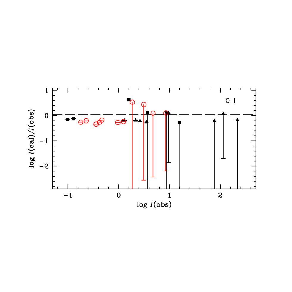
Figure 6: Same as in Fig. 5 for O i lines.

5.8 O i

The triplet terms are excited by fluorescence in the PDR of IC 418 through a large number of resonant transitions of comparable strength from the ground term $\rm 2p^{2}\ {}^{3}P$, a situation also encountered in Orion by Lucy (2002). Triplet O i line profiles shown by SBW are similar to those of the O i forbidden lines in support of the fluorescence excitation mechanism. The quintets on the other hand are produced in the ionized region by recombination of $\rm O^{+}$ with no contribution from fluorescence because they are not connected with strong transitions from the ground term and recombination preferentially populates higher multiplicity states.

SWBH identified several multiplets between terms $\rm 3p\ ^{3}P$ and $\rm 3p\ ^{5}P$ and s states with principal quantum number $n=5$ to 8 and d states with principal quantum number $n=4$ to 7. SBW does not list them although their identifications seem certain and only their effective recombinations are lacking in (Pequignot et al.1991). The effective recombination coefficients for those terms were calculated by Escalante & Victor (1992). Our calculations tend to underestimate systematically the quintet and some triplet intensities by a factor of 1.3, which is slightly higher than the assumed uncertainty and suggests that the effective recombination coefficients of Escalante & Victor (1992) may be underestimated. The effective recombination coefficients of (Pequignot et al.1991) are higher by about that same factor, and thus give a closer agreement with the observations.

The forbidden lines of the ground configuration $\rm 2p^{4}\ {}^{3}P_{2}$–$\rm 2p^{4}\ {}^{1}D_{2}$$\lambda\,$6300.30, $\rm 2p^{4}\ {}^{3}P_{1}$–$\rm 2p^{4}\ {}^{1}D_{2}$$\lambda\,$6363.78 and $\rm 2p^{4}\ {}^{1}D_{2}$–$\rm 2p^{4}\ {}^{1}S_{1}$$\lambda\,$5577.34 are excited by electron collisions with negligible contribution from fluorescence in the warm interface of the PDR and ionized region. Our predicted intensities for those lines are underestimated by the same amount as the recombination lines, but they are more sensitive to the density than the N i optical forbidden lines. If the $n_{3}$ parameter in equation (7) is raised to 35000, our predicted intensities of the three forbidden lines perfectly match the observed values. This value of the density is already too high to explain the FIR [C ii] and [O i] line observations of Liu et al. (2001a). It is also possible to improve the agreement of the calculated fluorescence and recombination lines with the measurements if the PDR were larger, but there is no evidence of a dense and extended neutral medium around IC 418. Such a medium would increase the FIR line fluxes beyond their observed uncertainty.

The largest discrepancy with the observations occurs in multiplet $\rm 3p\ ^{3}P_{0,1,2}$–$\rm 5s\ ^{3}S^{o}_{1}$$\lambda\,$7254.15–.53 with an observed intensity 1.8 times the predicted one. The possibility of an overestimated observed intensity due to a low S/N (Rola & Pela, 1994) can be ruled out because the S/N measured by SWBH for the $\lambda\,$7254 multiplet is 15.0. There is only one O i line with $\rm S/N<7$ in our calculations. Most of the O i lines or blends are relatively intense with $\rm S/N>100$. Lines from other states in the Rydberg series, $\rm 6s\ ^{3}S^{o}_{1}$, and $\rm 8s\ ^{3}S^{o}_{1}$ agree better with the calculated values.

SWBH also identified the feature at $\lambda\,$4654.475 as the O i multiplet $\rm 3p\ ^{5}P_{2}$–$\rm 8d\ ^{5}D^{o}_{1,2,3}$≲4654.56, which is strongly underestimated by a factor of 11 in our calculations and is not listed in table 14. We notice that the other terms in the series $\rm 6d\ ^{5}D$ and $\rm 7d\ ^{5}D$ were not detected by SWBH. For example, the other multiplets in the Rydberg series, $\rm 3p\ ^{5}P_{2}$–$\rm 6d\ ^{5}D^{o}_{1,2,3}$ at $\lambda\,$4967.88 and $\rm 3p\ ^{5}P_{2}$–$\rm 7d\ ^{5}D^{o}_{1,2,3}$ at $\lambda\,$4772.91 should be theoretically stronger by 2.3 and 1.4 times the intensity of the $\lambda\,$4654.56 multiplet respectively according to the recombination rates of Escalante & Victor (1992), and should be above the noise in their respective parts of the spectrum. As noted in section 5.4, an identification as a N ii line is more likely, and therefore the line at $\lambda\,$4654.56 is probably a misidentification as a O i line.

5.9 Variation of the SED

We compared results calculated with the original SED of MG and the new SED described in section 4.1 to gauge the dependence of the fluorescence excitation on theoretical assumptions about the stellar atmosphere.

With few exceptions, most of the variation in results occurs in the N ii lines because of their high fluorescence excitation. The new SED increases the intensities of some N ii lines from p states by 25 per cent and the lines originating in the $\rm 3d\ ^{3}D^{o}_{2}$ state by a factor of 2. The only significant decrease is a factor of 2 in the line $\rm 3p\ ^{3}D_{1}$–$\rm 3d\ ^{3}P^{o}_{0}$$\lambda\,$4459.937. We traced back the cause of those variations to an increase of the stellar flux in the new SED at the wavelength of the transition $\rm 2p^{2}\ {}^{3}P_{2}$–$\rm 3d\ ^{3}D^{o}_{2}$$\lambda\,$533.815, and a decrease at the wavelength of the transition $\rm 2p^{2}\ {}^{3}P_{1}$–$\rm 3d\ ^{3}P^{o}_{0}$$\lambda\,$529.413, which pump the observed lines. Minor variations occur in N ii singlet lines $\rm 3p^{1}P_{1}$–$\rm 3d^{1}D^{o}_{2}$$\lambda\,$4447.03 and $\rm 3p^{1}D_{2}$–$\rm 3d^{1}F^{o}_{3}$$\lambda\,$6610.56, which are strongly excited by fluorescence.

6 Summary

We have calculated the intensities of weak emission lines of C ii, N i, N ii, O i and O ii using a consistent nebular model and SED, which proved successful in previous work in reproducing the intense emission lines and overall density diagnostics and surface brightness maps of IC 418. We compared our calculations with a published deep spectroscopic survey taking into account the fine structure of the lines and including some weak lines with possible blends. Although this nebula shows an almost spherical symmetry, our calculations do take into account the position, size and orientation of the aperture used in the observations.

As in our previous work on the Orion nebula, we found that fluorescence is responsible for the excitation of lines from s, p and d states in N ii. Fluorescence also contributes significantly to the excitation of most lines of the s, p and d states in C ii and some p and d states of O ii while the rest of the O ii states are mostly excited by recombination. Some lines excited by fluorescence are sensitive diagnostics of the details of the SED, the expansion velocity gradient and turbulence of the nebula, the transition probabilities involved in the pumping mechanism, and their intensity is closely related to lines in the stellar atmosphere. The recombination rates can explain most of the observed intensities from f and g states of all species in the ionized region although there are many observed transitions with excited core configurations awaiting the calculation of their effective recombination coefficients.

Ionic abundances deduced from dipole–allowed lines assuming pure recombination rates without taking into account fluorescence excitation of the lines can be overestimated by factors of up to 10 for C ii, 200 for N ii, 2 for O ii, and 500 for N i and O i depending on the transition being considered, and a detailed nebular model and SED are needed to properly estimate ionic abundances from lines mostly excited by fluorescence.

The automated procedure of line identification with the emili code seems to be in accordance with our calculations because the largest discrepancies between predicted and observed line intensities tend to occur in lines with dubious identifications or blends as indicated by that code. A deep spectroscopic nebular survey coupled with an appropriate line identification procedure can prove useful to test the accuracy of quantum mechanical calculations of atomic data.

The N i quartet and O i triplet lines are produced by fluorescence in a narrow and dense interface of the neutral and ionized regions. Electron collisions compete with fluorescence in the excitation of the [N i]$\lambda\,$5200.26 and $\lambda\,$5197.90 lines while fluorescence contributes a negligible amount to the excitation of the [O i]$\lambda\,$6300.30, 6363.78 and $\lambda\,$5577.34 lines. However our calculations tend to underestimate systematically the observed intensities of the [N i] lines by a factor of 5, and further work on the modeling of the PDR is necessary to fully understand the formation of those lines.

References

- (1) Abrahamsson E., Krems R. V., Dalgarno A., 2007, ApJ, 654, 1171
- Allen (1973) Allen C. W., 1973, Astrophysical Quantities, 3rd ed., §27, London: The Athlone Press.
- Baldwin et al. (2000) Baldwin J. A., Verner E. M., Verner D. A., Ferland G. J., Martin P. G., Korista K. T., Rubin R. H., 2000, ApJS, 129, 229
- Bautista (1999) Bautista M. A., 1992, ApJ, 527, 474
- Bell et al. (1995) Bell K. L., Hibbert A., Stafford R. P., McLaughlin B. M., 1995, Physica Scripta, 50, 343
- (6) Bell K. L., Berrington K. A., Thomas M. R. J., 1998, MNRAS, 293, L83
- Berrington & Burke (1981) Berrington K. A., Burke P. G., 1981, Planet. Space Sci., 29, 377
- Cohen & Barlow (1974) Cohen M., Barlow M. J., 1974, ApJ, 193, 401
- (9) Davey A. R., Storey P. J., Kisielius R., 2000, A&A Suppl., 142, 85
- Dayal & Bieging (1996) Dayal A., Bieging J. H., 1996, ApJ, 472, 703
- Ercolano (2009) Ercolano B., 2009, MNRAS, 397, L69
- Escalante (2002) Escalante V., 2002, RMAA (Serie de Conferencias), 12, 22
- Escalante & Góngora–T. (1990) Escalante V., Góngora–T. A., ApJS, 74, 819
- Escalante and Morisset (2005) Escalante V., Morisset C., 2005, MNRAS, 361, 813 (EM)
- Escalante & Victor (1990) Escalante V., Victor G. A., 1990, ApJS, 73, 513 (EV)
- Escalante & Victor (1992) Escalante V., Victor G. A., 1992, Planet. Space Sci., 40, 1705
- Escalante & Victor (1994) Escalante V., Victor G. A., 1994, At. Data Nuc. Data Tables, 56, 213
- Esteban et al. (1998) Esteban C., Peimbert M., Torres–Peimbert S., Escalante V., 1998, MNRAS, 295, 401
- Esteban et al. (2004) Esteban C., Peimbert M., García–Rojas J., Ruiz M. T., Peimbert A., Rodríguez M., 2004, MNRAS, 355, 229
- (20) Fang X., Storey P. J., Liu X.–W. 2011, A&A, 530, A18 (FSL)
- Ferland (1992) Ferland G. J., 1992, ApJ Letters, 389, L63
- Ferland et al. (1998) Ferland G. J., Korista K. T., Verner D. A., Ferguson J. W., Kingdon J. B., Verner E. M., 1998, PASP, 110, 761
- Froese Fischer & Tachiev (2004) Froese Fischer C., Tachiev G., 2004, Atomic Data and Nuclear Data Tables, 87, 1
- García–Rojas & Esteban (2007) García–Rojas J., Esteban C., 2007, ApJ, 670, 457
- (25) García–Rojas J., Peña M., Peimbert A., 2009, A&A, 496, 139
- Gesicki et al. (1996) Gesicki K., Acker A., Szczerba R., 1996, A&A, 309, 907
- Goldbach et al. (1992) Goldbach C., Lüdthe T., Martin M., Nollez G., 1992, A&A, 266, 605
- Grandi (1975) Grandi S. A., 1975, ApJ, 196, 465
- Grandi (1976) Grandi S. A., 1976, ApJ, 206, 658
- Gussie el al. (1995) Gussie G. T., Taylor A. R., Dewdney P. E., Roger R. S., 1995, MNRAS, 273, 790
- Hibbert et al. (1991) Hibbert A., Biemont E., Godefroid M., Vaeck N., 1991, A&A Suppl., 88, 505
- Hillier & Miller (1998) Hillier D. J., Miller D. L., 1998, ApJ, 496, 407
- (33) Hora J. H., Latter W. B., Deutsch L. K., 1999, ApJS, 124, 195
- Howarth & Prinja (1968) Howarth I. D., Prinja R. K., 1989, ApJS, 69, 527
- Huggins et al. (1996) Huggins P. J., Bachiller R., Cox P., Forveille T., 1996, A&A, 315, 284
- Hummer & Storey (1992) Hummer D. G., Storey P. J., 1992, MNRAS, 254, 277
- Khriplovich & Matvienko (2007) Khriplovich I. B., Matvienko D. V., 2007, Physics Letters A, 368, 348
- Kafatos & Lynch (1990) Kafatos M., Lynch J. P., 1990, ApJS, 42, 611
- (39) Krems R. V., Jamieson M. J., Dalgarno A., 2006, ApJ, 647, 1531
- (40) Lavín C., Olalla E., Martín I., 2000, ApJ543, 1051
- Liu et al. (1995) Liu X.–W., Storey P. J., Barlow M. J., Clegg R. E. S., 1995, MNRAS, 272, 369
- Liu et al. (2001a) Liu X.–W., Barlow M. J., Cohen M., Danziger I. J., Luo S.–G., Baluteau J. P., Cox P., Emery R. J., Lim T., Péquignot D., 2001, MNRAS, 323, 343
- Liu et al. (2001b) Liu X.–W., Luo S.–G., Barlow M. J., Danziger I. J., Storey P. J., 2001, MNRAS, 327, 141
- Liu et al. (2006) Liu X.-W., Barlow M. J., Zhang Y., Bastin R. J., Storey P. J., 2006, MNRAS, 368, 1959
- Lucy (2002) Lucy L. B., 2002, MNRAS, 329, 787
- (46) Luo S.–G., Liu X.–W., Barlow M. J., 2001, MNRAS, 326, 1049
- Luridiana et al. (2009) Luridiana V., Simón-Díaz S., Cerviño M., González Delgado R. M., Porter R. L., Ferland G. J., 2009, ApJ, 691, 1721
- Mar et al. (2000) Mar S., Pérez G., González V. R., Gigosos M. A., del Val J. A., de la Rosa I., Aparicio J. A., 2000, A&A Suppl., 144, 509
- Meixner et al. (1996) Meixner M., Skinner C. J., Keto E., Zijlstra A., Hoare M. G., Arens J. F., Jernigan J. G., 1996, A&A, 313, 234
- (50) Mesa–Delgado A., Esteban C., García–Rojas J., 2008, ApJ675, 389
- (51) Monk D. J., Barlow M. J., Clegg R. E. S., 1990, A&A, 242, 457
- Morisset (2006) Morisset C., 2006 in IAU Symposium, Vol. 234., Planetary Nebula in our Galaxy and Beyond, ed. M. J. Barlow & R. H. Méndez, p. 467
- Morisset & Georgiev (2009) Morisset C., Georgiev L., 2009, A&A, 507, 1517 (MG)
- Morisset & Stasińska (2006) Morisset C., Stasińska G., 2006, RMAA, 42, 153 (MG)
- Nahar (1995) Nahar S. N., 1995, ApJS, 101, 423
- Nahar (2009) Nahar S. N., 2010, Atomic Data and Nuclear Data Tables, 96, 863
- Neiner et al. (1996) Neiner, C., Acker A., Gesicki K., Szczerba R., 2000, A&A, 358, 321
- Nussbaumer & Storey (1981) Nussbaumer H., Storey P. J., 1981, A&A, 96, 91
- Nussbaumer & Storey (1984) Nussbaumer H., Storey P. J., 1984, A&A Suppl., 56, 293
- Otsuka et al. (2009) Otsuka M., Hyung S., Lee S.–J., Izumiura H., Tajitsu A., 2009, ApJ, 705, 509
- (61) Péquignot D., Petitjean P., Boisson C., 1991, A&A, 251, 680
- (62) Ralchenko Yu., Kramida A. E., Reader J., and NIST ASD Team, 2008, NIST Atomic Spectra Database (version 3.1.5), in electronic form at http://physics.nist.gov/pml/data/asd.cfm, National Institute of Standards and Technology, Gaithersburg, MD.
- Rola & Pela (1994) Rola, C., Pela D., 1994, A&A, 287, 676
- Sharpee et al. (2003) Sharpee B., Williams R., Baldwin J. A., van Hoof P. A. M., 2003, ApJS, 149, 157 (SWBH)
- (65) Sharpee B., Baldwin J. A., Williams R., 2004, ApJ, 615, 323 (SBW)
- Seaton (1959) Seaton M. J. 1959, MNRAS, 119, 70
- Seaton (1968) Seaton M. J. 1968, MNRAS, 139, 129
- Seaton et al. (1994) Seaton M. J., Yan Y, Mihalas D., Pradhan A. K., 1994, MNRAS, 266, 805
- (69) Shen X.–Z, Yuan P., Liu J., 2010, Chinese Physics B, 19, 053101
- Storey (1994) Storey P. J., 1994, A&A, 282, 999
- Tayal (2006) Tayal A. R., 2006, ApJS, 163, 207
- Taylor & Pottasch (1987) Taylor A. R., Pottasch S. R., 1987, A&A, 176, L5
- (73) Taylor A. R., Gussie G. T., Goss W. M., 1989, ApJ, 340, 932
- (74) Torres–Peimbert S., Peimbert M., Daltabuit E., 1980, ApJ, 238, 133
- Tsamis et al. (2008) Tsamis Y. G., Walsh J. R., Péquignot D., Barlow M. J., Danziger I. J., Liu X.–W., 2008, MNRAS, 2008, 386, 22
- Veres & Wise (1996) Veres G., Wise W. L., 1996, Phys. Rev. A, 54, 1999.
- Victor & Escalante (1988) Victor G. A., Escalante V., 1988, Atomic Data and Nuclear Data Tables, 40, 227
- Viegas & Clegg (1994) Viegas S. M., Clegg R. E. S., 1994, MNRAS, 271, 993
- Wen & O’Dell (1995) Wen Z., O’Dell C. R., 1995, ApJ, 438, 784
- Wenåker (1990) Wenåker I., 1990, Physica Scripta, 42, 667
- (81) Wesson, R., Stock, D. J., Scicluna, P., 2012, MNRAS, 422, 3516
- (82) Wiese W. L., Fuhr J. R., Deters T. M., 1996, Atomic Transition Probabilities of Carbon, Nitrogen, and Oxygen, Journal of Physical Chemical Reference Data Monograph No. 7, New York: American Chemical Society
- Williams et al. (2008) Williams R., Jenkins E. B., Baldwin J. A., Zhang Y, Sharpee B, Pellegrini E., Phillips M., 2008, ApJ, 677, 1100
- (84) Yan Y., Taylor K. T., Seaton M. J., 1987, J. Phys. B, 20, 6399
- Zhang (2008) Zhang Y., 2008, A&A, 486, 221