Critical Behavior of the Three-Dimensional Ising model with Anisotropic Bond Randomness at the Ferromagnetic-Paramagnetic Transition Line

Abstract

We study the $\pm J$ three-dimensional Ising model with a spatially uniaxially anisotropic bond randomness on the simple cubic lattice. The $\pm J$ random exchange is applied in the $xy$ planes, whereas in the z direction only a ferromagnetic exchange is used. After sketching the phase diagram and comparing it with the corresponding isotropic case, the system is studied, at the ferromagnetic-paramagnetic transition line, using parallel tempering and a convenient concentration of antiferromagnetic bonds ($p_{z}=0;p_{xy}=0.176$). The numerical data point out clearly to a second-order ferromagnetic-paramagnetic phase transition belonging in the same universality class with the 3d random Ising model. The smooth finite-size behavior of the effective exponents describing the peaks of the logarithmic derivatives of the order parameter provides an accurate estimate of the critical exponent $1/\nu=1.463(3)$ and a collapse analysis of magnetization data gives an estimate $\beta/\nu=0.516(7)$. These results, are in agreement with previous studies and in particular with those of the isotropic $\pm J$ three-dimensional Ising at the ferromagnetic-paramagnetic transition line, indicating the irrelevance of the introduced anisotropy.

I Introduction

Ising spin glass models yield phase diagrams with distinctively complex ordered phases, in $d=3$. These models, although relatively simple in their formulation, have been proposed to describe complex systems exhibiting frustration, e.g., materials such as ${\mathrm{Fe_{1-xi}Mn_{xi}TiO_{3}}}$ and ${\mathrm{Eu_{1-x}Ba_{x}MnO_{3}}}$ glass-metal ; glass-metal2 ; glass-metal3 , neural networks hopfield1 etc.

The simplest of such models, but most influential over the years, is the Edwards Anderson model ea-model ; BindY86 defined by the Hamiltonian

$$H=-\sum_{\langle ij\rangle}J_{ij}s_{i}s_{j},$$ (1)

where the summation is over nearest-neighbors, $s=\pm 1$ and $J_{ij}$ denotes the uncorrelated quenched exchange interaction. There are two popular quenched random disorder distributions, the Gaussian distribution of random bonds with zero mean and unity standard deviation and the bimodal distribution of $J_{ij}$ given by

$$P(J_{ij})=p\delta(J_{ij}+1)+(1-p)\delta(J_{ij}-1)$$ (2)

Recently, the spatially uniaxially anisotropic $d=3$ spin glass system has been solved exactly on a hierarchical lattice by Guven et al. anis_1 . Their general study revealed a rich phase diagram topology and several new interesting features. The Hamiltonian of this anisotropic variant, differentiates, along $z$ axis, the probability distribution of quenched randomness, but also the strength of the exchange interaction and can be written

$$H=-\sum_{u}\sum_{\langle ij\rangle_{u}}J_{ij}^{u}s_{i}s_{j},$$ (3)

Accordingly, the bimodal distribution of $J_{ij}^{u}$ takes the more general form

$$P(J_{ij}^{u})=p_{u}\delta(J_{ij}^{u}+J^{u})+(1-p_{u})\delta(J_{ij}^{u}-J_{ij}^{u})$$ (4)

where $u$ denotes the $z$ axis $(u=z)$ or the $xy$ planes $(u=xy)$, $J_{ij}^{u}$ denote the corresponding exchange interactions and $p_{u}$ are the probabilities of two neighboring spins ($ij$) having antiferromagnetic interaction along $z$ axis or the $xy$ planes.

The standard isotropic case, defined by Eq. (1) and Eq. (2), corresponds to $J_{ij}^{z}=J_{ij}^{xy}$ and $p_{z}=p_{xy}$. The global phase diagram of this isotropic case, is sketched in Fig. 1 and, as shown, there exist (in $d=3$) three distinctive phases, ferromagnetic, paramagnetic and glassy phases. All transitions among these phases, are believed to be of second order and also to belong to different universality classes. Several accurate studies have been carried out, to determine the critical behaviors along these transition lines, for the finite-temperature phase transitions FG_1 ; hasen_fp ; hasen_sg ; katz_pg ; jorg ; campb_sg ; balle_sg ; pala_sg ; kawa_is ; bill-11 . Most of these studies concern the ferromagnetic-paramagnetic (FP) and the glassy-paramagnetic (GP) lines. There is also a recent study for the ferromagnetic-glassy transition line FG_1 . The transition lines meet in a multicritical point hasen_mcp ; mcp_2d ; ozeki-ito ; mcp_2 ; doussal_harris_1 ; doussal_harris_2 located along the Nishimory line  nishimori_book ; nishimori_1980 ; nishimori_1981 ; nishimori_1986 with coordinates $T_{M}=1.6692(3),p_{M}=0.23180(4)$ hasen_mcp ; mcp_2d ; ozeki-ito ; mcp_2 . The FP transition line, starts at the pure Ising model ($p=0$), for which all critical properties have been extensively studied and a recent very accurate estimate of the correlation length exponent is $\nu=0.63002(10)$ Hase10 ; camp_is ; guida_is ; Butera-02 with a critical temperature $T_{c}=4.5115232(16)$  Hase10 ; camp_is ; guida_is ; Butera-02 ; deng_is ; blote_is . As shown by Hasenbusch et al. hasen_fp , the introduction of the $\pm J$ quenched randomness changes the universality of the model to that of the random Ising model (RIM) or randomly diluted Ising model (RDIs) kawa_is ; hukushima_fp ; hasen_fp , in which several spin models appear to belong. These, include models such as the randomly site and bond diluted, the random bond  balles_rdi ; hasen_rdi ; pelis_rdi ; berche-04 ; theod_fytas , the random bond Blume-Capel mal_3drbc model and, of course, the already mentioned isotropic $\pm J$ three-dimensional Ising at the ferromagnetic-paramagnetic transition line hasen_fp . An accurate estimate of the correlation length exponent for these $d=3$ FP transitions, characterizing the RIM universality class, is that given by  balles_rdi $\nu=0.6837(53)$.

For the glassy-paramagnetic (GP) transition line ($MB$ line in  Fig.1), most of the work has been curried out at $p=\frac{1}{2}$  ogiel-85 ; ogiel-85-2 ; sing_sg ; bhatt_sg ; kawa_young ; bern_sg ; berg_sg ; pala_sg ; mari_sg ; balle_sg ; mari_sg-2 ; mari_sg-3 ; naka_sg ; pleim_sg ; campb_sg ; campb_sg-2 ; katz_pg . However, because of severe inherent difficulties, due to both strong frustration and disorder effects in this region, there is a large spread in the estimates of critical exponents and there remain some questions related to universality. This is very clearly reflected in Table I of Katzgraber et al. katz_pg in which one can observe a very large spread in the correlation length exponent, and even in the estimates of critical temperature. We shall quote from this paper, the estimates $\nu=2.39(5)$ and $T_{c}=1.120(4)$, which apply to the present isotropic $\pm J$ spin-glass model. We will also quote the more recent estimates $\nu=2.45(15)$, $T_{c}=1.109(10)$ hasen_sg . Finally, from the recent work by Ceccarelli et al. FG_1 , we know that the correlation length exponent for the ferromagnetic-glassy (FG) transitions has been estimated to be $\nu=0.96(2)$.

Several other features of the critical behaviors and the global phase diagram are known for the isotropic case. Ground state calculations by Hartmann hartmann_sggs ($p_{A}=0.222(5)$), indicated a reentrant FG transition line. This was nicely verified by the finite temperature study of Ceccarelli et al. FG_1 , since they estimated $p(T=0.5)=0.2271(2)$, predicting the ferromagnetic-glassy transition line to be slightly reentrant. These results are in accordance with the Nishimori expectations nishimori_1980 ; nishimori_1981 that, this line cannot be forward and are also reflected in renormalization-group calculations miglio_1 ; berker-05 ; anis_1 .

Figure 1: (color on line) Phase diagram points (full squares, asterisk, and dot) of the isotropic Edwards-Anderson model are taken from hasen_fp ; hasen_mcp ; katz_pg ; hartmann_sggs . The phase diagram is drawn in solid lines and separates the three phases: ferromagnetic (F), spin-glass (G), and paramagnetic (P). These lines meet at the multicritical full dot point (M). Dash lines (and open symbols) illustrate the phase diagram of the anisotropic model $p_{z}=0,p=p_{xy}$. The open triangles, asterisk and dot points are discussed in more detail in the text. In particular, the full asterisk ($p=0.117$) corresponds to the improved model case of hasen_fp and the open asterisk ($p=p_{xy}=0.176$) to the improved case studied here.

In this paper we will focus on the nature of the FP transition for the anisotropic model described by Eq. (3) and Eq. (4) by considering the particular model case $p_{z}=0;p_{xy}\leq 0.5$ with $J_{ij}^{z}=J_{ij}^{xy}$. The present study is part of a research program to study by Monte Carlo methods the general spatially uniaxially anisotropic $d=3$ spin glass system considered by Guven et al. anis_1 . The main motivation is to provide numerical evidence for the universality question, by investigating possible effects caused, by the introduced anisotropy, on the critical exponents along the three different transition lines. We hope that our attempts may also play some role in future studies and will provide new information for the critical behavior of frustrated systems.

We start by describing our current perception on the global phase diagram of the above anisotropic case. This phase diagram is sketched also in Fig. 1, by the dash lines. As shown, there exist again(in $d=3$) three distinctive phases, ferromagnetic, paramagnetic and glassy phases. The points shown on the FP transition line have been located from the peaks of the magnetic sample-averaged susceptibility for a lattice of size $L=16$. The open asterisk (see also the solid drop lines) on this line indicate a special point corresponding to $p_{xy}^{*}=0.176$. This choice was inspired by the improved model case analyzed by Hasenbusch et al. hasen_fp for the isotropic model (see on the isotopic phase diagram the case with $p^{*}=0.117$ and the corresponding dash drop lines). According, to Hasenbusch et al. hasen_fp for the isotropic case at $p^{*}=0.117(3)$ the leading scaling corrections vanish and this case provides an improved model for accurate exponent estimation. Our quest for a convenient and improved model case for the anisotropic FP transition, directed as to find the phase diagram point corresponding to about the same temperature as the isotropic phase diagram point. As can be seen, by comparing the drop lines, this would suggest the case $p_{xy}^{*}=0.176$. Alternatively, let us try to satisfy the relation $(1-p_{xy}^{*}(T))=1.5(1-p^{*}(T))-0.5$ between the two FP transition lines. This prognostic method assumes that phase diagram points corresponding to the same temperature would have (approximately) the same ratio of ferromagnetic to antiferromagnetic interactions. Putting $p^{*}=0.117(3)$ in this relation, we find $p_{xy}^{*}=0.1755(30)$, which is practically the above value for the anisotropic case. As it will be seen in the sequel, the proposed case $p_{xy}^{*}=0.176$ provides indeed an excellent case and gives, for the anisotropic model, a very accurate estimate of the correlation length exponent($\nu=0.6835(25)$).

The rest of the anisotropic phase diagram (see also the caption of Fig. 1), was mainly constructed on the premise that the above relation may hold approximately for the lines separating the ferromagnetic phase from the other two phases. Thus, applying this prognostic to the point $p(T=0)=p_{A}=0.222(5)$ of the isotropic case, we find that $p_{xy}(T=0)=p_{A_{ani}}=0.333(5)$. Quite remarkably we found from our ground state calculations a value that perfectly verify this prediction. Based on the rather short calculation of ground states on lattices sizes $L=6,8,10$ we found, by a collapse method, $p_{A_{ani}}=0.332(12)$ astonishingly close to the predicted value. After this, the multicritical point for the anisotropic case, shown in Fig. 1 has been placed by a mere application of the above relation giving $p_{M_{ani}}=0.34770(4)$. One should, of course, realize that this prognostic is only an approximation, which could not be expected to apply in the more general case. It is possible that, it is only successful for the present case giving a reasonable approximation for the FP and FG transition lines. To complete our perception of the anisotropic phase diagram, we point out that for the case $p_{z}=0;p_{xy}\leq 0.5$ we found from Monte Carlo simulations a phase diagram point which appears to coincide with the isotopic phase diagram point $B$. For instance, extrapolating the $L=6,8,10$ Binder’s fourth order cumulant crossings of the overlap order parameter we found $T_{B_{ani}}=1.07(4)$, very close to the corresponding estimate of the isotropic case. This finding appears to be a very interesting and physically appealing prediction. A proof that $T_{B_{iso}}=T_{B_{ani}}$ exactly, may also help a better understanding of the general universality question. In closing this discussion, we shall mention that the introduction of anisotropy changes in general the phase diagram and possibly the symmetry of multicritical points, as discussed by Guven et al. anis_1 . These multicritical points, such as in the present model case ($p_{z}=0;p_{xy}\leq 0.5$), do not necessarily obey Nishimori conditions and one can not exclude the possibility of a ferromagnetic-glassy transition line being forward. However, our prognostic method, insist that the present anisotropic FG transition line is reentrant.

The rest of the paper is laid out as follows: In the following subsection we give a description of our numerical approach utilized to derive numerical data for large ensembles of realizations of the disorder distribution and lattices with linear sizes within the range $L\in\{8-44\}$. Then in subsection II.2 the finite-size scaling (FSS) scheme is described in some detail. In Sec. III we present all our FSS attempts, that give good estimates of all critical exponents and verify that the present anisotropic model belongs to the universality class of RIM. Our conclusions are summarized in Sec. IV.

II MONTE CARLO SIMULATIONS AND FINITE-SIZE SCALING SCHEME

II.1 MONTE CARLO METHOD

In the present paper, we shall use our recent approach to disordered systems mal_3drbc , based on a parallel tempering (PT) practice. Our PT protocol will use an adequate number of Metropolis metro53 sweeps of the lattice, as an elementary Monte Carlo step, so that the correlation times of the PT protocol will be, for all temperatures used, very close to $1.0$. We mention here, that parallel tempering, combined with Metropolis algorithm has been used also by Ceccarelli et al. FG_1 in their study of the FG transition. Further, as pointed out by Hasenbusch et al. hasen_fp , in their study of the isotropic case, the Metropolis algorithm may be more effective than cluster dynamics, for intermediate lattice sizes, as a result of frustration effects present in the $\pm J$ models.

Our PT protocol (also our FSS approach) has been described in detail in our recent paper mal_3drbc ; malakis12 and only a brief summary is given here. For the estimation of the critical properties we generate MC data that cover several finite-size anomalies of the finite systems of linear size $L$. The PT approach is carried over to a certain temperature range depending on the lattice size. These temperatures are selected in such a way that the exchange rate is $0.5$, using a practice similar to that suggested in Ref. bittner11 . The appropriate temperature sequences were generated via short preliminary runs in which we apply a simple histogram method Swendsen87 ; Newman99 ; LandBind00 to determine from the energy probability density functions the temperatures, satisfying the above exchange condition bittner11 ; mal_3drbc . The preliminary runs cover several disorder realizations and the average over the temperatures sequences provides us with a protocol with very small variation in the exchange rate condition, as one moves from one realization to the other.

The proposed MC scheme was carefully tested for all lattice sizes before its implementation for the generation of MC data. The tests included the estimation of the MC times necessary for equilibration and thermal averaging process applied to a particular disorder realization, and involved also the observation of running sample-averages of several thermodynamic quantities, such as the magnetic susceptibility, at a temperature close to criticality. Provided we use reasonably long MC times for equilibration and thermal averaging we find an effective cancellation of statistical errors from the sample-averaging process, since the sample-to-sample fluctuations are larger (by an order of magnitude) than the usual statistical errors (in the thermal averaging process).

The present simulation task is, of course, quite considerable, since we have to satisfy both a good equilibration of the system and also sum over a very large number of disorder realizations. The number of realizations influence the accuracy of our data, and the proper selection of temperatures influence their suitability for the locations of the finite-size anomalies. Since we are implementing a PT approach, based on temperatures corresponding to an exchange rate $0.5$, we are selecting proper temperature sequences consisting of a number of (say 3 or 5) different temperatures and averaging for this set of temperatures over a relatively large number ($\sim 1000$) of disorder realizations. This yields a number of (3 or 5) points of the averaged curves $[Z]_{av}$, where $Z$ denote the thermal average of some thermodynamic quantity, such as the magnetic susceptibility. The PT protocol is repeated several times (depending on the linear size $L$) by using new sets of temperatures(translated with respect to the previous sets) and a final dense set of points is obtained. The above is an efficient and most importantly quite accurate practice, since we finally obtain averaged curves corresponding to a very large number of realizations, describing with high accuracy all the averaged finite-size anomalies of the system. Monte carlo data were collected for systems of linear sizes $L={8,12,16,20,24,28,32,36,40,44}$ and the FSS analysis was performed to the averaged quantities obtained from these MC data.

II.2 FINITE-SIZE SCALING SCHEME

In the standard approach of FSS for a random system, a large number of disorder realizations has to be used in the summations in order to obtain good sample-averages of the basic thermodynamic quantities $Z$, which are the usual thermal averages of a single disorder realization. From the disorder averages $[Z]_{av}$ we obtain their finite-size anomalies, denoted here as $[Z]_{av}^{\ast}$. These finite-size anomalies will be used in our FSS attempts, following a quite common practice chate-01 . Their temperature locations, denoted by $T_{[Z]_{av}^{\ast}}$ will be used in the sequel in our FSS attempts. Thus, our study concerns the critical exponents describing the disorder-averaged behavior and we do not attempt a FSS analysis based on sample dependent pseudocritical temperatures. The later is, a more demanding alternative approach wiseman-98 ; DSFish95 ; Chay86 , which considers the individual sample dependent maxima (anomalies) and the corresponding sample dependent pseudocritical temperatures. Note that, for disordered systems one could make in principle a clear distinction between typical and averaged exponents DSFish95 ; Chay86 .

From the MC data, several pseudocritical temperatures may be estimated, corresponding to finite-size anomalies and these are expected to follow a power-law shift behavior $T_{[Z]_{av}^{\ast}}=T_{c}+b_{Z}\cdot L^{-1/\nu}$. The traditionally used specific heat and magnetic susceptibility peaks, as well as the peaks corresponding to the following logarithmic derivatives of the powers $n=1$, $2$, and $n=4$ of the order parameter with respect to the inverse temperature $K=1/T$ ferrenberg91 ,

$$\frac{\partial\ln\langle M^{n}\rangle}{\partial K}=\frac{\langle M^{n}H\rangle}{\langle M^{n}\rangle}-\langle H\rangle,$$ (5)

and the peak corresponding to the absolute order-parameter derivative

$$\frac{\partial\langle|M|\rangle}{\partial K}=\langle|M|H\rangle-\langle|M|\rangle\langle H\rangle,$$ (6)

will be located and used in our fitting attempts.

The behavior of the maxima of the logarithmic derivatives of the powers $n=1$, $2$, and $n=4$ of the order parameter with respect to the inverse temperature, which as is well known scale as $\sim L^{1/\nu}$ with the system size ferrenberg91 , will be seen to provide a smooth root for the estimation of the correlation length exponent $\nu$. Once the exponent $\nu$ is well estimated, the behavior of the values of the peaks corresponding to the absolute order-parameter derivative, which scale as $\sim L^{(1-\beta)/\nu}$ with the system size ferrenberg91 , gives one route for the estimation of the magnetic exponent ratio $\beta/\nu$.

For the estimation of the critical temperature, we shall use mainly a simultaneous fitting approach of the several pseudocritical temperatures mentioned above. However, from the MC data for the disorder averaged magnetization, it is possible to follow an optimum collapse method which will provide simultaneously estimates for the critical exponents $\beta/\nu,{1/\nu}$ as well as the critical temperature $T_{c}$. From the scaling hypothesis

$$[\langle|M|\rangle]_{av}=M(T,L)=L^{-\beta/\nu}{f}[(T-T_{c})L^{1/\nu}],$$ (7)

and the disorder averaged magnetization data, we attempt in the next section the estimation of critical behavior by using a recently published collapse method that makes use of the downhill simplex algorithm collapse .

III ESTIMATION OF CRITICAL BEHAVIOR

As pointed out earlier, the present study uses the finite-size anomalies of the sample average of the logarithmic derivatives of the powers ($n=1,2,4$) of the order parameter with respect to the inverse temperature, for the estimation of the correlation length exponent $\nu$. It will be seen that, the finite size scaling behavior of the corresponding peaks provides for the present model an attractive and smooth approach to this estimation. Assuming that these finite-size anomalies ($[Z]_{av}^{\ast}$) of the disorder averages $[Z]_{av}$, where $Z$ is the thermal average given by Eq. (5), scale as $\sim L^{1/\nu}$ with the system size ferrenberg91 we estimate in figures  2 and  3 this exponent. A very good scaling behavior is observed already by using the whole size range of our Monte carlo data $L=[8-44]$. The simultaneous fitting attempt to the expected power-law behavior, illustrated in Fig. 2, gives the estimate shown in the panel: ${1}/\nu=1.468(6)$.

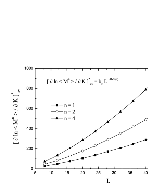
Figure 2: (color online) FSS behavior of the peaks of the logarithmic derivatives of the powers $n=1$, $2$, and $n=4$ of the order parameter with respect to the inverse temperature. The estimate for the exponent $1/\nu=1.468(6)$ (shown in the panel) is obtained by applying a simultaneous fitting attempt to a simple power law in the whole size range $L=8-44$.

By varying the $L_{min}$, in these simultaneous fitting attempts, we obtain a sequence of effective exponents depending on the minimum size used. The behavior of these effective exponents is shown in Fig. 3. The smooth, almost perfectly linear, behavior of these effective exponents enables us to estimate confinedly ${1}/\nu=1.463(3)$. The error range of this estimation is indicated in Fig. 3 by the dot lines and is compared with the corresponding 3d pure Ising model for which an extremely accurate estimation is availableHase10 . The present estimate for the correlation length exponent $\nu=0.6835(25)$, compares well with the estimate $\nu=0.683(3)$ of Hasenbusch et al. hasen_fp , for the corresponding isotropic $\pm J$ Ising model at the ferromagnetic-paramagnetic transition line and is in excellent agreement with the estimate $\nu=0.6837(53)$, of the extensive numerical investigations of Ballesteros et al. balles_rdi for the site-diluted Ising model. The good behavior of the effective exponents in Fig. 3, giving improved error bounds, suggest the present model as a suitable candidate for further attempts and refinements of this exponent, possibly following the more sophisticated approach of Hasenbusch et al. hasen_fp to extend the Monte Carlo data to larger lattice sizes.

Figure 3: (color online) Illustration of the behavior of the effective exponents $(1/\nu)_{eff}$. The solid line drawn in the panel, together with the dot lines, indicate the critical exponent range for the present model. The linear behavior illustrated give the accurate estimation $1/\nu=1.463(3)$. For comparison the analogous narrow range $1/\nu=1.587(1)$ Hase10 , for the pure 3d Ising model is shown in the upper part of the panel.

We proceed to calculate the critical exponent ratio $\gamma/\nu$ from the peaks of the sample-averaged susceptibility ($[\chi]_{av}^{\ast}$). We assume that these finite-size anomalies obeys a simple power law: $[\chi]_{av}^{\ast}=b\cdot L^{\gamma/\nu}$, and follow again the practice of observing the behavior of effective exponents by varying the $L_{min}$ of the fitting range. The resulting sequence of effective exponents ($L_{min}=[8-24]$) is illustrated in Fig. 4. As seen from this figure, the behavior of these estimates is not linear. Thus, the attempted linear fit, appears as an overestimation, but gives clearly the underestimated estimate $\gamma/\nu=1.9614(28)$, appreciably smaller than that of Ballesteros et al. balles_rdi $\gamma/\nu=1.963(5)$ and even more than those of Hasenbusch et al. $1.964(1)$ hasen_rdi for the site-diluted 3d Ising model and $1.964(2)$ hasen_fp for the corresponding to the present model isotropic $\pm J$ Ising model at the ferromagnetic-paramagnetic transition line. Therefore, the estimation via the susceptibility peaks is here unsatisfactory.

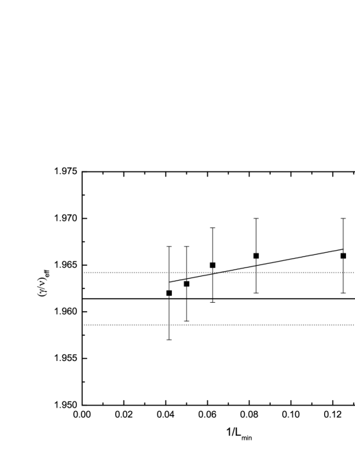
Figure 4: (color online) Illustration of the behavior of the effective exponents $\gamma/\nu$. The solid line drawn in the panel, together with the dot lines, indicate the unsatisfactorily estimated critical exponent range $\gamma/\nu=1.9614(28)$.

We may now attempt the estimation of the exponent ratio $\beta/\nu$, via the scaling behavior of the peaks corresponding to the absolute order-parameter derivative which is expected to scale as $[\partial\langle|M|\rangle/\partial K]_{av}^{\ast}=b\cdot L^{(1-\beta)/\nu}$. The corresponding effective exponent estimates, illustrated in Fig. 5, show again a behavior which, as seen, is not linear. The illustrated in the figure linear fit gives ${(1-\beta)/\nu}=0.9572(54)$, which by using our estimate $1/\nu=1.463(3)$, produces for $\beta/\nu$ the range $0.5058(84)$. However, this value is noticeably smaller than the value $\beta/\nu=0.518$, expected from hyperscaling and accepting an estimate for $\gamma/\nu$ of the order of the above mentioned literature estimates (say for instance: $\gamma/\nu=1.964$). The situation in this case can be improved by attempting the linear fit in Fig. 5 only at the last three points. The linear fit in these three points ($L_{min}=16,20,24$), gives ${(1-\beta)/\nu}=0.948(3)$ producing, as above, $\beta/\nu=0.515(6)$. Note also, that the second order polynomial fit, shown also in Fig. 5 and applied to all five points, gives an estimate ${(1-\beta)/\nu}=0.943(6)$ producing now $\beta/\nu=0.520(9)$. These values are in good accordance with hyperscaling and the literature estimate of $\gamma/\nu$.

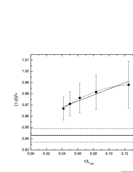
Figure 5: (color online) Illustration of the behavior of the effective exponents $(1-\beta)/\nu$. The solid and the dash lines drawn through the points indicate linear and second-order polynomial fits, discussed in the text. The critical exponent range for the later fit is indicated by the heavy solid and dot lines at $(1-\beta)/\nu=0.943(6)$.

The critical temperature will be now estimated by a simultaneous fitting approach, using several pseudocritical temperatures of the sample average of the quantities measured malakis09 ; malakis12 , as outlined earlier. The simultaneous fitting is attempted to the expected power-law shift behavior $T_{[Z]_{av}^{\ast}}=T_{c}+b_{Z}\cdot L^{-1/\nu}$ for the six pseudocritical temperatures mentioned in the previous section.

Figure 6: (color online) Illustration of the behavior of the effective pseudocritical temperatures obtained by applying a simultaneous fit on the shift behavior $T_{[Z]^{*}}=T_{c}+b_{Z}L^{-1/\nu}$ and fixing the exponents to the accurate estimate $1/\nu=1.463$. The solid dot lines indicate the critical temperature range $T_{c}=3.2931(12)$ obtained by the illustrated linear fit.

We approach this estimation by simultaneous fittings in which we are fixing the exponent $1/\nu$ to the apparently accurate estimate $1/\nu=1.463$. Following our earlier practice of using different fitting ranges by varying the $L_{min}$ of the fitting range, we obtain a sequence of estimates illustrated in Fig.6. The linear fit shown in the panel gives an estimate $T_{c}=3.2931(12)$ illustrated with solid and dot lines in this figure, whereas restricting the fit only to the last three points, corresponding to $L_{min}=16,20,24$, gives a higher estimate $T_{c}=3.2945(18)$. We note here that a completely free fit, without fixing any parameter, and following the above practice gives $T_{c}=3.2934(8)$ from the linear fit to the five points $L_{min}=8,12,16,20,24$ and $T_{c}=3.2940(16)$ from the linear fit to the three points $L_{min}=16,20,24$. Thus, we will suggest that $T_{c}=3.2938(9)$

Figure 7: (color online) Illustration of magnetization data collapse for lattice sizes $L={12-44}$. The method used is discussed in detail in the text and gives as shown in the panel an optimum collapse at the values $T_{c}=3.2928(7)$, $1/\nu=1.466(12)$, and $\beta/\nu=0.516(7)$.

Finally, we present the alternative estimation of critical behavior by studying the expected scaling law Eq. (7) for the order parameter data, here the disorder averaged magnetization data. Using the earlier mentioned collapse method, we rescale the $y$ axis to $ML^{\beta/\nu}$ and the $x$ to $(T-T_{c})L^{1/\nu}$, and we attempt to observe the optimum collapse of the magnetization curves taken from different lattice sizes ($L=[12-44]$). We apply the downhill simplex algorithm as developed and implemented in reference collapse for the estimation of critical properties and their error bounds. As shown in the panel of Fig.7, the optimum collapse gives $\beta/\nu=0.516(7)$. This value is in very good agreement with the expected value as mentioned earlier. In the panel we also give, the resulting estimates for the exponent $1/\nu=1.466(12)$ and the estimate for the critical temperature $T_{c}=3.2928(7)$. These are in fair agreement with our previous findings. However, the estimate $\beta/\nu=0.516(7)$, appears to be very satisfactory.

IV Conclusions

The present paper pointed out clearly that, the $\pm J$ three-dimensional Ising model, with spatially uniaxially anisotropic bond randomness, give rise to a second-order phase transition belonging in the same universality class with the 3d random Ising model. The implemented anisotropy appears as an irrelevant parameter for the ferromagnetic-paramagnetic transition line. We found the reliable estimates $\beta/\nu=0.516(7)$, by using the collapse method of reference collapse and $\nu=0.6835(25)$, from the smooth behavior of the logarithmic derivatives of the order parameter. We have presented also a conjectured global phase diagram, providing interesting predictions.

Currently, we are carrying out further numerical simulations. From these, it seems that, the implemented here anisotropy ($p_{z}=0;J_{ij}^{z}=J_{ij}^{xy}$) is also an irrelevant parameter for the other transition lines of the phase diagram (the ferromagnetic-spin glass and the spin glass-paramagnetic lines). Finally, we are considering the more general case ($J_{ij}^{z}\neq J_{ij}^{xy}$). We hope that, we will soon provide further confirmation of the discussed in this paper predictions and observe and verify the interesting features, of the global phase diagrams, brought out by the study of Guven et al. anis_1 .

- (1) A. Ito, H. Aruga, E. Torikai, M. Kikuchi, Y. Syono and H. Takei, Phys. Rev. Lett. 57, 483 (1986).
- (2) K. Gunnarsson, P. Svedlindh, P. Nordblad, L. Lundgren, H. Aruga, and A. Ito, Phys. Rev. B 43, 8199 (1991).
- (3) S. Nair and A.K. Nigam, Phys. Rev. B 75, 214415 (2007).
- (4) J.J. Hopfield, Proceedings of the National Academy of Sciences 79, 2554 (1982).
- (5) S.F. Edwards and P.W. Anderson, Journal of Physics F: Metal Physics 5, 965 (1975).
- (6) K. Binder and A. P. Young, Rev. Mod. Phys. 58, 801 (1986).
- (7) C.Güven, A.N. Berker , M. Hinczewski and H. Nishimori, Phys. Rev. E 77,061110 (2008).
- (8) G. Ceccarelli, A. Pelissetto, and E. Vicari, Phys. Rev. B 84, 134202 (2011).
- (9) M. Hasenbusch, F. Parisen Toldin, A. Pelissetto, and E. Vicari, Phys. Rev. B 76, 094402 (2007).
- (10) M. Hasenbusch, A. Pelissetto, and E. Vicari, Phys. Rev. B 78, 214205 (2008).
- (11) H.G. Katzgraber, M. Körner, and A.P. Young, Phys. Rev. B 73, 224432 (2006).
- (12) T. Jörg, Phys. Rev. B 73, 224431 (2006).
- (13) I. A. Campbell and K. Hukushima and H. Takayama, Phys. Rev. B 76, 134421 (2007).
- (14) H. G. Ballesteros, A. Cruz, L.A. Fernández, V. Martín-Mayor, J. Pech, J. J. Ruiz-Lorenzo, A. Tarancón, P. Téllez, C. L. Ullod and C. Ungil, Phys. Rev. B 62, 14237 (2000).
- (15) M. Palassini and S. Caracciolo, Phys. Rev. Lett. 82, 5128 (1999).
- (16) N. Kawashima and H. Rieger, arXiv:cond-mat/0312432 (2003).
- (17) A. Billoire, L.A. Fernandez, A. Maiorano, E. Marinari, V. Martín-Mayor and D. Yllanes, J. Stat. Mech. (2011) P10019.
- (18) M. Hasenbusch, F. Parisen Toldin, A. Pelissetto, and E. Vicari, Phys. Rev. B 76, 184202 (2007).
- (19) Y. Ozeki and H. Nishimori, J. Phy. Soc. Japan 56, 3265 (1987).
- (20) Y. Ozeki and N. Ito, J. Phys. A 31, 5451 (1998).
- (21) R.R.P. Singh, Phys. Rev. Lett. 67, 899 (1991).
- (22) P. Le Doussal and A.B. Harris, Phys. Rev. Lett. 61, 625 (1988).
- (23) P. Le Doussal and A.B. Harris, Phys. Rev. B 40, 9249 (1989).
- (24) H. Nishimori, Statistical Physics of Spin Glasses and Information Processing: An Introduction (International Series of Monographs on Physics) (Oxford University Press, USA, 2001), ISBN 0198509413.
- (25) H. Nishimori, J. Phys. C, 13, 4071 (1980).
- (26) H. Nishimori, Progress of Theoretical Physics 66, 1169 (1981).
- (27) H. Nishimori, J. Phys. Soc. Japan 55, 3305 (1986).
- (28) M. Hasenbusch, Phys. Rev. B 82, 174433 (2010).
- (29) M. Campostrini, A. Pelissetto, P. Rossi, and E. Vicari, Phys. Rev. E 65, 066127 (2002).
- (30) R. Guida and J. Zinn-Justin, J. Phys. A 31, 8103 (1998).
- (31) P. Butera and M. Comi, Phys. Rev. B 65, 144431 (2002).
- (32) Y. Deng and H.W.J. Blöte, Phys. Rev. E 68, 036125 (2003).
- (33) H.W.J. Blöte, E. Luijten, and J.R. Heringa, J. Phys. A 28, 6289 (1995).
- (34) K. Hukushima, J. Phys. Soc. Japan 69,631 (2000).
- (35) H.G. Ballesteros, L.A. Fernández, V. Martín-Mayor, A. Muñoz Sudupe, G. Parisi and J.J. Ruiz-Lorenzo, Phys. Rev. B 58, 2740 (1998).
- (36) M. Hasenbusch, F. Parisen Toldin, A. Pelissetto, and E. Vicari, J. Stat. Mech. (2007) P02016.
- (37) A. Pelissetto and E. Vicari, Phys. Rev. B 62, 6393 (2000).
- (38) P.E. Berche, C. Chatelain, B. Berche, and W. Janke, Eur. Phys. J. B 38, 463 (2004).
- (39) P.E. Theodorakis and N.G. Fytas, Eur. Phys. J. B 81, 245 (2011).
- (40) A. Malakis, A.N. Berker, N.G. Fytas and T. Papakonstantinou,Phys. Rev. E 85,061106 (2012).
- (41) A. T. Ogielski and Ingo Morgenstern, Phys. Rev. Lett. 54, 928 (1985).
- (42) A. T. Ogielski, Phys. Rev. B 32, 7384 (1985).
- (43) Rajiv R. P. Singh, and Sudip Chakravarty, Phys. Rev. Lett 57, 245 (1986)
- (44) R. N. Bhatt and A. P. Young, Phys. Rev. Lett 54, 924 (1985)
- (45) N. Kawashima and A. P. Young, Phys. Rev. B 53, R484 (1996)
- (46) L. W. Bernardi and S. Prakash and I. A. Campbell, Phys. Rev. Lett 77, 2798 (1996)
- (47) Bernd A. Berg and Wolfhard Janke, Phys. Rev. Lett 80, 4771 (1998)
- (48) P. O. Mari and I. A. Campbell, Phys. Rev. E 59, 2653 (1999)
- (49) P. O. Mari and I. A. Campbell, arXiv:cond-mat/0111174 (2001)
- (50) P. O. Mari and I. A. Campbell, Phys. Rev. B 65, 184409 (2002)
- (51) Tota Nakamura, Shin-ichi Endoh and Takeo Yamamoto, J. Phys. A 36, 10895 (2003)
- (52) Michel Pleimling and I. A. Campbell, Phys. Rev. B 72, 184429 (2005)
- (53) I.A. Campbell and K. Hukushima and H. Takayama, Rev. Lett 97, 117202 (2006).
- (54) A.K. Hartmann, Phys. Rev. B 59, 3617 (1999).
- (55) G. Migliorini and A.N. Berker, Phys. Rev. B 57, 426 (1998).
- (56) M. Hinczewski and A.N. Berker, Phys. Rev. B 72, 144402 (2005).
- (57) N. Metropolis, A.W. Rosenbluth, M.N. Rosenbluth, A.H. Teller, and E. Teller, J. Chem. Phys. 21, 1087 (1953).
- (58) A. Malakis, G. Gulpinar, Y. Karaaslan, T. Papakonstantinou, and G. Aslan, Phys. Rev. E 85, 031146 (2012).
- (59) E. Bittner and W. Janke, arXiv: 1107.5640v1.
- (60) R.H. Swendsen and J.S. Wang, Phys. Rev. Lett. 58, 86 (1987); U. Wolff,ibid. 62, 361 (1989).
- (61) M.E.J Newman and G.T. Barkema, Monte Carlo Methods in Statistical Physics (Clarendon, Oxford, 1999).
- (62) D.P. Landau and K. Binder, Monte Carlo Simulations in Statistical Physics (Cambridge University Press, Cambridge, 2000).
- (63) C. Chatelain, B. Berche, W. Janke,and P.E. Berche, Phys. Rev. E 64, 036120 (2001); Nucl. Phys. B 719, 725 (2005).
- (64) S. Wiseman and E. Domany, Phys. Rev. Lett. 81, 22 (1998); Phys. Rev. E 58, 2938 (1998).
- (65) D.S. Fisher, Phys. Rev. B 51, 6411 (1995).
- (66) J.T. Chayes, L. Chayes, D.S. Fisher, and T. Spencer, Phys. Rev. Lett. 57, 299 (1986); Comm. Math. Phys. 120, 501 (1989).
- (67) A.M. Ferrenberg and D.P. Landau, Phys. Rev. B 44, 5081 (1991).
- (68) O. Melchert, arXiv:0910.5403 (2009).
- (69) A. Malakis, A.N. Berker, I.A. Hadjiagapiou, and N.G. Fytas, Phys. Rev. E 79, 011125