The One-Way Information Deficit and Geometry for a Class of Two-qubit States

Abstract

The work deficit, as introduced by Jonathan Oppenheim et al [Phys. Rev. Lett. 89, 180402 (2002)] is a good measure of the quantum correlations in a state and provides a new standpoint for understanding quantum non-locality. In this paper, we analytically evaluate the one-way information deficit (OWID) for the Bell-diagonal states and a class of two-qubit states and further give the geometry picture for OWID. The dynamic behavior of the OWID under decoherence channel is investigated and it is shown that the OWID of some classes of $X$ states is more robust against the decoherence than the entanglement.

I Introduction

The quantum entanglement of quantum states enables fascinating quantum information processing tasks such as super-dense codingCH , teleportationCH2 , quantum cryptographyAK , remote-state preparationAK2 and so on. However, quantum correlation other than entanglement has been attracting much attention recently bennett ; zurek1 ; 1modi ; Auccaise ; Giorgi ; 1Streltsov ; modi2 . An outstanding and widely accepted quantity of them is quantum discord introduced by Oliver and Zurek and independently by Henderson and Vedralzurek1 . Quantum discord, a measure which quantify the difference between the mutual information and maximum classical mutual information, is notorious difficult to calculate even for two qubit quantum systemAli ; Li ; chen ; shi ; Vinjanampathy . The geometry of two qubit Bell-diagonal states was first introduced by Horodecki1Horodecki . Recently, the geometry of quantum discord for two qubit Bell-diagonal states and a class of five parameters X shape states reveals much difference than entanglementLi ; langcaves , and some further investigation as geometric quantum discord appeared inyao .

There are also some nonclassical correlation other than entanglement and quantum discord arising increasing interesting very recently. For example, the quantum deficit oppenheim ; horodecki , measurement-induced disturbance luo , symmetric discord piani ; wu , relative entropy of discord and dissonance modi , geometric discord luoandfu ; dakic , and continuous-variable discord adesso ; giorda , and so onmodi2 . Among all of them, the work deficitoppenheim is the first operational approach to quantify quantum correlations. A similar physical interpretation of quantum discord appeared inzurek2 thereafter. In the physical view, the results of oppenheim shows that quantum deficit originates in questions using nonlocal operation to extract work from a correlated system coupled to a heat bath only in the case of pure states, and in the general case, the advantage is related to more general forms of quantum correlations. Jonathan Oppenheim et al define the work deficit oppenheim

$$\Delta\equiv W_{t}-W_{l},$$ (1)

where $W_{t}$ is the information of the whole system and $W_{l}$ is the localizable informationhorodecki2 . Similar to quantum discord, quantum deficit is also equal to the difference of the mutual information and classical deficit oppenheim2 . Recently, Alexander Streltsov et al Streltsov0 ; chuan give the definition of the one-way information deficit (OWID) by the relative entropy over all local von Neumann measurements on one subsystem, which reveals an important role of quantum correlations as a resource for the distribution of entanglement. The definition of the OWID by von Neumann measurements on one side is given bystreltsov

$$\Delta^{\rightarrow}(\rho^{ab})=\min\limits_{\{\Pi_{k}\}}S(\sum\limits_{i}\Pi_{k}\rho^{ab}\Pi_{k})-S(\rho^{ab}).$$ (2)

From the definition we can find that the OWID and quantum discord have similar minimum form but they are exactly different kinds of quantum correlation. A natural and interesting question is that can we obtain the analytical formula for some well known state such as Bell-diagonal states as like quantum discord? In this paper, we endeavored to calculate the one-way quantum deficit of two qubit Bell-diagonal states and a class of four parameters X shape states. We first review some concepts for two qubit system. By using proper local unitary transformations, we can write $\rho^{ab}$ as

$$\rho^{ab}=\frac{1}{4}(I\otimes I+\textbf{r}\cdot\sigma\otimes I+I\otimes\textbf{s}\cdot\sigma+\sum_{i=1}^{3}c_{i}\sigma_{i}\otimes\sigma_{i}),$$ (3)

where r and s are Bloch vectors and $\{\sigma_{i}\}_{i=1}^{3}$ are the standard Pauli matrices. When r=s=0, $\rho$ reduces to the two-qubit Bell-diagonal states. Next, we assume that the Bloch vectors are $z$ directional, that is, $\textbf{r}=(0,0,r)$, $\textbf{s}=(0,0,s)$. One can also change them to be $x$ or $y$ directional via an appropriate local unitary transformation without losing its diagonal property of the correlation terms kim . This paper is organized as follows. In Section II, we calculate the OWID defined by Eq.(2) for Bell-diagonal states and we can find that the OWID for Bell-diagonal states equals to its quantum discord. In Sec. III, we depict the level surface of constant OWID in four different situations. In sec. IV, we discuss the dynamics of the OWID and show that the OWID of a four parameters class of $X$ states decay under decoherence channels. A brief conclusion is given in sec. V.

II The OWID of Bell-diagonal States

For the two-qubit Bell-diagonal state

$$\rho^{ab}=\frac{1}{4}(I\otimes I+\sum_{i=1}^{3}c_{i}\sigma_{i}\otimes\sigma_{i}).$$ (4)

The eigenvalues of $\rho^{ab}$ are given by

$$\lambda_{1,2}=\frac{1}{4}(1-c_{1}\mp c_{2}\mp c_{3}),\quad\lambda_{3,4}=\frac{1}{4}(1+c_{1}\mp c_{2}\pm c_{3}).$$

The entropy of $\rho^{ab}$ is

$$S(\rho^{ab}) = -\sum_{i=1}^{4}\lambda_{i}\log\lambda_{i}$$ (5)

$$= 2-\frac{1-c_{1}-c_{2}-c_{3}}{4}\log(1-c_{1}-c_{2}-c_{3})$$

$$-\frac{1-c_{1}+c_{2}+c_{3}}{4}\log(1-c_{1}+c_{2}+c_{3})$$

$$-\frac{1+c_{1}-c_{2}+c_{3}}{4}\log(1+c_{1}-c_{2}+c_{3})$$

$$-\frac{1+c_{1}+c_{2}-c_{3}}{4}\log(1+c_{1}+c_{2}-c_{3}).$$

Next, we evaluate the OWID of the Bell-diagonal States. Let

$$\{\Pi_{k}=|k\rangle\langle k|,k=0,1\}$$ (6)

be the local measurement for the particle $b$ along the computational base ${|k\rangle}$; then any von Neumann measurement for the particle $b$ can be written as

$$\{B_{k}=V\Pi_{k}V^{{\dagger}}:k=0,1\}$$ (7)

for some unitary $V\in U(2)$. For any unitary $V$, we have

$$V=tI+i\vec{y}\vec{\sigma}$$ (8)

with $t\in R$, $\vec{y}=(y_{1},y_{2},y_{3})\in R^{3}$, and $t^{2}+y_{1}^{2}+y_{2}^{2}+y_{3}^{2}=1.$ After the measurement ${B_{k}}$, the state $\rho^{ab}$ will be changed to the ensemble $\{{\rho_{k},p_{k}}\}$ with

$$\rho_{k}:=\frac{1}{p_{k}}(I\otimes B_{k})\rho(I\otimes B_{k})$$ (9)

and $p_{k}=tr(I\otimes B_{k})\rho(I\otimes B_{k})$. To evaluate $\rho_{k}$ and $p_{k}$, we write

$$p_{k}\rho_{k}=(I\otimes B_{k})\rho(I\otimes B_{k})=\frac{1}{4}(I\otimes V)(I\otimes\Pi_{k})(I+\sum_{j=1}^{3}c_{j}\sigma_{j}\otimes(V^{{\dagger}}\sigma_{j}V))(I\otimes\Pi_{k})(I\otimes V^{{\dagger}}).$$ (10)

By the relations luo

$$V^{{\dagger}}\sigma_{1}V=(t^{2}+y_{1}^{2}-y_{2}^{2}-y_{3}^{2})\sigma_{1}+2(ty_{3}+y_{1}y_{2})\sigma_{2}+2(-ty_{2}+y_{1}y_{3})\sigma_{3},$$ (11)

$$V^{{\dagger}}\sigma_{2}V=2(-ty_{3}+y_{1}y_{2})\sigma_{1}+(t^{2}+y_{2}^{2}-y_{1}^{2}-y_{3}^{2})\sigma_{2}+2(ty_{1}+y_{2}y_{3})\sigma_{3},$$ (12)

$$V^{{\dagger}}\sigma_{3}V=2(ty_{2}+y_{1}y_{3})\sigma_{1}+2(-ty_{1}+y_{2}y_{3})\sigma_{2}+(t^{2}+y_{3}^{2}-y_{1}^{2}-y_{2}^{2})\sigma_{3},$$ (13)

and

$$\Pi_{0}\sigma_{3}\Pi_{0}=\Pi_{0},\Pi_{1}\sigma_{3}\Pi_{1}=-\Pi_{1},\Pi_{j}\sigma_{k}\Pi_{j}=0,forj=0,1,k=1,2,$$ (14)

we obtain $p_{0}=p_{1}=\frac{1}{2}$ and

$$\rho_{0}=\frac{1}{2}(I+c_{1}z_{1}\sigma_{1}+c_{2}z_{2}\sigma_{2}+c_{3}z_{3}\sigma_{3})\otimes(V\Pi_{0}V^{{\dagger}}),$$ (15)

$$\rho_{1}=\frac{1}{2}(I-c_{1}z_{1}\sigma_{1}-c_{2}z_{2}\sigma_{2}-c_{3}z_{3}\sigma_{3})\otimes(V\Pi_{1}V^{{\dagger}}),$$ (16)

where

$$z_{1}=2(-ty_{2}+y_{1}y_{3}),\quad z_{2}=2(ty_{1}+y_{2}y_{3}),\quad z_{3}=t^{2}+y_{3}^{2}-y_{1}^{2}-y_{2}^{2}.$$ (17)

Let $M=c_{1}z_{1}\sigma_{1}+c_{2}z_{2}\sigma_{2}+c_{3}z_{3}\sigma_{3}$, then

$$\rho_{0}=\frac{1}{2}(I+M)\otimes(V\Pi_{0}V^{{\dagger}}),\quad\rho_{1}=\frac{1}{2}(I-M)\otimes(V\Pi_{1}V^{{\dagger}}).$$ (18)

The eigenvalues of $\frac{1}{2}(I+M)$ and $\frac{1}{2}(I-M)$ are $\frac{1-\theta}{2}$, $\frac{1+\theta}{2}$ and $\frac{1+\theta}{2}$, $\frac{1-\theta}{2}$ respectively, where $\theta=\sqrt{|c_{1}z_{1}|^{2}+|c_{2}z_{2}|^{2}+|c_{3}z_{3}|^{2}}$. Since $\frac{1}{2}(I+M)$ commutes with $\frac{1}{2}(I-M)$, there exists an orthogonal basis such that both $\frac{1}{2}(I+M)$ and $\frac{1}{2}(I-M)$ are diagonal with respect to that basis nielsen , that is there exits unitary $U\in U(2)$, and

$$\frac{1}{2}(I+M)=U\left(\begin{array}[]{cc}\frac{1-\theta}{2}&0\\ 0&\frac{1+\theta}{2}\end{array}\right)U^{{\dagger}},\quad\frac{1}{2}(I-M)=U\left(\begin{array}[]{cc}\frac{1+\theta}{2}&0\\ 0&\frac{1-\theta}{2}\end{array}\right)U^{{\dagger}}.$$ (23)

We evaluate the eigenvalues of $\sum\limits_{i}\Pi_{k}\rho^{ab}\Pi_{k}$ by $\sum\limits_{i}\Pi_{k}\rho^{ab}\Pi_{k}=p_{0}\rho_{0}+p_{1}\rho_{1}$,

$$|\lambda E-\sum_{i}\Pi_{k}\rho^{ab}\Pi_{k}|$$ (28)

$$= |\lambda E-(p_{0}\rho_{0}+p_{1}\rho_{1})|$$

$$= \left|\lambda E-(\frac{1}{2}\rho_{0}+\frac{1}{2}\rho_{1})\right|$$

$$= \left|\lambda E-\{[U\left(\begin{array}[]{cc}\frac{1-\theta}{4}&0\\ 0&\frac{1+\theta}{4}\end{array}\right)U^{{\dagger}}]\otimes(V\Pi_{0}V^{{\dagger}})+[U\left(\begin{array}[]{cc}\frac{1+\theta}{4}&0\\ 0&\frac{1-\theta}{4}\end{array}\right)U^{{\dagger}}]\otimes(V\Pi_{1}V^{{\dagger}})\}\right|$$

$$= \left|\lambda E-\{(U\otimes V)[\left(\begin{array}[]{cc}\frac{1-\theta}{4}&0\\ 0&\frac{1+\theta}{4}\end{array}\right)]\otimes\Pi_{0}](U^{{\dagger}}\otimes V^{{\dagger}})+\{(U\otimes V)[\left(\begin{array}[]{cc}\frac{1+\theta}{4}&0\\ 0&\frac{1-\theta}{4}\end{array}\right)]\otimes\Pi_{1}](U^{{\dagger}}\otimes V^{{\dagger}})\}\right|$$ (33)

$$= \left|\lambda E-(U\otimes V)[\left(\begin{array}[]{cc}\frac{1-\theta}{4}&0\\ 0&\frac{1+\theta}{4}\end{array}\right)\otimes\Pi_{0}+\left(\begin{array}[]{cc}\frac{1+\theta}{4}&0\\ 0&\frac{1-\theta}{4}\end{array}\right)\otimes\Pi_{1}](U^{{\dagger}}\otimes V^{{\dagger}})\right|$$ (38)

$$= \left|(U\otimes V)\lambda E(U\otimes V)^{{\dagger}}-(U\otimes V)\left(\begin{array}[]{cccc}\frac{1-\theta}{4}&0&0&0\\ 0&\frac{1+\theta}{4}&0&0\\ 0&0&\frac{1+\theta}{4}&0\\ 0&0&0&\frac{1-\theta}{4}\end{array}\right)(U\otimes V)^{{\dagger}}\right|$$ (43)

$$= |(U\otimes V)|\cdot\left|\lambda E-\left(\begin{array}[]{cccc}\frac{1-\theta}{4}&0&0&0\\ 0&\frac{1+\theta}{4}&0&0\\ 0&0&\frac{1+\theta}{4}&0\\ 0&0&0&\frac{1-\theta}{4}\end{array}\right)\right|\cdot|(U\otimes V)^{{\dagger}}|$$ (48)

$$= \left|\lambda E-\left(\begin{array}[]{cccc}\frac{1-\theta}{4}&0&0&0\\ 0&\frac{1+\theta}{4}&0&0\\ 0&0&\frac{1+\theta}{4}&0\\ 0&0&0&\frac{1-\theta}{4}\end{array}\right)\right|.$$ (53)

The eigenvalues of $\sum\limits_{i}\Pi_{k}\rho^{ab}\Pi_{k}$ are $\lambda_{5}=\frac{1-\theta}{4}$, $\lambda_{6}=\frac{1+\theta}{4}$, $\lambda_{7}=\frac{1+\theta}{4}$, $\lambda_{8}=\frac{1-\theta}{4}$, thus the entropy of $\sum\limits_{i}\Pi_{k}\rho^{ab}\Pi_{k}$ is given by

$$S(\sum_{i}\Pi_{k}\rho^{ab}\Pi_{k}) = -\sum_{i=5}^{8}\lambda_{i}\log\lambda_{i}$$ (54)

$$= 2-\frac{1-\theta}{2}\log(1-\theta)-\frac{1+\theta}{2}\log(1+\theta).$$

It can be directly verified that

$$z_{1}^{2}+z_{2}^{2}+z_{3}^{2}=1.$$ (55)

Let us put $c:=\max\{|c_{1}|,|c_{2}|,|c_{3}|\},$ then $\theta\leq\sqrt{|c|^{2}(|z_{1}|^{2}+|z_{2}|^{2}+|z_{3}|^{2})}=c$, and the equality can be readily attained by appropriate choice of $t,y_{j}$ luo . Therefore, we see that

$$\sup\limits_{\{B_{k}\}}\theta=\sup\limits_{\{V\}}\theta=c.$$ (56)

The range of values allowed for $\theta$ is $[0,c]$, and the derivative of $S(\sum\limits_{i}\Pi_{k}\rho^{ab}\Pi_{k})$ is $\frac{1}{2}[\log(1-\theta)-\log(1+\theta)]$, and it can be verified that it is a monotonic decreasing function in the interval $[0,c]$, and the minimal value of $S(\sum\limits_{i}\Pi_{k}\rho^{ab}\Pi_{k})$ can be attained at point $c$,

$$\min\limits_{\{\Pi_{k}\}}S(\sum_{i}\Pi_{k}\rho^{ab}\Pi_{k})=2-\frac{1-c}{2}\log(1-c)-\frac{1+c}{2}\log(1+c).$$ (57)

By Eqs.(5), (57), and the OWID of $\rho^{ab}$ is given by

$$\Delta^{\rightarrow}(\rho^{ab}) = \min\limits_{\{\Pi_{k}\}}S(\sum\limits_{i}\Pi_{k}\rho^{ab}\Pi_{k})-S(\rho^{ab})$$ (58)

$$= \frac{1}{4}[(1-c_{1}-c_{2}-c_{3})\log(1-c_{1}-c_{2}-c_{3})$$

$$+(1-c_{1}+c_{2}+c_{3})\log(1-c_{1}+c_{2}+c_{3})$$

$$+(1+c_{1}-c_{2}+c_{3})\log(1+c_{1}-c_{2}+c_{3})$$

$$+(1+c_{1}+c_{2}-c_{3})\log(1+c_{1}+c_{2}-c_{3})]$$

$$-\frac{1-c}{2}\log(1-c)-\frac{1+c}{2}\log(1+c).$$

It should be mentioned that the above result about the OWID of the Bell-diagonal states coincides with its quantum discord obtained in luo . The geometry picture of the OWID given in Figure 2 of langcaves .

III The OWID of a class of $X$ states and its geometrical depiction

Although it is well-known that quantum discord in luo can be extended to the full 5-parameter family Li and the full 7-parameter family of X-states Ali , all these are special cases and actually even further to all qubit states (15 parameters) and even more Vinjanampathy , the serious difficulty is that one is not even able to obtain the value of the OWID of the full 5-parameter family of X-states. Here we will evaluate the full 4-parameter family of X-states with additional assumptions.

We consider the following 4-parameter quantum system,

$$\rho^{ab}=\frac{1}{4}\left(\begin{array}[]{cccc}1+s+c_{3}&0&0&c_{1}-c_{2}\\ 0&1-s-c_{3}&c_{1}+c_{2}&0\\ 0&c_{1}+c_{2}&1+s-c_{3}&0\\ c_{1}-c_{2}&0&0&1-s+c_{3}\end{array}\right),$$ (63)

we will only consider the following further simplified family of the Eq.(63), where

$$|c_{1}|<|c_{2}|<|c_{3}|,\quad 0<|s|<1-|c_{3}|.$$ (64)

The concurrence of the state in Eqs.(63), (64) can be calculated in terms of the eigenvalues of $\rho\widetilde{\rho}$, where $\widetilde{\rho}=\sigma_{y}\otimes\sigma_{y}\rho^{*}\sigma_{y}\otimes\sigma_{y}$. The eigenvalues of $\rho\widetilde{\rho}$ are

$$\lambda_{9} = \frac{1}{16}(c_{1}-c_{2}-\sqrt{(1+c_{3})^{2}-s^{2}})^{2}$$

$$= \frac{1}{16}(c_{1}-c_{2}-\sqrt{(1+s+c_{3})(1-s+c_{3})})^{2},$$

$$\lambda_{10} = \frac{1}{16}(c_{1}-c_{2}+\sqrt{(1+c_{3})^{2}-s^{2}})^{2}$$

$$= \frac{1}{16}(c_{1}-c_{2}+\sqrt{(1+s+c_{3})(1-s+c_{3})})^{2},$$

$$\lambda_{11} = \frac{1}{16}(c_{1}+c_{2}-\sqrt{(1-c_{3})^{2}-s^{2}})^{2}$$

$$= \frac{1}{16}(c_{1}+c_{2}-\sqrt{(1-s-c_{3})(1+s-c_{3})})^{2},$$

$$\lambda_{12} = \frac{1}{16}(c_{1}+c_{2}+\sqrt{(1-c_{3})^{2}-s^{2}})^{2}$$

$$= \frac{1}{16}(c_{1}+c_{2}+\sqrt{(1-s-c_{3})(1+s-c_{3})})^{2}.$$

The concurrence of the state in Eqs.(63), (64) is given by

$$C(\rho^{ab})=\max\{2\max\{\sqrt{\lambda_{9}},\sqrt{\lambda_{10}},\sqrt{\lambda_{11}},\sqrt{\lambda_{12}}\}-\sqrt{\lambda_{9}}-\sqrt{\lambda_{10}}-\sqrt{\lambda_{11}}-\sqrt{\lambda_{12}},0\}.$$ (65)

We will only consider the OWID of the state in Eqs.(63), (64). Our computation procedure of the OWID is similar to the Bell-diagonal state case. The eigenvalues of the state in Eq.(63), (64) are given by

$$\lambda_{13,14}=\frac{1}{4}[1-c_{3}\pm\sqrt{s^{2}+(c_{1}+c_{2})^{2}}],\quad\lambda_{15,16}=\frac{1}{4}[1+c_{3}\pm\sqrt{s^{2}+(c_{1}-c_{2})^{2}}].$$

The entropy is given by

$$S(\rho^{ab}) = -\sum\limits_{i=13}^{16}\lambda_{i}\log\lambda_{i}$$ (66)

$$= 2-\frac{1}{4}[(1-c_{3}+\sqrt{s^{2}+(c_{1}+c_{2})^{2}})\log(1-c_{3}+\sqrt{s^{2}+(c_{1}+c_{2})^{2}})$$

$$+(1-c_{3}-\sqrt{s^{2}+(c_{1}+c_{2})^{2}})\log(1-c_{3}-\sqrt{s^{2}+(c_{1}+c_{2})^{2}})$$

$$+(1+c_{3}+\sqrt{s^{2}+(c_{1}+c_{2})^{2}})\log(1+c_{3}+\sqrt{s^{2}+(c_{1}+c_{2})^{2}})$$

$$+(1+c_{3}-\sqrt{s^{2}+(c_{1}+c_{2})^{2}})\log(1+c_{3}-\sqrt{s^{2}+(c_{1}+c_{2})^{2}})].$$

We need to evaluate the eigenvalues of $\sum\limits_{i}\Pi_{k}\rho^{ab}\Pi_{k}$ by $\sum\limits_{i}\Pi_{k}\rho^{ab}\Pi_{k}=p_{0}\rho_{0}+p_{1}\rho_{1}$. For this purpose, we write

$$p_{k}\rho_{k} = (I\otimes B_{k})\rho(I\otimes B_{k})$$ (67)

$$= \frac{1}{4}(I\otimes V)(I\otimes\Pi_{k})(I\otimes V^{{\dagger}})(I\otimes I+I\otimes s\sigma_{3}+\sum_{i=1}^{3}c_{i}\sigma_{i}\otimes\sigma_{i}))(I\otimes V)(I\otimes\Pi_{k})(I\otimes V^{{\dagger}})$$

$$= \frac{1}{4}I\otimes V\Pi_{k}V^{{\dagger}}+\frac{s}{4}I\otimes V\Pi_{k}V^{{\dagger}}\sigma_{3}V\Pi_{k}V^{{\dagger}}+\sum\limits_{i=1}^{3}\frac{c_{i}}{4}\sigma_{i}\otimes V\Pi_{k}V^{{\dagger}}\sigma_{i}V\Pi_{k}V^{{\dagger}}.$$

By the Eqs.(11), (12), (13), (14), (17), we obtain

$$p_{0}\rho_{0}=\frac{1}{4}(I+sz_{3}I+c_{1}z_{1}\sigma_{1}+c_{2}z_{2}\sigma_{2}+c_{3}z_{3}\sigma_{3})\otimes V\Pi_{0}V^{{\dagger}},$$ (68)

$$p_{1}\rho_{1}=\frac{1}{4}(I-sz_{3}I-c_{1}z_{1}\sigma_{1}-c_{2}z_{2}\sigma_{2}-c_{3}z_{3}\sigma_{3})\otimes V\Pi_{1}V^{{\dagger}}.$$ (69)

Let $\overline{M}=sz_{3}I+c_{1}z_{1}\sigma_{1}+c_{2}z_{2}\sigma_{2}+c_{3}z_{3}\sigma_{3}$, and

$$p_{0}\rho_{0}=\frac{1}{4}(I+\overline{M})\otimes V\Pi_{0}V^{{\dagger}},\quad p_{1}\rho_{1}=\frac{1}{4}(I-\overline{M})\otimes V\Pi_{1}V^{{\dagger}}.$$ (70)

Similar to Eq.(53), the eigenvalues of $\frac{1}{4}(I+\overline{M})$ and $\frac{1}{4}(I-\overline{M})$ are $\lambda_{17}=\frac{1}{4}(1+\phi-\theta),\lambda_{18}=\frac{1}{4}(1+\phi+\theta)$ and $\lambda_{19}=\frac{1}{4}(1-\phi-\theta),\lambda_{20}=\frac{1}{4}(1-\phi+\theta),$ where

$$\phi=sz_{3},\theta=\sqrt{|c_{1}z_{1}|^{2}+|c_{2}z_{2}|^{2}+|c_{3}z_{3}|^{2}}.$$ (71)

The entropy of $\sum\limits_{i}\Pi_{k}\rho^{ab}\Pi_{k}$ is

$$S(\sum\limits_{i}\Pi_{k}\rho^{ab}\Pi_{k}) = f(\phi,\theta)=-\sum\limits_{i=17}^{20}\lambda_{i}\log\lambda_{i}$$ (72)

$$= 2-\frac{1}{4}[(1+\phi-\theta)\log(1+\phi-\theta)+(1+\phi+\theta)\log(1+\phi+\theta)$$

$$+(1-\phi-\theta)\log(1-\phi-\theta)+(1-\phi+\theta)\log(1-\phi+\theta)].$$

By use of the domain scope of logarithmic function in $f(\phi,\theta)$ and Eq.(64), we obtain the range of $\theta$ and $\phi$:

$$0\leq|c_{1}|\leq\theta\leq|c_{3}|\leq 1,\ \ -1<\phi<1.$$ (73)

We can verify that $f(-\phi,\theta)=f(\phi,\theta)$, the graph of $f(\phi,\theta)$ is symmetrical with respect to the $\theta$-axis; $\frac{\partial f}{\partial\theta}=-\frac{1}{4}\log[\frac{(1+\theta)^{2}-\phi^{2}}{(1-\theta)^{2}-\phi^{2}}]<0,\ 0<\theta<1,$ $f(\phi,\theta)$ is a monotonic decreasing function; $\frac{\partial f}{\partial\phi}=-\frac{1}{4}\log[\frac{(1+\phi)^{2}-\theta^{2}}{(1-\phi)^{2}-\theta^{2}}]<0,\,\,0<\phi<1,$ $f(\phi,\theta)$ is a monotonic decreasing function. When $\theta=|c_{3}|$, by Eqs.(55), (64), (71), we can obtain

$$\phi=|s|.$$ (74)

By Eq.(64), the projection of $f(\phi,\theta)$ on the plane $\phi o\theta$ is a symmetrical rectangle with respect to the $\theta$-axis, and by use of the monotonicity of $f(\phi,\theta)$ in the positive direction of $\theta$ and $\phi$, $f(\phi,\theta)$ can obtain the minimum at the point $(|s|,|c_{3}|)$, the minimum of $f(\phi,\theta)$ is given by

$$\min S(\sum\limits_{i}\Pi_{k}\rho^{ab}\Pi_{k}) = 2-\frac{1}{4}[(1+s-c_{3})\log(1+s-c_{3})+(1+s+c_{3})\log(1+s+c_{3})$$ (75)

$$+(1-s-c_{3})\log(1-s-c_{3})+(1-s+c_{3})\log(1-s+c_{3})].$$

By Eq.(66), (75), the OWID of the state in Eq.(63), (64) is given by

$$\Delta^{\rightarrow}(\rho^{ab}) = \min\limits_{\{\Pi_{k}\}}S(\sum\limits_{i}\Pi_{k}\rho^{ab}\Pi_{k})-S(\rho^{ab})$$ (76)

$$= \frac{1}{4}[(1-c_{3}+\sqrt{s^{2}+(c_{1}+c_{2})^{2}})\log(1-c_{3}+\sqrt{s^{2}+(c_{1}+c_{2})^{2}})$$

$$+(1-c_{3}-\sqrt{s^{2}+(c_{1}+c_{2})^{2}})\log(1-c_{3}-\sqrt{s^{2}+(c_{1}+c_{2})^{2}})$$

$$+(1+c_{3}+\sqrt{s^{2}+(c_{1}+c_{2})^{2}})\log(1+c_{3}+\sqrt{s^{2}+(c_{1}+c_{2})^{2}})$$

$$+(1+c_{3}-\sqrt{s^{2}+(c_{1}+c_{2})^{2}})\log(1+c_{3}-\sqrt{s^{2}+(c_{1}+c_{2})^{2}})]$$

$$-\frac{1}{4}[(1+s-c_{3})\log(1+s-c_{3})+(1+s+c_{3})\log(1+s+c_{3})$$

$$+(1-s-c_{3})\log(1-s-c_{3})+(1-s+c_{3})\log(1-s+c_{3})].$$

In Fig.1 we plot the level surface of the OWID when (a) $s=0.3$, $\Delta^{\rightarrow}(\rho^{ab})=0.03$; (b) $s=0.5$, $\Delta^{\rightarrow}(\rho^{ab})=0.03$; (c) $s=0.3$, $\Delta^{\rightarrow}(\rho^{ab})=0.15$; (d) $s=0.5$, $\Delta^{\rightarrow}(\rho^{ab})=0.15$. From Fig.1 one can see that the level surface of the OWID has a great change from the Bell diagonal states studied in Figure 2 of langcaves . The surface shrinks with the effect $s$ and the shrinking rate becomes larger with the increasing $|s|$. What is more, for larger deficit and small $s$ (see Fig.(c)), the figure is similar to the ones in case of the Bell diagonal states. But for larger $s$ (see Fig.(d)), the figure is moved up again and changes dramatically also.

(a)   (b)

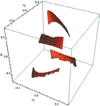
(c)   (d)

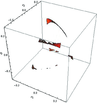
Figure 1: (Color online) Surfaces of constant OWID: (a) $s=0.3$, $\Delta^{\rightarrow}(\rho^{ab})=0.03$; (b) $s=0.5$, $\Delta^{\rightarrow}(\rho^{ab})=0.03$; (c) $s=0.3$, $\Delta^{\rightarrow}(\rho^{ab})=0.15$; (d) $s=0.5$, $\Delta^{\rightarrow}(\rho^{ab})=0.15$.

IV Dynamics of OWID under local nondissipative channels

In the following we consider that the state in Eqs.(63), (64) undergoes the phase flip channel Maziero , with the Kraus operators $\Gamma_{0}^{(A)}=$ diag$(\sqrt{1-p/2},\sqrt{1-p/2})\otimes I$, $\Gamma_{1}^{(A)}=$ diag$(\sqrt{p/2},-\sqrt{p/2})\otimes I$, $\Gamma_{0}^{(B)}=I\otimes$ diag$(\sqrt{1-p/2},\sqrt{1-p/2})$, $\Gamma_{1}^{(B)}=I\otimes$ diag$(\sqrt{p/2},-\sqrt{p/2})$, where $p=1-\exp(-\gamma t)$, $\gamma$ is the phase damping rate Maziero ; yu . Let $\varepsilon(\cdot)$ represent the operator of decoherence. Then under the phase flip channel we have

$$\varepsilon(\rho) = \frac{1}{4}(I\otimes I+I\otimes s\sigma_{3}+(1-p)^{2}c_{1}\sigma_{1}\otimes\sigma_{1}$$ (77)

$$+(1-p)^{2}c_{2}\sigma_{2}\otimes\sigma_{2}+c_{3}\sigma_{3}\otimes\sigma_{3}).$$

As $\varepsilon(\rho)$ satisfies conditions in Eqs.(63), (64), and the OWID of the $\rho^{ab}$ under the phase flip channel is given by

$$\Delta^{\rightarrow}(\varepsilon(\rho^{ab})) = \frac{1}{4}[(1-c_{3}+\sqrt{s^{2}+(1-p)^{4}(c_{1}+c_{2})^{2}})\log(1-c_{3}+\sqrt{s^{2}+(1-p)^{4}(c_{1}+c_{2})^{2}})$$ (78)

$$+(1-c_{3}-\sqrt{s^{2}+(1-p)^{4}(c_{1}+c_{2})^{2}})\log(1-c_{3}-\sqrt{s^{2}+(1-p)^{4}(c_{1}+c_{2})^{2}})$$

$$+(1+c_{3}+\sqrt{s^{2}+(1-p)^{4}(c_{1}+c_{2})^{2}})\log(1+c_{3}+\sqrt{s^{2}+(1-p)^{4}(c_{1}+c_{2})^{2}})$$

$$+(1+c_{3}-\sqrt{s^{2}+(1-p)^{4}(c_{1}+c_{2})^{2}})\log(1+c_{3}-\sqrt{s^{2}+(1-p)^{4}(c_{1}+c_{2})^{2}})]$$

$$-\frac{1}{4}[(1+s-c_{3})\log(1+s-c_{3})+(1+s+c_{3})\log(1+s+c_{3})$$

$$+(1-s-c_{3})\log(1-s-c_{3})+(1-s+c_{3})\log(1-s+c_{3})].$$

As an example, for $s=0.3,c_{1}=0.3,c_{2}=-0.4,c_{3}=0.56$, the dynamic behavior of correlation of the state under the phase flip channel is depicted in Fig.2. We find that the concurrence $C$ is greater than the OWID for $0\leq P\leq 0.237211$ and a sudden death of entanglement appears at $p=0.321904,$ here one sees that the concurrence become zero after the transition. Therefore for these states the entanglement is weaker against the decoherence than the OWID.

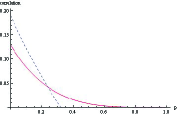
Figure 2: (Color online) Concurrence(blue dashed line) and OWID(red solid line) under phase flip channel for $s=0.3$, $c_{1}=0.3,$ $c_{2}=-0.4$ and $c_{3}=0.56$.

V summary

We have studied the OWID for a class of $X$ states. The level surfaces of the OWID have been depicted. For $r=s=0$ our results reduce to the ones for Bell-diagonal states. For nonzero $s$, it has been shown that the level surfaces of the OWID may have quite different geometry. The OWID become smaller in certain time interval for some initial states, and for some states the OWID is stronger against the decoherence than the entanglement.

Acknowledgments This work was supported by the NSFC 11101017, KZ201210028032 and PHR201007107.

References

- (1) C. H. Bennett and S. Wiesner, Phys. Rev. Lett. 69, 2881(1992).
- (2) C. H. Bennett, G. Brassard, Crépeau, R. Jozsa, A. Peres, and W. K. Wootters, Phys. Rev. Lett. 70, 1895 (1993).
- (3) A. K. Ekert, Phys. Rev. Lett. 67, 661 (1991).
- (4) A. K. Pati, Phys. Rev. A 63, 014302 (2000); C. H. Bennett, D. P. DiVincenzo, P. W. Shor, J. A. Smolin, B. M. Terhal, and W. K. Wootters, Phys. Rev. Lett. 87, 077902 (2001).
- (5) C. H. Bennett, D. P. DiVincenzo, C. A. Fuchs, T. Mor, E. Rains, P. W. Shor, J. A. Smolin and W. K. Wootters, Phys. Rev. A 59, 1070 (1999).
- (6) L. Henderson and V. Vedral, J. Phys. A 34, 6899 (2001); H. Ollivier and W. H. Zurek, Phys. Rev. Lett. 88, 017901(2002).
- (7) K. Modi, T. Paterek, W. Son, V. Vedral, and M. Williamson, Phys. Rev. Lett. 104, 080501 (2010).
- (8) R. Auccaise, J. Maziero, L. C. Céleri, D. O. Soares-Pinto, E. R. deAzevedo, T. J. Bonagamba, R. S. Sarthour, I. S. Oliveira, and R. M. Serra, Phys. Rev. Lett. 107, 070501 (2010).
- (9) G. L. Giorgi, B. Bellomo, F. Galve, and R. Zambrini, Phys. Rev. Lett. 107, 190501 (2011).
- (10) A. Streltsov, G. Adesso, M. Piani, and D. BruBruß, Phys. Rev. Lett. 109, 050503 (2012).
- (11) K. Modi, A. Brodutch, H. Cable, T. Paterek and V. Vedral, Rev. Mod. Phys. 84. 1655 (2012).
- (12) M. Ali, A. R. P. Rau, G. Alber, Phys. Rev. A 81, 042105 (2010).
- (13) B. Li, Z. X. Wang and S. M. Fei, Phys. Rev. A 83, 022321 (2011).
- (14) Q. Chen, C. Zhang, S. Yu, X. X. Yi and C. H. Oh, Phys. Rev. A 84, 042313 (2011).
- (15) M. Shi, C. Sun, F. Jiang, X. Yan and J. Du, Phys. Rev. A 85, 064104 (2012).
- (16) S. Vinjanampathy, A. R. P. Rau, J. Phys. A 45, 095303 (2012).
- (17) R. Horodecki and M. Horodecki, Phys. Rev. A 54, 1838 (1996).
- (18) M. D. Lang and C. M. Caves, Phys. Rev. Lett. 105, 150501 (2010).
- (19) Y. Yao, H. W. Li, Z. Q. Yin, and Z. F. Han, Physics Letters A 376, 358 (2012).
- (20) J. Oppenheim, M. Horodecki, P. Horodecki and R. Horodecki, Phys. Rev. Lett. 89, 180402 (2002).
- (21) M. Horodecki, K. Horodecki, P. Horodecki, R. Horodecki, J. Oppenheim, A. Sen(De) and U. Sen, Phys. Rev. Lett. 90, 100402 (2003).
- (22) S. Luo, Phys. Rev. A 77, 042303 (2008).
- (23) M. Piani, P. Horodecki and R. Horodecki, Phys. Rev. Lett. 100, 090502 (2008).
- (24) S. Wu, U. V. Poulsen and K. Mølmer, Phys. Rev. A 80, 032319 (2009).
- (25) K. Modi, T. Paterek, W. Son, V. Vedral and M. Williamson, Phys. Rev. Lett. 104, 080501 (2010).
- (26) S. Luo and S. Fu, Phys. Rev. A 82, 034302 (2010).
- (27) B. Dakic, V. Vedral, and C. Brukner, Phys. Rev. Lett. 105,190502 (2010).
- (28) G. Adesso and A. Datta, Phys. Rev. Lett. 105, 030501 (2010).
- (29) P. Giorda and M. G. A. Paris, Phys. Rev. Lett. 105, 020503 (2010).
- (30) W. H. Zurek, Phys. Rev. A 67, 012320 (2003).
- (31) M. Horodecki, P. Horodecki, R. Horodecki, J. Oppenheim, A. Sen(De), U. Sen and B. Synak, Phys. Rev. A 71, 062307 (2005); M. Horodecki, P. Horodecki and J. Oppenheim, Phys. Rev. A 67, 062104 (2003).
- (32) J. Oppenheim, K. Horodecki, M. Horodecki, P. Horodecki and R. Horodecki, Phys. Rev. A 68, 022307 (2003).
- (33) A. Streltsov, H. Kampermann and D. Bruß, Phys. Rev. Lett. 108, 250501 (2012).
- (34) T. K. Chuan, J. Maillard, K. Modi, T. Paterek, M. Paternostro and M. Piani, Phys. Rev. Lett. 109, 070501 (2012).
- (35) A. Streltsov, H. Kampermann and D. Bruß, Phys. Rev. Lett. 106, 160401 (2011).
- (36) H. Kim, M. R. Hwang, E. Jung and D. Park, Phys. Rev. A 81, 052325 (2010).
- (37) M. A. Nielsen and I. L. Chuang, Quantum Computation and Quantum Information (Cambridge University Press, Cambridge, UK, 2000).
- (38) J. Maziero, L. C. Céleri, R. M. Serra and V. Vedral, Phys. Rev. A 80, 044102 (2009).
- (39) T. Yu and J. H. Eberly, Phys. Rev. Lett. 97, 140403 (2006).