Astrometric Reverberation Mapping

Abstract

Spatially extended emission regions of Active Galactic Nuclei (AGN) respond to continuum variations, if such emission regions are powered by energy reprocessing of the continuum. The response from different parts of the reverberating region arrives at different times lagging behind the continuum variation. The lags can be used to map the geometry and kinematics of the emission region (i.e., reverberation mapping, RM). If the extended emission region is not spherically symmetric in configuration and velocity space, reverberation may produce astrometric offsets in the emission region photocenter as a function of time delay and velocity, detectable with future $\mu$as to tens of $\mu$as astrometry. Such astrometric responses provide independent constraints on the geometric and kinematic structure of the extended emission region, complementary to traditional reverberation mapping. In addition, astrometric RM is more sensitive to infer the inclination of a flattened geometry and the rotation angle of the extended emission region.

1. Introduction

Reverberation mapping (RM) is a powerful tool to probe the structure of the broad emission line region (BLR) in AGNs and quasars (e.g., Blandford & McKee, 1982; Peterson, 1993) without the need to resolve the BLR. The basic ideas are that the BLR is powered by photoionization by the (ionizing) continuum from the accreting black hole and that it responds to the variations of the continuum in a light crossing time. The response from different parts of the BLR will arrive at different time delays with respect to the continuum variation. Thus by mapping a two-dimensional broad line response function in the time delay and velocity plane (velocity-delay maps, e.g., Blandford & McKee, 1982; Horne et al., 2004) one can in principle recover the geometry and kinematics of the BLR. Over the past several decades, RM has proven to be a practical technique in studying the structure of BLRs. Although accurate velocity-time delay mapping is still lacking, RM studies have successfully measured average BLR sizes for several dozens of AGNs and quasars (e.g., Kaspi et al., 2000, 2007; Peterson et al., 2004; Bentz et al., 2009a, b), and in a few cases, crude velocity-delay maps (e.g., Denney et al., 2009; Bentz et al., 2010).

RM studies have shown that the typical BLR size $R$ scales approximately with the AGN luminosity $L^{0.5}$. In the latest version of the $R-L$ relation (e.g., Bentz et al., 2009a), $\log(R/{\rm light\,days})=-21.3+0.519\log(\lambda L_{\lambda}(5100\textrm{\AA})/{\rm erg\,s^{-1}})$. Thus for typical quasar luminosities ($\lambda L_{\lambda}(5100\textrm{\AA})=10^{45}\,{\rm erg\,s^{-1}}$, or bolometric luminosity $L_{\rm bol}\approx 10^{46}\,{\rm erg\,s^{-1}}$) at $z\sim 0.5$, the BLR size is $\sim 0.1\,{\rm pc}$ ($\sim 15\,\mu$as). This scale is 3 orders of magnitude smaller than the diffraction limit of 10m class optical telescopes (${\cal\theta}\sim$ tens of mas). Optical/near-IR interferometry with $\mu$as resolution has yet to come. Thus reverberation mapping will remain one of the few practical methods to measure the BLR size, along with microlensing in gravitationally lensed quasars (e.g., Morgan et al., 2010; Sluse et al., 2011).

However, measuring the source photocenter positions can achieve a factor of $\sim 1/\sqrt{N_{\rm photon}}$ enhancement in precision compared with the image resolution (e.g., Lindegren, 1978; Bailey, 1998a), where $N_{\rm photon}$ is the number of photons received in a bandpass. This means for $10^{6}$ photons, the achievable astrometry precision is 3 orders of magnitude smaller than the image resolution. One application of this idea is spectroastrometry (e.g., Bailey, 1998a), where differential astrometric positions as a function of wavelength (velocity) can be used to probe otherwise unresolved sources (e.g., Bailey, 1998b; Gnerucci et al., 2011).

When the astrometric precision approaches the angular BLR size, it becomes possible to study the BLR structure with astrometric signatures. A simple application would be to use spectroastrometry to place constraints on the BLR structure. A more radical possibility, however, is to detect and model the wobble in the broad line emission photocenter due to reverberation to the continuum variations, since the different arrival times of the BLR response will cause shifts in the observed BLR photocenter.

In this work we investigate the feasibility of combing the traditional intensity RM with astrometric information. Unlike spectroastrometry, the reverberation of the BLR will directly induce shifts in the photocenter position of broad line emission as a function of time delay and velocity. As we will show below, the pattern of photocenter shifts is determined by the geometry and kinematics of the BLR, thus providing independent constraints on the BLR structure, complementary to traditional intensity RM. Although our main focus is on the BLR, this method can be readily applied to the reverberation of the dust torus of AGNs (e.g., Suganuma et al., 2006) or other reverberation systems, where the required astrometric precision might be less stringent. We describe the basic formalism in §2 and demonstrate this method in §3 and §4 with simple models for the BLR. We briefly discuss the practical issues with this method in §5, with an overview on the perspectives of achieving the required astrometric precision in the near future in §5.2, and conclude in §6.

2. Basic Formalism

Let us set up a 3-dimensional cartesian coordinate system (in the observer frame) centered on the continuum source (e.g., the inner edge of the accretion disk, which we treat as a point source), and let the observer be at $z=+\infty$. The time delay of response from each point $\mathbf{r}\equiv(x,y,z)$ in the BLR is then simply:

$$\tau(\mathbf{r})=r-z=\sqrt{x^{2}+y^{2}+z^{2}}-z=r(1-\cos\theta)\ ,$$ (1)

where we use units that normalize the speed of light to $c=1$, $r$ is the distance to the central source, and $\theta$ is the angle between vector $\mathbf{r}$ and $+z$ axis. Obviously the iso-delay surface (i.e., the surface with constant time delay) is a paraboloid for an observer located at infinity. Points on the $+z$ axis, i.e., on the near side along the line-of-sight (hereafter los), have zero time delay with respect to the continuum variations.

Assuming that the observed continuum increases at time $t=0$ by a constant amount $f_{c}$ for a certain amount of time $\Delta t$, and goes back to normal at $t=\Delta t$, i.e., the change in continuum luminosity is

$$\delta_{c}(t) = \left\{\begin{array}[]{ll}0,&t<0\\ f_{c},&0<t<\Delta t\\ 0,&t>\Delta t\ .\end{array}\right.$$ (5)

The response in the broad line intensity is then a function of time $t$ and los velocity $v$

$$\delta_{\rm em}(t,v)=\int j(\mathbf{r})g(v,\mathbf{r},\mathbf{w})\delta_{c}\left(t-\tau(\mathbf{r})\right)d\mathbf{r}d\mathbf{w}\ ,$$ (6)

where $j(\mathbf{r})$ is the (assumed isotropic) responding volume emissivity of the emission region as a function of position, and

$$g(v,\mathbf{r},\mathbf{w})=f(\mathbf{r},\mathbf{w})\delta(v-\mathbf{w}\cdot\mathbf{n})\$$ (7)

where $(\mathbf{r,w})$ are the 3D coordinate and velocity vectors, $f(\mathbf{r},\mathbf{w})$ is the normalized (e.g., $\int fd\mathbf{w}=1$) 3D velocity distribution at point $\mathbf{r}$, determined by the kinematic structure of the BLR, and $\mathbf{n}\equiv+\hat{z}$ denotes the unit vector of the los. Note that Eqn. (6) is equivalent to the traditional RM equation invoking the transfer function (i.e., the line intensity response for a $\delta$-function continuum flare; Blandford & McKee, 1982; Peterson, 1993). However, for simplicity we shall avoid the usage of transfer function and work directly in the time domain in terms of the observed line intensity and photocenter positon for different velocity channels (see, e.g., Pancoast et al., 2011).

If we further assume that the BLR is transparent to its own emission, i.e., neglecting absorption and scattering (as generally assumed in RM), then the projected photocenter position of the responding emission with los velocity $v$ as observed by the distance observer is

$$x_{0}(t,v) = \displaystyle\frac{\int xj(\mathbf{r})g(v,\mathbf{r},\mathbf{w})\delta_{c}\left(t-\tau(\mathbf{r})\right)d\mathbf{r}d\mathbf{w}}{\int j(\mathbf{r})g(v,\mathbf{r},\mathbf{w})\delta_{c}\left(t-\tau(\mathbf{r})\right)d\mathbf{r}d\mathbf{w}}$$

$$y_{0}(t,v) = \displaystyle\frac{\int yj(\mathbf{r})g(v,\mathbf{r},\mathbf{w})\delta_{c}\left(t-\tau(\mathbf{r})\right)d\mathbf{r}d\mathbf{w}}{\int j(\mathbf{r})g(v,\mathbf{r},\mathbf{w})\delta_{c}\left(t-\tau(\mathbf{r})\right)d\mathbf{r}d\mathbf{w}}\ .$$ (8)

The projected photocenter position integrated over all los velocities is:

$$x_{0}(t)=\displaystyle\frac{\int xj(\mathbf{r})\delta_{c}\left(t-\tau(\mathbf{r})\right)d\mathbf{r}}{\int j(\mathbf{r})\delta_{c}\left(t-\tau(\mathbf{r})\right)d\mathbf{r}}\ ,y_{0}(t)=\displaystyle\frac{\int yj(\mathbf{r})\delta_{c}\left(t-\tau(\mathbf{r})\right)d\mathbf{r}}{\int j(\mathbf{r})\delta_{c}\left(t-\tau(\mathbf{r})\right)d\mathbf{r}}\ .$$

In Eqn. (5), if $c\Delta t$ is much smaller compared with the typical BLR size $R$, then the continuum light curve can be treated as a (square wave) $\delta-$function. In this case the near side of the BLR completes reverberation (i.e., back to the steady level) before the far side reverberation reaches the observer. On the other hand, if $c\Delta t\gg R$, then the continuum light curve is a step function, and the near side of the BLR will still be in the high state when the far side reverberation reaches the observer. In the following discussion, we will consider the two limiting cases where $c\Delta t\ll R$ (a continuum flare) and $c\Delta t\gg R$ (a continuum jump).

3. Simple Geometric and Kinematic Models for the BLR

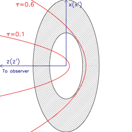
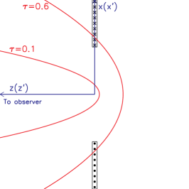
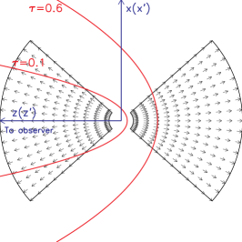
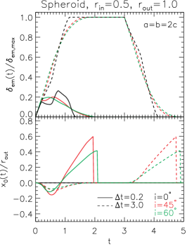
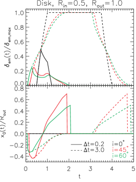
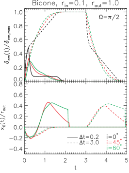
Figure 1.— Illustrative examples of BLR geometry and kinematics for the three non-spherical models described in §3, and for the velocity-integrated reverberation amplitude $\delta_{\rm em}(t)$ and photocenter position $x_{0}(t)$. The top panels show the cross section (regions filled with different patterns) in the $xz$ plane for three BLR geometries when the BLR intrinsic coordinate system $x^{\prime}y^{\prime}z^{\prime}$ is aligned with the observer coordinate system $xyz$. The red curves are typical parabolic iso-delay curves with constant $\tau$ (in the same units as in Eqn. 1). The bottom panels show the corresponding reverberation mapping signals. Left: an oblate spheroid model with $a=b=2c=1$, $r_{\rm in}=0.5$ and $r_{\rm out}=1$. Middle: a truncated disk model with $R_{\rm in}=0.5$ and $R_{\rm out}=1$. Right: a biconical outflow with $r_{\rm in}=0.1$, $r_{\rm out}=1.0$, and an opening solid angle $\Omega=\pi/2$. In all examples, the intrinsic coordinates of the BLR ($x^{\prime}y^{\prime}z^{\prime}$) are rotated about the $y$-axis in the observer frame by an inclination angle $i$, such that the projected BLR in the $xy$ plane has planar symmetry about the $x$-axis (hence $y_{0}(t)\equiv 0$). For each model we compute for three inclination angles $i=0^{\circ},45^{\circ},60^{\circ}$, and two continuum variation timescales $\Delta t=0.2$ and $0.3$. In the $i=0^{\circ}$ cases, there is no photocenter offset as a function of time due to symmetry. We define the maximum-possible reverberation intensity as the one where the entire BLR is reverberating.

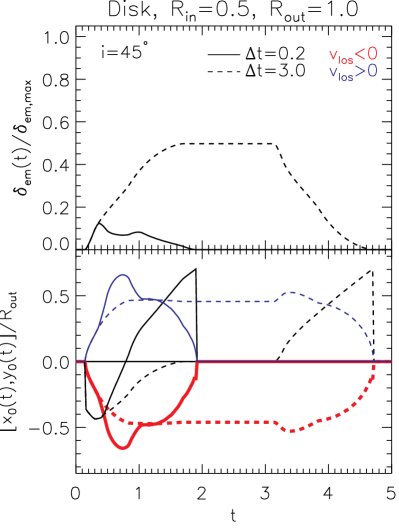
Figure 2.— Velocity-resolved evolution of reverberation intensity and photocenter positions, for the same disk model as in Fig. 1 with a los angle $i=45^{\circ}$ and two continuum variation timescales $\Delta t=0.2,3$. Due to symmetry, the intensity $\delta_{\rm em}$ and $x$-positions of the photocenter have identical time evolution for the blueshifted and redshifted halves of the disk, which are denoted by the black lines. On the other hand, the $y$ photocenter positions have time evolutions denoted by the blue and (thicker) red lines for the blueshifted and redshifted halves, which are symmetric about the $x$-axis.

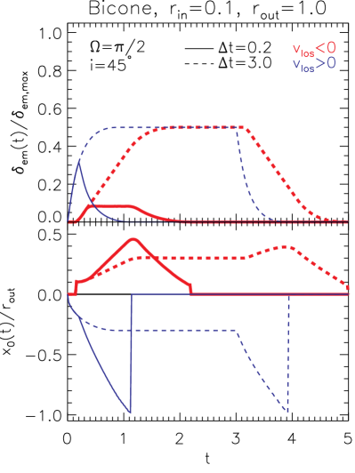
Figure 3.— Velocity-resolved evolution of reverberation intensity and photocenter position $x_{0}(t)$, for the same bicone model as in Fig. 1 with a los angle $i=45^{\circ}$ and two continuum variation timescales $\Delta t=0.2,3$. The blueshifted cone (denoted by blue lines) and the redshifted cone (denoted by thicker red lines) have quite different time evolution in reverberation intensity $\delta_{\rm em}$ and photocenter position $x_{0}(t)$, reflecting the geometry and kinematics of the bicone BLR structure. The photocenter position $y_{0}(t)\equiv 0$ due to symmetry in the projected $xy$ plane.

To demonstrate the astrometric signals from RM, we use simple geometric and kinematic models for the BLR, and study the reverberation process. But our approach below is applicable to general cases.

There are few observational constraints on the structure of the BLR. Spherical BLRs will not produce any photocenter offset. However, there is evidence that the BLR motion may be dominated by rotation, and the BLR may have a flattened geometry. Such evidence comes from the dependence of broad line width on orientation angle inferred from radio properties (e.g., Wills & Browne, 1986; Jarvis & McLure, 2006), or from modeling the broad line profiles (e.g., Kollatschny & Zetzl, 2011). In the extreme case, the broad lines in $\lesssim 10\%$ AGNs show a characteristic double-peaked profile, commonly interpreted as arising from a disk geometry with Keplerian rotation (e.g., Eracleous & Halpern, 1994). On the other hand, radial motion of the BLR has been inferred from velocity-resolved reverberation mapping in several AGNs (e.g. Denney et al., 2009), and it has been suggested that the high-ionization broad line (such as CIV) may have a component originating from a disk wind (e.g., Murray et al., 1995; Proga et al., 2000). It is possible that virial motion and radial motion coexist in the BLR.

Motivated by these observations, we consider the following simple classes of geometry and kinematics for the BLR. In all cases we assume constant density of the BLR, and we assume uniform reprocessing coefficient $\epsilon$ across the entire BLR. Therefore the volume emissivity $j(\mathbf{r})\equiv\epsilon L_{c}/(4\pi r^{2})$ is proportional to $1/r^{2}$, i.e., spherical shells with the same thickness but different radii will have the same total reverberation intensity. Again, we emphasize that our approach is not limited to these assumptions. We establish an intrinsic coordinate system $(x^{\prime}y^{\prime}z^{\prime})$ anchored to the BLR, which is rotated from the observer coordinate system $(x,y,z)$ by Euler angles $(\alpha,\beta,\gamma)$.

1. A triaxial ellipsoid configuration distributed within a shell: $r_{\rm in}^{2}<\displaystyle\frac{x^{\prime 2}}{a^{2}}+\frac{y^{\prime 2}}{b^{2}}+\frac{z^{\prime 2}}{c^{2}}<r_{\rm out}^{2}$. We further consider a sub-class of this configuration, an oblate spheroid where $a=b>c$, which probably more represents a flattened BLR geometry. The velocity field is assumed to be Maxwellian, with 1D dispersion equal to the virial velocity at each radius. Spherical shell geometries are also simplified versions of this model.

2. A truncated circular razor-thin disk ($R_{\rm in}<R<R_{\rm out}$) in the $x^{\prime}y^{\prime}$ plane, with an inclination angle $i$ from the los ($z$-axis in the observer frame). We assume a Keplerian velocity field for the disk and the disk rotation is counter-clockwise viewed from $z^{\prime}=+\infty$.

3. A biconical configuration, which is rotationally symmetric about the $z^{\prime}$-axis with an opening solid angle $\Omega$, and a radial extent from $r_{\rm in}$ to $r_{\rm out}$. The bicone has an inclination angle $i$ from the los ($z$-axis in the observer frame). We assume a biconical radial outflowing velocity structure. The detailed outflow velocity structure is not important in this work, as we will only consider the blueshifted and redshifted halves of the broad line profile.

To study reverberation mapping in emission line intensity and photocenter offsets for arbitrary geometry and kinematics, we discretize the emission region with a fine cartesian grid of cells $(x_{i},y_{i},z_{i})$ and assign velocities to each cell. At each time $t$, we determine the cells that are reverberating, i.e., $\delta_{c}(t-\tau(x_{i},y_{i},z_{i}))\neq 0$, and compute the reverberation quantities $\delta_{\rm em}$, $x_{0}$ and $y_{0}$ in Eqns. (6) and (2) with direct summation. This discrete method can efficiently handle any geometry and kinematics to sufficient numeric accuracy compared with integrating Eqns. (6) and (2). For simplicity we adopt the units $c=G=M=1$, where $G$ is the gravitational constant and $M$ is the central black hole mass.

4. Results

In the simplest case of a thin spherical shell (with radius $R$) model for the emission line region, the time evolution of the reverberation intensity has simple analytical forms (e.g., Bahcall et al., 1972), which we verified with our numerical approach. However, due to the spherical geometry, the photocenter does not show any offset as a function of time.

Fig. 1 shows several examples for the three non-spherical models described in §3, for the velocity-integrated case. Since all three models have rotational symmetry, we need only focus on the photocenter offset in the $x$-direction, i.e., the rotation of our model BLR preserves symmetry about the $x$-axis in the projected $xy$ plane. Specifically, the intrinsic coordinate system of the BLR $(x^{\prime}y^{\prime}z^{\prime})$ is rotated about the $y$-axis in the observer frame by inclination angle $i$.

For each model we compute for three orientations $i=0,45^{\circ},60^{\circ}$ and two continuum variability durations $\Delta t=0.2$ and $3$. In all cases the maximum BLR radius is set to be 1. It is clear from Fig. 1 that similar information is encoded in the photocenter reverberation maps as in the traditional intensity reverberation map. However, the photocenter reverberation maps are more sensitive to the inclination of the flattened BLR geometry than the intensity reverberation maps. The maximum photocenter offset is on the same order as the flux-weighted average size of the BLR. We will return to these points in §5.

In the examples shown in Fig. 1, a generic feature of the photocenter reverberation is the transition from the near-side photocenter to the far-side photocenter. If the duration of the continuum variation $\Delta t$ is short compared with the BLR size (e.g., a flash), this transition is continuous. On the other hand, if the duration $\Delta t$ is long, then there will be a period with no photocenter offset (i.e., the entire BLR is lit up). The spheroid geometry and the disk geometry result in similar astrometric RM signatures. This is expected because the spheroid model used is close to a flattened disk geometry. In both cases we see a gradual rise followed by a sharp cutoff around the maximum photocenter offset after the continuum returns to the base value. However, in the bicone geometry, the sharp cutoff occurs later past the peak photocenter offset. This difference is caused by the different edge geometry in these models – in the disk and spheroid cases, fewer and fewer materials are located at the far side of the emission region, which is opposite in the bicone case.

Another point worth noting is that for inclined BLRs, the total line intensity reverberation $\delta_{\rm em}(t)$ looks similar in different models, thus does not offer much differentiating power (e.g., Horne et al., 2004). However, the different behaviors in photocenter reverberation $x_{0}(t)$ for the flattened geometry and for the bicone geometry might be useful in distinguishing the two geometries.

The astrometric reverberation mapping signals vanish when the iso-delay surface is axisymmetric about the $z$-axis. For instance, an edge-on disk will not produce photocenter offset as a function of time delay for the velocity-integrated broad line flux. Fortunately, an astrometric signal will still arise if we have velocity-resolved reverberation mapping: the blue side of the reverberating broad line has a photocenter shifted from that of the red side. Thus the astrometric feature can determine the angular momentum direction of the disk-like BLR, while the traditional intensity reverberation mapping is unable to derive such information.

Similarly, velocity-resolved reverberation mapping in flux amplitude and in photocenter offset is a powerful tool to further constrain the velocity field of the BLR. Below we use the three models to demonstrate the different reverberation behaviors in the blueshifted and redshifted halves of the line profile.

1. Spheroid models. Since we assumed a random Maxwellian velocity distribution, the red part and blue part of the emission line profile have identical behavior in reverberation signals.

2. Disk models. We consider the disk example of $i=45^{\circ}$ shown in Fig. 1. In this case the redshifted part ($v_{\rm los}<0$) and blueshifted part ($v_{\rm los}>0$) of the disk will behave exactly the same in terms of $\delta_{\rm em}(t)$ and $x_{0}(t)$, except that the amplitude of $\delta_{\rm em}(t)$ is reduced by half. However, since we are now looking at half of the disk, the $y$ photocenter position of the redshifted/blueshifted disk changes as a function of time, as indicated by the red/blue lines in Fig. 2.

3. Bicone outflow models. We consider the bicone example of $i=45^{\circ}$ and $\Omega=\pi/2$ shown in Fig. 1. In this example the near-side cone has blueshifted velocity while the far-side cone has redshifted velocity. We plot the results for both cones in Fig. 3. The line intensity $\delta_{\rm em}$ is already different for the blueshifted half and redshifted half, since the two cones have distinct los velocities: we see intensity reverberation from the blueshifted cone (near-side) earlier than the redshifted cone (far-side). The time evolution of the $x$ photocenter position is also different for the blueshifted and redshifted cones. The $y$ photocenter positions for the two cones are always zero due to the symmetry of this example.

In the traditional case, velocity-resolved intensity RM can effectively distinguish outflow/inflow kinematics from virial motion (either in a Keplerian disk or in randomly orientated orbits) of the emission line region. The distinction between the two kinds of kinematics is also clearly reflected in the velocity-resolved astrometric RM, i.e., the time evolution of the blueshifted and redshifted photocenters is asymmetric in the outflow/inflow case, and symmetric in the case of virial motion (cf. Figs. 2 and 3)

5. Discussion

5.1. Practical Concerns with this Method

The representative examples shown in §4 indicate that the expected astrometric signals are on the order of the BLR size. Then for typical quasar luminosities of $L_{\rm bol}\gtrsim 10^{46}\,{\rm erg\,s^{-1}}$, we expect such astrometric signals to be on the order of tens of $\mu$as at $z\sim 0.5$. For more luminous objects and/or at lower redshifts, the expected astrometric signals will be larger. For example, the quasar 3C 273 ($z=0.158,\lambda L_{\lambda}(5100\textrm{\AA})=8.6\times 10^{45}\,{\rm erg\,s^{-1}},V\sim 12.8$) has a measured H$\beta$ BLR size of $\sim 300\,$light days (Bentz et al., 2009a), corresponding to $\sim 90\,\mu$as at its redshift. If we further consider reverberation of the dust torus, then the expected astrometric signals would be even larger, e.g., $\gtrsim 100\,\mu$as for quasar luminosities. The sizes of the BLR and torus approximately scale with $L^{0.5}$, thus for Seyfert luminosities, $\mu$as astrometric precision might be necessary for astrometric RM.

However, even if the astrometry requirement is fulfilled (see §5.2), there are still several practical issues to consider. These will affect the target selection and observing strategy for a successful monitoring program. Detailed characterization of the adverse effects and methods to mitigate them are beyond the scope of this paper, and we only give a brief discussion here as a general guideline for future work.

First, the monitoring should be carried out in optical/near-IR to observe the restframe UV to near-IR broad emission lines (e.g., CIV, Mg ii, Balmer and Paschen lines) and adjacent continua. Tunable narrow-band filters are desired for the broad line imaging and reliable continuum subtraction. High photometric accuracy is generally required, and to detect and model the astrometric signals we need good cadence of monitoring data. The monitoring time baseline could span weeks to years, depending on the target. Observations of repeated reverberation events can be combined to provide improved model constraints, as long as the monitoring time span is much shorter than the dynamical timescale ($\tau_{\rm dyn}\sim R/V_{\rm FWHM}$) of the BLR.

Measuring the photocenter of the reverberating part of the BLR to the nominal astrometric accuracy poses a more difficult challenge. It requires the subtraction of the continuum and the steady-state BLR emission and subsequent measurement of the photocenter of the variable BLR emission without degrading the astrometric accuracy much. The use of narrow-band filters helps with this procedure, but also increases the integration time to achieve the required photometric precision. Take the broad H$\beta$ line for example, the typical restframe equivalent width is $\sim 70\,$Å (e.g., Shen et al., 2011). Thus for a $\sim 100\,$Å narrow-band filter centered on the redshifted H$\beta$ line at $z\sim 0.5$, the enclosed H$\beta$ line flux is $\sim 50\%$ of the total flux. The host galaxy contribution in this bandpass is negligible for quasar luminosities $\lambda L_{\lambda}(5100\textrm{\AA})>10^{45}\,{\rm erg\,s^{-1}}$, and reaches $\sim 20\%$ of the total continuum at $\lambda L_{\lambda}(5100\textrm{\AA})=10^{44.5}\,{\rm erg\,s^{-1}}$ (e.g., Shen et al., 2011). With SNR$>100$ for the PSF core, $>10\%$ fractional changes in the broad line flux can be detected. However, the centering accuracy of the variable BLR emission degrades as $\sigma_{\rm meas,var}\sim\sigma_{\rm meas}/f_{\rm var}$, where $\sigma_{\rm meas}$ is the nominal centering accuracy for the target and $f_{\rm var}$ is the fraction of the variable flux (from the reverberating BLR) to the total flux. Thus larger amplitudes in the continuum variations (hence larger reverberation amplitude) are always favored over smaller amplitudes, just as for traditional intensity RM. Optimal image subtraction methods may be required to isolate the variable BLR emission within the bandpass (e.g., Alard, 2000).

Finally, the real situation may deviate from the idealized case assumed in reverberation mapping, which will inevitably lead to complications. With better and better RM data sets, however, it is possible to incorporate additional physical ingredients, such as photoionization processes, absorption and scattering, more complex geometry/kinematics, etc., in the framework of combined intensity and astrometric RM.

5.2. Precision Astrometry in the Optical/Near-IR

We now discuss realistic timescales for achieving the astrometric precision ($\mu$as to tens of $\mu$as) required to detect the astrometric reverberation mapping signals. Such single-epoch astrometric precision is already under serious considerations for ground-based and space-based facilities.

5.2.1 ground-based facilities

The recent development of AO-assisted, high-angular resolution, near-infrared observations with large, single-aperture telescopes has dramatically improved the astrometry precision. Single-measurement precision of $\sim 200-300\,\mu$as has been routinely achieved on $8-10$m class telescopes (e.g., Lazorenko et al., 2009; Fritz et al., 2010). $\lesssim 100\,\mu$as single-epoch precision (stable over 2 months) has been demonstrated for the Palomar 200 inch Hale telescope in 2-minute exposures (Cameron et al., 2009), for stars with $K_{s}\lesssim 13$. At this level of precision, there are several important instrumental, atmospheric and astrophysical effects that need to be taken into account; and in most cases, optimized procedures or algorithms must be undertaken to minimize these effects (e.g., Cameron et al., 2009; Fritz et al., 2010; Trippe et al., 2010).

In the study by Cameron et al. (2009), it was shown that the dominant systematic error is due to atmospheric differential tilt jitter. This is the stochastic and achromatic fluctuation in the relative displacement of the target and the reference star due to the different columns of atmospheric turbulence traversed by the light from the two objects. Cameron et al. (2009) demonstrated that the tilt jitter effect can be largely mitigated by an optimal weighting scheme that uses a grid of reference stars to measure the pair-wise distances from the target. This optimal estimation technique can essentially reduce the error due to tilt jitter, $\sigma_{\rm TJ}$, below the centering accuracy $\sigma_{\rm meas}$, which is mostly determined by aperture size, photon noise, and properties of the PSF. Cameron et al. (2009) also provided an empirical formula to predict the astrometric performance of a single-conjugate AO system:

$$\sigma_{\rm tot}^{2}= \sigma_{\rm meas}^{2}+\sigma_{\rm TJ}^{2}=\left(\frac{1.4\,{\rm sec}}{t}\right)\bigg{\{}\left[2\,{\rm mas}\left(\frac{2}{N}\right)^{0.3}\left(\frac{5\,{\rm m}}{D}\right)^{2}\right]^{2}$$ (10)

$$+\left[2\,{\rm mas}\left(\frac{2}{N}\right)^{0.7}\left(\frac{5\,{\rm m}}{D}\right)^{7/6}\right]^{2}\bigg{\}}\ ,$$

where $t$ is the integration time, $D$ is the telescope aperture diameter and $N$ is the number of reference stars. This formula suggests that for 20-minute exposures, the single-measurement precision can achieve $\sim 20\,\mu$as for $10$m-class telescopes, and $<10\,\mu$as for $30$m-class telescopes, with only a few reference stars in a $25$″$\times$$25$″ FOV. Note that with these large-aperture telescopes and a reasonable amount of exposure time (e.g., 30-60 min), the magnitude limit achievable with the above astrometric precision can be as faint as $K_{s}\sim 18$ by extrapolation (e.g., Cameron et al., 2009; Trippe et al., 2010), relevant for reverberation monitoring of AGN continuum and broad line fluxes.

The above estimation might be optimistic. The actual astrometric performance will inevitably depend on the telescope and AO systems, as well as target properties. Trippe et al. (2010) performed a detailed study on the limiting factors on the astrometry precision for the Multi-adaptive optics Imaging CAmera for Deep Observations (MICADO) proposed for the 42-m European Extremely Large Telescope (E-ELT). The dominant error terms include: instrumental geometric distortion $\sigma_{\rm dist}\sim 30\,\mu$as, chromatic atmospheric differential refraction (CDR) $\sigma_{\rm CDR}\sim 20\,\mu$as, atmospheric differential tilt jitter $\sigma_{\rm TJ}\sim 10\,\mu$as (with few minutes of integration), anisoplanatism of the multi-conjugate AO system $\sigma_{\rm aniso}\sim 8\,\mu$as, using galaxies as astrometric references in high galactic-latitude fields $\sigma_{\rm galaxies}\sim 20\,\mu$as, and calibration of the projected pixel scale $\sigma_{\rm scale}\lesssim 10\,\mu$as. Combining these error terms, Trippe et al. (2010) estimated a total error budget of $\sigma_{\rm sys}\sim 40\,\mu$as. In practice, some of these error terms can be reduced. For instance, $\sigma_{\rm CDR}$ can be effectively suppressed if narrow-band filters are used or special algorithms and observing strategies are deployed to correct for the CDR (e.g., Cameron et al., 2009). Note that for BLR reverberation mapping, it is preferable to use narrow-band filters to cover the emission lines and nearby continuum. $\sigma_{\rm galaxies}$ can also be reduced for AGN/quasar fields where there are a suitable number of reference stars. It is also possible to correct instrumental distortion by dedicated calibration procedures to control $\sigma_{\rm dist}$ down to the level of $\sim 10-30\,\mu$as (e.g., Trippe et al., 2010). Thus the range of single-epoch astrometry precision for this particular instrument on E-ELT is $\sim 20-40\,\mu$as, although the lower bound would be very challenging to achieve. We expect similar performance for other 30m-class telescopes.

An alternative route to single-aperture precision astrometry is long-baseline astrometry that operates in the very-narrow-angle regime (angular separation $\lesssim 30$″), which uses interferometry in optical/near-IR to achieve high relative astrometric precision (e.g., Shao & Colavita, 1992). For instance, the Very Large Telescope Interferometer (VLTI) instrument is designed to deliver an astrometric precision at the $\sim 30-40\,\mu$as level (van Belle et al., 2008). In the short term, however, the astrometric precision is likely limited, by the accuracy in determining the interferometer baseline, to $\sim 20-30\,\mu$as (e.g., van Belle, 2009). Moreover, current implementation of optical to near-IR interferometry usually requires bright target magnitude $K\lesssim 13$ (e.g., van Belle et al., 2008), hence is not yet suitable for AGN monitoring except for the brightest objects (such as 3C 273).

To summarize, ground-based facilities are promising to deliver $\lesssim$ tens of $\mu$as single-epoch astrometry precision within a decade or two, and in the most optimal cases, $\sim 10\,\mu$as precision. Single-aperture astrometry with large telescopes and AO (currently operating in the near-IR, with potential extension to the optical) is probably better suited for AGN targets than long-baseline interferometry at this stage. This precision can be achieved for relatively short integration ($\lesssim 1\,$hr) and faint target limit $K_{s}\lesssim 18$ relevant for AGN reverberation mapping. But to achieve this goal, dedicated calibration algorithms and observing strategies, along with systematic control of the telescope and instrument system, will all be necessary. This level of astrometry precision is suitable for BLR reverberation mapping of nearby AGNs and bright quasars, and sufficient for AGN dust reverberation mapping.

5.2.2 space-based facilities

The Hubble Space Telescope (HST) is currently the only space-based facility that can perform astrometry at the $\lesssim 1\,$mas precision (e.g., Anderson & King, 2000; Benedict et al., 2003). The future James Webb Space Telescope (JWST) can in principle deliver a similar precision (e.g., Diaz-Miller, 2007). Thus both HST and JWST are less favorable for precision astrometry compared with ground-based facilities discussed above.

GAIA (Perryman et al., 2001) is a space-based astrometry mission scheduled to launch in 2013, which can deliver 150 (400) $\mu$as single-measurement astrometric precision for $V<16$ (18) targets. This precision is not adequate for astrometric reverberation mapping of the BLRs, and barely enough for AGN dust torus reverberation.

Perhaps the best facility for astrometric AGN reverberation mapping is a mission similar to the SIM/SIM Lite mission (Unwin et al., 2008), which is capable of achieving $\sim 10\,\mu$as single-measurement precision for $V<18$ targets with a space-based 6-m baseline optical interferometer. In fact probing the $\lesssim\,$pc spatial extent of AGN/quasar jets and BLRs is one of the science cases for this mission, using the same technique as spectroastrometry. Astrometric reverberation mapping would be an ideal application with similar facilities for pointed multi-visit observations, yet with much more constraining power on the BLR (and torus) geometry and kinematics than spectroastrometry. Although this mission was canceled for the current decade, the technology for such a mission is already in place (e.g., Shao, 2010). In light of the exciting science that will be enabled with $\mu$as astrometry (especially with the driving force for exoplanet science), it is reasonable to anticipate similar missions to be approved in the next decade.

6. Conclusions

In this paper we outlined a simple idea of astrometric reverberation mapping: observing the astrometric “wobble” of the BLR photocenter in reverberation events. We demonstrated its potential in constraining the geometry and kinematic structure of the BLR with simple BLR models.

The virtue of astrometric RM is that it provides an independent set of time series that can be combined with the intensity RM data to constrain the BLR model. In addition, it is more sensitive to the inclination of a disk-like geometry and inference of its angular momentum direction, than intensity RM alone. Although the BLR is still unresolved, the spatial information from precision astrometry for the reverberating parts of the BLR greatly facilitates using reverberation mapping to probe the BLR structure. Once we have a set of high quality continuum and broad line flux monitoring time series with precision photometry and astrometry, we can fit the data in the time domain using model intensity light curves and photocenter evolution. General Markov Chain Monte Carlo approaches with Bayesian inference (e.g., Pancoast et al., 2011; Brewer et al., 2011) can be applied to search the parameter space of different model families and to quantify model uncertainties.

While conceptually simple, this method is not yet ready for immediate applications. We discussed realistic timescales for achieving the required astrometric precision ($\mu$as to tens of $\mu$as), and concluded that ground-based large-aperture telescopes with AO offer the best hope to apply this method to luminous quasars and dust torus RM within a decade or two, and a space-based interferometer (a SIM/SIM-Lite like mission) with $\mu$as astrometric precision in the next decade or two may extend this method to the Seyfert regime.

References

- Alard (2000) Alard, C. 2000, A&AS, 144, 363
- Anderson & King (2000) Anderson, J., & King, I. R. 2000, PASP, 112, 1360
- Bahcall et al. (1972) Bahcall, J. N., Kozlovsky, B.-Z., & Salpeter, E. E. 1972, ApJ, 171, 467
- Bailey (1998a) Bailey, J. 1998a, SPIE, 3355, 932
- Bailey (1998b) Bailey, J. 1998b, MNRAS, 301, 161
- Benedict et al. (2003) Benedict, G. F., et al. 2003, AJ, 126, 2549
- Bentz et al. (2009a) Bentz, M. C., et al. 2009a, ApJ, 697, 160
- Bentz et al. (2009b) Bentz, M. C., et al. 2009b, ApJ, 705, 199
- Bentz et al. (2010) Bentz, M. C., et al. 2010, ApJ, 720, L46
- Blandford & McKee (1982) Blandford, R. D., & McKee, C. F. 1982, ApJ, 255, 419
- Brewer et al. (2011) Brewer, B. J. 2011, ApJ, 733, L33
- Cameron et al. (2009) Cameron, P. B., Britton, M. C., & Kulkarni, S. R. 2009, AJ, 137, 83
- Denney et al. (2009) Denney, K. D., et al. 2009, ApJ, 704, L80
- Diaz-Miller (2007) Diaz-Miller, R. I. 2007, in ASP Conf. Ser. 364, The Future of Photometric, Spectrophotometric, and Polarimetric Standardization, ed. C. Sterken (San Francisco: ASP), 81
- Eracleous & Halpern (1994) Eracleous, M., & Halpern, J. P. 1994, ApJS, 90, 1
- Fritz et al. (2010) Fritz, T., et al. 2010, MNRAS, 401, 1177
- Gnerucci et al. (2011) Gnerucci, A., Marconi, A., Capetti, A., Axon, D. J., Robinson, A., & Neumayer, N. 2011, A&A, 536, 86
- Horne et al. (2004) Horne, K., Peterson, B. M., Collier, S. J., & Netzer, H. 2004, PASP, 116, 465
- Jarvis & McLure (2006) Jarvis, M. J., & McLure, R. J. 2006, MNRAS, 369, 182
- Kaspi et al. (2007) Kaspi, S., Brandt, W. N., Maoz, D., Netzer, H., Schneider, D. P., & Shemmer, O. 2007, ApJ, 659, 997
- Kaspi et al. (2000) Kaspi, S., Smith, P. S., Netzer, H., Maoz, D., Jannuzi, B. T., & Giveon, U. 2000, ApJ, 533, 631
- Kollatschny & Zetzl (2011) Kollatschny, W., & Zetzl, M. 2011, Nature, 470, 366
- Lazorenko et al. (2009) Lazorenko, P. F., et al. 2009, A&A, 505, 903
- Li et al. (2009) Li, L.-X., Narayan, R., & McClintock, J. E. 2009, ApJ, 691, 847
- Lindegren (1978) Lindegren, L. 1978, in IAU Colloq. 48, Modern Astrometry, ed. F. V. Prochazka & R. H. Tucker (Dordrecht: Kluwer), 197
- Morgan et al. (2010) Morgan, C. W., Kochanek, C. S., Morgan, N. D., & Falco, E. E. 2010, ApJ, 712, 1129
- Murray et al. (1995) Murray, N., Chiang, J., Grossman, S. A., & Voit, G. M. 1995, ApJ, 451, 498
- Pancoast et al. (2011) Pancoast, A., Brewer, B. J., & Treu, T. 2011, ApJ, 730, 139
- Peterson (1993) Peterson, B. M. 1993, PASP, 105, 247
- Peterson et al. (2004) Peterson, B. M., et al. 2004, ApJ, 613, 682
- Perryman et al. (2001) Perryman, M. A. C., et al. 2001, A&A, 369, 339
- Proga et al. (2000) Proga, D., Stone, J. M., & Kallman, T. R. 2000, ApJ, 543, 686
- Shao (2010) Shao, M. 2010, in ASP Conf. Ser. 430, Pathways Towards Habitable Planets, ed. V. C. du Foresto, D. M. Gelino, and I. Ribas (San Francisco: ASP), 213
- Shao & Colavita (1992) Shao, M., & Colavita, M. M. 1992, A&A, 262, 353
- Shen et al. (2011) Shen, Y., et al. 2011, ApJS, 194, 45
- Sluse et al. (2011) Sluse, D., et al. 2011, A&A, 528, 100
- Suganuma et al. (2006) Suganuma, M., et al. 2006, ApJ, 639, 46
- Trippe et al. (2010) Trippe, S., et al. 2010, MNRAS, 402, 1126
- Unwin et al. (2008) Unwin, S. C., et al. 2008, PASP, 120, 38
- van Belle et al. (2008) van Belle, G. T., et al. 2008, Msngr, 134, 6
- van Belle (2009) van Belle, G. T. 2009, NewAR, 53, 336
- Wills & Browne (1986) Wills, B. J., & Browne, I. W. A. 1986, ApJ, 302, 56