Scattering by linear defects in graphene: a continuum approach
Abstract
We study the low-energy electronic transport across periodic extended defects in graphene. In the continuum low-energy limit, such defects act as infinitesimally thin stripes separating two regions where Dirac Hamiltonian governs the low-energy phenomena. The behavior of these systems is defined by the boundary condition imposed by the defect on the massless Dirac fermions. We demonstrate how this low-energy boundary condition can be computed from the tight-binding model of the defect line. For simplicity we consider defect lines oriented along the zigzag direction, which requires the consideration of only one copy of Dirac equation. Three defect lines of this kind are studied and shown to be mappable between them: the pentagon-only, the and the defect lines. In addition, in this same limit, we calculate the conductance across such defect lines with size , and find it to be proportional to at low temperatures.
pacs:
81.05.ue, 72.80.Vp, 78.67.WjI Introduction
Graphene growth by chemical vapor deposition (CVD) on metal surfacesLi et al. (2009); Reina et al. (2009); Kim et al. (2009); Bae et al. (2010) is a very promising scalable method for producing graphene sheets. However, the present status of the method, typically results in the synthesis of polycrystalline graphene abundant in topological defects, grain boundaries (GBs) being, by far, the most common ones.Huang et al. (2011); Kim et al. (2011); Nemes-Incze et al. (2011)
Due to graphene’s hexagonal structure, pairs of pentagons and heptagons, named Stone-Wales (SW) defects, as well as octagons, are expected to form at graphene GBs.Stone and Wales (1986) Recent atomic resolution TEM studies Meyer et al. (2008); Lahiri et al. (2010); Huang et al. (2011); Kim et al. (2011) allowed the observation of GBs in CVD-grown graphene. These experimental studies have shown that the GBs are generally not perfect straight lines, and that the - defects along the boundaries are not periodic. Furthermore, as shown by recent TEM studies,Huang et al. (2011); Kim et al. (2011) these extended pentagon-heptagon defect-lines intercept each other at random angles, forming irregular polygons with edges showing a stochastic distribution of lengths. This renders theoretical studies of such defects difficult, in particular when using microscopic tight-binding models.Ferreira et al. (2011)
Theoretical studies have argued that GBs strongly influence the properties of graphene, namely its chemical,Malola et al. (2010) mechanical Yazyev and Louie (2010a); Grantab et al. (2011) and electronic ones. Electronic mobilities of films produced through CVD are lower than those reported on exfoliated graphene, because Novoselov et al. (2004, 2005) electronic transportCastro Neto et al. (2009); Peres (2010) is hindered by grains and GBs.Yazyev and Louie (2010b); Ferreira et al. (2011)
Recently, the observation of a linear extended defect acting as a one-dimensional conducting charged wireLahiri et al. (2010) stimulated some theoretical studies concentrated on the scattering and transport properties of such wire.Bahamon et al. (2011); Gunlycke and White (2011); Jiang et al. (2011) Most of these studies have so far been focused on tight-binding models.
The use of the continuum approximation on the scope of graphene have led to a better understanding of many important phenomena occurring in graphene. Moreover, we believe that the use of this approach in the study of the electronic scattering across extended defects in graphene, may further extend our insight onto the physics underlying these events in graphene.
As is widely known, a continuum approximation of graphene’s first neighbor TB Hamiltonian for states in the vicinity of the Dirac points, describes graphene’s low energy charge carriers as massless Dirac fermions. These are governed by two copies of Dirac Hamiltonian, each one of them valid around each of the Dirac points.Semenoff (1984) In this continuum limit, the finite width defect line turns out to essentially act as a one-dimensional (infinitesimally thin) line, separating two distinct regions governed by Dirac Hamiltonian. The defect line is modeled by a boundary condition on the Dirac spinors, imposing a discontinuity across the defect. This boundary condition determines the scattering properties of the defect.
For simplicity, in this text we only consider extended line defects oriented parallel to the zigzag direction. In these cases, we can ignore intervalley scattering, and thus consider only one copy of the Dirac equation. While some general properties of the boundary condition and transmittance can be obtained exclusively from the continuum description, the specific boundary condition must be derived from the TB model of the defect. Nevertheless, we feel that this approach adds considerably to the understanding of the low energy limit obtained from a TB description;Jiang et al. (2011) in particular, it explains, as we will show later, why different defects can show exactly the same low energy transmittance.
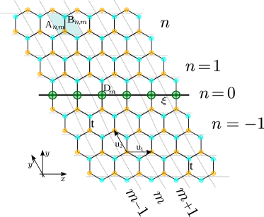
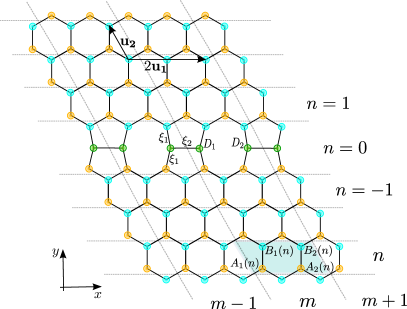
To illustrate the main physical issues and the method of approach, we start with a simplified version of a defect line, composed of a double line of pentagons oriented along the zigzag direction of the graphene lattice (see Fig. 1), which we dub as pentagon-only defect line. Compared to the more realistic linear defects that we treat later in the paper, the Lahiri et al. (2010) and the defects, it has the added simplicity of full translation symmetry along the defect direction, whereas the latter display a doubling of the unit cell along that same direction. The low-energy boundary conditions associated with these defect lines are also computed and compared with that of the pentagon-only defect line. Suitable choices of the microscopic parameters lead exactly to the same transmittance as a function of angle of incidence in all three cases. Finally, we also compute the conductance across a defect of length and find it to be proportional to at low temperatures, for all three defects considered.
II Electron transport across a pentagon-only grain boundary
II.1 The continuum description
A graphene plane with an extended line defect can be viewed in the low energy limit as two half-planes of massless Dirac Fermions, which cannot be joined smoothly, because of the defect, a line of discontinuity. To approach this problem, consider a finite strip of width in the direction, where there is a general local potential, , for such that as . Integrating the Dirac equation in the coordinate, the resultant general boundary condition for the Dirac spinor has the form (see Appendix A)
| (1) |
where the matrix reads
| (2) |
and This boundary condition has to satisfy the conservation of current in the direction, i.e., for any spinor, which implies that ; the form given in Eq. 2 satisfies this condition. An important feature, borne out by the derivation of Appendix A, is energy independence of the boundary condition. When we integrate the Dirac equation across the strip, and take the limit , the term containing the energy of the state, which, unlike the potential, is fixed, drops out.
An incoming wave from , will be partly reflected and partly transmitted at the defect. As a consequence, the real-space wave-function on each side of the defect line is given by
| (3c) | |||||
| (3f) | |||||
| (3i) | |||||
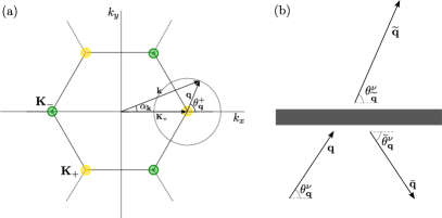
where specifies the Dirac cone, is the complex phase of , and , the complex phase of (see Fig. 3). The sign of the energy is noted by . Imposing the general boundary condition gives immediately the following general expression for the transmission probability
where we used the property , which follows from the condition of flux conservation, . A noteworthy feature, that follows naturally from this formulation, is the energy independence of the transmission across the defect.
To determine the actual values do the matrix elements of for a specific defect in a graphene lattice we must consider its microscopic description.
II.2 The low energy limit of tight binding
The first-neighbor TB Hamiltonian of graphene with a pentagon-only defect line (see Fig. 1), can be written as the sum of three terms, , where () stands for the Hamiltonian above (below) the defect line, while the remaining term, , describes the defect line itself. In second quantization the explicit forms of and read
| (5) | |||||
where for () (). The term describing the defect, , is
| (6) | |||||
where is the usual hopping amplitude of pristine graphene and is the hopping amplitude between the atoms of the defect line, as represented in Fig. 1.
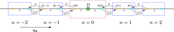
If we Fourier transform the Hamiltonian along the zigzag direction (-direction), we reduce it to an effective one-dimensional chain with two atoms per unit cell and a localized defect at its center (see Fig. 2).
The Hamiltonian of the effective chain is defined as
| (7) |
where the three terms on the right hand side of Eq. (7) read
| (8a) | |||||
| (8b) | |||||
The one-dimensional chain has alternating hopping amplitudes between the atoms, and . Moreover, the electron at a atom acquires an on-site energy term, , which depends on the value of the longitudinal momentum .
At the bulk of the one-dimensional chain ( and ), the TB equations for unit cell involve amplitudes at three different positions, , and ,
| (9a) | |||||
| (9b) | |||||
Nevertheless, replacing in Eq. (9a), we can solve these equations for and and recast them as a recurrence relation relating amplitudes at unit cell with those at unit cell ,
| (10) |
where . The passage matrix, , is given by
| (13) |
The eigenvectors of matrix with eigenvalues with , correspond to Bloch solutions propagating along the one-dimensional chain (band states). The eigenvectors with eigenvalues correspond to evanescent states which decrease when () when ().
Note that the previous formulation of the TB problem, is entirely equivalent to the usual one, where translational symmetry along the lattice vectors directions, allows the use of Bloch theorem to compute the eigenvectors and eigenvalues of the TB Hamiltonian for pristine graphene.
A similar construction to that of Eq. (10) can be carried out in the rows containing the defect. The TB equations for the defect and its neighbors in the one-dimensional chain are easily read from Fig. 2
| (14a) | |||||
| (14b) | |||||
| (14c) | |||||
| (14d) | |||||
| (14e) | |||||
where , to account for a possible potential difference between the two grains separated by the pentagon-only defect line. This set of TB equations can be used to construct a matrix equation relating the TB amplitudes in opposite sides of the defect. The technique is to solve each equation for the amplitude of the rightmost site in Fig. 2 and then cast them as matrix equations. For instance, Eq. (14a) is equivalent to
| (21) |
With this procedure, one can derive
| (22) |
where
is a matrix; is the Pauli matrix, used to switch rows, , and , and are
| (24c) | |||||
| (24f) | |||||
| (24i) | |||||
Note that the boundary condition matrix, [see Eq. (22)], depends on the energy, , on the longitudinal momentum, , and on the potential difference , through and .
We now have all the ingredients needed to compute the scattering coefficients of an electron wave by the pentagon-only defect line. Given an incoming wave from , the presence of the defect (line) at , produces a reflected and a transmitted component. In such a case, the wave-functions on each side of the defect (line) are given by
| (25a) | |||||
| (25b) | |||||
where and are, respectively, the reflection and transmission scattering amplitudes, and and stand for the right and left moving eigenstates of matrix , the passage matrix for pristine graphene, with corresponding eigenvalues noted by and . Imposing the boundary condition, Eq. (22), it is straightforward to obtain the coefficients and for a given energy and a given longitudinal momentum. In particular, reads
| (26) |
| where is the boundary condition matrix [see Eq. (22)] in the eigenbasis of the passage matrix of pristine graphene . The transmission probability is given by since flux conservation again requires that . |
But our main concern is the low energy limit. In the following we assume . Let us consider in parallel the equations that propagate the state in the bulk and in the defect:
| (27e) | ||||
| (27j) |
As is well known, near a Dirac point , the slowly varying Dirac spinor is defined by (ignoring irrelevant normalization constants)
| (30) |
and for a plane wave along
| (33) | |||||
| (34) |
where . This allows us to recast Eqs. (27e) and (27j) in terms of the Dirac fields,
| (35a) | ||||
| (35b) | ||||
where .
If we take the Fourier transform with respect to the spatial variable along in Eq. (35a),
| (36) |
In Appendix B we show that the matrix multiplying on the right hand side tends to the identity matrix when ; if we expand the right hand side to linear order in and , we obtain, as we should, the Dirac-Weyl equation (see Appendix B). However, at the defect, we find
| (39) |
which gives rise to the following equation
| (42) |
After Fourier transforming the previous equation in , and as the continuum approximation yields in , near the Dirac point, we end up concluding that the defect introduces a discontinuity in the Dirac fields of the form we derived from general considerations, , with
| (43) |
The transmission probability, given by the general expression of Eq. (LABEL:eq:trans-prob), becomes here
| (44) |
In Fig. 4, we plot the transmission probability , in terms of the angle of incidence on the defect line, for both the TB and the continuum approximation (CA), with . The various plots refer to different energies, but always to the same Dirac point (). As expected, the lower the energy, the better the agreement between the TB and the CA results. For the other Dirac point, the results are mirror-symmetric relatively to the normal incidence angle .
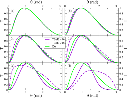
A special case is of some interest, namely, for low energies, , and , the transmission probability becomes , in which case the pentagon-only defect line acts as a valley filter, for angles of incidence close to . This same feature has been found in another type of defect, the , which we consider in the next section, by Gunlycke and White;Gunlycke and White (2011) this is no accident; we will show that these two defects share the same low energy limit.
It is worth noting, that since the passage matrix in the continuum limit is obtained with and , it is easily got in a back of envelope calculation, by writing and solving the TB equations at zero energy. This procedure is carried out in Appendix C.
It is expected that defect lines and grain boundaries in graphene are reactive,Malola et al. (2010) being a likely location for adsorption of atoms or molecules. Such adsorbates, are expected to locally perturb the properties of the defect lines. For simplicity, we may assume that the adsorbate only modifies the local energy at the atom it adsorbs to. We can account for such a phenomenon in the pentagon-only defect line, including in its TB model, an on-site energy, at the atoms of the defect line (see Fig. 1 or Fig. 2). Such a modification of the TB model, will necessarily modify the TB boundary condition matrix, [see Eq. (22)], as well as the continuum approximation one, [see Eq. (43)]. The TB boundary condition matrix, [see Eqs. (24)], will have its term modified. This will now include the on-site energy, , as . In the CA limit, the boundary condition matrix, , will have in the entry of the matrix instead of . Thus, the adsorption of molecules at the defect line, in very low energies, will be equivalent to rescaling the hopping between the atoms at the defect line.
III The and the defect lines
We now extend this treatment to the case of a defect lineLahiri et al. (2010); Gunlycke and White (2011); Jiang et al. (2011) (see Fig. 5), and of a defect line (see Fig. 6).
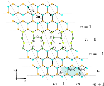
We can proceed in close analogy with the case of a pentagon-only defect line treated in the previous section. But these more realistic defects exhibit a feature that is not present in the previous case, namely, the doubling of the unit cell in the direction parallel to the defect. The corresponding folded First Brillouin Zone (FBZ) has twice as many states at the same Bloch wave vector, as in the original FBZ of graphene; the real space unit cell has two () and two () sites. Around the new Dirac points, now located at , there will be, in addition to two low-energy Dirac cones, two high energy bands.Rodrigues et al. (2011) At low energies, , the extra states show up as evanescent solutions.van Ostaay et al. (2011); Rodrigues et al. (2012)
In pristine graphene we know the form of the high and low energy modes since they are Bloch states of different wave vectors in the unfolded Brillouin zone. We can use this to define a change of basis that decouples, in the bulk, these two energy sectors ():
| (53) |
with
| (58) |
Defining
we have, , where the matrix , written in blocks of matrices, is
| (62) |
The and amplitudes propagate independently; and , the passage matrices associated with the high and the low-energy TB modes, are
| (63c) | |||||
| (63f) | |||||
The above computations are due to appear in a companion paperRodrigues et al. (2012) devoted to the study of these same systems under the TB approach.
In parallel with what we have done for the pentagon-only defect line [see Eqs. (14)- (24)], using the TB equations at the or at the defect lines, it is possible to write an expression relating amplitudes at the two sides of these defects, . The matrix is now a matrix relating the four amplitudes at each side of the defect line, and admixing, in general, high and low-energy modes of different sides of the defect. The high energy sector passage matrix in the bulk near and is
| (64) |
The corresponding eigenstates are evanescent, one growing exponentially as , localized on the sub-lattice, and the other decreasing as , localized in the sub-lattice. This same result was obtained by Ostaay et al. in the scope of the total reconstruction of the zigzag edge by Stone-Wales defects.van Ostaay et al. (2011)
Given this, we conclude that a low energy state, must have the following form in each one of the sides of the defect
| (65e) | |||||
| (65j) | |||||
This form fixes the amplitude, in terms of the low energy amplitudes and , since
and leads to an effective boundary condition relation for the low energy amplitudes only. The latter reads
| (71) |
where the effective boundary condition matrix is obtained from matrix
| (74) |
The low energy sector, with the matrix , can be analyzed exactly as was done in Appendix B for the pentagon only boundary. We define the Dirac fields as before,
| (78) |
so that, in the bulk
With a procedure entirely similar to the one detailed in Appendix B, one finds, after Fourier transforming in , that satisfies the Dirac equation. At the defect,
The calculation of yields
| (81) |
and so the boundary condition for the Dirac fields is
| (82) |
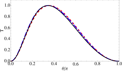
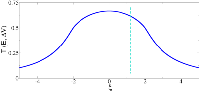
It is remarkable that this has exactly the same form as found in the pentagon–only boundary (c.f. Eq. [43]); the low energy transmission probabilities of these two line defects are the same provided In Fig. 7 we compare the transmission probabilities calculated with a full TB calculation for different values of and but the same value of ,Rodrigues et al. (2012) and the corresponding low energy approximation.
The treatment of the line defect presents no further novelty. Using the quick derivation method outlined in Appendix C, we arrive at the following passage matrix for the Dirac fields
| (85) |
where , and (see Fig 6 for the notation of the hopping amplitudes). The form of the passage matrix (and the transmission probability) is not identical to the previous cases, unless .
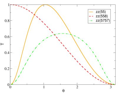
Despite the similarities, for general values of the hopping parameters, the transmittances originating from each of the defect lines can be considerably different. Such a case can be seen in Fig. 8, where we compare the low-energy transmission probabilities associated with each one of the previously discussed defect lines, for a special situation with all hopping amplitudes equal to , the bulk nearest neighbor amplitude.
IV Conductance
In this section we address the calculation of the linear conductance, across a line defect, and show that the energy independence of the transmission probability at low energies found in the previous three cases gives rise to a conductance linear in .
We make the usual assumption that the electron reservoirs at each side of the defect line are in equilibrium and are thus described by the single particle Fermi-Dirac distribution. Then the expression for the total net current across the defect line, associated with electrons living around the Dirac point , is given by
| (86) | |||||
where , stands for the spin degeneracy, is the potential difference between the each side of the defect line (see Fig. 1), and the Fermi-Dirac distribution function for chemical potential ; is the difference between chemical potentials at the two grains. In addition, stands for an angle-integrated transmission probability,
| (87) |
The total current is obtained summing the currents associated with the two Dirac points . One can verify that , and thus, , where is the valley degeneracy.
The conductance is then given by , where is the length of the defect line, when the current is in the linear regime,
| (88) |
where . The transmission probability, , does not depend on , as was seen above; it does depend on the values of the hopping amplitudes in the vicinity of the defect, through the passage matrix. [see Fig. 9 , for the case of the pentagon only defect]. We obtain,
| (89) |
where the function is a Fermi integral, , with limits , and for . The conductance is linear in temperature for ; in the opposite limit, , it is practically temperature independent,
| (90) | |||||
V Conclusion
In this text we have focused on the study of the low-energy continuum limit behavior of the electronic transport across periodic defect lines oriented along the zigzag direction of graphene. We have argued that in this limit, such extended defects essentially act as one-dimensional infinitesimally thin lines, that separate two regions governed by the Dirac Hamiltonian. In the low-energy continuum limit the defective line imposes a boundary condition on the Dirac spinors at each side of the defect. It is this boundary condition that defines the low-energy behavior of the electronic transport of such systems. We have demonstrated how can the boundary condition valid in the low-energy limit be computed from the TB description of the defect line.
We have presented such a reasoning while working out the problem of the electronic transport across a pentagon-only defect line, finding its transmittance to be energy independent. Furthermore, we have also studied two other kinds of more realistic periodic defect lines: the defect line, recently observed in graphene sheets,Lahiri et al. (2010) and the defect line. We have briefly examined these latter cases, emphasizing the fact that their periodicity forces the appearance of high-energy modes at the Dirac points in addition to the typical low-energy Dirac modes. It has been shown that the influence of the former, can be encompassed in an effective boundary condition seen by the low-energy massless Dirac fermions. The transmittance originating from such boundary conditions was again found to be energy independent. Furthermore, we have pointed out that the effective boundary conditions arising from the and defect lines, turn out to be similar to the one arising from the pentagon-only defect line. Moreover, the former can be mapped into the latter by an appropriate choice of the hopping parameters at the defects.
It is important to note that by expressing the transmission probability in terms of the boundary conditions satisfied by the Dirac fields at the defect, these results cast some light on the low-energy limit of the full TB calculations,Jiang et al. (2011) leaving us with a better understanding of the physics underlying such systems.
We have in addition shown how can we compute the low-energy limit conductance expression, across this kind of defect lines. Interestingly, at low temperatures, the conductance across a defect line of size , turned out to be linear in . This feature originates from the energy independence of the low-energy transmittance of our defect lines.
Finally, we must mention, that the procedures presented in this text, can be used to solve more complex scattering problems in graphene. Not only linear and periodic defect lines, but also periodic curvilinear extended defects oriented along graphene’s zigzag direction, can be worked out using the framework presented in this text.
Acknowledgements.
J. N. B. R. was supported by Fundação para a Ciência e a Tecnologia (FCT) through Grant No. SFRH/BD/44456/2008. N. M. R. P. was supported by Fundos FEDER through the Programa Operacional Factores de Competitividade - COMPETE and by FCT under project no. PEst-C/FIS/UI0607/2011. J. M. B. L. S. was supported by Fundacão para a Ciência e a Tecnologia (FCT) and is thankful for support and hospitality of Boston University and of National University of Singapore.Appendix A The general low-energy boundary condition for a defect line oriented along graphene’s zigzag direction
In this appendix we derive Eq. (2), determining the general form of the boundary condition matrix of a zigzag oriented defect line in the continuum limit.
Suppose that our defect line is located in the region defined by . Assume then, that in this region, we have a constant potential term in the Dirac equation of the form
| (91) |
Our aim is to consider the limit where when so that we can obtain the boundary condition of the defect line in the continuum limit. We must refer that there are some works published on the literature, considering the electronic scattering across regions with potentials that are a particular form of that given in Eq. 91.Katsnelson et al. (2006); Viana Gomes and Peres (2008)
The Dirac equation in the region of the potential is
Since the defect line is oriented along the -direction, we can choose
| (93) |
which, after substitution into Eq. (LABEL:eq:DrcEqPotGen), results in
| (94) |
where the operator reads
| (95) |
This first order differential equation (94) can be straightforwardly integrated,
| (96) |
Taking now the limit when , we obtain the following expression for the continuum limit of the boundary condition of a zigzag oriented defect line
| (97) |
As a final comment, we must stress the fact that the remaining terms in , namely and , do not contribute to the boundary condition when we take this limit; they are fixed in value, unlike the potential terms, and cannot give rise to a discontinuity when .
Appendix B Dirac equation from the passage matrix
In this appendix, we show how the Dirac-Weyl equation can be obtained from the low-energy passage matrix relation in Eq. (36)
| (98) |
Since ,
| (99) |
As we are working out a theory valid around the Dirac points, and are small, and we can thus expand the exponential, keeping solely the first order terms in the momentum,
| (102) | |||||
| (107) |
where is the identity matrix. This term cancels the one in the right hand side of Eq. (99) and we are left with
| (112) |
Upon multiplying by , we obtain Dirac’s equation,
| (114) |
where , with the usual notation of identifying the Dirac point.
Appendix C Quick derivation of the continuum limit boundary condition for the pentagon-only defect
In this brief appendix, we will present a quick derivation of the pentagon-only defect low-energy boundary condition ( and ), Eq. (43).
Let us start from the TB equations at the pentagon-only defect, Eqs. (14). In these equations, we begin by setting . In this way, the TB equations at the defect now read
| (115a) | |||||
| (115b) | |||||
| (115c) | |||||
| (115d) | |||||
| (115e) | |||||
where . From now on, we set ourselves at . The five equations written in Eqs. (115), contain 7 amplitudes, and we can solve them all in terms of and ; we obtain for and ,
| (122) |
which, using Eq. (35b), immediately identifies the passage matrix for the Dirac fields, Eq. (43).
This procedure is quite general, and can be applied to the the other line defects considered in this paper. In that case, however, we must express the TB amplitudes in terms of the amplitude of the low and high energy modes and set to zero the evanescent amplitudes of the states that grow on each side of the defect. We can then solve for the low energy amplitudes on one side of the defect, and obtain directly the passage matrix for the propagating modes.
References
- Li et al. (2009) X. Li, W. Cai, J. An, S. Kim, J. Nah, D. Yang, R. Piner, A. Velamakanni, I. Jung, E. Tutuc, et al., Science 324, 1312 (2009).
- Reina et al. (2009) A. Reina, X. Jia, J. Ho, D. Nezich, H. Son, V. Bulovic, M. S. Dresselhaus, and J. Kong, Nano Lett. 9, 30 (2009).
- Kim et al. (2009) K. S. Kim, Y. Zhao, H. Jang, S. Y. Lee, J. M. Kim, K. S. Kim, J.-H. Ahn, P. Kim, J.-Y. Choi, and B. H. Hong, Nature 457, 706 (2009).
- Bae et al. (2010) S. Bae, H. Kim, Y. Lee, X. X. andJae Sung Park, Y. Zheng, J. B. andTian Lei, H. R. Kim, Y. I. Song, Y.-J. Kim, K. S. Kim, et al., Nature Nanotechnology 5, 574 (2010).
- Huang et al. (2011) P. Y. Huang, C. S. Ruiz-Vargas, A. M. van der Zande, W. S. Whitney, M. P. Levendorf, J. W. Kevek, S. Garg, J. S. Alden, C. J. Hustedt, Y. Zhu, et al., Nature 469, 389 (2011).
- Kim et al. (2011) K. Kim, Z. Lee, W. Regan, C. Kisielowski, M. F. Crommie, and A. Zettl, ACS Nano 5, 2142 (2011).
- Nemes-Incze et al. (2011) P. Nemes-Incze, K. J. Yoo, L. Tapaszto, G. Dobrik, J. Labar, Z. E. Horvath, C. Hwang, and L. P. Biro, Appl. Phys. Lett. 99, 023104 (2011).
- Stone and Wales (1986) A. Stone and D. Wales, Chem. Phys. Lett. 128, 501 (1986).
- Meyer et al. (2008) J. Meyer, C. Kisielowski, R. Emi, M. Rossell, M. Crommie, and A. Zettl, Nano. Lett. 8, 3582 (2008).
- Lahiri et al. (2010) J. Lahiri, Y. Lin, P. Bozkurt, I. I. Oleynik, and M. Batzill, Nature Nanotechnology 5, 326 (2010).
- Ferreira et al. (2011) A. Ferreira, X. Xu, C. Tan, S. Bae, N. Peres, B. Hong, B. Ozyilmaz, and A. Castro Neto, EPL 94, 28003 (2011).
- Malola et al. (2010) S. Malola, H. Hakkinen, and P. Koskinen, Phys. Rev. B 81, 165447 (2010).
- Yazyev and Louie (2010a) O. V. Yazyev and S. G. Louie, Phys. Rev. B 81, 195420 (2010a).
- Grantab et al. (2011) R. Grantab, V. B. Shenoy, and R. S. Ruoff, Science 330, 946 (2011).
- Novoselov et al. (2004) K. S. Novoselov, A. K. Geim, S. V. Morozov, D. Jiang, Y. Zhang, S. V. Dubonos, I. V. Grigorieva, and A. A. Firsov, Science 306, 666 (2004).
- Novoselov et al. (2005) K. S. Novoselov, D. Jiang, T. Booth, V. V. Khotkevich, S. M. Morozov, and A. K. Geim, Proc. Natl. Acad. Sci. 102, 10451 (2005).
- Castro Neto et al. (2009) A. H. Castro Neto, F. Guinea, N. M. R. Peres, K. S. Novoselov, and A. K. Geim, Rev. Mod. Phys. 81, 109 (2009).
- Peres (2010) N. M. R. Peres, Rev. Mod. Phys. 82, 2673 (2010).
- Yazyev and Louie (2010b) O. V. Yazyev and S. G. Louie, Nature Materials 9, 806 (2010b).
- Bahamon et al. (2011) D. A. Bahamon, A. L. C. Pereira, and P. A. Schulz, Phys. Rev. B 83, 155436 (2011).
- Gunlycke and White (2011) D. Gunlycke and C. T. White, Phys. Rev. Lett. 106, 136806 (2011).
- Jiang et al. (2011) L. Jiang, X. Lv, and Y. Zheng, Phys. Lett. A 376, 136 (2011).
- Semenoff (1984) G. W. Semenoff, Phys. Rev. Lett. 53, 2449 (1984).
- Rodrigues et al. (2011) J. N. B. Rodrigues, P. A. D. Gonçalves, N. F. G. Rodrigues, R. M. Ribeiro, J. M. B. Lopes dos Santos, and N. M. R. Peres, Phys. Rev. B 84, 155435 (2011).
- van Ostaay et al. (2011) J. A. M. van Ostaay, A. R. Akhmerov, C. W. J. Beenakker, and M. Wimmer, Phys. Rev. B 84, 195434 (2011).
- Rodrigues et al. (2012) J. N. B. Rodrigues, N. M. R. Peres, and J. M. B. Lopes dos Santos, to be submitted (2012).
- Katsnelson et al. (2006) M. I. Katsnelson, K. S. Novoselov, and A. K. Geim, Nat. Phys. 2, 620 (2006).
- Viana Gomes and Peres (2008) J. Viana Gomes and N. M. R. Peres, Journal of Physics: Condensed Matter 20, 325221 (2008).