SISSA 23/2012/EP-FM

${\cal N}=2$ gauge theories on toric singularities,
blow-up formulae and $W$-algebrae

Giulio Bonelli^♡♠, Kazunobu Maruyoshi^♡, Alessandro Tanzini^♡ and Futoshi Yagi^♡

^♡SISSA and INFN, Sezione di Trieste, via Bonomea 265, 34136 Trieste, Italy
^♠ I.C.T.P. – Strada Costiera 11, 34014 Trieste, Italy

Abstract

We compute the Nekrasov partition function of gauge theories on the (resolved) toric singularities $\mathbb{C}^{2}/\Gamma$ in terms of blow-up formulae. We discuss the expansion of the partition function in the $\epsilon_{1},\epsilon_{2}\to 0$ limit along with its modular properties and how to derive them from the M-theory perspective. On the two-dimensional conformal field theory side, our results can be interpreted in terms of representations of the direct sum of Heisenberg plus $W_{N}$-algebrae with suitable central charges, which can be computed from the fan of the resolved toric variety. We provide a check of this correspondence by computing the central charge of the two-dimensional theory from the anomaly polynomial of M5-brane theory. Upon using the AGT correspondence our results provide a candidate for the conformal blocks and three-point functions of a class of the two-dimensional CFTs which includes parafermionic theories.

  e-mails: bonelli, maruyosh, tanzini, fyagi@sissa.it

1 Introduction

${\cal N}=2$ gauge theories in four-dimensions provide a seemingly inexhaustible source of results in theoretical physics and geometry. The partition function of the gauge theory on the so-called Omega background [1] with parameters $\epsilon_{1,2}$ gives the exact answer not only to the prepotential of the theory, summing over all the instanton contributions, in the leading behavior $\epsilon_{1,2}\rightarrow 0$, but also to the gravitational corrections included in finite $\epsilon$ terms. The introduction of the Omega background also enables us to concatenate ${\mathcal{N}}=2$ theories with two-dimensional conformal field theories (CFT) [2] and quantum integrable systems [3].

In this paper we present a systematic study of these theories on the minimal resolution $X_{p,q}$ of the toric singularities $\mathbb{C}^{2}/\Gamma_{p,q}$ with $\Gamma_{p,q}\subset U(2)$ a finite group. We compute the full Nekrasov partition function by reducing the problem to a diagrammatic algorithm related to the fan of the toric variety. We then analyze the geometry of the low-energy effective action and its modular properties, by studying the $\epsilon_{1,2}\to 0$ limit and by elucidating their M-theory origin. We find that there are two types of contributions, being related respectively to the regular and irreducible representations of $\Gamma_{p,q}$. The former is encoded in the Seiberg-Witten curve $\Sigma$ of the gauge theory on the flat space, up to an overall volume factor. The twisted sector is encoded in suitable modular functions whose lattice is determined by the intersection matrix of the Hirzebruch-Jung resolution of the singularity. Indeed we show that the twisted sector contribution can be written in term of blow-up equations which generalize the ones of [4, 5, 6] to the blow-up of singular points.

Let us observe that in general ${\cal N}=2$ theories can be formulated on any differentiable four-manifold by using a twisting procedure [7]. A cautionary remark is in order here: when $\Gamma$ is a Kleinian subgroup of $SU(2)$ the resolved manifold is an ALE space, which displays an hyper-kahler structure. Then the original and the twisted theory share the same energy-momentum tensor and are physically equivalent. For more general $\Gamma_{p,q}$ subgroups the resolved manifolds are only Kahler and preserve half of the supersymmetric charges with respect to the ALE case. The energy-momentum tensor is in this case substantially modified and only the twisted version of the theory preserves supersymmetry.

In section 2, the full partition function will be given and expanded in $\epsilon_{1,2}$ to see the geometric properties. Remarkably, the partition function is a nested product of $\mathbb{C}^{2}$ partition functions with arguments shifted according to the $X_{p,q}$ geometry. By studying the leading orders in the expansion we show that the low-energy effective action is encoded in the Seiberg-Witten curve and the intersection matrix of the resolved toric variety. We also discuss next to leading orders including gravitational corrections and the Nekrasov-Shatashvili limit of the full partition function.

In section 3, we consider the Nekrasov partition function on $X_{p,q}$ at classical, one loop, and instanton level, separately and we relate them with the blowup formula at each level.

In section 4, we provide a description of the system in terms of M5-branes on $X_{p,q}\times{\cal C}$ where ${\cal C}$ is a punctured Riemann surface. We discuss how the modular properties of the low-energy effective action are captured by the generalized elliptic index of the M5-brane system in the far infrared, where the system reduces to a single M5-brane wrapping the Seiberg-Witten curve $\Sigma$.

The M5-brane picture can be also used to gain some insights on the corresponding two-dimensional CFT à la AGT [2]. Indeed, our result for the full Nekrasov partition function indicates the emergence of representations of the algebra ${\cal A}_{N}(X_{p,q})$ given by direct sum of Heisenberg plus $W_{N}$ algebrae with suitable central charges which can be computed from the fan of the toric variety, see (5.2). On the other hand, the central charge of the candidate two-dimensional CFT can be computed from the anomaly polynomial of the $N$ M5-branes wrapping ${\cal C}$ via equivariant integration over the four-dimensional space [8, 9, 10]. In section 5, we check that this reproduces the overall central charge of the algebra ${\cal A}_{N}(X_{p,q})$.

We conclude in section 6 with various discussions. In the Appendices, we review the properties of $X_{p,q}$ spaces, collect useful formulae which are needed in the computation and expansion of the partition function and we explicitly give the first terms in the expansion of the instanton sum for the $U(2)$ SYM theory on $A_{2}$ ALE.

2 ${\cal N}=2$ gauge theories on toric singularities

The partition function of ${\cal N}=2$ $U(N)$ gauge theories can be computed via equivariant localization methods on a general toric manifold $X$. Indeed, one exploits the $({\mathbb{C}}^{*})^{2+N}$ action on the moduli space of instantons on $X$, where $({\mathbb{C}}^{*})^{2}$ is the lift of space-time automorphisms of $X$ to the instanton moduli space while $({\mathbb{C}}^{*})^{N}$ is the complexification of the Cartan torus of the $U(N)$ gauge symmetry. For compact toric rational surfaces this was studied in [11]. In this section we discuss open varieties focusing on the most general toric singularity $\mathbb{C}^{2}/\Gamma_{p,q}$, with $\Gamma_{p,q}\subset U(2)$ a finite group acting on local coordinates as $z_{1}\to e^{2\pi i/p}z_{1}$ and $z_{2}\to e^{2\pi iq/p}z_{2}$, with $(p,q)$ being coprime and $q<p$. More precisely we consider the minimal resolution of this singularity $X_{p,q}=\widetilde{\mathbb{C}^{2}/\Gamma_{p,q}}$, known as Hirzebruch-Jung resolution – see Appendix A for details. The $\mathcal{N}=4$ partition function for these geometries was calculated in [12, 13, 14, 15].

The general procedure to compute the ${\cal N}=2$ Nekrasov partition function is the following: any toric variety is described in terms of a fan encoding its patching structure as a complex manifold. In each patch the computation of the Nekrasov partition function reduces to the standard one in ${\mathbb{C}}^{2}$ spanned by suitable variables which provide a basis of invariants of the orbifold action $\Gamma_{p,q}$. One thus obtains a diagrammatic algorithm which computes the full partition function from the weights of the $({\mathbb{C}}^{*})^{N+2}$-torus action in each patch. Indeed, as it has been suggested in [16] and then shown in [17, 18, 19] for the blown-up $\mathbb{P}^{2}$ and $\mathcal{O}_{\mathbb{P}^{1}}(-2)$ cases, this description is particularly simple when one considers the full ${\cal N}=2$ partition function including the classical and perturbative contributions. The full partition function on the resolved toric singularity is simply given by the intertwined product of the full partition functions in each patch. More precisely, we propose that the ${\cal N}=2$ full Nekrasov partition function on $X_{p,q}$ is given by the blowup formula

$$Z^{X_{p,q}}_{{\rm full}}(\vec{a},\epsilon_{1},\epsilon_{2})=\sum_{\{\vec{k}^{(\ell)}\}}\prod_{\ell=0}^{L-1}Z^{{\mathbb{C}}^{2}}_{{\rm full}}(\epsilon_{1}^{(\ell)},\epsilon_{2}^{(\ell)},\vec{a}^{(\ell)})\xi_{\ell}^{c_{1}^{(\ell)}},$$ (2.1)

where $\vec{a}=\{a_{\alpha}\},\alpha=1,\ldots,N$ are the vev’s of the scalar field of the ${\cal N}=2$ vector multiplet,

$$a^{(\ell)}_{\alpha}=a_{\alpha}+k^{(\ell+1)}_{\alpha}\epsilon_{1}^{(\ell)}+k^{(\ell)}_{\alpha}\epsilon_{2}^{(\ell)}$$ (2.2)

and $k^{(0)}=k^{(L)}=0$.

The above formula (2.1) can be obtained as follows. As reviewed in Appendix A, the $X_{p,q}$ variety is described in terms of $L$ patches with local coordinates described in (A.2). These local coordinates transform under the $({\mathbb{C}}^{*})^{2}$ torus action with weights $\left(\epsilon_{1}^{(\ell)},\epsilon_{2}^{(\ell)}\right)$ whose explicit expression is given in (A.20). The fixed point data on $X_{p,q}$ are described in terms of a collection of Young tableaux $\{\vec{Y}_{\ell}\}$, and of rational numbers $\{\vec{k}^{(\ell)}\}$ $\ell=0,\ldots,L-1$ describing respectively the $({\mathbb{C}}^{*})^{N+2}$-invariant point-like instantons in each patch and the magnetic fluxes of the gauge field on the blown-up spheres which correspond to the first Chern class $c_{1}(E)$ of the gauge bundle $E$. More explicitly, the homology decomposition of the $c_{1}$ reads

$$c_{1}=-\sum_{\alpha,\ell}k_{\alpha}^{(\ell)}\Delta_{\ell},$$ (2.3)

where $\{\Delta_{\ell}\}$ is a basis of $H_{2}(X_{p,q})$. Since the $c_{1}$ has an integer decomposition in the dual cohomology basis

$$c_{1}=\sum_{\alpha,\ell}u_{(\ell)\alpha}\omega_{\ell}\ \ ,\vec{u}_{(\ell)}\in{\mathbb{Z}}^{N(L-1)},$$ (2.4)

where $\omega_{\ell}$ is a basis of $H^{2-}(X_{p,q})$ normalized by the condition $\int_{\Delta_{\ell}}\omega_{n}=\delta_{n}^{\ell}$, we get that $\vec{k}=C^{-1}\vec{u}$ where ${\cal I}_{p,q}\equiv-C$ is the intersection form of the resolved $X_{p,q}$ variety displayed in the Appendix A, eq.(A.1). Therefore, the lattice summation in (2.1) is $\{\vec{k}^{(\ell)}\}\in(\mbox{1}\mbox{l}_{N}\otimes C^{-1})\mathbb{Z}^{N(L-1)}$.

Note also that we have multiplied $\xi_{\ell}$ factors in order to keep track of the first Chern classes $c_{1}^{(\ell)}$ of the gauge bundle

$$c_{1}^{(\ell)}=\sum_{\alpha=1}^{N}u_{(\ell)\,\alpha}=\sum_{\alpha=1}^{N}\sum_{m=1}^{L-1}C_{\ell m}k^{(m)}_{\alpha}.$$ (2.5)

In other words, we are considering the expectation value $Z_{\rm full}^{X_{p,q}}=\left<e^{\frac{1}{2\pi}\sum_{\ell}z_{\ell}\int Tr(F)\wedge\omega_{(\ell)}}\right>$ with $\xi_{\ell}=e^{(C^{-1}z)^{(\ell)}}$, rather than the partition function.

The shift in the Cartan parameters (2.2) can be computed by the patch-to-patch relative shift of the $\left({\mathbb{C}}^{*}\right)^{N}$ weights which is induced by the non-trivial magnetic flux of the gauge field on the blown-up spheres as explained in the following. We denote the $\alpha$-th gauge field on the north patch as $(A_{N})_{(\ell)\alpha}$ while that on the south patch as $(A_{S})_{(\ell)\alpha}$ in the $\ell$-th blown up sphere ($\ell=1,\cdots,L-1$). At the equator, they coincide up to the gauge transformation

$$(A_{N})_{(\ell)\alpha}=(A_{S})_{(\ell)\alpha}+\partial_{\phi}\psi_{(\ell)\alpha}(\phi)$$ (2.6)

where $\phi$ is the coordinate along the equator. When we go around the equator, the phase is identified up to a multiple of $2\pi$:

$$\psi_{(\ell)\alpha}(\phi+2\pi)=\psi_{(\ell)\alpha}(\phi)-2\pi u_{(\ell)\alpha}$$ (2.7)

with $u_{(\ell)\alpha}\in{\mathbb{Z}}$ being the magnetic flux through the blown-up sphere $\Delta_{\ell}$

$$\frac{1}{2\pi}\int_{\Delta_{\ell}}F_{(\ell)\alpha}={u}_{(\ell)\alpha}.$$ (2.8)

According to (2.6) and (2.7) the non-trivial flux through the $\ell$-th blown-up sphere modifies the relative weights of the gauge $U(1)^{N}$ action $a^{(\ell)}_{\alpha}$ and $a^{(\ell-1)}_{\alpha}$ by $a^{(\ell)}_{\alpha}=a^{(\ell-1)}_{\alpha}-u_{(\ell)\alpha}\epsilon_{1}^{(\ell)}$. In order to get (2.2) we parametrize the weights of the Cartan action as seen from the first and last patches and impose consistency. The difference between $a^{(0)}_{\alpha}$ and $a_{\alpha}$ is proportional to $\epsilon^{(0)}_{1}=p\epsilon_{1}$,

$$a^{(\ell)}_{\alpha}=a_{\alpha}+x\epsilon_{1}-\sum_{m=1}^{\ell}u_{(m)\alpha}\epsilon_{1}^{(m)}.$$ (2.9)

Furthermore, the difference between $a^{(L-1)}_{\alpha}$ and $a_{\alpha}$ is proportional to $\epsilon_{2}^{(L-1)}=p\epsilon_{2}$. Henceforth, we obtain the condition

$$a^{(L-1)}_{\alpha}+y\epsilon_{2}=a_{\alpha}\,\,\Rightarrow\,\,x\epsilon_{1}-\sum_{m=1}^{L-1}u_{(m)\alpha}\epsilon_{1}^{(m)}+y\epsilon_{2}=0,$$ (2.10)

which determine the coefficients $x$ and $y$ as

$$x=-\sum_{\ell=1}^{L-1}(pq_{\ell}-qp_{\ell})u_{(\ell)\alpha},\qquad y=-\sum_{\ell=1}^{L-1}p_{\ell}u_{(\ell)\alpha}.$$ (2.11)

By using this result one gets (2.2) as explained in detail at the end of Appendix B.

Due to the asymmetric nature of the $\Gamma_{p,q}$ orbifold, the usual symmetry $\epsilon_{1}\leftrightarrow\epsilon_{2}$ appearing in the flat $\mathbb{C}^{2}$ case is now replaced by the invariance of the full partition function under the simultaneous exchange $q\leftrightarrow p_{L-1}$. This in turn is the reversal of the continuous fraction $[e_{1},\ldots,e_{L-1}]\leftrightarrow[e_{L-1},\ldots,e_{1}]$ and pictorially corresponds to reverse the order of the chain of blown-up spheres.

2.1 Blowup formulae and theta functions

In this subsection, we discuss the behavior of the Nekrasov partition function on $X_{p,q}$ in the limit $\epsilon_{1,2}\to 0$. As we will show, this enables us to uncover the modular properties of the ${\cal N}=2$ partition function and to derive a generalization of the blow-up equations for the Donaldson polynomials [4, 6] to the case of toric singularities.

First of all, we expand the full partition function on $\mathbb{C}^{2}$ as

$$-\epsilon_{1}\epsilon_{2}\ln Z^{\mathbb{C}^{2}}_{{\rm full}}(\epsilon_{1},\epsilon_{2},\vec{a},q)\equiv F_{\Omega}(\epsilon_{1},\epsilon_{2},\vec{a},q)$$

$$\equiv F_{0}(\vec{a},q)+(\epsilon_{1}+\epsilon_{2})H(\vec{a},q)+\epsilon_{1}\epsilon_{2}F_{1}(\vec{a},q)+(\epsilon_{1}+\epsilon_{2})^{2}G(\vec{a},q)+\mathcal{O}(\epsilon^{3}).$$ (2.12)

Note that these include the classical and the perturbative part. The leading part $F_{0}(\vec{a},q)$ is the prepotential and related to the IR effective gauge coupling constant as

$$\left(\tau^{\mathbb{C}^{2}}_{\rm eff}\right)^{\alpha\beta}\equiv\partial^{\alpha}\partial^{\beta}F_{0}(\vec{a},q).$$ (2.13)

By substituting the expansion (2.12) into each of the $Z^{\mathbb{C}^{2}}$ factors in the blowup formula (2.1), we obtain

$$-\ln Z^{\mathbb{C}^{2}}_{{\rm full}}(\epsilon_{1}^{(\ell)},\epsilon_{2}^{(\ell)},\vec{a}+\epsilon_{1}^{(\ell)}\vec{k}^{(\ell+1)}+\epsilon_{2}^{(\ell)}\vec{k}^{(\ell)})$$ (2.14)

$$= \frac{1}{\epsilon_{1}^{(\ell)}\epsilon_{2}^{(\ell)}}F_{0}(\vec{a},q)+\frac{\epsilon_{1}^{(\ell)}+\epsilon_{2}^{(\ell)}}{\epsilon_{1}^{(\ell)}\epsilon_{2}^{(\ell)}}H(\vec{a},q)+\frac{\epsilon_{1}^{(\ell)}k^{(\ell+1)}_{\alpha}+\epsilon_{2}^{(\ell)}k^{(\ell)}_{\alpha}}{\epsilon_{1}^{(\ell)}\epsilon_{2}^{(\ell)}}\partial^{\alpha}F_{0}(\vec{a},q)$$ (2.15)

$$+F_{1}(\vec{a},q)+\frac{(\epsilon_{1}^{(\ell)}+\epsilon_{2}^{(\ell)})^{2}}{\epsilon_{1}^{(\ell)}\epsilon_{2}^{(\ell)}}G(\vec{a},q)+\frac{(\epsilon_{1}^{(\ell)}+\epsilon_{2}^{(\ell)})(\epsilon_{1}^{(\ell)}k^{(\ell+1)}_{\alpha}+\epsilon_{2}^{(\ell)}k^{(\ell)}_{\alpha})}{\epsilon_{1}^{(\ell)}\epsilon_{2}^{(\ell)}}\partial^{\alpha}H(\vec{a},q)$$ (2.16)

$$+\left(\tau^{\mathbb{C}^{2}}_{\rm eff}\right)^{\alpha\beta}\frac{(\epsilon_{1}^{(\ell)}k^{(\ell+1)}_{\alpha}+\epsilon_{2}^{(\ell)}k^{(\ell)}_{\alpha})(\epsilon_{1}^{(\ell)}k^{(\ell+1)}_{\beta}+\epsilon_{2}^{(\ell)}k^{(\ell)}_{\beta})}{\epsilon_{1}^{(\ell)}\epsilon_{2}^{(\ell)}}+\mathcal{O}(\epsilon^{3}).$$ (2.17)

Then, we need to sum over $\ell$. By using the identities in Appendix B and by comparing with original partition function on $\mathbb{C}^{2}$, we obtain the following result up to terms of order one in $\epsilon_{1},\epsilon_{2}$ in the exponential

$$Z_{\rm full}^{X_{p,q}}(\epsilon_{1},\epsilon_{2},\vec{a},q)\simeq\left(Z_{\rm full}^{\mathbb{C}^{2}}(\epsilon_{1},\epsilon_{2},\vec{a},q)\right)^{\frac{1}{p}}\exp\left[\left(-L+\frac{1}{p}\right)F_{1}(\vec{a},q)+N_{G}G(\vec{a},q)\right]$$ (2.18)

$$~{}~{}~{}~{}~{}~{}~{}\times\sum_{\{\vec{k}^{(\ell)}\}}\xi_{\ell}^{c_{1}^{(\ell)}}\exp\left[\frac{1}{2}\sum_{\ell,m=1}^{L-1}\sum_{\alpha,\beta=1}^{N}k_{\alpha}^{(\ell)}C_{\ell m}\left(\tau_{\rm eff}^{\mathbb{C}^{2}}\right)^{\alpha\beta}k_{\beta}^{(m)}+\sum_{\alpha=1}^{N}\sum_{\ell=1}^{L-1}(e_{\ell}-2)k_{\alpha}^{(\ell)}\partial_{\alpha}H\right],$$

where

$$N_{G}=\frac{p_{L-1}+q+2}{p}-2L+\sum_{\ell=1}^{L-1}e_{\ell}.$$ (2.19)

$p_{L-1}$ and $e_{\ell}$ are defined in Appendix A.

The above result shows that the leading term in the $\epsilon_{1,2}\rightarrow 0$ limit is simply the same as the gauge theory prepotential on $\mathbb{C}^{2}$ up to a factor $p$

$$Z_{\rm full}^{X_{p,q}}=\exp\left(-\frac{F_{0}}{p\epsilon_{1}\epsilon_{2}}+\ldots\right).$$ (2.20)

This can be interpreted as follows: the low energy effective theory has a sector which is described by the very same Seiberg-Witten curve $\Sigma$ and differential $\lambda_{{\rm SW}}$ as the flat space. However, the volume factor is rescaled by the order of the quotient group. This sector corresponds to point-like instantons sitting in the regular representation of $\Gamma_{p,q}$. These probe the whole quotient space $X_{p,q}$ and their contribution is weighted by the equivariant volume. Besides this sector, there is also the one of instantons in the irreducible representation of the finite group. These are stuck at the invariant loci of the orbifold action, namely on the blown-up spheres, and as such their contribution is independent on $\epsilon_{1},\epsilon_{2}$. This contribution is fully characterized by the intersection matrix of $X_{p,q}$ as displayed in the second line of (2.18). The subleading terms in the first and second lines of (2.18) represent the gravitational couplings.

One can check that the same behavior holds in the NS limit $\epsilon_{2}\to 0$ with $\epsilon_{1}$ finite [3]. In particular, regular instantons contribute as follows

$${\mathcal{W}}^{X_{p,q}}(\vec{a},\epsilon_{1})\equiv-\lim_{\epsilon_{2}\rightarrow 0}p\epsilon_{2}\ln Z^{X_{p,q}}_{{\rm full}}={\mathcal{W}}^{\mathbb{C}^{2}}(\vec{a},\epsilon_{1}),$$ (2.21)

where we redefined the limit in terms of the equivariant volume of the orbifold. This can be derived in the following way. In the full partition function (2.1) the only part which contributes to this limit is the one with $\ell=L-1$, because the only possibility to get $\frac{1}{\epsilon_{2}}$ behavior in the exponential is this case as can be seen from the explicit form of $\epsilon_{1,2}^{(\ell)}$ (A.21). Then, we see that $Z^{\mathbb{C}^{2}}_{{\rm full}}(\epsilon_{1}^{(L-1)},\epsilon_{2}^{(L-1)},\vec{a}^{(L-1)})=\exp(\frac{1}{p\epsilon_{2}}F_{\Omega}(\epsilon_{1},0,\vec{a}))$, which leads to (2.21).

2.1.1 ALE space

In this subsection, we consider the expansion (2.18) in the case of the ALE space. The $A_{p}$ ALE space corresponds to $X_{p,p-1}$. In this case, we have

$$Z^{\rm ALE}_{{\rm full}}(\epsilon_{1},\epsilon_{2},\vec{a},q) \simeq\left(Z^{\mathbb{C}^{2}}_{{\rm full}}(\epsilon_{1},\epsilon_{2},\vec{a},q)\right)^{\frac{1}{p}}\exp\left[\left(-p+\frac{1}{p}\right)F_{1}(\vec{a},q)\right]$$ (2.22)

$$\times\sum_{\{\vec{k}^{(\ell)}\}}\xi_{\ell}^{c_{1}^{(\ell)}}\exp\left[\frac{1}{2}\sum_{\ell,m=1}^{p-1}\sum_{\alpha,\beta=1}^{N}k_{\alpha}^{(\ell)}C_{\ell m}\left(\tau_{\rm eff}^{\mathbb{C}^{2}}\right)^{\alpha\beta}k_{\beta}^{(m)}\right],$$ (2.23)

since $e_{\ell}=2$ for all $\ell$ and $N_{G}=0$.

For illustration, let us consider $A_{1}$, where the expansion is

$$Z^{\rm A_{1}}_{{\rm full}}(\epsilon_{1},\epsilon_{2},\vec{a},q) \simeq Z^{\mathbb{C}^{2}}_{{\rm full}}(\epsilon_{1},\epsilon_{2},\vec{a},q)^{\frac{1}{2}}e^{-3F_{1}(\vec{a},q)/2}\sum_{\{\vec{k}\}}\xi^{c_{1}}\exp\left[\sum_{\alpha,\beta=1}^{N}k_{\alpha}\left(\tau_{\rm eff}^{\mathbb{C}^{2}}\right)^{\alpha\beta}k_{\beta}\right].$$ (2.24)

Note that in this case $k_{\alpha}$ is integer or half-integer. So far, we did not specify which gauge theory we were considering. Now, let us analyze ${\cal N}=2^{*}$ gauge theory with gauge group $U(2)$. We write $F_{0}$ as

$$F_{0}=\pi i\tau_{cl}\sum_{i=1,2}a_{i}^{2}+\tilde{F}_{0},$$ (2.25)

where $\tilde{F}_{0}$ includes the one-loop and instanton contributions, while the first term is the classical one. Since $\tilde{F}_{0}$ only depends on the difference $a_{1}-a_{2}$ in this theory, we can write the coupling constant term as

$$k_{\alpha}k_{\beta}(\tau_{{\rm eff}}^{\mathbb{C}^{2}})^{\alpha\beta}=k_{\alpha}k_{\beta}\partial^{\alpha}\partial^{\beta}F_{0}=\pi i\tau_{{\rm cl}}k_{+}^{2}+\pi i\tau_{{\rm eff}}k_{-}^{2},$$ (2.26)

where $k_{\pm}=k_{1}\pm k_{2}$ and we have defined $\tau_{{\rm eff}}=\tau_{{\rm cl}}+\frac{1}{\pi i}\frac{\partial^{2}}{\partial a_{-}^{2}}\tilde{F}_{0}$ with $a_{\pm}=a_{1}\pm a_{2}$. Therefore we can rewrite (2.24) as

$$Z^{\rm A_{1}}_{{\rm full}} \simeq (Z^{\mathbb{C}^{2}}_{{\rm full}})^{\frac{1}{2}}e^{-3F_{1}/2}\sum_{\{\vec{k}\}}\xi^{2k_{+}}e^{\pi i\tau_{{\rm cl}}k_{+}^{2}}e^{\pi\tau_{{\rm eff}}ik_{-}^{2}}$$ (2.27)

$$= (Z^{\mathbb{C}^{2}}_{{\rm full}})^{\frac{1}{2}}e^{-3F_{1}/2}\left(\vartheta_{3}(q_{{\rm cl}};\xi^{2})\vartheta_{3}(q_{{\rm eff}};1)+\vartheta_{2}(q_{{\rm cl}};\xi^{2})\vartheta_{2}(q_{{\rm eff}};1)\right),$$

where $q_{{\rm cl}}=e^{\pi i\tau_{{\rm cl}}}$ and $q_{{\rm eff}}=e^{\pi i\tau_{{\rm eff}}}$ and

$$\vartheta_{3}(q;x)=\sum_{n\in\mathbb{Z}}q^{n^{2}}x^{n},~{}~{}~{}~{}\vartheta_{2}(q;x)=\sum_{n\in\mathbb{Z}}q^{(n-1/2)^{2}}x^{n-1/2}.$$ (2.28)

It is interesting to consider the above results for fixed first Chern class. For even $c_{1}$, the first term of the r.h.s. of (2.27) contributes as

$$\frac{Z_{{\rm full}}^{c_{1}=even}}{(Z^{\mathbb{C}^{2}}_{{\rm full}})^{1/2}}\simeq q_{{\rm eff}}^{\frac{c_{1}^{2}}{4}}e^{-3F_{1}/2}\vartheta_{3}(q_{{\rm eff}}).$$ (2.29)

For odd $c_{1}$, we get

$$\frac{Z_{{\rm full}}^{c_{1}=odd}}{(Z^{\mathbb{C}^{2}}_{{\rm full}})^{1/2}}\simeq q_{{\rm eff}}^{\frac{c_{1}^{2}}{4}}e^{-3F_{1}/2}\vartheta_{2}(q_{{\rm eff}}).$$ (2.30)

These provide blow-up formulae for singular points.

2.1.2 ${\mathcal{O}}_{\mathbb{P}^{1}}(-p)$ space

We consider in this subsection the ${\mathcal{O}}_{\mathbb{P}^{1}}(-p)$ space, that is $X_{p,1}$. Since in this case there are two patches $L=2$ and $e=p$ as can be seen in Appendix A, the expansion (2.18) becomes

$$Z_{\rm full}^{X_{p,1}}(\epsilon_{1},\epsilon_{2},\vec{a},q)\simeq\left(Z_{\rm full}^{\mathbb{C}^{2}}(\epsilon_{1},\epsilon_{2},\vec{a},q)\right)^{\frac{1}{p}}\exp\left[\left(-2+\frac{1}{p}\right)F_{1}(\vec{a},q)+\frac{(p-2)^{2}}{p}G(\vec{a},q)\right]$$

$$~{}~{}~{}~{}~{}~{}~{}\times\sum_{\{\vec{k}\}}\xi^{c_{1}}\exp\left[\frac{p}{2}\sum_{\alpha,\beta=1}^{N}k_{\alpha}\left(\tau_{\rm eff}^{\mathbb{C}^{2}}\right)^{\alpha\beta}k_{\beta}+(p-2)\sum_{\alpha=1}^{N}k_{\alpha}\partial_{\alpha}H\right].$$ (2.31)

Let us specify the above formula for the $U(2)$ gauge theory where the manipulation of the coupling constant term is the same as above. We find that in this case the second line in (2.31) becomes

$$\vartheta_{3}(q_{{\rm cl}}^{2/p},\xi^{2}x_{p}^{+})\vartheta_{3}(q_{{\rm eff}}^{2/p},x_{p}^{-})+\vartheta_{2}(q_{{\rm cl}}^{2/p},\xi^{2}x_{p}^{+})\vartheta_{2}(q_{{\rm eff}}^{2/p},x_{p}^{-}),$$ (2.32)

where $x_{p}^{\pm}\equiv{\rm exp}\left(\frac{2(p-2)}{p}\partial_{a_{\pm}}H\right)$. The above formulas generalize to ${\mathcal{O}}_{\mathbb{P}^{1}}(-p)$ the results in [17].

3 Classical, one-loop, and instanton partition functions

In this section, we separately compute the classical, the one-loop and the instanton contributions for the Nekrasov partition function of the theory on $X_{p,q}$ via consistency of the blow-up formula. The classical and the one-loop parts are directly computed by orbifold projection. By substituting these parts in the blow-up formula (2.1), we obtain the instanton partition function. In this section, we concentrate on the $U(N)$ SYM theory, but all the following results can be easily generalized to the cases with hypermultiplets and to quiver gauge theories.

3.1 Classical partition function

As a starting point, let us consider the classical parts. These are given for $\mathbb{C}^{2}$ and $X_{p,q}$ cases as

$$Z_{\rm cl}^{\mathbb{C}^{2}}(\epsilon_{1},\epsilon_{2},\vec{a})=\exp\left(-\frac{\pi i\tau_{\rm cl}\vec{a}^{2}}{\epsilon_{1}\epsilon_{2}}\right),\qquad Z_{\rm cl}^{X_{p,q}}(\epsilon_{1},\epsilon_{2},\vec{a})=\exp\left(-\frac{\pi i\tau_{\rm cl}\vec{a}^{2}}{p\epsilon_{1}\epsilon_{2}}\right).$$ (3.1)

We calculate the contribution from the classical part of the r.h.s. of (2.1), which is given by

$$\exp\left[-\pi i\tau_{{\rm cl}}\sum_{\ell=0}^{L-1}\sum_{\alpha=1}^{N}\frac{a_{\alpha}^{2}+2a_{\alpha}\left(\epsilon_{1}^{(\ell)}k_{\alpha}^{(\ell+1)}+\epsilon_{2}^{(\ell)}k_{\alpha}^{(\ell)}\right)+\left(\epsilon_{1}^{(\ell)}k_{\alpha}^{(\ell+1)}+\epsilon_{2}^{(\ell)}k_{\alpha}^{(\ell)}\right)^{2}}{\epsilon_{1}^{(\ell)}\epsilon_{2}^{(\ell)}}\right].$$ (3.2)

The summation over $\ell$ can be explicitly calculated by using (B.4) (B.6) and (B.9). Then, the classical part of the blow-up formula gives

$$\prod_{\ell=0}^{L-1}Z_{\rm cl}^{\mathbb{C}^{2}}(\epsilon_{1}^{(\ell)},\epsilon_{2}^{(\ell)},\vec{a}+\epsilon_{1}^{(\ell)}\vec{k}^{(\ell+1)}+\epsilon_{2}^{(\ell)}\vec{k}^{(\ell)}) =Z_{\rm cl}^{X_{p,q}}(\epsilon_{1},\epsilon_{2},\vec{a})q^{\frac{1}{2}\sum_{\ell,m,\alpha}k_{\alpha}^{(\ell)}C_{\ell m}k_{\alpha}^{(m)}},$$ (3.3)

where we have defined $q=e^{2\pi i\tau}$.

3.2 One-loop partition function

The one-loop partition function on $\mathbb{C}^{2}$ is given as follows:

$$Z_{\rm 1-loop}^{\mathbb{C}^{2}}(\epsilon_{1},\epsilon_{2},\vec{a}) =\prod_{\alpha\neq\beta}^{N}\exp\left[-\gamma_{\epsilon_{1},\epsilon_{2}}(a_{\alpha\beta})\right],$$ (3.4)

where $a_{\alpha\beta}\equiv a_{\alpha}-a_{\beta}$ and $\gamma_{\epsilon_{1},\epsilon_{2}}$ is the logarithm of the Barnes double gamma function:

$$\gamma_{\epsilon_{1},\epsilon_{2}}(x)\equiv\log\Gamma(x|\epsilon_{1},\epsilon_{2}).$$ (3.5)

For the moment, we assume that $\epsilon_{1}>0$, $\epsilon_{2}<0$. In this case, the Barnes double gamma function is represented as a regularized infinite product as

$$\Gamma(x|\epsilon_{1},\epsilon_{2})=\prod_{m\geq 0,\,n\leq-1}(x+m\epsilon_{1}+n\epsilon_{2}).$$ (3.6)

The one-loop contribution for $X_{p,q}$ is obtained by projecting (3.6) on the part of the spectrum which is invariant under the orbifold action. We note that the weights of the torus action $(\mathbb{C}^{*})^{2}$ on ${\mathbb{C}}^{2}$ are transformed by the $\mathbb{Z}_{p}$ orbifold action as

$$\epsilon_{1}\to\epsilon_{1}+\frac{2\pi}{p},\qquad\epsilon_{2}\to\epsilon_{2}+\frac{2\pi q}{p}.$$ (3.7)

The transformation of the weights $a_{\alpha}$ of the Cartan torus $(\mathbb{C}^{*})^{N}$ under the orbifold action depends on the magnetic fluxes through the blown-up spheres. These are specified by the $u_{(\ell)}\equiv C_{\ell m}k^{(m)}$ and are calculated by imposing that each weight $\vec{a}^{(\ell)}$ of the Cartan torus at the fixed points, given in (2.2), is invariant under the orbifold action. From (A.20) it follows that

$$\vec{a} \to\vec{a}+2\pi(q_{\ell}\vec{k}^{(\ell+1)}-q_{\ell+1}\vec{k}^{(\ell)})\qquad({\rm mod}\,\,2\pi).$$ (3.8)

Since

$$2\pi(q_{\ell}\vec{k}^{(\ell+1)}-q_{\ell+1}\vec{k}^{(\ell)})-2\pi(q_{\ell-1}\vec{k}^{(\ell)}-q_{\ell}\vec{k}^{(\ell-1)})=2\pi q_{\ell}\vec{u}_{(\ell)}$$ (3.9)

from the explicit calculation, we see that (3.8) gives the consistent expression for arbitrary $\ell$. In the following, we choose $\ell=0$, which simplifies (3.8) as

$$a_{\alpha} \to a_{\alpha}-2\pi k^{(1)}_{\alpha}\qquad({\rm mod}\,\,2\pi).$$ (3.10)

Note that fixing $k_{\alpha}^{(1)}$ determines the holonomy of the gauge field at infinity.

Therefore, the one-loop factor for the theory on $X_{p,q}$ depends on $k_{\alpha\beta}^{(1)}\equiv k_{\alpha}^{(1)}-k_{\beta}^{(1)}$ mod $\mathbb{Z}$, which divides the partition function into $p^{N}$ sectors. These are obtained by replacing $\gamma_{\epsilon_{1},\epsilon_{2}}(a_{\alpha\beta})$ in $Z^{\mathbb{C}^{2}}_{\rm 1-loop}$ by

$$\tilde{\gamma}_{\epsilon_{1},\epsilon_{2}}(a_{\alpha\beta},pk^{(1)}_{\alpha\beta}) \equiv \sum_{{m\geq 0,\,n\leq-1}\atop{m+nq=pk^{(1)}_{\alpha\beta}}\,\,{\rm mod}\,\,p}\log(a_{\alpha\beta}+m\epsilon_{1}+n\epsilon_{2})$$ (3.11)

$$= \sum_{{qn\leq pm,\,n\leq-1}\atop{(m,n)=(k^{(1)}_{\alpha\beta},0)\,\,{\rm mod}\,\,\mathbb{Z}^{2}}}\log\left(a_{\alpha\beta}+m\epsilon_{1}^{(0)}+n\epsilon_{2}^{(0)}\right),$$

where $\epsilon_{1}^{(0)}=p\epsilon_{1}$, $\epsilon_{2}^{(0)}=-q\epsilon_{1}+\epsilon_{2}$. That is,

$$Z^{X_{p,q}}_{\rm 1-loop}(\vec{a},\epsilon_{1},\epsilon_{2},p\vec{k}^{(1)})=\prod_{\alpha\neq\beta}\exp\left(-\tilde{\gamma}_{\epsilon_{1},\epsilon_{2}}(a_{\alpha\beta},pk^{(1)}_{\alpha\beta})\right).$$ (3.12)

We note that $Z^{X_{p,q}}_{\rm 1-loop}$ depends on $p\vec{k}^{(1)}$ by mod $p$.

We calculate the contribution from the one-loop part of the r.h.s. of (2.1). Note that if $\epsilon_{1}>0,\epsilon_{2}<0$, then $\epsilon^{(\ell)}_{1}>0,\epsilon^{(\ell)}_{2}<0$. This follows from the convexity of the dual fan, which indicates $p_{\ell}/q_{\ell}>p/q$ for $2\leq\ell\leq L$. Therefore, we can use the expression (3.6) for each one-loop factor.

The key identity to construct the blow-up formula at one-loop is

$$\sum_{\ell=0}^{L-1}\gamma_{\epsilon_{1}^{(\ell)},\epsilon_{2}^{(\ell)}}(a_{\alpha\beta}^{(\ell)}) = \tilde{\gamma}_{\epsilon_{1},\epsilon_{2}}(a_{\alpha\beta},pk^{(1)}_{\alpha\beta})+\sum_{\ell=0}^{L-1}f_{p,q}^{(\ell)}(a_{\alpha\beta}^{(\ell)},\epsilon_{1}^{(\ell)},\epsilon_{2}^{(\ell)},k^{(\ell)}_{\alpha\beta},k^{(\ell+1)}_{\alpha\beta}),$$ (3.13)

where $\tilde{\gamma}_{\epsilon_{1},\epsilon_{2}}(a_{\alpha\beta},k^{(1)}_{\alpha\beta})$ corresponds to the one-loop factor for $X_{p,q}$ while $f_{p,q}^{(\ell)}$ is the finite sum

$$f_{p,q}^{(\ell)}(a,e_{1},e_{2},\mu,\nu)\equiv\left\{\begin{array}[]{cll}\displaystyle\sum_{{m\geq 0,n\leq-1}\atop{p_{\ell}(\nu+m)\leq p_{\ell+1}(\mu+n)}}\log\left(a+me_{1}+ne_{2}\right)&&p_{\ell}\nu<p_{\ell+1}\mu\\ 0&&p_{\ell}\nu=p_{\ell+1}\mu\\ \\ \displaystyle\sum_{{m\leq-1,n\geq 0}\atop{p_{\ell}(\nu+m)>p_{\ell+1}(\mu+n)}}\log\left(a+me_{1}+ne_{2}\right)&&p_{\ell}\nu>p_{\ell+1}\mu\end{array}\right.$$ (3.18)

Note that the condition defining the $f_{p,q}^{(\ell)}$ function weights differently the contributions accordingly to the sign of $-p_{\ell}k^{(\ell+1)}+p_{\ell+1}k^{(\ell)}$, that is the sign of the coefficient of $\epsilon_{2}^{(0)}$ in $\epsilon_{1}^{(\ell)}k_{\alpha}^{(\ell+1)}+\epsilon_{2}^{(\ell)}k_{\alpha}^{(\ell)}$ expanded using (3.20). By analytic continuation (3.13) and (3.18) are valid for any complex values of $\epsilon_{1}$ and $\epsilon_{2}$.

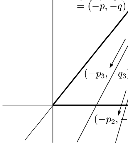
Figure 1: Pictorial rendering of the identity (3.13) for $L=4$

The identity (3.13) can be understood pictorially when $u^{(\ell)}>0$ for $\forall\ell$, as depicted in Figure 1 for $L=4$. In this figure, each points $(m,n)$ corresponds to the factor

$$\log(a_{\alpha\beta}+m\epsilon_{1}^{(0)}+n\epsilon_{2}^{(0)}).$$ (3.19)

Since

$$\epsilon_{1}^{(\ell)}=-q_{\ell}\epsilon_{1}^{(0)}-p_{\ell}\epsilon_{2}^{(0)},\qquad\epsilon_{2}^{(\ell)}=q_{\ell+1}\epsilon_{1}^{(0)}+p_{\ell+1}\epsilon_{2}^{(0)},$$ (3.20)

each of the summand in the left hand in (3.13) adds lattice points between the lines generated by the vectors $(-q_{\ell},-p_{\ell})$ and $(-q_{\ell+1},-p_{\ell+1})$ starting from the points corresponding to $a^{(\ell)}_{\alpha\beta}$ and $a^{(\ell+1)}_{\alpha\beta}$ respectively. The first term in the r.h.s. corresponds to the points in the region $qn\leq pm,\,n\leq-1$ by definition. The remaining term corresponds to the points in the region surrounded by the bold lines in Figure 1. It is remarkable that the boundary of this region consists of the lines $n=0$, $qn=pm$, and the generating vectors of the dual fan, each of which length is proportional to the magnetic fluxes $u_{\alpha\beta}^{(\ell)}\equiv u_{\alpha}^{(\ell)}-u_{\beta}^{(\ell)}$. We also note that the region is naturally divided into $L-1$ regions, which is interpreted as the contribution from each blown-up sphere. From (B.15) and (3.20), we see that the point corresponding to $a^{(\ell)}_{\alpha\beta}$ satisfies the condition

$$(m,n)=(k^{(1)}_{\alpha\beta},0)\,\,{\rm mod}\,\,\mathbb{Z}^{2},$$ (3.21)

which is part of the condition for the summation in (3.11). Moreover, the basis $\epsilon_{1}^{(\ell)}$ and $\epsilon_{2}^{(\ell)}$ generates the lattice points exactly the same as those generated by $\epsilon_{1}^{(0)}$ and $\epsilon_{2}^{(0)}$ because $p_{\ell}q_{\ell+1}-q_{\ell}p_{\ell+1}=1$. Therefore, each term in (3.13) adds the points satisfying the condition (3.21) inside its relative region as previously stated and this explains the identity (3.13).

By using the identity (3.13), we find that the blow-up formula for the one-loop part is given by

$$\prod_{\ell=0}^{L-1}Z_{\rm 1-loop}^{\mathbb{C}^{2}}\left(\epsilon_{1}^{(\ell)},\epsilon_{2}^{(\ell)},\vec{a}^{(\ell)}\right)=\ell_{\rm vector}(\epsilon_{1},\epsilon_{2},\{\vec{k}^{(\ell)}\})Z^{X_{p,q}}_{\rm 1-loop}(\epsilon_{1},\epsilon_{2},\vec{a},p\vec{k}^{(1)}),$$ (3.22)

where

$$\ell_{\rm vector}(\epsilon_{1},\epsilon_{2},\{\vec{k}^{(\ell)}\})=\prod_{\ell=0}^{L-1}\prod_{\alpha\neq\beta}\exp\left(-f_{p,q}^{(\ell)}(a^{(\ell)}_{\alpha\beta},\epsilon_{1}^{(\ell)},\epsilon_{2}^{(\ell)},k^{(\ell)}_{\alpha\beta},k^{(\ell+1)}_{\alpha\beta})\right).$$ (3.23)

3.3 Instanton partition function

The instanton partition function is obtained by combining the full blow-up formula (2.1) with the results in section 3.1 and 3.2. Since the one-loop factor depends on $\vec{k}^{(1)}$ mod $\mathbb{Z}$, the full partition function is written by the sum of these sectors,

$$Z_{\rm full}^{X_{p,q}}(\epsilon_{1},\epsilon_{2},\vec{a},\{\xi_{\ell}\})=Z_{\rm cl}^{X_{p,q}}(\epsilon_{1},\epsilon_{2},\vec{a})\displaystyle\sum_{I_{1}=0}^{p-1}\cdots\sum_{I_{N}=0}^{p-1} Z_{\rm 1-loop}^{X_{p,q}}\left(\epsilon_{1},\epsilon_{2},\vec{a},\vec{I}\right)Z_{\rm inst}^{X_{p,q}}\left(\epsilon_{1},\epsilon_{2},\vec{a},\vec{I},\{\xi_{\ell}\}\right)$$

where $\vec{I}=p\vec{k}^{(1)}$ mod $p$ parametrizes the holonomy class of the gauge field in the Cartan torus. Finally, by using the classical (3.3), the one-loop (3.22), and the full blow-up formula (2.1), we obtain the instanton partition function as

$$Z_{\rm inst}^{X_{p,q}}\left(\epsilon_{1},\epsilon_{2},\vec{a},\vec{I},\{\xi_{\ell}\}\right)= \sum_{{\{\vec{u}_{(\ell)}\}\in\mathbb{Z}^{N(L-1)}}\atop{p\vec{k}^{(1)}=\vec{I}\,\,{\rm mod}\,p}}q^{\frac{1}{2}\sum_{\ell,m}\vec{k}^{(\ell)}\cdot C_{\ell m}\vec{k}^{(m)}}\times\ell_{\rm vector}(\epsilon_{1},\epsilon_{2},\{\vec{k}^{(\ell)}\})$$ (3.25)

$$\qquad\qquad\times\prod_{\ell=0}^{L-1}Z_{\rm inst}^{{\mathbb{C}}^{2}}\left(\epsilon_{1}^{(\ell)},\epsilon_{2}^{(\ell)},\vec{a}^{(\ell)}\right)\times\prod_{\ell=1}^{L-1}\xi_{\ell}^{\sum_{\alpha=1}^{N}u_{\alpha(\ell)}},$$ (3.26)

where $u_{\alpha(\ell)}=C_{\ell m}k_{\alpha}^{(m)}$.

3.4 ALE space

In this subsection we explicitly consider the above formulae for the ALE case, namely $q=p-1$. In this case, $L=p$, and $p_{\ell}=\ell$. The classical partition function is given by (3.1). The one-loop partition function is given as

$$Z^{\rm ALE}_{\rm 1-loop}(\epsilon_{1},\epsilon_{2},\vec{a},\{\vec{k}^{(\ell)}\})= \prod_{\ell=0}^{p-1}\prod_{\alpha\neq\beta}g^{(\ell)}(a^{(\ell)}_{\alpha\beta},\epsilon_{1}^{(\ell)},\epsilon_{2}^{(\ell)},k^{(\ell)}_{\alpha\beta},k^{(\ell+1)}_{\alpha\beta})\prod_{\ell=0}^{p-1}Z_{\rm 1-loop}^{\mathbb{C}^{2}}\left(\epsilon_{1}^{(\ell)},\epsilon_{2}^{(\ell)},\vec{a}^{(\ell)}\right)$$ (3.27)

with

$$g^{(\ell)}(a,e_{1},e_{2},\mu,\nu)\equiv\left\{\begin{array}[]{cll}\displaystyle\prod_{{m\geq 0,n\leq-1}\atop\ell(\nu+m)\leq(\ell+1)(\mu+n)}\left(a+me_{1}+ne_{2}\right)&&\ell\nu<(\ell+1)\mu\\ 1&&\ell\nu=(\ell+1)\mu\\ \\ \displaystyle\prod_{{m\leq-1,n\geq 0}\atop\ell(\nu+m)>(\ell+1)(\mu+n)}\left(a+me_{1}+ne_{2}\right)&&\ell\nu>(\ell+1)\mu\end{array}\right..$$ (3.32)

Here $a_{\alpha}^{(\ell)}$ is defined in (2.2) and $\epsilon_{1}^{(\ell)}$, $\epsilon_{2}^{(\ell)}$ are given in (A.20). Note that the dependence on $\{\vec{k}^{(\ell)}\}$ actually reduces to the dependence on $p\vec{k}^{(1)}$ mod $p$. The instanton partition function is given by

$$Z_{\rm inst}^{\rm ALE}\left(\epsilon_{1},\epsilon_{2},\vec{a},\vec{I},\{\xi_{\ell}\}\right) =\sum_{{\{\vec{u}_{(\ell)}\}\in\mathbb{Z}^{N(p-1)}}\atop{p\vec{k}^{(1)}=\vec{I}\,\,{\rm mod}\,p}}q^{\frac{1}{2}\sum_{\ell,m}\vec{k}^{(\ell)}\cdot C_{\ell m}\vec{k}^{(m)}}\prod_{\ell=0}^{p-1}g^{(\ell)}(a^{(\ell)}_{\alpha\beta},\epsilon_{1}^{(\ell)},\epsilon_{2}^{(\ell)},k^{(\ell)}_{\alpha\beta},k^{(\ell+1)}_{\alpha\beta}){}^{-1}$$ (3.33)

$$\qquad\qquad\times\prod_{\ell=0}^{p-1}Z_{\rm inst}^{{\mathbb{C}}^{2}}\left(\epsilon_{1}^{(\ell)},\epsilon_{2}^{(\ell)},\vec{a}^{(\ell)}\right)\prod_{\ell=1}^{p-1}\xi_{\ell}^{\sum_{\alpha=1}^{N}u_{\alpha(\ell)}}.$$

We note that $C$ is the $A_{p-1}$ Cartan matrix and $\vec{I}$ specifies the twisted sector:

$$\vec{a}\to\vec{a}-\frac{2\pi\vec{I}}{p}.$$ (3.34)

In appendix C we list the explicit first orders of the instanton partition function of $U(2)$ SYM theory on the $A_{2}$ ALE space.

4 M-theory on toric singularities and blow-up formulae

In this section we discuss how the blow-up formulae in the $\epsilon_{1},\epsilon_{2}\to 0$ limit of section 2 can be derived from M-theory considerations. As we will shortly explain, these can be obtained by considering the classical partition function of a single M5-brane on a suitable product geometry. The $\epsilon$-corrections should be calculable from the quantum contribution to the M5-partition function at least in the $\epsilon_{1}+\epsilon_{2}=0$ case via a generalization of [20], but we will not discuss this issue in the present paper.

Let us recall that the low-energy effective theory of $\mathcal{N}=2$ four-dimensional gauge theory is described by a single space-time filling M5-brane wrapping the Seiberg-Witten curve [21], so that the appropriate six-dimensional manifold is the direct product $M_{6}=\Sigma\times X_{p,q}$. We will show that the M5-brane partition function can be computed in this setting. Let us first quickly review the case of compact six-manifolds and then specify the modifications relevant to the non-compact case.

The world-volume theory of the M5-brane is described by an anti-self-dual tensor multiplet $T$ minimally coupled with a three-form gauge field $C_{3}$ by a term $\int_{M_{6}}T\wedge{C}_{3}$. Let us consider a symplectic basis $E_{A}=(e^{a},\tilde{e}_{b})$ for the middle cohomology $H^{3}(M_{6},{\mathbb{Z}})$ of the six-manifold $M_{6}$

$$\int_{M_{6}}E_{A}\wedge E_{B}=J_{AB},$$ (4.1)

namely

$$\int_{M_{6}}e^{a}\wedge e^{b}=0,\ \ \int_{M_{6}}\tilde{e}_{a}\wedge\tilde{e}_{b}=0,\ \ \int_{M_{6}}e^{a}\wedge\tilde{e}_{b}=\delta^{a}_{b},$$ (4.2)

where $J_{AB}=\mbox{1}\mbox{l}\otimes$$\begin{pmatrix}0&1\\ -1&0\end{pmatrix}$. Then the period matrix $Z=Z^{(1)}+iZ^{(2)}$ is defined by expanding

$$\tilde{e}_{a}=Z^{(1)}_{ab}e^{b}+Z^{(2)}_{ab}\star e^{b}.$$ (4.3)

The simplest way to get the M5-brane classical contribution is by computing the full partition function of an abelian two-form potential $T=dB$ in six dimensions. This holomorphically factorizes in chiral times anti-chiral blocks. The M5-brane partition function is extracted as one of such chiral blocks, in the very same way as chiral partition functions are obtained in two-dimensions [22, 23, 24, 25, 26]. The explicit form of this partition function is given in terms of a theta function $\Theta(\overline{Z})$ with suitable characteristics and arguments. The arguments of the theta function are related to the period matrix of the six-manifold and the background value of the $C$-field.

This approach can be extended also to non-compact six-manifolds. In this case, one should restrict to the $L^{2}$ sector of the middle cohomology in order to count finite action configurations only. In particular, let us consider $M_{6}=\Sigma\times X_{p,q}$. In this case, the Künneth decomposition of the middle cohomology reads

$$H^{3}(\Sigma\times X_{p,q},{\mathbb{Z}})=H^{1}(\Sigma,{\mathbb{Z}})\otimes H^{2}(X_{p,q},{\mathbb{Z}}).$$ (4.4)

Let us choose a polarization given by a symplectic basis

$$e^{\alpha(n)} = [b^{\alpha}]\wedge\omega^{n},$$

$$\tilde{e}_{\alpha(m)} = -[a_{\alpha}]\wedge{\cal I}_{m\ell}\omega^{\ell},$$ (4.5)

where $[a_{\alpha}]$ and $[b^{\alpha}]$ are the Poincaré duals of the $a$ and $b$ cycles on $\Sigma$ and ${\cal I}$ satisfies

$${\cal I}_{m\ell}\int_{X_{p,q}}\omega^{\ell}\wedge\omega^{n}=\delta_{m}^{n}\ \ .$$ (4.6)

The $L^{2}$ sector of the middle cohomology of $X_{p,q}$ coincides with the anti-selfdual part of $H^{2}(X_{p,q},{\mathbb{Z}})$ [27]. Therefore, in the subspace which is relevant to our computation, $\star\omega^{m}=-\omega^{m}$ and, by choosing the normalization $\int_{\Delta_{\ell}}\omega^{n}=\delta_{\ell}^{n}$, we get that ${\cal I}=-C$ is nothing but the intersection matrix of $X_{p,q}$ homology cycles, see Appendix A for details. In our notation then $b^{-}\left(X_{p,q}\right)=L-1$.

To compute the period matrix, one can use the standard relation

$$[a_{\alpha}]=-\tau^{(1)}_{\alpha\beta}[b^{\beta}]-\tau^{(2)}_{\alpha\beta}\star[b^{\beta}]$$

which holds on a generic Riemann surface [28], where $\tau=\tau^{(1)}+i\tau^{(2)}$ is its period matrix. Indeed one gets

$$\tilde{e}_{\alpha(m)}=[a_{\alpha}]\wedge C_{mn}\omega^{n}=\left\{-\tau^{(1)}_{\alpha\beta}[b^{\beta}]-\Omega^{(2)}_{\alpha\beta}\star[b^{\beta}]\right\}\wedge C_{mn}\omega^{n}=\left(-\tau^{(1)}_{\alpha\beta}C_{mn}\right)e^{\beta(n)}+\left(\tau^{(2)}_{\alpha\beta}C_{mn}\right)\star e^{\beta(n)}$$

so that the complete period matrix relevant to finite action configurations is

$$Z=-C\otimes\bar{\tau}.$$

Another subtle feature arise in the non-compact case when considering the possible allowed three- form fluxes. Let us show that the most natural condition in M-theory leads to the correct lattice of four-dimensional gauge theory. First of all we expand the three-form $T\in H^{3}(\Sigma\times X_{p,q})$ as

$$T=\hat{k}_{\alpha(m)}e^{\alpha(m)}+\hat{h}^{\alpha(m)}\tilde{e}_{\alpha(m)}$$ (4.7)

and compute its periods on generic compact 3-cycles as

$$\int_{\Gamma^{a}}T=\hat{k}_{\alpha(m)}\int_{\gamma^{i}}[b^{\alpha}]\int_{\Delta_{n}}\omega^{m}-\hat{h}^{\alpha(m)}\int_{\gamma^{i}}[a_{\alpha}]\int_{\Delta_{n}}\omega^{l}C_{lm}=\left\{\begin{array}[]{ll}\hat{k}_{\alpha(m)}(C^{-1})^{mn}&\ \ \mbox{if $i=\alpha$};\\ \hat{h}^{\alpha(m)}&\ \ \mbox{if $i=g+\alpha$}.\end{array}\right.$$ (4.8)

Here $\left\{\Gamma^{a}\right\}=\left\{\Delta_{n}\times\gamma^{i}\right\}$, where $\left\{\gamma^{i}\right\}=\left\{a_{\alpha},b^{\alpha}\right\}$ is our reference basis in $H_{1}(\Sigma,{\mathbb{Z}})$ and $\left\{\Delta_{n}\right\}$ are the blown-up spheres in $X_{p,q}$.

The lattice of the relevant theta function is obtained by dualizing the lattice of the $\{e^{a}\}$ sector [24], namely the first line in the r.h.s. of (4.8). Being this the lattice of fundamental M-theory charges we assume that it is the integer one, namely $\left(C^{-1}\otimes{\bf 1}\right)\hat{k}\in{\mathbb{Z}}^{g(L-1)}$. Then its dual reads $\left(C\otimes{\bf 1}\right)k\in{\mathbb{Z}}^{g(L-1)}$ so that finally

$$k\in(C^{-1}\otimes{\bf 1}){\mathbb{Z}}^{g(L-1)}$$ (4.9)

whose four-dimensional factor describes the magnetic fluxes of the gauge field on $X_{p,q}$. Therefore, the relevant generalized $\Theta$-function contribution is given by the anti-holomorphic block which reads

$$\Theta(C\otimes\tau|Q)=\sum_{k\in(C^{-1}\otimes{\bf 1}){\mathbb{Z}}^{g(L-1)}}e^{\pi i\left[k(C\otimes\tau)k+2Q(C\otimes{\bf 1})k\right]}$$ (4.10)

where $Q$ is a background for the three-form $C$-field which couples to the non-trivial $c_{1}$ of the four-dimensional gauge bundle. Indeed from the minimal coupling term we get

$$\int_{M_{6}}C_{3}\wedge T=\int_{\Sigma\times X_{p,q}}C_{3}\wedge\left(\hat{k}_{\alpha(m)}e^{\alpha(m)}+\hat{h}^{\alpha(m)}\tilde{e}_{\alpha(m)}\right)=\sum_{\alpha(m)}\left(\hat{Q}^{\alpha(m)}\hat{k}_{\alpha(m)}+\tilde{Q}_{\alpha(m)}\hat{h}^{\alpha(m)}\right)$$ (4.11)

where $\hat{Q}^{a}$ and $\tilde{Q}_{a}$ are the components of the background $C$-field. After Poisson resummation, one gets the linear term $kQ$ in (4.10) which reproduces the term $\left(\xi_{m}\right)^{C_{lm}k_{\alpha}^{(m)}}$ in the gauge theory $\theta$-function. The complete background field is actually $Q^{\alpha(m)}=\frac{1}{2\pi i}\ln\xi_{m}+Q^{\alpha(m)}_{grav}$ whose first term describes, after the reduction, the coupling of an external source to the first Chern class of the gauge bundle. The second term $Q_{grav}$ has to be set by considerations of anomaly cancellation conditions. In order to address this issue, one should compute the full quantum mechanical contribution to the partition function in the product geometry. The requirement of modular invariance then would correspond to the anomaly cancellation conditions in the string theory engineering. In general there are pure gravitational and mixed anomalies to cure. Fixing the pure gravitational part means fixing the overall normalization of the M5-brane partition function, namely the coefficients of the $F_{1}$ and $G$ terms in (2.18), while fixing the mixed anomalies corresponds to fix the coefficients of the linear term in the $k_{\alpha}^{(\ell)}$. This corresponds to fix the gravitational part of the background $C$-field as $Q^{\alpha(m)}_{grav}=\partial_{\alpha}H(e_{\ell}-2)$. Although we don’t give an M-theoretic detailed account for this assignment, let us notice that it measures an anomaly induced the lack of the four manifold from being hyperkahler, that is from admitting a reduced holonomy which would make the topologically twisted and the untwisted ${\cal N}=2$ gauge theories equivalent.

It is then easy to recognize that, after the above background value is selected, (4.10) coincides with the ($SU(N)$ part of the) $\vartheta$-function arising in the blow-up formulae of the previous sections (2.18).

5 Two-dimensional CFT counterpart

In this section, we consider the relation between the gauge theories on toric singularities and two-dimensional CFTs. The M-theory argument in the previous section gives a hint to this relation: one side is the four-dimensional gauge theory on $X_{p,q}$ obtained by compactifying M5-branes on a punctured Riemann surface ${\mathcal{C}}$. The other side is the two-dimensional effective theory on ${\mathcal{C}}$ obtained after integration over the four-dimensional modes of the M-theory. As it is well-known, the two-dimensional theory in the case of $\mathbb{R}^{4}_{\epsilon_{1},\epsilon_{2}}$ turns out to be the $W_{N}$ CFT [2, 29] with an extra $U(1)$ free boson factor. The partition function of the gauge theory can be related with the conformal block ${\mathcal{B}}_{W}$ of $W_{N}$-algebra, under a proper identification of the parameters,

$$Z^{\mathbb{C}^{2}}=Z_{{\rm U(1)}}{\mathcal{B}}_{W},$$ (5.1)

where ${\mathcal{B}}_{W}$ is defined in a specific marking of ${\mathcal{C}}$ which in turn corresponds to a particular weak coupling description of the gauge theory. Non-trivial four-dimensional geometry should change the two-dimensional CFT algebra to ${\cal A}_{N}(X_{p,q})$. Indeed, it was found and checked in [30, 10, 18, 31, 19, 32, 33, 34, 35] that the U($N$) gauge theory on the $A_{p-1}$ ALE space is related to the product of the Heisenberg, affine $\hat{su}(p)_{N}$ and $\mathbb{Z}_{p}$ para-$W_{N}$ algebras. In this section, we study this relation by using the gauge theory partition function computed in section 2 and the M-theory considerations presented in section 4, and investigate their possible implications on the mysterious two-dimensional side.

The blowup formula (2.1) directly imply that the fixed points of the moduli space of instantons on $X_{p,q}$ provide a basis for the representation of $L$ copies of Heisenberg plus $W_{N}$ algebrae with suitable central charges related to the $(\epsilon_{1}^{(\ell)},\epsilon_{2}^{(\ell)})$ weights under the $(\mathbb{C}^{*})^{2}$-action

$${\cal A}_{N}(X_{p,q})\equiv\oplus_{\ell=0}^{L-1}(\mathcal{H}\oplus\,^{\ell}W_{N})$$ (5.2)

where the central charge of ${}^{\ell}W_{N}$ is $c_{\ell}=(N-1)\left(1+Q_{\ell}^{2}N(N+1)\right)$, $Q_{\ell}^{2}=\frac{(\epsilon_{1}^{(\ell)})^{2}+(\epsilon_{2}^{(\ell)})^{2}}{\epsilon_{1}^{(\ell)}\epsilon_{2}^{(\ell)}}+2$. As we will see in a moment, the overall central charge of (5.2) coincides with the central charge of the two-dimensional CFT that can be computed from M-theory compactification.

The result (5.2) suggest that in the ALE case $q=p-1$ the conformal blocks of ${\mathbb{Z}}_{p}$ parafermionic $W_{N}$ algebra plus $p$ copies of Heisenberg algebrae can be computed as $p$-nested conformal blocks of the algebra (5.2) in terms of the blowup formula (3.33). This has been shown in [18, 19, 35] in the $p=2$ case, corresponding to the ${\cal N}=1$ super Virasoro algebra whose conformal blocks are known. The conformal blocks for the general case are instead unknown and the blowup formula (3.33) provides a natural candidate for them.

5.1 $U(1)$ partition function and Frenkel-Kac construction

From the mathematical viewpoint, the above correspondence for the ALE case should be viewed as a generalization to higher rank cases of the Frenkel-Kac construction discussed in [36, 37] for Hilbert schemes, i.e. $U(1)$ gauge group. In this subsection, we consider the case of $U(1)$ gauge theory and the relation with the Frenkel-Kac construction more explicitly.

For the abelian case, the instanton partition function (3.33) reduces to

$$Z_{\rm inst}^{\rm ALE}=\sum_{\{u_{(\ell)}\}}q^{\frac{1}{2}\sum_{\ell,m}u_{(\ell)}(C^{-1})^{\ell m}u_{(m)}}\prod_{\ell=0}^{p-1}Z_{\rm inst}^{\mathbb{C}^{2}}(\epsilon^{(\ell)}_{1},\epsilon^{(\ell)}_{2},a^{(\ell)})\prod_{\ell=1}^{p}\xi_{\ell}^{u_{(\ell)}}$$ (5.3)

since $k_{\alpha\beta}=0$, and thus $g^{(\ell)}=1$. This is also the case when we consider ${\cal N}=2^{*}$ theory, where $Z_{\rm inst}^{\mathbb{C}^{2}}$ is replaced by the Nekrasov instanton partition function of the ${\cal N}=2^{*}$ theory on $\mathbb{C}^{2}$. In the ${\cal N}=4$ limit, it further reduces to

$$Z_{\rm inst}^{\rm ALE}=\eta(\tau)^{-p}\sum_{\{u_{(\ell)}\}}q^{\frac{1}{2}\sum_{\ell,m}u_{(\ell)}(C^{-1})^{\ell m}u_{(m)}}\prod_{\ell=1}^{p}\xi_{\ell}^{u_{(\ell)}}.$$ (5.4)

which can also be written as

$$Z_{\rm inst}^{\rm ALE}=\eta^{-1}(\tau)\sum_{\Lambda}\chi_{\Lambda}(\tau,\xi),$$ (5.5)

where $\chi_{\Lambda}$ is the character of the representations $\Lambda$ of the affine $\hat{su}(p)_{1}$ algebra, as found in [38].

On one hand, one can see that (5.3) or (5.4) are related to the direct sum of $p$ copies of the Heisenberg algebra in the two-dimensional CFT side. On the other hand, (5.5) denotes the relation with the algebra $\mathcal{H}\oplus\hat{su}(p)_{1}$ as in [35]. These two different sets of algebras in the two-dimensional CFT side can be understood as the Frenkel-Kac construction [36]: actually, by this construction, $\hat{su}(p)_{1}$ is expressed as the Heisenberg algebra of the type $A_{p-1}$:

$$[a_{i(\ell)},a_{j(m)}]=\delta_{i+j,0}C_{\ell m},$$ (5.6)

where $C_{\ell m}$ is the Cartan matrix for $A_{p-1}$. The corresponding CFT is the theory of free bosons, whose Hamiltonian is given by

$$H=\sum_{\ell,m}\left(\frac{1}{2}a_{0(\ell)}(C^{-1})^{\ell m}a_{0(m)}+\sum_{i=1}^{\infty}a_{-i(\ell)}(C^{-1})^{\ell m}a_{i(m)}\right).$$ (5.7)

From the viewpoint of M-theory, the two-dimensional CFT is obtained by reducing the theory of self dual three-form on $T^{2}\times\mathbb{C}^{2}/Z_{p}$ onto $T^{2}$. Therefore, the target space of the two-dimensional CFT is expected to be the integrable second cohomology of the ALE space modulo integral elements and thus, the momentum lattice is given by that of $A_{p-1}$. The partition function on a torus with the insertion of the fugacity $z_{(\ell)}$ for this theory, which corresponds to the ${\cal N}=4$ theory in the gauge theory side, is given by

$${\rm Tr}\langle q^{H}e^{\sum_{\ell}(C^{-1}z)^{(\ell)}a_{0(\ell)}}\rangle=\eta(\tau)^{-p+1}\sum_{\{u_{(\ell)}\}}q^{\frac{1}{2}\sum_{\ell,m}u_{(\ell)}(C^{-1})^{\ell m}u_{(m)}}\prod_{\ell=1}^{p-1}\xi_{(\ell)}^{u_{(\ell)}},$$ (5.8)

where the integers $u_{(\ell)}$ corresponds to the momenta. By multiplying by the partition function $\eta^{-1}(\tau)$ of one more free boson, which corresponds to the overall $U(1)$ factor in the gauge theory side, it exactly reproduces (5.4).

We expect that the factorization property in (5.8) holds even when we add one-point insertion with finite conformal dimension. In this case, $\eta^{-1}$ function is replaced by the one-point function of the free boson on torus, which is known to coincide with the Nekrasov partition function of the abelian ${\cal N}=2^{*}$ theory on $\mathbb{C}^{2}$ [39], which is consistent with (5.3).

The derivation of the $U(1)$ instanton partition function easily generalizes to non-hyperkahler $\Gamma_{p,q}\subset U(2)$ quotients. The resulting partition function should correspond to the sum of characters of a conjectural chiral algebra defined by the intersection matrix. This however cannot be interpreted in terms of Kac-Moody algebrae since McKay correspondence does not apply.

5.2 Central charges

Let us compute the central charge of the corresponding two-dimensional CFT from the anomaly polynomial of the six-dimensional (2,0) theory [8, 9, 10]. Consider $N$ M5-branes compactified on a four-manifold $X$. Under a suitable twist, the integrated anomaly eight-form over $X$ leads to the central charge of the remaining two-dimensional theory:

$$c=N\chi(X)+N(N^{2}-1)(P_{1}(X)+2\chi(X)).$$ (5.9)

where $\chi(X)=\int_{X}e(X)$ and $P_{1}(X)=\int_{X}p_{1}(X)$ are the equivariant Euler number and the integrated first Pontryagin class respectively.

Let us focus on $X=X_{p,q}$, namely the blow up of a toric singularity $\mathbb{C}^{2}/\Gamma_{p,q}$. Since we are working with the deformation $\epsilon_{1,2}$, $\chi(X_{p,q})$ and $P_{1}(X_{p,q})$ should be computed in the equivariant sense. This gives the following results

$$\chi(X_{p,q})=\sum_{\ell=0}^{L-1}1=L,~{}~{}~{}~{}P_{1}(X_{p,q})=\sum_{\ell=0}^{L-1}\frac{(\epsilon_{1}^{(\ell)})^{2}+(\epsilon_{2}^{(\ell)})^{2}}{\epsilon_{1}^{(\ell)}\epsilon_{2}^{(\ell)}},$$ (5.10)

where $L$ is the number of the fixed points of the torus action and $\epsilon_{1,2}^{(\ell)}$ are given in (A.20). By plugging these values into (5.9) we recover the central charge of the algebra (5.2). The central charge can be easily expressed through $N_{G}$ defined in (2.19) as

$$c=NL+N(N^{2}-1)\left(\frac{Q^{2}}{p}-N_{G}\right).$$ (5.11)

Note that since $\epsilon_{1}$ and $\epsilon_{2}$ enter symmetrically in the above formula, also the coefficient $N_{G}$ is also symmetric under the exchange $q\leftrightarrow q_{L-1}$, following from the argument just below (2.11).

$A_{p-1}$ ALE space

In the case of the blow up of $\mathbb{C}^{2}/\mathbb{Z}_{p}$ ($q=p-1$), the number of the fixed points is $p$ and the $\epsilon_{1,2}^{(\ell)}$ are given in (A.9). Thus, we get

$$c=Np+\frac{N(N^{2}-1)Q^{2}}{p},$$ (5.12)

where we defined $Q=b+1/b$ with $\sqrt{\epsilon_{1}/\epsilon_{2}}=b$. One can check that this is indeed the sum of the central charges of the Heisenberg, affine $\hat{su}(p)_{N}$ and $p$-th para-$W_{N}$ algebras, as found in [10]:

$$c=1+\frac{N(p^{2}-1)}{N+p}+\left(\frac{p(N^{2}-1)}{N+p}+\frac{N(N^{2}-1)Q^{2}}{p}\right).$$ (5.13)

${\mathcal{O}}_{\mathbb{P}^{1}}(-p)$ space

In the case of the ${\mathcal{O}}_{\mathbb{P}^{1}}(-p)$ space ($q=1$), the number of the fixed points is $2$ and the $\epsilon_{1,2}^{(\ell)}$ are given in (A.6). Therefore, we obtain

$$c=2N+\frac{N(N^{2}-1)}{p}\left(Q^{2}-(p-2)^{2}\right).$$ (5.14)

In the case of $p=2$, this coincides with (5.12) with $p=2$.

Other examples

For example, we can compute the first cases which are not of the two types above. For $\Gamma_{5,2}$ and $\Gamma_{5,3}$, we get, due to the $q\leftrightarrow p_{L-1}$ symmetry, the same result

$$c=3N+\frac{N(N^{2}-1)}{5}\left(Q^{2}-2\right).$$ (5.15)

For $\Gamma_{7,2}$, we get

$$c=3N+\frac{N(N^{2}-1)}{7}\left(Q^{2}-8\right).$$ (5.16)

6 Conclusions and open issues

In this paper we started a systematic study of ${\cal N}=2$ gauge theories on toric singularities. The results we obtained raise a number of issues that it would be interesting to further study.

First of all, the blow-up formula (2.1) together with AGT correspondence implies that the instanton partition function provides an analytic form for the conformal blocks of the algebra ${\cal A}_{N}(X_{p,q})$ we discussed in section 5, see (5.2). Moreover, the one-loop contribution should be interpreted as the three-point functions of the corresponding two-dimensional CFT. These should be regarded as the structure constants of the OPE algebra of primaries, whose spectrum is not known at the moment for general $X_{p,q}$ varieties. It would be interesting to investigate further this issue. In the ALE case a natural candidate has been proposed in [10] as the ${\mathbb{Z}}_{p}$ parafermionic $W_{N}$ theory, whose conformal blocks and three-point functions are however not known in general. Our result can be regarded as a proposal for their computation. Let us remark that for $p=N=2$ this is verified both for the conformal blocks [30, 18, 33, 35] and the three-point functions [19] and for $p=4$, $N=2$ case in [32, 34]. In the ALE case and $N=2$ one might compare our one-loop formulas with the parafermionic Liouville three-point functions as given in [40].

Another interesting aspect that could help in elucidating the above problem is to investigate the ${\cal N}=4$ limit of the partition function in the generic $\Gamma_{p,q}$ case, which should be expressed in terms of the characters of the full conformal algebra [19]. It could be useful in this respect to study the level-rank duality properties of these partition functions in full generality. Let us remark that the algebraic structure that we find in the ALE case contains as a factor the Kac-Moody algebrae found in [41] and further discussed in [42, 43, 44, 45].

Although we did not discuss two-dimensional CFT correlators, we expect that these would arise by computing the ${\cal N}=2$ partition function on $S^{4}/\Gamma_{p,q}$ along the lines of [46]. It would be also interesting to study BPS observables in the gauge theory on toric singularities, in particular surface operators and their possible relationship with degenerate fields insertions in the two-dimensional CFT.

The results presented in this paper are obtained under some natural quantum field theoretic assumptions, namely the patch-by-patch factorization of the full partition function. This is a well established result for some particular cases, and it would be relevant to have a rigorous proof in general. This would amount to have a direct computation of the $\ell$-factor in (3.23) from the localization formula in each topological sector of the theory. To this end a generalization of the ADHM of [47] to $\Gamma_{p,q}$ orbifolds would also be welcome. This could also help to extend the rigorous proof of the AGT correspondence of [48] to instanton counting on toric singularities.

An open problem is the geometric engineering of these four-dimensional gauge theories, which would shed light on the topological string description of their Nekrasov partition function at least in the unrefined $\epsilon_{1}+\epsilon_{2}=0$ case. This issue would naturally lead to a comparison with the results of [49] where the holomorphic anomaly equation for the $A_{1}$ ALE space is discussed.

Finally, the rôle of integrable systems in this whole story has to be elucidated. Our result (2.1) again suggests the emergence of a quiver integrable system made of nested copies of the systems relevant for the flat space, whose intertwining is dictated by the intersection matrix of the $X_{p,q}$ variety. For example for linear quivers we expect to obtain nested copies of the Calogero-Sutherland system, which is the relevant one in the flat space case [50, 48]. A more general view on the problem would be gained in terms of a suitable generalization of the Hitchin system approach to $X_{p,q}$ varieties.

Appendix

Appendix A Hirzebruch-Jung resolution:

The $(p,q)$ toric singularity is the quotient ${\mathbb{C}}^{2}/\Gamma_{p,q}$, where the action is in local coordinates $z_{1}\to e^{2\pi i/p}z_{1}$ and $z_{2}\to e^{2\pi iq/p}z_{2}$, with $(p,q)$ being coprime and $q<p$.

The Hirzebruch-Jung resolution of the above singularity is prescribed as follows. Let $p/q=[e_{1},\ldots,e_{L-1}]\equiv e_{1}-\frac{1}{e_{2}-\frac{1}{e_{3}-\ldots}}$ be the continuous fraction expansion of the ratio $p/q$ in terms of the finite sequence of positive integers $\{e_{1},\ldots,e_{L-1}\}$. The fan of the resolved toric variety is given in terms of the set of vectors $\left\{v_{\ell}\right\}_{\ell=0,\ldots,L}$ in ${\mathbb{Z}}^{2}$ satisfying the recursion relation $v_{\ell+1}+v_{\ell-1}=e_{\ell}v_{\ell}$ with boundary conditions $v_{0}=(0,1)$ and $v_{L}=(p,-q)$. Each internal vector $v_{\ell}$, $\ell=1,\ldots,L-1$ of the fan corresponds to a blown-up sphere $\Delta_{\ell}$. Recalling that the intersection pairing of these spheres can be computed from the toric fan as $\Delta_{\ell}\cdot\Delta_{\ell}=v_{\ell-1}\wedge v_{\ell+1}$ and $\Delta_{\ell}\cdot\Delta_{\ell+1}=v_{\ell}\wedge v_{\ell+1}$, we can compute the intersection matrix to be

$${\cal I}_{p,q}\equiv-C=\begin{pmatrix}-e_{1}&1&0&\dots&0\\ 1&-e_{2}&\ddots&{}&{}\\ 0&\ddots&\ddots&\ddots&{}\\ \vdots&{}&\ddots&\ddots&1\\ 0&{}&{}&1&-e_{L-1}\end{pmatrix}$$ (A.1)

The cones of the fan are $\sigma_{\ell}=\{v_{\ell},v_{\ell+1}\}$, with $\ell=0,\ldots,L-1$, and those of the the dual fan $\sigma_{\ell}^{\star}=\{-v_{\ell}\tau_{2},v_{\ell+1}\tau_{2}\}$, where $\tau_{2}=$$\begin{pmatrix}0&1\\ -1&0\end{pmatrix}$. The ring of holomorphic functions on the toric variety can be described in terms of the dual cones as follows. Let us denote the entries of the vectors of the dual fan as $\sigma_{\ell}^{\star}=\left\{(s_{\ell},t_{\ell}),(\tilde{s}_{\ell},\tilde{t}_{\ell})\right\}$. By using this notation, the polynomial ring reads

$$\oplus_{\ell=0}^{L-1}{\mathbb{C}}[w_{1}^{s_{\ell}}w_{2}^{t_{\ell}},w_{1}^{\tilde{s}_{\ell}}w_{2}^{\tilde{t}_{\ell}}]=\oplus_{\ell=0}^{L-1}{\mathbb{C}}[z_{1}^{ps_{\ell}-qt_{\ell}}z_{2}^{t_{\ell}},z_{1}^{p\tilde{s}_{\ell}-q\tilde{t}_{\ell}}z_{2}^{\tilde{t}_{\ell}}],$$ (A.2)

where we used the invariant variables $w_{1}=z_{1}^{p}$ and $w_{2}=z_{2}/z_{1}^{q}$.

The torus action $({\mathbb{C}}^{\ast})^{2}$ on the singular variety $(z_{1},z_{2})\to(e^{i\epsilon_{1}}z_{1},e^{i\epsilon_{2}}z_{2})$ descends to a torus action on the resolved variety whose weights can be obtained directly from (A.2) as

$$\epsilon_{1}^{(\ell)} = (ps_{\ell}-qt_{\ell})\epsilon_{1}+t_{\ell}\epsilon_{2},$$

$$\epsilon_{2}^{(\ell)} = (p\tilde{s}_{\ell}-q\tilde{t}_{\ell})\epsilon_{1}+\tilde{t}_{\ell}\epsilon_{2}.$$ (A.3)

Let us now consider some explicit examples that are relevant for the main text calculations.

A.1 $\mathcal{O}_{\mathbb{P}^{1}}(-p)$ space

The resolution of the $\Gamma_{p,1}$ singularity is given by the total space of $\mathcal{O}_{\mathbb{P}^{1}}(-p)$-bundle. The cones are

$$\sigma_{0}=\{(0,1),(1,0)\},\quad\ \ \sigma_{1}=\{(1,0),(p,-1)\},$$ (A.4)

and the dual cones

$$\sigma_{0}^{\star}=\{(1,0),(0,1)\},\quad\ \ \sigma_{1}^{\star}=\{(0,-1),(1,p)\}.$$ (A.5)

The weights of the torus action in the two patches are

$$\epsilon^{(0)}_{1} = p\epsilon_{1},\quad\epsilon^{(0)}_{2}=\epsilon_{2}-\epsilon_{1},$$

$$\epsilon^{(1)}_{1} = \epsilon_{1}-\epsilon_{2},\quad\epsilon^{(1)}_{2}=p\epsilon_{2}.$$ (A.6)

A.2 $A_{p-1}$ ALE space

The cones of the resolution of the $\Gamma_{p,p-1}$ singularity are

$$\sigma_{\ell}=\{(\ell,1-\ell),(\ell+1,-\ell)\}$$ (A.7)

with $\ell=0,\ldots,p-1$. The dual cones are

$$\sigma_{\ell}^{\star}=\{(1-\ell,-\ell),(\ell,\ell+1)\}.$$ (A.8)

The weights of the torus action in the $p$ patches are

$$\epsilon^{(\ell)}_{1}=(p-\ell)\epsilon_{1}-\ell\epsilon_{2},\quad\epsilon^{(\ell)}_{2}=(-p+\ell+1)\epsilon_{1}+(\ell+1)\epsilon_{2}.$$ (A.9)

A.3 $\Gamma_{5,2}$, $\Gamma_{5,3}$ and $\Gamma_{7,2}$ singularities

Let us consider other simple cases. For the $\Gamma_{5,2}$ case, the cones are

$$\sigma_{0}=\{(0,1),(1,0)\},\quad\ \ \sigma_{1}=\{(1,0),(3,-1)\},\quad\ \ \sigma_{2}=\{(3,-1),(5,-2)\},$$ (A.10)

and the dual cones

$$\sigma_{0}^{\star}=\{(1,0),(0,1)\},\quad\ \ \sigma_{1}^{\star}=\{(0,-1),(1,3)\},\quad\ \ \sigma_{2}^{\star}=\{(-1,-3),(2,5)\}.$$ (A.11)

The weights of the torus action in the three patches are

$$\epsilon^{(0)}_{1} = 5\epsilon_{1},\quad\epsilon^{(0)}_{2}=\epsilon_{2}-2\epsilon_{1},$$

$$\epsilon^{(1)}_{1} = 2\epsilon_{1}-\epsilon_{2},\quad\epsilon^{(1)}_{2}=-\epsilon_{1}+3\epsilon_{2},$$

$$\epsilon^{(2)}_{1} = \epsilon_{1}-3\epsilon_{2},\quad\epsilon^{(2)}_{2}=5\epsilon_{2}.$$ (A.12)

For the $\Gamma_{5,3}$ case, the weights of the torus action in the three patches are

$$\epsilon^{(0)}_{1} = 5\epsilon_{1},\quad\epsilon^{(0)}_{2}=\epsilon_{2}-3\epsilon_{1},$$

$$\epsilon^{(1)}_{1} = 3\epsilon_{1}-\epsilon_{2},\quad\epsilon^{(1)}_{2}=-\epsilon_{1}+2\epsilon_{2},$$

$$\epsilon^{(2)}_{1} = \epsilon_{1}-2\epsilon_{2},\quad\epsilon^{(2)}_{2}=5\epsilon_{2}.$$ (A.13)

Finally, for the $\Gamma_{7,2}$ case, we get the weights of the torus action again in the three patches:

$$\epsilon^{(0)}_{1} = 7\epsilon_{1},\quad\epsilon^{(0)}_{2}=\epsilon_{2}-2\epsilon_{1},$$

$$\epsilon^{(1)}_{1} = 2\epsilon_{1}-\epsilon_{2},\quad\epsilon^{(1)}_{2}=-\epsilon_{1}+4\epsilon_{2},$$

$$\epsilon^{(2)}_{1} = \epsilon_{1}-4\epsilon_{2},\quad\epsilon^{(2)}_{2}=7\epsilon_{2}.$$ (A.14)

A.4 Comment

In this section, we show a way to solve the relation $v_{\ell+1}+v_{\ell-1}=e_{\ell}v_{\ell}$ explicitly. We define the following two sets of sequences of integers:

$$p_{0}=0,\qquad p_{1}=1,\qquad(p_{2}=e_{1}),\qquad p_{\ell+1}=e_{\ell}p_{\ell}-p_{\ell-1}\quad(\ell\geq 1),$$ (A.15)

$$q_{0}=-1,\qquad q_{1}=0,\qquad(q_{2}=1),\qquad q_{\ell+1}=e_{\ell}q_{\ell}-q_{\ell-1}\quad(\ell\geq 1).$$ (A.16)

By definition, they satisfy the same recursion relation as $v_{\ell}$. It is known that $p_{\ell}$ and $q_{\ell}$ are coprime to each other and that they are the numerator and the denominator of $[e_{1},\cdots,e_{\ell-1}]$ respectively:

$$[e_{1},\cdots,e_{\ell-1}]=\frac{p_{\ell}}{q_{\ell}}.\qquad(\ell\geq 2)$$ (A.17)

In particular, this means that $p_{L}=p$ and $q_{L}=q$. It is also known that

$$p_{\ell}q_{\ell+1}-q_{\ell}p_{\ell+1}=1.$$ (A.18)

Comparing the recursion relation and the boundary condition, we identify

$$s_{\ell}=-q_{\ell},\quad\tilde{s}_{\ell}=q_{\ell+1},\quad t_{\ell}=-p_{\ell},\quad\tilde{t}_{\ell}=p_{\ell+1}.$$ (A.19)

In terms of (A.19) we have

$$\epsilon_{1}^{(\ell)} = -(pq_{\ell}-qp_{\ell})\epsilon_{1}-p_{\ell}\epsilon_{2},$$

$$\epsilon_{2}^{(\ell)} = (pq_{\ell+1}-qp_{\ell+1})\epsilon_{1}+p_{\ell+1}\epsilon_{2}.$$ (A.20)

Explicitly,

$$\epsilon_{1}^{(0)}=p\epsilon_{1}, \quad\epsilon_{2}^{(0)}=-q\epsilon_{1}+\epsilon_{2},$$

$$\epsilon_{1}^{(1)}=q\epsilon_{1}-\epsilon_{2}, \quad\epsilon_{2}^{(1)}=(p-qe_{1})\epsilon_{1}+e_{1}\epsilon_{2},$$

$$\epsilon_{1}^{(2)}=(-p+qe_{1})\epsilon_{1}-e_{1}\epsilon_{2}, \quad\epsilon_{2}^{(2)}=\cdots,$$

$$\cdots$$

$$\epsilon_{1}^{(L-2)}=\cdots \quad\epsilon_{2}^{(L-2)}=-\epsilon_{1}+p_{L-1}\epsilon_{2},$$

$$\epsilon_{1}^{(L-1)}=\epsilon_{1}-p_{L-1}\epsilon_{2} \quad\epsilon_{2}^{(L-1)}=p\epsilon_{2},$$ (A.21)

where we have used (A.18) for $\ell=L-1$ to calculate $\epsilon_{2}^{(L-2)}$ and $\epsilon_{1}^{(L-1)}$.

Appendix B Various summations of Omega deformation parameters

By construction, the Omega deformation parameters $\epsilon_{1}^{(\ell)}$ and $\epsilon_{2}^{(\ell)}$ are related by $\epsilon_{1}^{(\ell)}=-\epsilon_{2}^{(\ell-1)}$, and respectively satisfy the recursion relations

$$\epsilon_{1}^{(\ell-1)}+\epsilon_{1}^{(\ell+1)}=e_{\ell}\epsilon_{1}^{(\ell)},\qquad\epsilon_{2}^{(\ell-1)}+\epsilon_{2}^{(\ell+1)}=e_{\ell+1}\epsilon_{2}^{(\ell)}.$$ (B.1)

They satisfy the boundary condition $\epsilon_{1}^{(0)}=p\epsilon_{1}$ and $\epsilon_{2}^{(L-1)}=p\epsilon_{2}$.

It follows from (A.18) that

$$p_{\ell+1}\epsilon_{1}^{(\ell)}+p_{\ell}\epsilon_{2}^{(\ell)}=\epsilon_{1}^{(0)}.$$ (B.2)

By using this identity and (A.20), we can show that

$$\sum_{\ell=0}^{m}\frac{1}{\epsilon_{1}^{(\ell)}\epsilon_{2}^{(\ell)}}=\frac{p_{m}}{\epsilon_{1}^{(0)}\epsilon_{2}^{(m)}},$$ (B.3)

which for $m=L-1$ is

$$\sum_{\ell=0}^{L-1}\frac{1}{\epsilon_{1}^{(\ell)}\epsilon_{2}^{(\ell)}}=\frac{p}{\epsilon_{1}^{(0)}\epsilon_{2}^{(L-1)}}=\frac{1}{p\epsilon_{1}\epsilon_{2}}.$$ (B.4)

We list here other useful formulae used in section 2:

$$\sum_{\ell=0}^{L-1}\frac{\epsilon_{1}^{(\ell)}+\epsilon_{2}^{(\ell)}}{\epsilon_{1}^{(\ell)}\epsilon_{2}^{(\ell)}} = \frac{\epsilon_{1}+\epsilon_{2}}{p\epsilon_{1}\epsilon_{2}},$$ (B.5)

$$\sum_{\ell=0}^{L-1}\frac{\epsilon_{1}^{(\ell)}k^{(\ell+1)}_{\alpha}+\epsilon_{2}^{(\ell)}k^{(\ell)}_{\alpha}}{\epsilon_{1}^{(\ell)}\epsilon_{2}^{(\ell)}} = 0,$$ (B.6)

$$\sum_{\ell=0}^{L-1}\frac{(\epsilon_{1}^{(\ell)}+\epsilon_{2}^{(\ell)})^{2}}{\epsilon_{1}^{(\ell)}\epsilon_{2}^{(\ell)}} = \frac{(\epsilon_{1}+\epsilon_{2})^{2}}{p\epsilon_{1}\epsilon_{2}}-\frac{p_{L-1}+q+2}{p}+2L-\sum_{\ell=1}^{L-1}e_{\ell},$$ (B.7)

$$\Bigl{(} = \frac{(\epsilon_{1}+\epsilon_{2})^{2}}{p\epsilon_{1}\epsilon_{2}}+\frac{2p-2-p_{L-1}-q}{p}+\sum_{\ell=1}^{L-1}(2-e_{\ell})\Bigr{)}$$

$$\sum_{\ell=0}^{L-1}\frac{(\epsilon_{1}^{(\ell)}+\epsilon_{2}^{(\ell)})(\epsilon_{1}^{(\ell)}k^{(\ell+1)}_{\alpha}+\epsilon_{2}^{(\ell)}k^{(\ell)}_{\alpha})}{\epsilon_{1}^{(\ell)}\epsilon_{2}^{(\ell)}} = \sum_{\ell=1}^{L-1}(2-e_{\ell})k_{\alpha}^{(\ell)},$$ (B.8)

$$\Bigl{(} = k^{(1)}_{\alpha}+k^{(L-1)}_{\alpha}-\sum_{\ell=1}^{L-1}\sum_{m=1}^{L-1}C_{\ell m}k^{(m)}_{\alpha}\Bigr{)}$$

$$\sum_{\ell=0}^{L-1}\frac{(\epsilon_{1}^{(\ell)}k^{(\ell+1)}_{\alpha}+\epsilon_{2}^{(\ell)}k^{(\ell)}_{\alpha})(\epsilon_{1}^{(\ell)}k^{(\ell+1)}_{\beta}+\epsilon_{2}^{(\ell)}k^{(\ell)}_{\beta})}{\epsilon_{1}^{(\ell)}\epsilon_{2}^{(\ell)}} = -\sum_{\ell=1}^{p-1}\sum_{m=1}^{p-1}k^{(\ell)}_{\alpha}C_{\ell m}k^{(m)}_{\beta},$$ (B.9)

Note that (B.7) respect the symmetry exchanging

$$p_{L-1}=\frac{p}{[e_{L-1},\cdots,e_{1}]}\quad{\rm and}\quad q=\frac{p}{[e_{1},\cdots,e_{L-1}]}.$$ (B.10)

Derivation of (2.2) from (2.11)

From (2.11) we have

$$a^{(\ell)}_{\alpha} = a_{\alpha}-\sum_{\ell=1}^{L-1}(pq_{\ell}-qp_{\ell})u_{(\ell)\alpha}\epsilon_{1}-\sum_{m=1}^{\ell}u_{(m)\alpha}\epsilon_{1}^{(m)}=a_{\alpha}-\sum_{m=0}^{\ell}u_{(m)\alpha}\epsilon_{1}^{(m)},$$ (B.11)

where we have defined

$$u_{(0)\alpha}\equiv\sum_{\ell=1}^{L-1}\frac{pq_{\ell}-qp_{\ell}}{p}u_{(\ell)\alpha}.$$ (B.12)

Now, we are going to rewrite it in terms of $k=C^{-1}u$. Note that

$$pq_{\ell}-qp_{\ell}=-p\left(C^{-1}\right)^{1\ell}$$ (B.13)

for $1\leq\ell\leq L-1$. Therefore, (B.12) is rewritten as

$$u_{(0)\alpha}=\sum_{\ell=1}^{L-1}\frac{pq_{\ell}-qp_{\ell}}{p}u_{(\ell)\alpha}=-\sum_{\ell=1}^{L-1}\left(C^{-1}\right)^{1\ell}u_{(\ell)\alpha}=-k^{(1)}_{\alpha}$$ (B.14)

and thus, (B.11) is rewritten as

$$a^{(\ell)}_{\alpha}=a_{\alpha}+k^{(1)}_{\alpha}\epsilon_{1}^{(0)}-\sum_{m=1}^{\ell}u_{(m)\alpha}\epsilon_{1}^{(m)}.$$ (B.15)

By considering the third term and taking into account that $k^{(0)}=k^{(L)}=0$, we find

$$-\sum_{m=1}^{\ell}u_{(m)\alpha}\epsilon_{1}^{(m)}=-k^{(1)}_{\alpha}\epsilon_{1}^{(0)}+k^{(\ell+1)}_{\alpha}\epsilon_{1}^{(\ell)}+k^{(\ell)}_{\alpha}\epsilon_{2}^{(\ell)},$$ (B.16)

where we used (B.1). Therefore, we finally obtain the shift formula (2.2).

Appendix C $U(2)$ SYM theory on $A_{2}$ ALE

We give the explicit calculation for the $A_{2}$ ALE instanton partition function. We expand the instanton partition function (3.33) as

$$Z_{\rm inst}(\epsilon_{1},\epsilon_{2},a;\vec{I};c_{1}^{(1)},c_{1}^{(2)})=\sum_{c^{(1)},~{}c^{(2)}}Z^{(c^{(1)},~{}c^{(2)})}(\vec{I})\xi_{1}^{c_{1}^{(1)}}\xi_{2}^{c_{1}^{(2)}},$$ (C.1)

where $a\equiv(a_{1}-a_{2})/2$ and $I_{\alpha}=3k_{\alpha}^{(1)}$ mod $3$. We note that $\vec{k}^{(1)}$ and $c_{1}^{(\ell)}$ are not independent but are related as

$$c_{1}^{(1)}-c_{1}^{(2)}=-(I_{1}+I_{2})\qquad{\rm mod}\,\,3.$$ (C.2)

We calculate the lowest order in instanton number for $-1\leq c_{1}^{(1)},c_{1}^{(2)}\leq 1$. The results are given by

$$Z^{(0,0)}(0,0)=1+\cdots$$

$$Z^{(0,0)}(1,2)$$ (C.3)

$$=\left[\frac{-1}{(2a-\epsilon_{2})(2a+\epsilon_{1})}+\frac{-1}{(2a+\epsilon_{1})(2a+2\epsilon_{1}+\epsilon_{2})}+\frac{-1}{(2a-\epsilon_{1}-2\epsilon_{2})(2a-\epsilon_{2})}\right]q^{\frac{2}{3}}+\cdots$$

$$Z^{(0,0)}(2,1)$$ (C.4)

$$=\left[\frac{-1}{(2a+\epsilon_{2})(2a-\epsilon_{1})}+\frac{-1}{(2a-\epsilon_{1})(2a-2\epsilon_{1}-\epsilon_{2})}+\frac{-1}{(2a+\epsilon_{1}+2\epsilon_{2})(2a+\epsilon_{2})}\right]q^{\frac{2}{3}}+\cdots$$

$$Z^{(0,1)}(2,2)=\left[\frac{-1}{(2a-\epsilon_{1}-\epsilon_{2})(2a)}+\frac{-1}{(2a)(2a+\epsilon_{1}+\epsilon_{2})}\right]q^{\frac{2}{3}}+\cdots$$

$$Z^{(0,1)}(0,1)=q^{\frac{1}{3}}+\cdots$$

$$Z^{(0,1)}(1,0)=q^{\frac{1}{3}}+\cdots$$

$$Z^{(1,0)}(1,1)=\left[\frac{-1}{(2a-\epsilon_{1}-\epsilon_{2})(2a)}+\frac{-1}{(2a)(2a+\epsilon_{1}+\epsilon_{2})}\right]q^{\frac{2}{3}}+\cdots$$

$$Z^{(1,0)}(0,2)=q^{\frac{1}{3}}+\cdots$$

$$Z^{(1,0)}(2,0)=q^{\frac{1}{3}}+\cdots$$

$$Z^{(0,-1)}(1,1)=\left[\frac{-1}{(2a-\epsilon_{1}-\epsilon_{2})(2a)}+\frac{-1}{(2a)(2a+\epsilon_{1}+\epsilon_{2})}\right]q^{\frac{2}{3}}+\cdots$$

$$Z^{(0,-1)}(0,2)=q^{\frac{1}{3}}+\cdots$$

$$Z^{(0,-1)}(2,0)=q^{\frac{1}{3}}+\cdots$$

$$Z^{(-1,0)}(2,2)=\left[\frac{-1}{(2a-\epsilon_{1}-\epsilon_{2})(2a)}+\frac{-1}{(2a)(2a+\epsilon_{1}+\epsilon_{2})}\right]q^{\frac{2}{3}}+\cdots$$

$$Z^{(-1,0)}(0,1)=q^{\frac{1}{3}}+\cdots$$

$$Z^{(-1,0)}(1,0)=q^{\frac{1}{3}}+\cdots$$

$$Z^{(1,1)}(0,0)=\left[\frac{-1}{(2a-\epsilon_{1}-\epsilon_{2})(2a)}+\frac{-1}{(2a)(2a+\epsilon_{1}+\epsilon_{2})}\right]q^{\frac{2}{3}}$$

$$Z^{(1,1)}(1,2)=q+\cdots$$

$$Z^{(1,1)}(2,1)=q+\cdots$$

$$Z^{(-1,-1)}(0,0)=\left[\frac{-1}{(2a-\epsilon_{1}-\epsilon_{2})(2a)}+\frac{-1}{(2a)(2a+\epsilon_{1}+\epsilon_{2})}\right]q+\cdots$$

$$Z^{(-1,-1)}(1,2)=q^{\frac{2}{3}}+\cdots$$

$$Z^{(-1,-1)}(2,1)=q^{\frac{2}{3}}+\cdots$$

$$Z^{(1,-1)}(2,2)=\left[\frac{-1}{(2a-\epsilon_{1}-\epsilon_{2})(2a)}+\frac{-1}{(2a)(2a+\epsilon_{1}+\epsilon_{2})}\right]q^{\frac{2}{3}}+\cdots$$

$$Z^{(1,-1)}(0,1)=q^{\frac{1}{3}}+\cdots$$

$$Z^{(1,-1)}(1,0)=q^{\frac{1}{3}}+\cdots$$

$$Z^{(-1,1)}(1,1)=\left[\frac{-1}{(2a-\epsilon_{1}-\epsilon_{2})(2a)}+\frac{-1}{(2a)(2a+\epsilon_{1}+\epsilon_{2})}\right]q^{\frac{2}{3}}+\cdots$$

$$Z^{(1,-1)}(0,2)=q^{\frac{1}{3}}+\cdots$$

$$Z^{(1,-1)}(2,0)=q^{\frac{1}{3}}+\cdots$$

These results coincide with the computation done using the orbifold projection method of [51].

References

• [1] N. A. Nekrasov, “Seiberg-Witten Prepotential from Instanton Counting,” Adv.Theor.Math.Phys. 7 (2004) 831–864, arXiv:hep-th/0206161 [hep-th].
• [2] L. F. Alday, D. Gaiotto, and Y. Tachikawa, “Liouville Correlation Functions from Four-Dimensional Gauge Theories,” Lett.Math.Phys. 91 (2010) 167–197, arXiv:0906.3219 [hep-th].
• [3] N. A. Nekrasov and S. L. Shatashvili, “Quantization of Integrable Systems and Four Dimensional Gauge Theories,” arXiv:0908.4052 [hep-th].
• [4] R. Fintushel and R. Stern, “The blowup formula for Donaldson invariants,” Annals of Math. 143 (1996) 529, arXiv:9405002 [alg-geom].
• [5] G. W. Moore and E. Witten, “Integration over the u plane in Donaldson theory,” Adv.Theor.Math.Phys. 1 (1998) 298–387, arXiv:hep-th/9709193 [hep-th].
• [6] M. Marino and G. W. Moore, “The Donaldson-Witten function for gauge groups of rank larger than one,” Commun.Math.Phys. 199 (1998) 25–69, arXiv:hep-th/9802185 [hep-th].
• [7] E. Witten, “Topological Quantum Field Theory,” Commun.Math.Phys. 117 (1988) 353.
• [8] G. Bonelli and A. Tanzini, “Hitchin Systems, ${\mathcal{N}}\!=2$ Gauge Theories and W-Gravity,” Phys.Lett. B691 (2010) 111–115, arXiv:0909.4031 [hep-th].
• [9] L. F. Alday, F. Benini, and Y. Tachikawa, “Liouville/Toda Central Charges from M5-Branes,” Phys.Rev.Lett. 105 (2010) 141601, arXiv:0909.4776 [hep-th].
• [10] T. Nishioka and Y. Tachikawa, “Central Charges of Para-Liouville and Toda Theories from M-5-Branes,” Phys.Rev. D84 (2011) 046009, arXiv:1106.1172 [hep-th].
• [11] E. Gasparim and C.-C. M. Liu, “The Nekrasov Conjecture for Toric Surfaces,” Commun.Math.Phys. 293 (2010) 661–700, arXiv:0808.0884 [math.AG].
• [12] F. Fucito, J. F. Morales, and R. Poghossian, “Instanton on toric singularities and black hole countings,” JHEP 0612 (2006) 073, arXiv:hep-th/0610154 [hep-th].
• [13] L. Griguolo, D. Seminara, R. J. Szabo, and A. Tanzini, “Black holes, instanton counting on toric singularities and q-deformed two-dimensional Yang-Mills theory,” Nucl.Phys. B772 (2007) 1–24, arXiv:hep-th/0610155 [hep-th].
• [14] U. Bruzzo, R. Poghossian, and A. Tanzini, “Poincare polynomial of moduli spaces of framed sheaves on (stacky) Hirzebruch surfaces,” Commun.Math.Phys. 304 (2011) 395–409, arXiv:0909.1458 [math.AG].
• [15] M. Cirafici, A.-K. Kashani-Poor, and R. J. Szabo, “Crystal melting on toric surfaces,” J.Geom.Phys. 61 (2011) 2199–2218, arXiv:0912.0737 [hep-th].
• [16] N. Nekrasov, “Localizing gauge theories,” XIVth International Congress On Mathematical Physics: (2003) 645–654.
• [17] H. Nakajima and K. Yoshioka, “Lectures on instanton counting,” arXiv:math/0311058 [math-ag].
• [18] G. Bonelli, K. Maruyoshi, and A. Tanzini, “Instantons on ALE Spaces and Super Liouville Conformal Field Theories,” JHEP 1108 (2011) 056, arXiv:1106.2505 [hep-th].
• [19] G. Bonelli, K. Maruyoshi, and A. Tanzini, “Gauge Theories on ALE Space and Super Liouville Correlation Functions,” Lett.Math.Phys. 101 (2012) 103–124, arXiv:1107.4609 [hep-th].
• [20] R. Dijkgraaf, E. P. Verlinde, and M. Vonk, “On the partition sum of the NS five-brane,” arXiv:hep-th/0205281 [hep-th].
• [21] E. Witten, “Solutions of four-dimensional field theories via M theory,” Nucl.Phys. B500 (1997) 3–42, arXiv:hep-th/9703166 [hep-th].
• [22] E. P. Verlinde, “Global aspects of electric - magnetic duality,” Nucl.Phys. B455 (1995) 211–228, arXiv:hep-th/9506011 [hep-th].
• [23] E. Witten, “Five-brane effective action in M theory,” J.Geom.Phys. 22 (1997) 103–133, arXiv:hep-th/9610234 [hep-th].
• [24] M. Henningson, B. E. Nilsson, and P. Salomonson, “Holomorphic factorization of correlation functions in (4k+2)-dimensional (2k) form gauge theory,” JHEP 9909 (1999) 008, arXiv:hep-th/9908107 [hep-th].
• [25] G. Bonelli, “On the supersymmetric index of the M theory five-brane and little string theory,” Phys.Lett. B521 (2001) 383–390, arXiv:hep-th/0107051 [hep-th].
• [26] G. Bonelli, “The M5-brane on K3 and del Pezzo’s and multiloop string amplitudes,” JHEP 0112 (2001) 022, arXiv:hep-th/0111126 [hep-th].
• [27] W. Barth, C. Peters, and A. Van de Ven, “Compact complex surfaces,” Springer-Verlag (1984) .
• [28] H. M. Farkas and I. Kra, “Riemann Surfaces,” Second Edition, Springer-Verlag (1991) .
• [29] N. Wyllard, “A(N-1) Conformal Toda Field Theory Correlation Functions from Conformal ${\mathcal{N}}\!=2$ $SU(N)$ Quiver Gauge Theories,” JHEP 0911 (2009) 002, arXiv:0907.2189 [hep-th].
• [30] V. Belavin and B. Feigin, “Super Liouville Conformal Blocks from ${\mathcal{N}}\!=2$ $SU(2)$ Quiver Gauge Theories,” JHEP 1107 (2011) 079, arXiv:1105.5800 [hep-th].
• [31] A. Belavin, V. Belavin, and M. Bershtein, “Instantons and 2D Superconformal Field Theory,” JHEP 1109 (2011) 117, arXiv:1106.4001 [hep-th].
• [32] N. Wyllard, “Coset Conformal Blocks and ${\mathcal{N}}\!=2$ Gauge Theories,” arXiv:1109.4264 [hep-th].
• [33] Y. Ito, “Ramond Sector of Super Liouville Theory from Instantons on an ALE Space,” Nucl.Phys. B861 (2012) 387–402, arXiv:1110.2176 [hep-th].
• [34] M. Alfimov and G. Tarnopolsky, “Parafermionic Liouville Field Theory and Instantons on ALE Spaces,” JHEP 1202 (2012) 036, arXiv:1110.5628 [hep-th].
• [35] A. Belavin, M. Bershtein, B. Feigin, A. Litvinov, and G. Tarnopolsky, “Instanton Moduli Spaces and Bases in Coset Conformal Field Theory,” arXiv:1111.2803 [hep-th].
• [36] I. Frenkel and V. Kac, “Basic representations of affine Lie algebras and dual resonance models,” Invent.Math. 62 (1980/1981) 23–66.
• [37] K. Nagao, “Quiver varieties and Frenkel-Kac construction,” arXiv:0703107 [math.RT].
• [38] M. Bianchi, F. Fucito, G. Rossi, and M. Martellini, “Explicit construction of Yang-Mills instantons on ALE spaces,” Nucl.Phys. B473 (1996) 367–404, arXiv:hep-th/9601162 [hep-th].
• [39] N. Nekrasov and A. Okounkov, “Seiberg-Witten theory and random partitions,” arXiv:hep-th/0306238 [hep-th].
• [40] M. Bershtein, V. Fateev, and A. Litvinov, “Parafermionic Polynomials, Selberg Integrals and Three-Point Correlation Function in Parafermionic Liouville Field Theory,” Nucl.Phys. B847 (2011) 413–459, arXiv:1011.4090 [hep-th].
• [41] H. Nakajima, “Instantons on ALE spaces, quiver varieties, and Kac-Moody algebras,” Duke Math. J. 76 (1994) 365–416.
• [42] C. Vafa and E. Witten, “A Strong Coupling Test of S Duality,” Nucl.Phys. B431 (1994) 3–77, arXiv:hep-th/9408074 [hep-th].
• [43] R. Dijkgraaf, L. Hollands, P. Sulkowski, and C. Vafa, “Supersymmetric Gauge Theories, Intersecting Branes and Free Fermions,” JHEP 0802 (2008) 106, arXiv:0709.4446 [hep-th].
• [44] R. Dijkgraaf and P. Sulkowski, “Instantons on ALE Spaces and Orbifold Partitions,” JHEP 0803 (2008) 013, arXiv:0712.1427 [hep-th].
• [45] M.-C. Tan, “Five-Branes in M-Theory and a Two-Dimensional Geometric Langlands Duality,” Adv.Theor.Math.Phys. 14 (2010) 179–224, arXiv:0807.1107 [hep-th].
• [46] V. Pestun, “Localization of gauge theory on a four-sphere and supersymmetric Wilson loops,” Commun.Math.Phys. 313 (2012) 71–129, arXiv:0712.2824 [hep-th].
• [47] P. B. Kronheimer and H. Nakajima, “Yang-Mills instantons on ALE gravitational instantons,” Math. Ann. 288 (1990) 263–307.
• [48] O. Schiffmann and E. Vasserot, “Cherednik algebras, W algebras and the equivariant cohomology of the moduli space of instantons on $A^{2}$,” arXiv:1202.2756 [math.QA].
• [49] D. Krefl and S.-Y. D. Shih, “Holomorphic Anomaly in Gauge Theory on ALE Space,” arXiv:1112.2718 [hep-th].
• [50] B. Estienne, V. Pasquier, R. Santachiara, and D. Serban, “Conformal blocks in Virasoro and W theories: Duality and the Calogero-Sutherland model,” Nucl.Phys. B860 (2012) 377–420, arXiv:1110.1101 [hep-th].
• [51] F. Fucito, J. F. Morales, and R. Poghossian, “Multi Instanton Calculus on ALE Spaces,” Nucl.Phys. B703 (2004) 518–536, arXiv:hep-th/0406243 [hep-th].