Perturbed, Entropy-Based Closure for Radiative Transfer

Abstract

We derive a hierarchy of closures based on perturbations of well-known entropy-based closures; we therefore refer to them as perturbed entropy-based models. Our derivation reveals final equations containing an additional convective and diffusive term which are added to the flux term of the standard closure. We present numerical simulations for the simplest member of the hierarchy, the perturbed $M_{1}$ or $P\!M_{1}$ model, in one spatial dimension. Simulations are performed using a Runge-Kutta discontinuous Galerkin method with special limiters that guarantee the realizability of the moment variables and the positivity of the material temperature. Improvements to the standard $M_{1}$ model are observed in cases where unphysical shocks develop in the $M_{1}$ model.

1 Introduction

In this paper, we derive a new hierarchy of kinetic moment models in the context of frequency-integrated (grey) photon transport. These new models are perturbations of well known entropy-based models; we therefore refer to them as perturbed entropy-based or PEB models. We present numerical simulations for the simplest member of the hierarchy, the perturbed $M_{1}$ or $P\!M_{1}$ model, in one spatial dimension. In this setting, the $P\!M_{1}$ model approximates the evolution of the photon radiation energy $E$ and radiation flux $F$ through a material medium with slab geometry. The photons interact with the material through scattering and emission/absorption processes.

Entropy-based (EB) models have been studied extensively in areas such as extended thermodynamics [45, 20], gas dynamics [35, 29, 32, 33, 55, 26, 38], semiconductors [5, 34, 51, 3, 2, 4, 36, 31, 27], quantum fluids [19, 21], radiation transport [30, 23, 10, 11, 63, 44, 28, 22, 43, 24, 13, 14, 59], and phonon transport in solids [21]. In the context of radiative transfer, entropy-based models are commonly referred to as $M_{N}$ models, where $N$ is order of the expansion. The $M_{1}$ model dates back to [43], where it was first derived using Maxwell-Boltzmann statistics. For problems with Bose-Einstein statistics, formal theoretical properties such as hyperbolicity and entropy dissipation were first reported in [22] for arbitrary $N$. However, computational studies have focused primarily on properties of the $M_{1}$ model and its extensions, including multigroup equations [62] and partial moment models [23, 24]. In related work, one may find simulations of $M_{1}$ models based on other statistics, including Maxwell-Boltzmann [10, 9, 11] and Fermi-Dirac [8, 58]. This attachment to $M_{1}$ is due to the fact that the higher order members of the $M_{N}$ hierarchy require the repeated solution of expensive numerical optimization problems. However, simulations of the $M_{2}$ model [63, 44] (the next member in the hierarchy) have been performed for Bose-Einstein statistics and for $M_{N}$ up to order $N=15$ for special benchmark problems using Maxwell-Boltzmann statistics [28, 1].

There are several reasons to consider perturbative modifications to EB models. First, it is more economical to improve the model with perturbative corrections than to increase the number of moments, since the latter increases the memory footprint and makes the defining optimization problem more difficult to solve. In this case of grey photon transport, the flux in the $M_{1}$ model can be expressed analytically, i.e., no direct solution of the optimization problem is required. Thus, in this case, the argument against increasing the number of moments is especially compelling. A second reason is that perturbations add (among other things) diffusive terms to the EB model. It is hoped that these terms will smooth out non-physical shocks which are known to exist in EB models. These shocks are a generic artifact of the modeling procedure that result when approximating linear transport in phase space by a nonlinear hyperbolic balance law for a set of moments. A third reason is that the specification of boundary conditions for moment equations that are consistent with the underlying kinetic boundary conditions is an open problem. However, at least in the case of linear moment equations, recent efforts [37] have shown the potential for well-posed boundary conditions for models with perturbative corrections. A fourth and final reason is that entropy-based closure do not depend on the properties of the material. Perturbations on the other hand can couple material properties into the closure.

Our goal in this work is to assess the qualitative behavior of the $P\!M_{1}$ model relative to the original $M_{1}$ model. We consider several test cases and find that the $P\!M_{1}$ model gives mixed results. Roughly speaking, it does quite well for shock problems that the $M_{1}$ model cannot handle. However, for more regular solutions, the two models perform comparably; and in some cases, the $M_{1}$ model performs slightly better.

One of the fundamental questions associated with any moment model is the issue of realizability. In the context of the $M_{1}$ and $PM_{1}$ models, the two unknowns $E$ and $F$ are called realizable if and only if they are the first two moments of an underlying kinetic distribution. This requirement on $E$ and $F$ is mathematically equivalent to the condition

$$|F|\leq cE\>,$$ (1)

which must be satisfied point-wise in space and time. Here, $c$ is the speed of light. It is expected that the solutions of the $M_{1}$ model will satisfy (1) because it (like all EB models) is derived assuming an ansatz for the kinetic distribution which is positive. However, the underlying ansatz for the $P\!M_{1}$ model is a perturbation of the EB ansatz that is no necessarily positive. Therefore, a modification of the PEB ansatz is needed which controls the contribution of the perturbative term.

Even for the $M_{1}$ model, the realizability condition (1) can be destroyed by a numerical method unless special care is taken to enforce it. To address this issue in the current setting, we build on previous work with the $M_{1}$ model [48], using a Runge-Kutta discontinuous Galerkin (RKDG) method that is equipped with a special slope limiter [67, 66] in the spatial variable. For implementation of the $P\!M_{1}$ model, this special limiter must be applied in combination with a control parameter that limits the size of the perturbations in the underlying ansatz of the PEB closure. The RKDG method [6] is a natural discretization here because we deal with a hyperbolic system of equations that is augmented by a diffusive term.

The remainder of the paper is organized as follows. In Section 2, we introduce the radiative transfer equation and moment model framework. In Section 3, we derive perturbed entropy-based closures and give explicit expressions for the perturbed $M_{1}$ model. In Section 5, we focus on the $PM_{1}$ model in slab geometry and give details of the discontinuous Galerkin method used for simulation. In Section 6, we present numerical results. Section 7 is for discussion and conclusions. Several calculations and proofs are relegated to the Appendix.

2 Radiative Transfer and Moment Equations

We consider a collection of photons which move at the speed of light $c$ through a static material medium. In engineering and physics applications, the fundamental quantity of interest is the radiation intensity $\psi=\psi(x,\Omega,\nu,t)$ which is a function of position $x\in K\subset\mathbb{R}^{3}$, direction $\Omega\in\mathbb{S}^{2}$, frequency $\nu\in(0,\infty)$, and time $t\in(0,\infty)$. Roughly speaking, $\psi$ is the flux of energy through a surface normal to $\Omega$. If $f$ is the kinetic density of photons—that is, the number density with respect to the Lebesgue measure $dxd\Omega d\nu$—then $\psi=h\nu cf$, where $h$ is Planck’s constant.

The material is characterized by a temperature $T=T(x)$, an equation of state for the energy $e=e(T)$, and by scattering, absorption, and total cross-sections: $\sigma_{\rm{s}}$, $\sigma_{\rm{a}}$, and $\sigma_{\rm{t}}=\sigma_{\rm{a}}+\sigma_{\rm{s}}$ that depend on $x$ directly and also indirectly through the material temperature.

2.1 The Radiative Transfer Equation

The radiative transfer equation, which approximates the evolution of $\psi$, is given by

$$\frac{1}{c}\partial_{t}\psi+\Omega\cdot\nabla_{x}\psi=\mathcal{C}(\psi;T)\>.$$ (2)

The collision operator $\mathcal{C}$ models interactions of photons with the medium. For the purposes of this paper, we assume $\mathcal{C}$ has the form

$$\mathcal{C}(\psi;T):=-\sigma_{\rm{t}}\psi+\frac{1}{4\pi}\left(\sigma_{\rm{s}}\phi+\sigma_{\rm{a}}B(T)+s\right)\>,$$ (3)

where $\phi$ is the angular integral of $\psi$:

$$\phi:=\int_{\mathbb{S}^{2}}\psi d\Omega\>,$$ (4)

and the Planckian

$$B(T):=\frac{2h\nu^{3}}{c^{2}}\frac{1}{\exp\left(\frac{h\nu}{kT}\right)-1}\>$$ (5)

models blackbody radiation from the material. The constant $k$ is Boltzmann’s constant. The first term in $\mathcal{C}$ accounts for the loss of photons at a given frequency and angle due to both out-scattering and absorption by the material. The second group of terms gives the gain of photons due to in-scattering from other angles, re-emission by the material, and a generic external source $s$. To make calculations, $s$ is assumed to be isotropic. However, such an assumption is not necessary.

The evolution of the material temperature is determined by a balance of emitting and absorbed photons:

$$\partial_{t}e(T)=\sigma_{\rm{a}}\left(\langle\psi\rangle-acT^{4}\right)\>,$$ (6)

where angle brackets are used as a shorthand notation for integration over angle and frequency:

$$\langle\,\cdot\,\rangle\equiv\int_{0}^{\infty}\int_{\mathbb{S}^{2}}(\,\cdot\,)\,d\Omega d\nu\>,$$ (7)

and the $T^{4}$ term in the first equation comes from the Stefan-Boltzmann Law:

$$\int_{0}^{\infty}B(T)d\nu=acT^{4}\,.$$ (8)

The constant $a$ is the radiation constant. Though the material equation (6) plays an important role, we will focus here on simulating the transport equation (2).

2.2 Moment Equations

The large phase space on which (2) is defined makes direct numerical simulation prohibitively expensive. Thus, approximate models are needed to reduce the size of the system. A common and well-known approach is the method of moments, for which the angular and/or frequency dependency of $\psi$ is approximated using a finite number of weighted averages.

Derivation of any moment system begins with the choice of a vector-valued function $\mathbf{m}:\mathbb{S}^{2}\to\mathbb{R}^{n},\,\Omega\mapsto[m_{0}(\Omega),\ldots,m_{n-1}(\Omega)]^{T}$, whose $n$ components are linearly independent functions of $\Omega$. Evolution equations for the moments $\mathbf{u}(x,t):=\left\langle\mathbf{m}\psi(x,\cdot,t)\right\rangle$ are found by multiplying the transport equation by $\mathbf{m}$ and integrating over all angles to give

$$\frac{1}{c}\partial_{t}\mathbf{u}+\nabla_{x}\cdot\langle\Omega\mathbf{m}\psi\rangle=\langle\mathbf{m}\mathcal{C}(\psi;T)\rangle\;.$$ (9)

The system (9) is not closed; a recipe, or closure, must be prescribed to express unknown quantities in terms of the given moments. Often this is done via an approximation for $\psi$ in (9) that depends on $\mathbf{u}$,

$$\psi(x,\Omega,t)\simeq\mathcal{E}(\mathbf{u}(x,t))(\Omega)\>,$$ (10)

and satisfies the consistency relation

$$\langle\mathbf{m}\mathcal{E}(\mathbf{u})\rangle=\mathbf{u}\,.$$ (11)

The resulting moment system is

$$\frac{1}{c}\partial_{t}\mathbf{u}+\nabla_{x}\cdot\langle\Omega\mathbf{m}\mathcal{E}(\mathbf{u})\rangle=\langle\mathbf{m}\mathcal{C}(\mathcal{E}(\mathbf{u});T)\rangle\;.$$ (12)

In general, a closure is required to evaluate both the flux terms and the collision terms in (9). However for the collision operator in (3), no closure is required. Indeed, it is straight-forward to show that $\langle\mathbf{m}\mathcal{C}(\mathcal{E}(\mathbf{u});T)\rangle=\langle\mathbf{m}\mathcal{C}(\psi;T)\rangle$ for any reconstruction that satisfies the consistency relation. Thus, for the purposes of this paper, we will be focused on closure of the flux term. As one might expect, the behavior of a moment system—and in particular its ability to capture fundamental features of the kinetic description—depends heavily on the form of the reconstruction.

3 Entropy-Based and Perturbed Entropy-Based (PEB) Closures

In this section, we briefly review the theory of entropy-based closures for radiative transfer [23, 10, 11, 22, 43, 24, 63, 44, 28] and introduce our new perturbative model.

3.1 Entropy-Based Closures

A general strategy for prescribing a closure is to use the solution of a constrained optimization problem

$$\min_{\footnotesize g\in\operatorname{Dom}(\mathcal{H})}~{} ~{}\mathcal{H}(g)$$ (13)

s.t. $$~{}\langle\mathbf{m}g\rangle=\langle\mathbf{m}\psi\rangle$$ (14)

where $\mathcal{H}(g):=\langle\eta(g)\rangle$ and $\eta:\mathbb{R}\rightarrow\mathbb{R}$ is a strictly convex function that is related to the entropy of the system. For photons, the physically relevant entropy comes from Bose-Einstein statistics and is given by [49, 52]

$$\eta(g)=\frac{2k\nu^{2}}{c^{3}}\left[n_{g}\log(n_{g})-(n_{g}+1)\log(n_{g}+1)\right]\>,$$ (15)

where the $n_{g}$ is the occupation number associated with $g$:

$$n_{g}:=\frac{c^{2}}{2h\nu^{3}}g\>.$$ (16)

The solution of (13) is expressed in terms of the Legendre dual

$$\eta_{*}(f)=-\frac{2k\nu^{2}}{c^{3}}\log\left(1-\exp\left(-\frac{h\nu c}{k}f\right)\right)\>.$$ (17)

Let

$$\mathcal{B}(\boldsymbol{\alpha}):=\eta_{*}^{\prime}\left(\boldsymbol{\alpha}^{T}\mathbf{m}\right)=\frac{2h\nu^{3}}{c^{2}}\frac{1}{\exp\left(-\frac{h\nu c}{k}\boldsymbol{\alpha}^{T}\mathbf{m}\right)-1}\>.$$ (18)

Then we have the following.

Theorem 1.

The solution of (13) is given by $\mathcal{B}(\hat{\boldsymbol{\alpha}})$, where $\hat{\boldsymbol{\alpha}}=\hat{\boldsymbol{\alpha}}(\mathbf{u})$ solves the dual problem

$$\min_{\boldsymbol{\alpha}\in\mathbb{R}^{n}}~{}\left\{\left\langle\eta_{*}\left(\boldsymbol{\alpha}^{T}\mathbf{m}\right)\right\rangle-\boldsymbol{\alpha}^{T}\mathbf{u}\right\}\>.$$ (19)

It is also the Legendre dual variable of $\mathbf{u}$ with respect to the strictly convex entropy $h(\mathbf{u}):=\mathcal{H}(\mathcal{B}(\hat{\boldsymbol{\alpha}}(\mathbf{u})))$, i.e.,

$$\hat{\boldsymbol{\alpha}}(\mathbf{u})=\left[\frac{\partial h}{\partial\mathbf{u}}(\mathbf{u})\right]^{T}\,.$$ (20)

The moment system derived by setting $\mathcal{E}(\mathbf{u})=\mathcal{B}(\hat{\boldsymbol{\alpha}})$ in (12) is hyperbolic and symmetric when expressed in the $\hat{\boldsymbol{\alpha}}$ variables and its solution formally dissipates $h$. Moreover, $\mathcal{E}$ is an inherently positive quantity.

Proof.

The form of the minimizer in (18) can be derived formally using standard Lagrange multiplier techniques. However, a rigorous proof requires more technical arguments which can be found, for example, in [33] for the Maxwell-Boltzmann entropy and applied directly to the current setting. Once the existence of a minimizer is found, the other properties can be verified, as is done in [22, 35] ∎

3.2 Perturbed Entropy-Based (PEB) Closures

Perturbations to standard $P_{N}$ closures have been derived for $N=3$ in [47] and for general $N$ in [54] (see also [27] and [60] ). The idea behind the derivation in [54] is to write $\psi=\psi_{\rm{pn}}+\tilde{\psi}$, where $\psi_{\rm{pn}}$ is the standard $P_{N}$ expansion. The perturbation $\tilde{\psi}$ satisfies its own kinetic equation, which can be then used to approximate $\tilde{\psi}$ in terms of $\psi_{\rm{pn}}$. The resulting “$D_{N}$” models gain a diffusive term in the equations for the highest order moments. uch an approach need not be restricted to the $P_{N}$ equations. Indeed, following this exact strategy, we define

1. The moment map $\mathcal{M}:g\mapsto\mathbf{u}:=\langle\mathbf{m}g\rangle$;

2. The expansion map $\mathcal{E}:\mathbf{u}\mapsto\mathcal{B}(\hat{\boldsymbol{\alpha}}(\mathbf{u}))$;

3. The reconstruction $\mathcal{R}=\mathcal{E}\circ\mathcal{M}$;

4. The kinetic perturbation $\tilde{\psi}=\psi-\mathcal{R}(\psi)$.

The kinetic equation for $\tilde{\psi}$ is

$$\partial_{t}\tilde{\psi}=\partial_{t}\psi-\partial_{t}\mathcal{R}(\psi)=\partial_{t}\psi-\partial_{t}\mathcal{E}(\mathbf{u})=\partial_{t}\psi-\mathcal{E}^{\prime}(\mathbf{u})\partial_{t}\mathbf{u}$$ (21)

where

$$\mathcal{E}^{\prime}(\mathbf{u})=\mathcal{B}^{\prime}(\hat{\boldsymbol{\alpha}})\frac{\partial\hat{\boldsymbol{\alpha}}}{\partial\mathbf{u}}=\mathbf{m}^{T}\mathcal{W}(\mathbf{u})\left\langle\mathbf{m}\mathbf{m}^{T}\mathcal{W}(\mathbf{u})\right\rangle^{-1}\,,$$ (22)

$$\mathcal{W}(\mathbf{u}):=\eta_{*}^{\prime\prime}(\hat{\boldsymbol{\alpha}}^{T}\mathbf{m})=\frac{2h^{2}\nu^{4}}{kc}\frac{\exp(-\frac{h\nu c}{k}\hat{\boldsymbol{\alpha}}^{T}\mathbf{m})}{\left[\exp(-\frac{h\nu c}{k}\hat{\boldsymbol{\alpha}}^{T}\mathbf{m})-1\right]^{2}}>0\>,$$ (23)

and we have used the relation

$${\rm Id}=\left\langle\mathbf{m}\mathcal{E}^{\prime}(\mathbf{u})\right\rangle=\left\langle\mathbf{m}\mathcal{B}^{\prime}(\hat{\boldsymbol{\alpha}})\right\rangle\frac{\partial\hat{\boldsymbol{\alpha}}}{\partial\mathbf{u}}=\left\langle\mathbf{m}\mathbf{m}^{T}\mathcal{W}(\mathbf{u})\right\rangle\frac{\partial\hat{\boldsymbol{\alpha}}}{\partial\mathbf{u}}$$ (24)

to compute the matrix $\frac{\partial\hat{\boldsymbol{\alpha}}}{\partial\mathbf{u}}$ in (22). By operating with $\tilde{\mathcal{P}}_{\mathbf{u}}:=\mathcal{I}-\mathcal{P}_{\mathbf{u}}$ on (2) , where $\mathcal{P}_{\mathbf{u}}:=\mathcal{E}^{\prime}(\mathbf{u})\mathcal{M}$, we can write $\eqref{eq:diff}$ as

$$\frac{1}{c}\partial_{t}\tilde{\psi}+\tilde{\mathcal{P}}_{\mathbf{u}}(\Omega\cdot\nabla_{x}\psi)=\tilde{\mathcal{P}}_{\mathbf{u}}\mathcal{C}(\psi;T).$$ (25)

It should be noted, for future use, that the projection $\mathcal{Q}_{\mathbf{u}}$, given by

$$\mathcal{Q}_{\mathbf{u}}g:=\frac{1}{\mathcal{W}(\mathbf{u})}\mathcal{P}_{\mathbf{u}}(\mathcal{W}(\mathbf{u})g)\>,$$ (26)

is self-adjoint in $L^{2}$ with respect to the positive weight $\mathcal{W}(\mathbf{u})$.

Equation (25) for the perturbation is exact. To derive a closure, we neglect the time derivative and perturbative component of the flux to arrive at the following approximate balance equation

$$\tilde{\mathcal{P}}_{\mathbf{u}}(\Omega\cdot\nabla_{x}\mathcal{E}(\mathbf{u}))\simeq\tilde{\mathcal{P}}_{\mathbf{u}}\mathcal{C}(\psi;T),$$ (27)

where

$$\tilde{\mathcal{P}}_{\mathbf{u}}\mathcal{C}(\psi;T)=-\sigma_{\rm{t}}\left[\tilde{\mathcal{P}}_{\mathbf{u}}\mathcal{E}(\mathbf{u})+\tilde{\psi}\right]+\frac{1}{4\pi}\left[\sigma_{\rm{s}}\tilde{\mathcal{P}}_{\mathbf{u}}\phi+\sigma_{\rm{a}}\tilde{\mathcal{P}}_{\mathbf{u}}B(T)+\tilde{\mathcal{P}}_{\mathbf{u}}s\right].$$ (28)

In the appendix, we show that for the grey equations with Bose Einstein entropy,

$$\int_{0}^{\infty}\tilde{\mathcal{P}}_{\mathbf{u}}\mathcal{E}(\mathbf{u})\,d\nu=0.$$ (29)

Knowing that this component will be integrated out in the final closure, we therefore solve (27) for $\tilde{\mathcal{P}}_{\mathbf{u}}\mathcal{E}(\mathbf{u})+\tilde{\psi}$ in terms of a convective component $\tilde{\psi}^{\rm{c}}$ and a diffusive component $\tilde{\psi}^{\rm{d}}$:

$$\tilde{\mathcal{P}}_{\mathbf{u}}\mathcal{E}(\mathbf{u})+\tilde{\psi}\simeq\frac{1}{4\pi}\left[r_{\rm{s}}\tilde{\mathcal{P}}_{\mathbf{u}}\phi+r_{\rm{a}}\tilde{\mathcal{P}}_{\mathbf{u}}B(T)+\frac{1}{\sigma_{\rm{t}}}\tilde{\mathcal{P}}_{\mathbf{u}}s\right]-\frac{1}{\sigma_{\rm{t}}}\tilde{\mathcal{P}}_{\mathbf{u}}(\Omega\cdot\nabla_{x}\mathcal{E}(\mathbf{u}))=:\tilde{\psi}^{\rm{c}}+\tilde{\psi}^{\rm{d}},$$ (30)

where $r_{\rm{s}}$ and $r_{\rm{a}}$ are the scattering and absorption ratios, respectively:

$$r_{\rm{s}}=\frac{\sigma_{\rm{s}}}{\sigma_{\rm{t}}}\quad\mbox{and}\quad r_{\rm{a}}=\frac{\sigma_{\rm{a}}}{\sigma_{\rm{t}}}\>.$$ (31)

Inserting (30) back into the flux term of the moment equation (12) gives

$$\langle\Omega\mathbf{m}\psi\rangle\simeq\langle\Omega\mathbf{m}\mathcal{E}(\mathbf{u})\rangle+\langle\Omega\mathbf{m}\tilde{\psi}^{\rm{c}}\rangle+\langle\Omega\mathbf{m}\tilde{\psi}^{\rm{d}}\rangle=:\mathbf{f}^{\mathcal{E}}+\mathbf{f}^{\rm{C}}+\mathbf{f}^{\rm{D}}.$$ (32)

At this point, it is not clear whether this flux dissipates an entropy or if the convective flux $\mathbf{f}^{\rm{C}}$ is always hyperbolic. In general, the hyperbolicity of moment models closed by an entropy minimization principle follows from the fact that (in terms the Lagrange multipliers $\hat{\boldsymbol{\alpha}}$) the model can be written as a symmetric Lax-Friedrichs form [35]. This structure is not present here. However, at least for slab geometries, the convective flux in the $PM_{1}$ model is hyperbolic. (See Proposition 2 in the following section.) Moreover, in general, the diffusive flux satisfies a local dissipation law.

Proposition 1.

The diffusion term $\mathbf{f}^{\rm{D}}$ dissipates the entropy $h(\mathbf{u}):=\mathcal{H}(\mathcal{E}(\mathbf{u}))$ locally in space.

Proof.

A dissipation law for $h$ is found by multiplying the closed moment system (12) by $\hat{\boldsymbol{\alpha}}^{T}\equiv\frac{\partial h}{\partial\mathbf{u}}$. Multiplying $\nabla_{x}\cdot\mathbf{f}^{\rm{D}}$ on the right by $\hat{\boldsymbol{\alpha}}^{T}$ gives

$$\hat{\boldsymbol{\alpha}}^{T}\left(\nabla_{x}\cdot\mathbf{f}^{\rm{D}}\right) =-\hat{\boldsymbol{\alpha}}^{T}\left[\nabla_{x}\cdot\left\langle\Omega\mathbf{m}\sigma_{\rm{t}}^{-1}\tilde{\mathcal{P}}_{\mathbf{u}}\left(\Omega\cdot\nabla_{x}\mathcal{E}(\mathbf{u})\right)\right\rangle\right]$$

$$=-\nabla_{x}\cdot\left\langle\Omega(\hat{\boldsymbol{\alpha}}^{T}\mathbf{m})\sigma_{\rm{t}}^{-1}\tilde{\mathcal{P}}_{\mathbf{u}}\left(\Omega\cdot\nabla_{x}\mathcal{E}(\mathbf{u})\right)\right\rangle+\left(\nabla_{x}\hat{\boldsymbol{\alpha}}^{T}\right)\cdot\left\langle\Omega\mathbf{m}\sigma_{\rm{t}}^{-1}\tilde{\mathcal{P}}_{\mathbf{u}}\left(\Omega\cdot\nabla_{x}\mathcal{E}(\mathbf{u})\right)\right\rangle,$$

where $\nabla_{x}$ acts on the components of $\Omega$ and the Lagrange multiplier $\hat{\boldsymbol{\alpha}}^{T}$ on $\mathbf{m}$. We only need to work with the term that is not in divergence form. We use the fact that $\mathcal{B}(\hat{\boldsymbol{\alpha}})=(h\nu c/k)\mathbf{m}^{T}\mathcal{W}$

$$\left(\nabla_{x}\hat{\boldsymbol{\alpha}}^{T}\right)\cdot\left\langle\Omega\mathbf{m}\sigma_{\rm{t}}^{-1}\tilde{\mathcal{P}}_{\mathbf{u}}\left(\Omega\cdot\nabla_{x}\mathcal{E}(\mathbf{u})\right)\right\rangle =\left(\nabla_{x}\hat{\boldsymbol{\alpha}}^{T}\right)\cdot\left\langle\Omega\mathbf{m}\sigma_{\rm{t}}^{-1}\mathcal{W}\tilde{\mathcal{Q}}_{\mathbf{u}}\left(\frac{\Omega\cdot\nabla_{x}\mathcal{E}(\mathbf{u})}{\mathcal{W}}\right)\right\rangle$$

$$=\frac{h\nu c}{k}\left\langle\Omega\cdot\nabla_{x}(\hat{\boldsymbol{\alpha}}^{T}\mathbf{m})\sigma_{\rm{t}}^{-1}\mathcal{W}\tilde{\mathcal{Q}}_{\mathbf{u}}\left(\Omega\cdot\nabla_{x}(\hat{\boldsymbol{\alpha}}^{T}\mathbf{m})\right)\right\rangle$$

$$=\frac{h\nu c}{k}\left\langle\sigma_{\rm{t}}^{-1}\mathcal{W}\left[\tilde{\mathcal{Q}}_{\mathbf{u}}(\nabla_{x}\cdot(\Omega\hat{\boldsymbol{\alpha}}^{T}\mathbf{m})\right]^{2}\right\rangle$$

$$\geq 0\>,$$

where $\tilde{\mathcal{Q}}_{\mathbf{u}}:={\rm{Id}}-\mathcal{Q}_{\mathbf{u}}$ and $\mathcal{Q}_{\mathbf{u}}$ is given in (26). ∎

3.3 Controlling the Perturbations

While the entropy-based ansatz in (18) is positive for all $\Omega$, the addition of the perturbation in (30) may lead to an ansatz which is not. As a consequence, the moments of the perturbed ansatz may not satisfy the realizability condition (1). To correct for this defect, we introduce a modification and approximate $\psi$ with

$$\mathcal{E}(\mathbf{u})=\mathcal{B}(\hat{\boldsymbol{\alpha}})+\delta\tilde{\psi},$$ (33)

where $\delta(x,t)$ is a scalar control parameter. Several different choices for $\delta$ are possible. For example, one could select it to ensure that $\mathcal{E}(\mathbf{u})$ is positive everywhere. However, this choice requires pointwise evaluations with respect to $\Omega$—a task we would like to avoid. Instead, we select $\delta$ in such a way as to preserve (1) in the numerical computation. While the exact form of $\delta$ depends on the details of the numerical method, the general framework relies on the realizability conditions for the moments. We call an array $(\Psi_{0},\Psi_{1},\ldots,\Psi_{N})$ realizable with respect to $(1,\Omega,\ldots,\Omega^{\otimes N})$ if there exists a non-negative measure on $d\Omega d\nu$ with density $\Psi(\Omega,\nu)$ such that $\Psi_{k}=\langle\Omega^{\otimes k}\Psi\rangle$ for $k=1,\ldots,N$. The set $\mathcal{R}_{N}$ of all such vectors is called the realizable set.

Roughly speaking, we select $\delta$ to ensure that $(\Psi_{0},\Psi_{1},\ldots,\Psi_{N})\in\mathcal{R}_{N}$. Note that such a $\delta$ always exists: When $\delta=0$, there is no perturbative term and since the minimum entropy ansatz is always positive, $(\Psi_{0},\Psi_{1},\ldots,\Psi_{N})\in\mathcal{R}_{N}$. Details for the $PM_{1}$ are given in Section 5.3.

4 The Perturbed $M_{1}$ ($P\!M_{1}$) model

The perturbed $M_{1}$ model is based on the moments

$$\mathbf{u}=\left(\begin{array}[]{c}\mathbf{u}_{0}\\ \mathbf{u}_{1}\end{array}\right)=\left(\begin{array}[]{c}cE\\ F\end{array}\right):=\left(\begin{array}[]{c}\langle\psi\rangle\\ \langle\Omega\psi\rangle\end{array}\right)\>.$$ (34)

where $E$ is the photon energy density and $F$ is the energy flux density. The model approximates the evolution of $E$ and $F$ with the following system:

$$\partial_{t}E+\nabla_{x}\cdot F =-\sigma_{\rm{a}}(cE-acT^{4})+S,$$ (35a)

$$\partial_{t}F+c^{2}\nabla_{x}\cdot\Pi(E,F) =-c\sigma_{\rm{t}}F\,,$$ (35b)

where $S(x,t):=\int_{0}^{\infty}s(x,\nu,t)\,d\nu$ and the closure for the pressure term is

$$\Pi(E,F):=\frac{1}{c}\langle(\Omega\vee\Omega)(\mathcal{E}(\mathbf{u})+\tilde{\psi}^{\rm{c}}+\tilde{\psi}^{\rm{d}})\rangle=:\Pi^{\rm{M_{1}}}(E,F)+\Pi^{\rm{C}}(E,F)+\Pi^{\rm{D}}(E,F)\>.$$ (36)

Here $\Pi^{\rm{M_{1}}}(\mathbf{u})$ is the term that comes from the entropy ansatz (the entropy-based term). The term $\Pi^{\rm{C}}(\mathbf{u})$ is the convective correction and $\Pi^{\rm{D}}(\mathbf{u})$ is the diffusive correction. These corrections can be expressed in terms of $\Pi^{\rm{M_{1}}}$ and

$$Q^{{}^{\rm{M_{1}}}}:=\left\langle\Omega^{\vee 3}\mathcal{E}(\mathbf{u})\right\rangle$$ (37)

which, in turn, can be expressed in terms of the unit vector $\mathbf{n}:=F/|F|$ and the scalars

$$\chi_{k}=\frac{\langle(\Omega\cdot\mathbf{n})^{k}\mathcal{E}\rangle}{cE}\>.$$ (38)

Lemma 1.

The correction terms $\Pi^{\rm{C}}$ and $\Pi^{\rm{D}}$ are given by

$$\Pi^{\rm{D}} =\frac{1}{c\sigma_{\rm{t}}}\left[-\nabla_{x}\cdot Q^{{}^{\rm{M_{1}}}}+\frac{\partial\Pi^{\rm{M_{1}}}}{\partial E}(\nabla_{x}\cdot F)+c^{2}\frac{\partial\Pi^{\rm{M_{1}}}}{\partial F}(\nabla_{x}\cdot\Pi^{\rm{M_{1}}})\right]\>,$$ (39a)

$$\Pi^{\rm{C}} =\eta\cdot\left(r_{\rm{s}}E+r_{\rm{a}}aT^{4}+\frac{S}{c\sigma_{\rm{t}}}\right),\quad\text{where}\quad\eta=\left(\frac{1}{3}{\rm{Id}}-\frac{\partial\Pi^{\rm{M_{1}}}}{\partial E}\right).$$ (39b)

Proof.

see appendix. ∎

Remark 1.

The formula for the convective correction is independent of the specific form of $\mathcal{E}$. In particular for the $P_{1}$ model, the pressure term is $\Pi^{\rm{P_{1}}}=\frac{1}{3}E$ so that $\frac{\partial\Pi^{\rm{P_{1}}}}{\partial E}=\frac{1}{3}{\rm{Id}}$ and $\Pi^{\rm{C}}=0$; cf. (39b). This is consistent with the fact that the “$D_{N}$” models in [54] contain only diffusive corrections.

Lemma 2.

The entropy-based terms $\Pi^{\rm{M_{1}}}$ and $Q^{{}^{\rm{M_{1}}}}$ are given by

$$\Pi^{\rm{M_{1}}} =\frac{E}{2}[(1-\chi_{2}){\rm{Id}}+(3\chi_{2}-1)(\mathbf{n}\vee\mathbf{n})]\>,$$ (40a)

$$Q^{{}^{\rm{M_{1}}}} =\frac{3cE}{2}[(\chi_{1}-\chi_{3})({\rm{Id}}\vee\mathbf{n})+(5\chi_{3}-3\chi_{1})\mathbf{n}^{\vee 3}]\>,$$ (40b)

where the scalars $\chi_{1}$, $\chi_{2}$, and $\chi_{3}$ are defined in (38).

Proof.

See the appendix. ∎

In slab geometry, we end up with the following expressions for the components of the pressure term $\Pi=\Pi^{\rm{M_{1}}}+\Pi^{\rm{C}}+\Pi^{\rm{D}}$ which can be computed from Lemma 1 and Lemma 2:

$$\Pi^{\rm{M_{1}}}=\chi(E,F)E\>,\quad\Pi^{\rm{C}}=\displaystyle\eta(E,F)\left(r_{\rm{s}}E+r_{\rm{a}}aT^{4}+\frac{S}{c\sigma_{\rm{t}}}\right)\>,$$ (41)

$$\Pi^{\rm{D}}=-\frac{1}{c\sigma_{\mathrm{t}}}[D_{E}(E,F)\partial_{x}E+D_{F}(E,F)\partial_{x}F]=:{\bf D}(\mathbf{u})\partial_{x}\mathbf{u}\>,$$ (42)

where the convection and diffusion coefficients are given by

$$\chi(E,F)=\frac{1+3\gamma^{2}}{3+\gamma^{2}},\quad\quad\eta=\frac{8\gamma^{2}}{3(3-\gamma^{2})},$$ (43)

$$D_{E}(E,F)=\frac{3(\gamma^{2}+5)\,(\gamma^{2}-1)^{2}}{2\gamma^{4}(\gamma^{2}-3)^{2}}\left[(\gamma^{2}-3)\ln\left(\displaystyle\frac{1-\gamma}{1+\gamma}\right)-6\gamma\right],$$ (44)

$$D_{F}(E,F)=\frac{9(\gamma^{2}+1)(\gamma^{2}-1)^{2}}{2\gamma^{5}(\gamma^{2}-3)^{2}}\left[(\gamma^{2}-3)\ln\left(\frac{1-\gamma}{1+\gamma}\right)-6\gamma\right],$$ (45)

and

$$\gamma=\frac{-3F}{2cE+\sqrt{(2cE)^{2}-3F^{2}}}.$$ (46)

These coefficients are displayed in Figure 1. Note that $\chi$, $\eta$, and $D_{F}$ are all even functions of the ratio $F/(cE)$, while $D_{E}$ is odd.

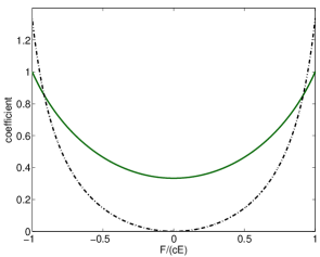
(a) Convection coefficients.

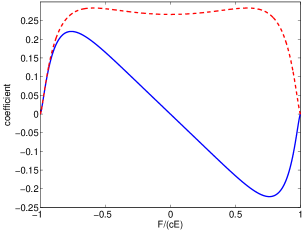
(b) Diffusion coefficients.

Figure 1: Perturbed M1 model coefficients. Left: $\chi$ (dark green solid line) and $\eta$ (black dash-dot line). Right: $D_{E}$ (blue solid line) and $D_{F}$ (red dashed line).

5 Numerical Simulation using Discontinuous Galerkin

In slab geometries, the diffusion-corrected $M_{1}$ model and the material energy (6) reduce to

$$\partial_{t}\mathbf{u}+\partial_{x}\mathbf{f}(\mathbf{u},\partial_{x}\mathbf{u}) =\mathbf{s}(\mathbf{u}),\quad(x,t)\in(x_{L},x_{R})\times(0,t_{\text{final}}),$$ (47a)

$$\partial_{t}T =\frac{c\sigma_{\mathrm{a}}}{C_{v}}(E-aT^{4}),$$ (47b)

where

$$\mathbf{u}=\begin{bmatrix}cE\\ F\end{bmatrix},\quad\mathbf{s}(\mathbf{u}) =\begin{bmatrix}-c^{2}\sigma_{\mathrm{a}}(E-aT^{4})+cS\\ -c\sigma_{\mathrm{t}}F\end{bmatrix},\quad\mathbf{f}(\mathbf{u},\partial_{x}\mathbf{u})=\begin{bmatrix}cF\\ c^{2}\Pi_{\delta}\end{bmatrix},$$ (47c)

$\Pi_{\delta}=\Pi^{\rm{M_{1}}}+\delta(\Pi^{\rm{C}}+\Pi^{\rm{D}})$ and $C_{v}=\frac{\partial e}{\partial T}$ is the specific heat at constant volume. In this setting, the convective flux of the $PM_{1}$ model is hyperbolic.

Proposition 2.

The perturbed $M_{1}$ system in slab geometry is hyperbolic if $\Pi^{\rm{D}}=0$ and $|F|<cE$.

Proof.

The proof is a direct calculation, given in the appendix. ∎

We simulate the system (47) using a Runge-Kutta discontinuous Galerkin (RKDG) method. The RKDG method is a method of lines: the DG discretization is only applied to spatial variables while time discretization is achieved by explicit Runge-Kutta time integrators. The presentation here is rather brief and relies on details found in [48], where the method was applied to the $M_{1}$ model. A general description of the RKDG method can be found, for example, in [17, 16].

5.1 Spatial Discretization

We divide the computational domain $(x_{L},x_{R})$ into $J$ cells with edges

$$x_{L}=x_{1/2}<x_{3/2}<\ldots<x_{J+1/2}=x_{R},$$

and let $x_{j}$ denote the center of each cell $I_{j}=(x_{j-1/2},x_{j+1/2})$. We let $h_{j}:=x_{j+1/2}-x_{j-1/2}$ be the length of the interval $I_{j}$ and set $h:=\max_{j}h_{j}$. We denote the finite-dimensional approximation space by

$$V_{h}^{k}=\{v\in L^{1}(x_{L},x_{R}):\,v_{|_{I_{j}}}\in{\cal P}^{k}(I_{j}),\,j=1,\dots,J\},$$

where ${\cal P}^{k}(I_{j})$ is the space of polynomials of degree at most $k$ on the interval $I_{j}$.

The semidiscrete DG scheme is derived from a weak formulation of (47). However, following [18] we first reduce the convection-diffusion equations (47) to a system of first-order equations by introducing the auxiliary variable $\mathbf{v}$:

$$\partial_{t}\mathbf{u}+\partial_{x}\mathbf{f}(\mathbf{u},\mathbf{v}) =\mathbf{s}(\mathbf{u}),$$ (48a)

$$\partial_{x}\mathbf{u} =\mathbf{v},$$ (48b)

$$\partial_{t}T =\frac{c\sigma_{\mathrm{a}}}{C_{v}}(E-aT^{4}).$$ (48c)

The exact solutions $\mathbf{u}(\cdot,t)$, $\mathbf{v}(\cdot,t)$ and $T(\cdot,t)$ are then replaced by approximations $\mathbf{u}_{h}(\cdot,t)$, $\mathbf{v}_{h}(\cdot,t)$ $\in V_{h}^{k}\times V_{h}^{k}$ and $T_{h}(\cdot,t)\in V_{h}^{k}$, and the resulting set of equations is required to hold for all test functions $b_{h}\in V_{h}^{k}$:

$$\int_{I_{j}}b_{h}(x)\partial_{t}\mathbf{u}_{h}(x,t)dx-\int_{I_{j}}\mathbf{f}(\mathbf{u}_{h}(x,t),\mathbf{v}_{h}(x,t))\partial_{x}b_{h}(x)dx$$ (49a)

$$+\left\llbracket\mathbf{f}b_{h}(x)\right\rrbracket_{j} =\int_{I_{j}}\mathbf{s}(\mathbf{u}_{h}(x,t))b_{h}(x)dx$$

$$\int_{I_{j}}b_{h}(x)\mathbf{v}_{h}(x,t)dx+\int_{I_{j}}\mathbf{u}_{h}(x,t)\partial_{x}b_{h}(x)dx-\left\llbracket\mathbf{u}b_{h}(x)\right\rrbracket_{j} =0$$ (49b)

$$\int_{I_{j}}b_{h}(x)\partial_{t}T_{h}(x,t)dx=\int_{I_{j}}b_{h}(x)\frac{c\sigma_{\mathrm{a}}(x)}{C_{v}}(E_{h}(x,t) -aT_{h}^{4}(x,t))dx.$$ (49c)

Here we use the bracket notation:

$$\left\llbracket\mathbf{f}b_{h}(x)\right\rrbracket_{j}=\mathbf{f}_{j+1/2}b_{h}(x_{j+1/2}^{-})-\mathbf{f}_{j-1/2}b_{h}(x_{j-1/2}^{+})$$ (50)

where

$$\mathbf{f}_{j\pm 1/2}(\mathbf{u},\mathbf{v})=\mathbf{f}(\mathbf{u}(x_{j\pm 1/2},t),\mathbf{v}(x_{j\pm 1/2},t))$$ (51)

and

$$b_{h}(x_{j+1/2}^{-})=\lim_{\varepsilon\to 0^{+}}b_{h}(x_{j+1/2}-\varepsilon),\quad b_{h}(x_{j-1/2}^{+})=\lim_{\varepsilon\to 0^{+}}b_{h}(x_{j-1/2}+\varepsilon)$$ (52)

are the right and left limits of $b_{h}$ at the cell interfaces $x_{j\pm 1/2}$. The term $\left\llbracket\mathbf{u}b_{h}(x)\right\rrbracket_{j}$ is defined in an analogous fashion.

Since the components of $\mathbf{u}_{h}(.,t)$ and $\mathbf{v}_{h}(.,t)$ are piecewise polynomials, the edge values of $\mathbf{u}$ and $\mathbf{v}$ in (51) are not strictly defined. Thus, the nonlinear flux function $\mathbf{f}$ is replaced by a numerical flux $\hat{\mathbf{f}}$ which depends on the pointwise limits of $\mathbf{u}_{h}$, $\mathbf{v}_{h}$ on either side of the edge at $x_{j\pm 1/2}$:

$$\hat{\mathbf{f}}_{j\pm 1/2}=\hat{\mathbf{f}}(\mathbf{u}_{h}(x^{-}_{j\pm 1/2},t),\mathbf{u}_{h}(x^{+}_{j\pm 1/2},t),\mathbf{v}_{h}(x^{-}_{j\pm 1/2},t),\mathbf{v}_{h}(x^{+}_{j\pm 1/2},t)).$$ (53)

The notations for $\hat{\mathbf{u}}$ carry over analogously.

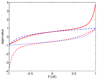
Figure 2: Eigenvalues of the hyperbolic flux Jacobian: M1 model (blue lines), perturbed M1 model (red lines).

It remains to choose suitable numerical fluxes $\hat{\mathbf{f}}$ and $\hat{\mathbf{u}}$. Since (47) has both a convective flux

$$\mathbf{f}^{\rm{C}}(\mathbf{u}):=\begin{bmatrix}cF\\ c^{2}\,\Pi^{\rm{M_{1}}}+\displaystyle\frac{c}{\sigma_{\mathrm{t}}}\eta(E,F)\left(c\sigma_{\mathrm{s}}E+c\sigma_{\mathrm{a}}aT^{4}+S\right)\end{bmatrix}$$ (54)

and a diffusive flux

$$\mathbf{f}^{\rm{D}}(\mathbf{u},\mathbf{v})=\begin{bmatrix}0\\ c^{2}\,{\bf D}(\mathbf{u})\cdot\mathbf{v}\end{bmatrix}\>$$ (55)

the choice is not obvious. Several approaches have been presented in literature [6, 57, 40, 46]. In [6], the prescription for the diffusive term is given by

$$\hat{\mathbf{f}}^{\rm{D}}_{j\pm 1/2} =\frac{1}{2}\left[\mathbf{f}^{\rm{D}}(\mathbf{u}^{-}_{j\pm 1/2},\mathbf{v}^{-}_{j\pm 1/2})+\mathbf{f}^{\rm{D}}(\mathbf{u}^{+}_{j\pm 1/2},\mathbf{v}^{+}_{j\pm 1/2})\right],$$ (56)

$$\hat{\mathbf{u}}_{j\pm 1/2} =\frac{1}{2}\left[\mathbf{u}_{j\pm 1/2}^{-}+\mathbf{u}_{j\pm 1/2}^{+}\right].$$ (57)

Combining this term with the Lax-Friedrichs flux for $\mathbf{f}^{\rm{C}}(\mathbf{u})$ gives the following total numerical flux:

$$\hat{\mathbf{f}}_{j\pm 1/2}=\frac{1}{2}\left[\mathbf{f}(\mathbf{u}_{j\pm 1/2}^{-},\mathbf{v}_{j\pm 1/2}^{-})+\mathbf{f}(\mathbf{u}_{j\pm 1/2}^{+},\mathbf{v}_{j\pm 1/2}^{+})-\lambda(\mathbf{u}_{j\pm 1/2}^{+}-\mathbf{u}_{j\pm 1/2}^{-})\right]\,,$$ (58)

where $\lambda$ is the largest magnitude of any eigenvalue of the Jacobian associated with $\mathbf{f}^{\rm{C}}$. These eigenvalues, in general, depend on material properties, the temperature $T$ and the source term $S$. In contrast to the M1 model, they are not bounded by the speed of light $c$. For example, neglecting the temperature and source the maximum value is approximately $9.12\,c$. We instead use the smaller value of $\lambda=c$, which is the particle speed in the transport equation and is consistent with the application of the control parameter to enforce realizability (see Section 3.3). Figure 2 shows the comparison of eigenvalues for the M1 and perturbed M1 modeling when $c=1$, $\sigma_{\mathrm{s}}=1$, $\sigma_{\mathrm{t}}=3$, $T=0=S$.

The DG solutions $\mathbf{u}_{h}$, $\mathbf{v}_{h}$ and $T_{h}$ are expanded in terms of local basis functions $\{b^{j}_{l}\}_{l=0}^{k}$ for ${\cal P}^{k}(I_{j})$ in each cell $I_{j}$:

$$\mathbf{u}^{j}_{h}(x,t)=\sum_{l=0}^{k}\mathbf{u}^{j}_{l}(t)b^{j}_{l}(x),\quad\mathbf{v}^{j}_{h}(x,t)=\sum_{l=0}^{k}\mathbf{v}^{j}_{l}(t)b^{j}_{l}(x),\quad T^{j}_{h}(x,t)=\sum_{l=0}^{k}T^{j}_{l}(t)b^{j}_{l}(x)\quad\text{for }x\in I_{j}.$$

The standard choice of basis for ${\cal P}(I_{j})$ is generated by Legendre polynomials $P_{l}$ that are defined on the reference cell $[-1,1]$:

$$b^{j}_{l}(x)=P_{l}\left(\frac{2(x-x_{j})}{h_{j}}\right)\>,\quad j\in\{1,\dots,J\}\,,l\in\{0,\dots,k\}\>,$$ (59)

and normalized so that

$$\int_{-1}^{1}P_{l}(y)P_{m}(y)dy=\frac{2}{2m+1}\delta_{l,m}.$$ (60)

With $\xi_{j}(y):=x_{j}+yh_{j}/2$, this gives a formulation defined on the reference cell:

$$\frac{h_{j}}{2m+1}\partial_{t}\mathbf{u}^{j}_{m}(t)-\int_{-1}^{1}\mathbf{f}(\mathbf{u}^{j}_{h}(\xi_{j}(y),t),\mathbf{v}^{j}_{h}(\xi_{j}(y),t))\partial_{y}P_{m}(y)dy$$ (61a)

$$\hskip 85.35826pt+\hat{\mathbf{f}}_{j+1/2}-(-1)^{m}\hat{\mathbf{f}}_{j-1/2}=\frac{h_{j}}{2}\int_{-1}^{1}\mathbf{s}(\mathbf{u}^{j}_{h}(\xi_{j}(y),t))P_{m}(y)dy,$$

$$\frac{h_{j}}{2m+1}\mathbf{v}^{j}_{m}(t)+\sum_{l=0}^{k}\mathbf{u}_{l}^{j}(t)\>{\cal C}_{l,m}-\hat{\mathbf{u}}_{j+1/2}+(-1)^{m}\hat{\mathbf{u}}_{j-1/2}=0,$$ (61b)

$$\frac{h_{j}}{2m+1}\partial_{t}T_{m}^{j}(t)=\frac{ch_{j}}{2C_{v}}\sum_{l=0}^{k}E_{l}^{j}(t)\left(\int_{-1}^{1}P_{m}(y)P_{l}(y)\sigma_{\mathrm{a}}(\xi_{j}(y))\right)dy$$ (61c)

$$\hskip 256.0748pt-\frac{ach_{j}}{2C_{v}}\int_{-1}^{1}P_{m}(y){T_{h}^{j}}^{4}(\xi_{j}(y),t)\sigma_{\mathrm{a}}(y)dy,$$

where

$${\cal C}_{l,m}=\int_{-1}^{1}P_{l}(y)\partial_{y}P_{m}(y)dy.$$ (62)

The remaining integrals are calculated by a quadrature rule. Note that (61b) can be solved locally for $\mathbf{v}^{j}_{m}(t)$ in each cell $I_{j}$, which can then be substituted back into (61a).

5.2 Time Discretization: Explicit SSP Runge-Kutta Schemes

The purpose of high-order, strong stability preserving (SSP) Runge-Kutta time integration methods is to achieve high-order accuracy in time while preserving desirable properties of the forward Euler method (for a review, see [25]). In this paper, we only use explicit schemes, which compute values of the unknowns at several intermediate stages. Each stage is a convex combination of forward Euler operators and this usually leads to modified CFL restrictions.

The equations in (61) form a system of ODEs for the coefficients $\mathbf{u}^{j}_{m}(t)$ and $T_{m}^{j}(t)$. For all $j\in\{1,\ldots,J\}$ and $m\in\{0,\ldots,k\}$, we write this system in the abstract form:

$$\partial_{t}\mathbf{u}^{j}_{m}(t) ={\cal L}^{j}_{\mathbf{u},m}(\mathbf{u}^{j-1}_{0},\ldots,\mathbf{u}^{j-1}_{k},\mathbf{u}^{j}_{0},\ldots,\mathbf{u}^{j}_{k},\mathbf{u}^{j+1}_{0},\ldots,\mathbf{u}^{j+1}_{k}),$$ (63)

$$\partial_{t}T^{j}_{m}(t) ={\cal L}^{j}_{T,m}(E^{j}_{0},\ldots,E^{j}_{k},T^{j}_{0},\ldots,T^{j}_{k}).$$ (64)

Here, ${\cal L}^{j}_{\mathbf{u},m}$ and ${\cal L}^{j}_{T,m}$ are the respective right-hand sides of the ODEs.

Let $\{t^{n}\}_{n=0}^{N}$ be an equidistant partition of $[0,t_{\text{final}}]$ and set $\Delta t:=t_{\text{final}}/N$. Let $\Lambda$ denote the application of a generic slope limiter, and let $\pi_{V^{m}_{h}}$ be the orthogonal projection onto the finite dimensional space $V_{h}^{m}$. Note that $\Lambda$ is applied at every Runge-Kutta stage. The algorithm for the optimal third-order SSP Runge-Kutta (SSPRK(3,3)) method [56] reads as follows:

• For all $j\in\{1,\ldots,J\}$ and $m\in\{0,\ldots,k\}$, set $\mathbf{u}_{m}^{j,0}=\Lambda\{\pi_{V^{m}_{h}}(\mathbf{u}_{0})\}$.

• For all $n\in\{0,\ldots,N-1\}$, $j\in\{1,\ldots,J\}$, and $m\in\{0,\ldots,k\}$,

  1. Compute the intermediate stages

     $$\mathbf{u}_{m}^{j,(1)} =\Lambda\left\{\mathbf{u}_{m}^{j,n}+\Delta t{\cal L}^{j}_{\mathbf{u},m}(\mathbf{u}_{h}^{j,(0)})\right\}$$

     $$\mathbf{u}_{m}^{j,(2)} =\Lambda\left\{\frac{3}{4}\mathbf{u}_{m}^{j,n}+\frac{1}{4}\mathbf{u}_{m}^{j,(1)}+\frac{1}{4}\Delta t{\cal L}^{j}_{\mathbf{u},m}(\mathbf{u}_{h}^{j,(1)})\right\}$$ (65)

     $$\mathbf{u}_{m}^{j,(3)} =\Lambda\left\{\frac{1}{3}\mathbf{u}_{m}^{j,n}+\frac{2}{3}\mathbf{u}_{m}^{j,(2)}+\frac{2}{3}\Delta t{\cal L}^{j}_{\mathbf{u},m}(\mathbf{u}_{h}^{j,(2)})\right\}$$

  2. Set $\mathbf{u}_{m}^{j,n+1}=\mathbf{u}_{m}^{j,(3)}$.

For the sake of completeness, we also state the optimal fourth order scheme SSPRK(5,4) [25]:

$$\mathbf{u}_{m}^{j,(1)} =\Lambda\{\mathbf{u}_{h}^{(n)}+0.391752226571890\,\Delta t\,{\cal L}^{j}_{\mathbf{u},m}(\mathbf{u}_{m}^{j,(n)})\}$$

$$\mathbf{u}_{m}^{j,(2)} =\Lambda\{0.444370493651235\,\mathbf{u}_{m}^{j,(n)}+0.555629506348765\,\mathbf{u}_{m}^{j,(1)}$$

$$\quad+0.368410593050371\,\Delta t\,{\cal L}^{j}_{\mathbf{u},m}(\mathbf{u}_{m}^{j,(1)})\}$$

$$\mathbf{u}_{m}^{j,(3)} =\Lambda\{0.620101851488403\,\mathbf{u}_{m}^{j,(n)}+0.379898148511597\,\mathbf{u}_{m}^{j,(2)}$$

$$\quad+0.251891774271694\,\Delta t\,{\cal L}^{j}_{\mathbf{u},m}(\mathbf{u}_{m}^{j,(2)})\}$$ (66)

$$\mathbf{u}_{m}^{j,(4)} =\Lambda\{0.178079954393132\,\mathbf{u}_{m}^{j,(n)}+0.821920045606868\,\mathbf{u}_{m}^{j,(3)}$$

$$\quad+0.544974750228521\,\Delta t\,{\cal L}^{j}_{\mathbf{u},m}(\mathbf{u}_{m}^{j,(3)})\}$$

$$\mathbf{u}_{h}^{(n+1)} =\Lambda\{0.517231671970585\,\mathbf{u}_{m}^{j,(2)}+0.096059710526147\,\mathbf{u}_{m}^{j,(3)}$$

$$\quad+0.386708617503269\,\mathbf{u}_{m}^{j,(4)}+0.063692468666290\,\Delta t\,{\cal L}^{j}_{\mathbf{u},m}(\mathbf{u}_{m}^{j,(3)})$$

$$\quad+0.226007483236906\,\Delta t\,{\cal L}^{j}_{\mathbf{u},m}(\mathbf{u}_{m}^{j,(4)})\}.$$

Note that SSPRK(3,3) permits a timestep of the same size as forward Euler, while the SSPRK(5,4) method is less restrictive, allowing for a time step that is $1.508$ times larger the forward Euler scheme.

5.3 Limiters

As in [48], two types of limiters are used. The first is standard; it is used to suppress spurious oscillations and maintain stability. There are many such limiters available. In this paper, we apply the moment limiter from [12], which is a modification of the original limiter in [7]. This limiter is applied to the variables $\mathbf{u}$, but not the auxiliary variables $\mathbf{v}$ or the temperature $T$. Additional details can be found in [48].

5.3.1 Realizability-Preserving Limiter

The second limiter is a realizability-preserving limiter which is needed to ensure that the cell averages of $E$ and $F$ satisfy the realizability condition (1) at each stage of the numerical computation. The limiter is based on the work from [67] and [66] and is very similar to what was done in [48] for the $M_{1}$ model. The major difference here is the addition of the control parameter $\delta$.

An essential ingredient of the realizability limiter is the Gauss-Lobatto quadrature set

$$\{x_{j-1/2}=\hat{x}_{j}^{1},\hat{x}_{j}^{2},\ldots,\hat{x}_{j}^{M-1},\hat{x}_{j}^{M}=x_{j+1/2}\}\subset I_{j},$$ (67)

where, for a spatial reconstruction of order $k$, $M$ is the smallest integer such that $2M-3\geq 2k+1$. This condition on $M$ ensures accuracy of the scheme [15]. The weaker condition $2M-3\geq k$ ensures that the quadrature integrates elements of the approximation space $V_{h}^{k}$ exactly.

The realizability limiter is defined in order to ensure that $\mathbf{u}_{h}(\hat{x}_{j}^{\ell})\in\mathcal{R}_{2}$ at each point $\hat{x}_{j}^{\ell}$ in the quadrature set. However, we enforce the convexity condition indirectly by requiring the positivity of the intermediate quantities

$$Q:=\frac{cE+F}{2}\quad\mbox{and}\quad R:=\frac{cE-F}{2}\>.$$ (68)

The inverse transformation that maps $(Q,R)\mapsto(cE,F)$ is given by

$$E=\frac{Q+R}{c}\quad\mbox{and}\quad F=Q-R\>.$$ (69)

An additional limiter is also used to enforce the positivity of the temperature reconstruction at each quadrature point.

We now proceed to define the limiters. Let $\mathbf{u}_{h}^{j,n}=(cE_{h}^{j,n},F_{h}^{j,n})$ and $T_{h}^{j,n}$ be the approximations of $\mathbf{u}$ and $T$ in cell $I_{j}$ at time $t^{n}$, and let $\hat{\mathbf{u}}_{h}^{j,n}$ and $\hat{T}_{h}^{j,n}$ denote the modifications of $\mathbf{u}_{h}^{j,n}$ and $T_{h}^{j,n}$ that are generated by the limiting. We assume that the cell average of $\mathbf{u}_{h}^{j,n}$, which we denote by $\overline{\mathbf{u}}_{h}^{j,n}$, is realizable, i.e., $\overline{\mathbf{u}}_{h}^{j,n}\in{\cal R}_{2}$. We also assume that the cell average of $T_{h}^{j,n}$, which we denote by $\overline{T}_{h}^{j,n}$, is positive. Let $Q_{h}^{j,n}(x)$ and $R_{h}^{j,n}(x)$ be the approximations of $Q$ and $R$, respectively, and define limited variables by

$$\hat{Q}_{h}^{j,n}(x) =\theta^{j,n}_{Q}Q_{h}^{j,n}(x)+(1-\theta^{j,n}_{Q})\overline{Q}_{h}^{j,n}\>,$$ (70a)

$$\hat{R}_{h}^{j,n}(x) =\theta^{j,n}_{R}R_{h}^{j,n}(x)+(1-\theta^{j,n}_{R})\overline{R}_{h}^{j,n}\>,$$ (70b)

$$\hat{T}_{h}^{j,n}(x) =\theta^{j,n}_{T}T_{h}^{j,n}(x)+(1-\theta^{j,n}_{T})\overline{T}_{h}^{j,n}\>,$$ (70c)

where

$$\theta^{j,n}_{Q} :=\min\left\{\frac{\overline{Q}_{h}^{j,n}-\varepsilon/2}{\overline{Q}_{h}^{j,n}-Q^{j,n}_{\min}},1\right\}\,,\quad Q^{j,n}_{\min}:=\min_{\ell=1,\ldots,M}Q^{j,n}_{h}({\hat{x}}_{j}^{\ell})\>,$$ (70d)

$$\theta^{j,n}_{R} :=\min\left\{\frac{\overline{R}_{h}^{j,n}-\varepsilon/2}{\overline{R}_{h}^{j,n}-R^{j,n}_{\min}},1\right\}\,,\quad R^{j,n}_{\min}:=\min_{\ell=1,\ldots,M}R^{j,n}_{h}({\hat{x}}_{j}^{\ell})\>,$$ (70e)

$$\theta^{j,n}_{T} :=\min\left\{\frac{\overline{T}_{h}^{j,n}}{\overline{T}_{h}^{j,n}-T^{j,n}_{\min}},1\right\}\,,\quad T^{j,n}_{\min}:=\min_{\ell=1,\ldots,M}T^{j,n}_{h}({\hat{x}}_{j}^{\ell})\>.$$ (70f)

The parameter $\varepsilon>0$ is chosen to maintain numerical stability with finite precision arithmetic; its value should be small relative to the magnitude of the variables in a given problem. The components of $\hat{\mathbf{u}}_{h}^{j,n}$ are then defined using (69). They satisfy the following property which is a key ingredient for maintaining realizability in the RKDG scheme.

Lemma 3 ([48]).

If $\overline{\mathbf{u}}_{h}^{j,n}\in\mathcal{R}_{2}$ (respectively: $\overline{T}_{h}^{j,n}\geq 0$), then $\hat{\mathbf{u}}_{h}^{j,n}(\hat{x}_{j}^{\ell})\in\mathcal{R}_{2}^{\varepsilon}:=\mathcal{R}_{2}+[\varepsilon,0]^{T}$ (respectively: $\hat{T}_{h}^{j,n}(\hat{x}_{j}^{\ell})\geq 0$) for $\ell=1,\ldots,M$.

5.3.2 Setting the Control Parameter

We now define the control parameter $\delta$, discussed in Section 3.3. Our definition is guided by the following result.

Lemma 4 ([48]).

In the one dimensional setting, a necessary condition for $(cE,F,c\Pi_{\delta})\in\mathcal{R}_{3}$ is that

• $\Pi_{\delta}\leq E$,

• $|F\pm c\Pi_{\delta}|\leq cE\pm F$.

Rather than to require $(cE,F,c\Pi_{\delta})\in\mathcal{R}_{3}$, we choose $\delta\in[0,1]$ to ensure the weaker conditions (C1) and (C2). More specifically, for any $(cE,F)\in\mathcal{R}_{2}$, we set

$$\delta(E,F) =\begin{cases}\delta_{0}(E,F),\quad&\Pi^{\rm{C}}(E,F)+\Pi^{\rm{D}}(E,F)>0,\\ \delta_{1}(E,F),\quad&\Pi^{\rm{C}}(E,F)+\Pi^{\rm{D}}(E,F)<0,\\ \end{cases}$$ (71a)

where

$$\delta_{0}=\min\left\{\frac{E-\Pi^{\rm{M_{1}}}}{\Pi^{\rm{C}}+\Pi^{\rm{D}}},1\right\},\quad\delta_{1} =\min\left\{\frac{-2F+cE+c\Pi^{\rm{M_{1}}}}{c|\Pi^{\rm{C}}+\Pi^{\rm{D}}|},\frac{2F+cE+c\Pi^{\rm{M_{1}}}}{c|\Pi^{\rm{C}}+\Pi^{\rm{D}}|},1\right\}.$$ (71b)

Lemma 5.

For all $(cE,F)\in\mathcal{R}_{2}$, $\Pi_{\delta}:=\Pi^{\rm{M_{1}}}+\delta[\Pi^{\rm{C}}+\Pi^{\rm{D}}]$ satisfies (C1) – (C2).

Proof.

The assertion $(cE,F)\in\mathcal{R}_{2}$ implies $(cE,F,c\Pi^{\rm{M_{1}}})\in\mathcal{R}_{3}$. It follows then that for $\Pi^{\text{D}}=0$, conditions (C1) – (C2) are trivially satisfied. It remains only to show the following inequalities:

$$c\Pi_{\delta}\leq cE\quad\mbox{and}\quad c\Pi_{\delta}\geq 2F-cE\quad\mbox{and}\quad c\Pi_{\delta}\geq-2F-cE.$$ (72)

These relations are easily verified by applying the definition of $\delta$ and using the fact that $(cE,F,c\Pi^{\rm{M_{1}}})\in\mathcal{R}_{3}$. ∎

With $\delta$ given by (71), one can show that cell averages of $\mathbf{u}_{h}$ remain realizable and that the cell average of $T_{h}$ remains positive in a forward Euler step. Let

$$\mathbf{u}^{j,n}_{\ell}:=\mathbf{u}_{h}^{j,n}({\hat{x}}_{j}^{\ell})\>,\quad T^{j,n}_{\ell}:=T_{h}^{j,n}({\hat{x}}_{j}^{\ell})\>,\quad\Pi_{\delta,\ell}^{j,n}:=\Pi_{\delta}(\mathbf{u}^{j,n}_{\ell})\>,\quad\sigma_{\mathrm{t,\ell}}:=\sigma_{\mathrm{t}}({\hat{x}}_{j}^{\ell}).$$ (73)

Lemma 6.

Assume that $2M-3\geq k$ and for each $\ell=1,\ldots,M$, that

$$\mathbf{u}^{j,n}_{\ell}\in{\cal R}_{2},\quad T^{j,n}_{\ell}\geq 0$$ (74)

and $\Pi_{\delta,\ell}^{j,n}$ satisfies (C1) and (C2). Assume further that $\Delta t$ satisfies the following conditions:

• $\displaystyle\Delta t<\min_{\ell=1,\ldots,M}{\left\{\frac{1}{c\sigma_{\mathrm{t,\ell}}}\right\}}$,

• $\displaystyle\Delta t<\min_{\ell=1,\ldots,M}{\left\{\frac{w_{\ell}h}{c(1+w_{\ell}\sigma_{\mathrm{t,\ell}}h)}\right\},}$

• $\displaystyle\Delta t\leq\min_{\ell=1,\ldots,M}{\left\{\frac{C_{v}}{\sigma_{\mathrm{a,\ell}}ac(T^{j,n}_{\ell})^{3}}\right\}.}$

where $h:=\min_{j}h_{j}$. Then after a forward Euler time step,

$$\overline{\mathbf{u}}_{h}^{j,n+1}\in{\cal R}_{2}\quad\mbox{and}\quad\overline{T}^{j,n+1}_{h}\geq 0.$$ (75)

Proof.

We refer the reader to the proof of Theorem 3 in [48] for the $M_{1}$ model, which relies exactly on the conditions (A1)–(A3) and (C1)–(C2). The only difference is that (C1) and (C2) are assumed in Lemma 6, while in [48] they are naturally satisfied by the $M_{1}$ model. ∎

Theorem 2.

The Runge-Kutta discontinuous Galerkin scheme which combines

1. the space discretization in (61),

2. the limiters in (70),

3. the modified pressure $\Pi_{\delta}$ in (47) with control parameter $\delta$ given by (71),

4. a strong-stability-preserving Runge Kutta time integrator, and

5. a sufficiently accurate Gauss-Lobatto quadrature

preserves the realizability of the moments in the sense of cell averages. In particular, if the time step conditions (A1)-(A2) in the statement of Lemma 6 hold and if $\overline{\mathbf{u}}^{j,n}_{h}\in\mathcal{R}_{2}$, then $\overline{\mathbf{u}}^{j,n+1}_{h}\in\mathcal{R}_{2}$.

Proof.

Application of the limiters in (70) ensures that the conditions of Lemma 6 hold at each stage in the SSP-RK scheme. Each successive stage is an application of the forward Euler operator to the current stage with an appropriately modified time step. Thus, the conclusions of Lemma 6 apply at the next stage, including the final stage, which gives $\mathbf{u}^{j,n+1}_{h}$. ∎

6 Numerical Results

In this section, we present several numerical computations in slab geometry for a choice of test cases that are common for the $M_{1}$ model. The goal is to compare and contrast the perturbed $M_{1}$ model with the $M_{1}$ model and to point out benefits and drawbacks. Benchmark solutions are generated by the discrete ordinates method with an upwind scheme in space, high-order spherical harmonics or semi-analytic expressions. The RKDG implementation has been verified and benchmarked in [48]. The correct implementation of the additional perturbative terms has been checked by the method of manufactured solutions [53].

As in [48] our algorithm is implemented in MATLAB, and Gauss-Lobatto quadrature on [-1,1] is used. Additionally, the Runge-Kutta time integration methods as well as parameters for the admissibility limiter are applied in the same way. In order to satisfy the conditions of Lemma 6 and to guarantee stability, the time step is set to

$$\Delta t<\min\left\{c_{1},c_{2},c_{3},c_{4}\right\},$$ (76a)

$$c_{1}=\frac{1}{c\sigma_{\mathrm{t,\text{max}}}}\>,\quad c_{2}= \frac{h\,w_{\text{min}}}{c(1+w_{\text{max}}\sigma_{\mathrm{t,\text{max}}}\,h)}\>,\quad c_{3}=\frac{C_{v}}{ac\tau_{\text{max}}}\>\quad\mbox{and}\quad c_{4}=\frac{h^{2}}{2(2k+1)},$$ (76b)

where $k$ is the polynomial degree, $h=\min_{j}h_{j}$, $w_{\text{min}}$ and $w_{\text{max}}$ are the minimum and maximum quadrature weights, respectively. The quantities $\sigma_{t,\text{max}}$ and $\tau_{\text{max}}$ are the maximum values of $\sigma_{\mathrm{t,\ell}}$ and $\sigma_{\mathrm{a,\ell}}(T_{\ell}^{j,n})^{3}$.

The constant $c_{4}$ is not needed to preserve realizability of the moments but rather to enforce a parabolic CFL condition. Without this condition, unstable modes grow without bound until the control parameter $\delta$ turns on and damps them. Unfortunately, the parabolic CFL restriction leads to small time steps.

The stability parameter for the realizability limiter of $E$ and $F$ is set to $\varepsilon=10^{-10}$. The same value is also used to enforce conditions (C1) and (C2), i.e., the control parameter in (71) is chosen such that

$$c\Pi_{\delta}\leq cE-\varepsilon\quad\mbox{and}\quad|F\pm c\Pi_{\delta}|\leq cE\pm F\pm\varepsilon.$$

In Sections 6.1-6.3, we study simulations with $c=1$ and neglect the energy equation which is included in the last two cases from Section 6.4. Unless otherwise stated, slope and realizability limiters are always turned on for all DG calculations. If transformation to characteristic variables for the slope limiter is used, it will be explicitly stated.

6.1 Two-Beam Instability

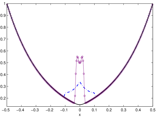
(a) $t=0.6$

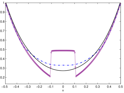
(b) $t=3$

Figure 3: Plots of E for the two-beam instability. $J=200$, $k=2$: $M_{1}$ (purple circle line), perturbed $M_{1}$ (blue dash-dot line), transport (black solid line).

We consider two incoming beams at the boundaries of the domain $[-0.5,0,5]$ and set $c=1$, $S=0$. Particles stream from both boundaries in a purely absorbing material with $\sigma_{a}=4=\sigma_{\mathrm{t}}$ and meet at $x=0$. We avoid getting too close to the boundary of the realizability domain and represent these beams in our moment model using the boundary conditions

$$\mathbf{u}(0,t)=[1,0.9999]^{T},\quad\mathbf{u}(1,t)=[1,-0.9999]^{T},\quad t>0$$

and initial conditions

$$\mathbf{u}_{0}(x)=[2\varepsilon,0]^{T},\quad x\in(-0.5,0,5).$$

For this problem, coupling to the material is ignored, and the material energy equation is not included in the simulation.

In Figure 3, one can observe the formation of a shock in the $M_{1}$ solution which persists at the steady-state. The perturbed $M_{1}$ model also develops an unphysical transient profile in which the particle number jumps in the center of the domain. While this artifact persists, the steady state solution ($t=3$) appears continuous. The steady-state solution also has noticeable kinks in the at $x\approx\pm 0.3$. For comparison, discrete ordinates solutions are plotted for which $256$ discretization points in angle and $1000$ points in space are used. The perturbed $M_{1}$ is throughout closer to the transport solution.

Remark 2.

Precise explanations for the occurrence of shocks and kinks in the perturbed $M_{1}$ solution require an additional analysis. For example, an explanation for the formation of shocks in the $M_{1}$ model is given [10]. However, such an analysis goes beyond the purpose of this paper and will be postponed to future work.

6.2 Source-Beam Problem

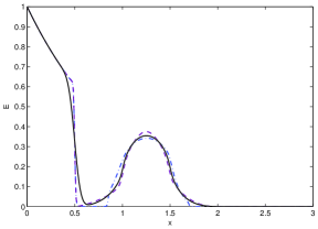
(a) $t=0.5$

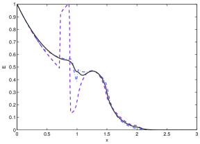
(b) $t=1$

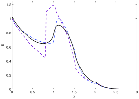
(c) $t=2$

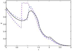
(d) $t=4$

Figure 4: Plots of E for the Source-beam problem. $J=300$, $k=2$: $M_{1}$ (purple dashed line), perturbed $M_{1}$ (blue dash-dot line), transport solution (black solid line)

In this problem, an incoming beam

$$\mathbf{u}(0,t)=[1,0.9999]^{T},\quad t>0,$$

on the left boundary of the domain $[0,3]$ hits an isotropic source $S=1/2$ generating particles on the interval $1\leq x<1.5$. In order to avoid complications of spatial discontinuities in the fluxes [65, 64, 41], we smooth the source and material cross sections, which enter into the perturbative components of the flux. The source $S$ is smoothed at the end points $x=1$ and $x=1.5$

$$S=\begin{cases}\frac{1}{4}(1+p_{H}(\frac{x-1}{\Delta})),&1-\Delta\leq x\leq 1+\Delta\\ \frac{1}{2},&1+\Delta<x<1.5-\Delta\\ \frac{1}{4}(1-p_{H}(\frac{x-1.5}{\Delta})),&1.5-\Delta\leq x\leq 1.5+\Delta\\ 0,&\text{else}\end{cases}$$ (77)

Similarly, we design the material properties with the cross sections:

$$\sigma_{\mathrm{a}} =\begin{cases}1,&0\leq x<2-\Delta\\ (1-p_{H}(\frac{x-2}{\Delta}))/2,&2-\Delta\leq x\leq 2+\Delta\\ 0,&\text{else}\end{cases},\quad\mbox{and}\quad$$ (78)

$$\sigma_{\mathrm{s}} =\begin{cases}1+p_{H}(\frac{x-1}{\Delta}),&1-\Delta\leq x\leq 1+\Delta\\ 2,&1+\Delta<x<2-\Delta\\ 2+4(1+p_{H}(\frac{x-2}{\Delta})),&2-\Delta\leq x\leq 2+\Delta\\ 10,&2+\Delta<x\leq 3\\ 0,&\text{else.}\end{cases}$$ (79)

The function $p_{H}$ is a Hermite polynomial of order 10 with $p_{H}(\pm 1)=\pm 1$ and $p^{(k)}_{H}(\pm 1)=0$ for $k=1,2,3,4$. If $p_{H}$ is extended by $\pm 1$ respectively, it is a $C^{4}$ function. The material property functions are illustrated in Figure 5.

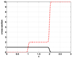
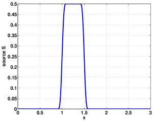
Figure 5: Source-beam problem. Material properties with $\Delta=0.05$: $\sigma_{s}$ (red dashed line), $\sigma_{a}$ (black solid line), $S$ (blue solid line)

On the right boundary, particles are absorbed and zero Dirichlet conditions

$$\mathbf{u}(3,t)=[\varepsilon,0]^{T},\quad t>0,$$ (80)

are set. Initially, there are (almost) no particles in the system, i.e.,

$$\mathbf{u}(x,0)=[\varepsilon,0]^{T},\quad x\in(0,3).$$ (81)

The value of $c$ is again set to one.

The perturbed $M_{1}$ results are compared to $M_{1}$ and transport solutions. Classic $M_{1}$ calculations are performed using the DG method from [48], with the same computational parameters as the $PM_{1}$ model and slope limiting performed in the characteristic variables. The transport solution is computed using the discrete ordinates method with $600$ spatial cells and $256$ discrete angles.

One can observe in Figure 4 that as time increases, particles entering from the left boundary encounter the source in the interior. As this happens the $M_{1}$ profile diverges from the transport solution. Even as steady state is achieved at $t=4$, there is a large difference for $x\leq 1$. The $PM_{1}$ profile agrees much better with the transport solution.

6.3 Gaussian Source

The next test case simulates particles with an initial energy density that is a Gaussian distribution in space and a zero energy density flux:

$$\mathbf{u}(x,0)=\left[\frac{1}{\xi\sqrt{2\pi}}\,e^{-\frac{x^{2}}{2\xi^{2}}},0\right]^{T},\quad\xi=0.1,\quad x\in(-L,L).$$

Periodic boundary conditions on $[-L,L]$ are prescribed where $L=t_{\text{final}}+1$. The computational domain is always chosen large enough to ensure that a negligible number of particles reaches the boundaries. No internal source is assumed (so $S=0$), and the medium is purely scattering with $\sigma_{\mathrm{s}}=\sigma_{\mathrm{t}}=1$. The velocity $c$ is also set to one and the material energy equation (6) is neglected. All DG results are computed with $h=0.01$ and polynomial degree $k=2$. For comparison, discrete ordinates solutions of the transport equations are obtained with $h=0.005$ and $128$ angular points.

Figure 6 displays the solutions at $t_{\text{final}}=1,2,3,10$. The $M_{1}$ model gives the expected wave effects that are washed out at larger times. These effects do not occur in the perturbed $M_{1}$ results. However, the $PM_{1}$ forms Gaussian bell that are higher and more narrow than the benchmark solution. At lower times, their maximum propagation speed is roughly half the correct velocity. Nevertheless, at $t_{\text{final}}=10$ the front of the $PM_{1}$ model catches up with the reference solution, at which point all three models agree reasonably well.

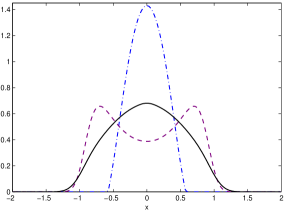
(a) $t_{\text{final}}=1$

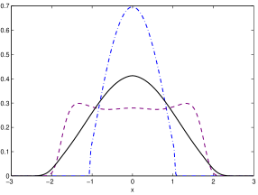
(b) $t_{\text{final}}=2$

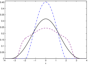
(c) $t_{\text{final}}=3$

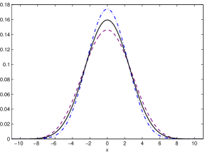
(d) $t_{\text{final}}=10$

Figure 6: Plots of E for the Gaussian source. $J=100\,(t_{\text{final}}+1)$, $k=2$: $M_{1}$ (purple circle line), perturbed $M_{1}$ (blue dash-dot line), transport (black solid line).

The perturbation $\tilde{\psi}$ from Section 3.2 is related to the difference between the $M_{1}$ and transport solution. Figure 6 indicates that this quantity is highly time-dependent. Additionally, the spatial gradient of $\tilde{\psi}$ is large at shorter times. Hence, this numerical example violates the smallness assumptions made in the derivation of the perturbed $M_{1}$ model in Section 3.2. Thus the lack of accuracy is not surprising.

6.4 Including the Material Energy Equation

The next two examples involve (2) coupling to the energy equation (6). The linearized Marshak wave problem from [61] is analyzed first and then a Marshak wave with material parameters taken from [48].

6.4.1 Smoothed Su-Olson’s Benchmark Problem

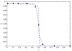
(a) $t=0.1$

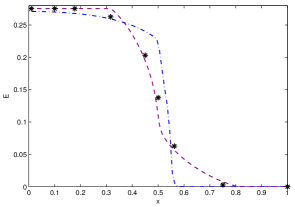
(b) $t=0.31623$

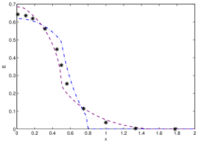
(c) $t=1$

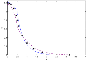
(d) $t=3.16228$

Figure 7: Plots of E for the Su-Olson Problem. $J=200$, $k=2$: $M_{1}$ (purple dashed line), perturbed $M_{1}$ (blue dash-dot line), semi-analytic (black asterisk).

In [61], tabulated data is provided for analytic solutions to a linearized Marshak wave problem, which serves as a validation of numerical algorithms in the radiative transfer community. In particular, this semi-analytic benchmark is also compared to diffusion-corrected $P_{N}$ approximations in [54]. It is therefore of interest to study solutions of the perturbed $M_{1}$ model to this problem.

We compute approximations to (2) and (6) in slab geometry with the following physical data

$$C_{v}=T^{3},\quad c=1,\quad\sigma_{\mathrm{a}}=1=\sigma_{\mathrm{t}}.$$

As in the source-beam problem, we seek to avoid the discontinuous material properties in [61] by introducing a smoothed version:

$$S(x,t)=\begin{cases}(1+p_{H}(\frac{x+0.5}{\Delta}))/2,&-0.5-\Delta\leq x\leq-0.5+\Delta,\\ 1,&-0.5+\Delta<x<0.5-\Delta,\\ (1-p_{H}(\frac{x-0.5}{\Delta}))/2,&0.5-\Delta\leq x\leq 0.5+\Delta,\\ 0,&\text{else,}\end{cases}$$

where $p_{H}$ is the Hermite polynomial described in Section 6.2. However, we still compare our numerical results to the semi-analytic solutions from [61] because the length of the smoothing window $2\Delta=0.02$ is relatively small.

Initially, the medium is cold and there is no radiation:

$$\psi(x,\mu,\nu,t=0)=0\quad\mbox{and}\quad T(x,t=0)=0.$$

Additionally, zero boundary conditions are enforced on an infinite domain:

$$\lim_{x\rightarrow\pm\infty}\psi(x,\mu,\nu,t)=0\quad\mbox{and}\quad\lim_{x\rightarrow\pm\infty}T(x,t)=0.$$

In practice, we impose periodic boundary conditions on a large domain $[-L,L]$ where $L=\lfloor t_{\rm{final}}\rfloor+1$.

Solutions at different times are provided in Figure 7 for the half plane $x\geq 0$. A grid size of $h=0.01$ and polynomial degree of $k=2$ are chosen for all DG solutions. Classic $M_{1}$ computations are slope limited in the characteristic variables. They are throughout close to the semi-analytic results. However at earlier times, the perturbed $M_{1}$ solutions have larger slopes at $x\approx 0.5$. There, the perturbed $M_{1}$ model yields larger deviations from the reference. Only at $t=3.16228$ solutions from both models are close to each other as well as to the semi-analytic points.

6.4.2 Thin Marshak Wave

In this problem, incoming radiation is prescribed on the left boundary by well-posed boundary conditions,

$$T(0,t) =1,\quad T(1,t)=0,\quad t>0,$$

$$\mathbf{u}(0,t) =[T(0,t)^{4}a,0.8\cdot T(0,t)^{4}ac]^{T},\quad\mathbf{u}(1,t)=[2\varepsilon,0]^{T},\quad t>0,$$

and the material is assumed to be purely absorbing:

$$\sigma_{\mathrm{a}}(T)=\frac{1}{(T+0.5)^{3}}\frac{\text{keV}^{3}}{\text{cm}},\quad\sigma_{s}=0,\quad S=0.$$

The physical constants are given by

$$c =3\cdot 10^{10}\,\text{cm/s} \text{speed of light},$$

$$a =1.372\cdot 10^{14}\,\text{erg/(cm}^{3}\text{keV}^{4}) \text{radiation constant},$$

$$C_{v} =3\cdot 10^{15}\,\text{erg/(cm}^{3}\text{keV)} \text{heat capacity},$$

which implies units of cm^-1 for cross sections and keV for temperature $T$. Initially, the material is cold

$$T_{0}(x) =5\cdot 10^{-4},\quad x\in(0,1),$$

$$\mathbf{u}(x,0) =[T_{0}(x)^{4}a,0]^{T},\quad x\in(0,1).$$

Due to above incoming radiation on the left boundary, radiation propagates through the medium from left to the right. The material temperature $T$ (Figure 8a) and the energy density $E$ (Figure 8a) decay smoothly to zero. The $M_{1}$ and $P\!M_{1}$ models yield very similar solutions. For comparison, a reference solution is computed using a $P_{99}$ model that is calculated with the DG method from [42]. The simulation of the $P_{99}$ model uses linear elements and $800$ spatial cells. The reference solution shows a much stronger decay in the energy and material temperature.

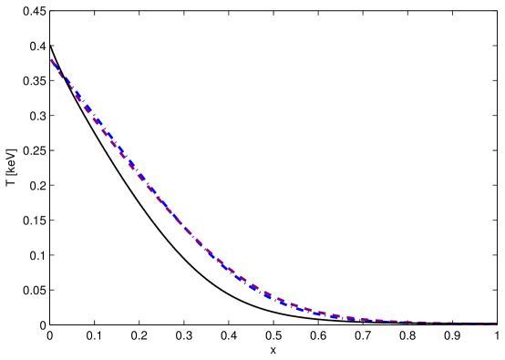
(a) Temperature at $t=0.1$ns.

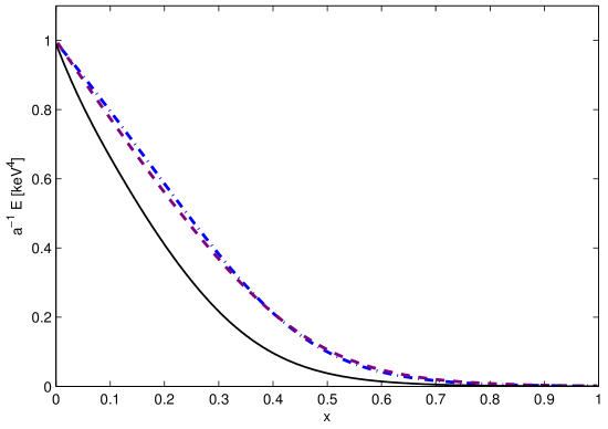
(b) Scaled scalar flux $a^{-1}E$ at $t=0.1$ns.

Figure 8: Thin Marshak wave. $J=160$, $k=2$: $M_{1}$ (purple dashed line), perturbed $M_{1}$ (blue dash-dot line), $P_{99}$ (black solid circle line).

7 Discussion and Conclusions

In this paper, we have derived a hierarchy of closures based on perturbations of well-known entropy-based closures. The derivation has been done in the context of grey photon transport. Our derivations reveals final equations containing an additional convective and diffusive term which are added to the flux term of the standard closure. This is different to perturbations to standard $P_{N}$ closures [54] which only gain a diffusive component.

For the first member of the hierarchy, the $P\!M_{1}$ model, we compute explicit formulas for all terms. The resulting system of equations is a convection-diffusion system which, for slab geometries, is discretized by using a Runge-Kutta discontinuous Galerkin method. By introducing a special limiter and an additional control parameter to modify the pressure term, we ensure that cell averages of the moments satisfy the important realizability property (1).

We perform simulations to compare qualitative results with the $M_{1}$ model and with highly-resolved discretizations of the original transport equation. Improvements to the standard $M_{1}$ model are observed in cases where unphysical shocks develop in the classical $M_{1}$ model. However, for problems with continuous solutions, there is little or no improvement; and in some cases, the $M_{1}$ model perform marginally better.

Finally, we discuss some open problems in this framework which might be addressed in future:

• Moment systems from entropy-based closures are known to be hyperbolic and satisfy a local dissipation law [35, 22], but such results are not yet known for the perturbed models. The partial result in Proposition 1 confirms that the additional diffusive term dissipates the entropy. Moreover, neglecting the diffusion contribution the system indeed becomes hyperbolic for the special case of the $M_{1}$ model in one dimension (i.e., for slab geometry).

• Standard issues in analysis such as existence and uniqueness of solutions have yet to be investigated for the $PM_{1}$ model or for PEB models in general.

• In Section 5.3.2, the control parameter $\delta$ is chosen to guarantee conditions (C1)-(C2). However, this ansatz is a crude modification of the original perturbative model and could distort numerical solutions. A more subtle approach, possibly along the lines of flux-limited diffusion, e.g. [39], would be preferable.

• An undesirable aspect of the RKDG method is the time step restriction required by the explicit time integrator. For convection-diffusion equations, stiff sources, and/or long time scales, this time step restriction is very harsh. To lower the computational effort, (semi-)implicit time discretizations are therefore necessary. In addition, the method does not address the challenges of spatially discontinuous fluxes that arise from discontinuities in sources and material cross-sections.

• Another issue is the formation of unphysical shocks in the (perturbed) $M_{1}$ solution. Further analysis is needed to understand why and when they appear and how to further mitigate them.

Appendix A Appendix

Computation of equation (29).

We first calculate two frequency integrals. Let $\kappa:=\frac{hc}{k}\hat{\boldsymbol{\alpha}}^{T}\mathbf{m}$ and $\theta:=-\kappa\nu$. Then

$${\int_{0}^{\infty}\eta_{*}^{\prime}\!\left(\frac{-h\nu c}{k}\hat{\boldsymbol{\alpha}}^{T}\mathbf{m}\right)\,d\nu}={\int_{0}^{\infty}\frac{2h\nu^{3}}{c^{2}}\frac{1}{\exp(-\kappa\nu)-1}\,d\nu}\\ =-\frac{2h}{c^{2}\kappa^{4}}{\int_{0}^{\infty}\frac{\theta^{3}}{\exp(\theta)-1}\,d\theta}=-\frac{2\pi^{4}h}{15c^{2}\kappa^{4}}$$ (82)

and

$${\int_{0}^{\infty}\eta_{*}^{\prime\prime}\!\left(\frac{-h\nu c}{k}\hat{\boldsymbol{\alpha}}^{T}\mathbf{m}\right)\,d\nu}={\int_{0}^{\infty}\frac{2h^{2}\nu^{4}}{kc}\frac{\exp(-\kappa\nu)}{[\exp(-\kappa\nu)-1]^{2}}\,d\nu}\\ =\frac{2h^{2}}{kc\kappa^{5}}{\int_{0}^{\infty}\frac{\theta^{4}\exp(\theta)}{[\exp(\theta)-1]^{2}}\,d\theta}=\frac{8\pi^{4}h^{2}}{15kc\kappa^{5}}.$$ (83)

With these two integrals, it is easy to show that $-\hat{\boldsymbol{\alpha}}/4$ is the unique solution to the linear system

$$\left\langle\mathbf{m}\mathbf{m}^{T}\eta_{*}^{\prime\prime}\!\left(\frac{-h\nu c}{k}\hat{\boldsymbol{\alpha}}^{T}\mathbf{m}\right)\right\rangle\boldsymbol{\beta}=\left\langle\mathbf{m}\eta_{*}^{\prime}\!\left(\frac{-h\nu c}{k}\hat{\boldsymbol{\alpha}}^{T}\mathbf{m}\right)\right\rangle,$$ (84)

so that

$$\left\langle\mathbf{m}\mathbf{m}^{T}\eta_{*}^{\prime\prime}\!\left(\frac{-h\nu c}{k}\hat{\boldsymbol{\alpha}}^{T}\mathbf{m}\right)\right\rangle^{-1}\left\langle\mathbf{m}\eta_{*}^{\prime}\!\left(\frac{-h\nu c}{k}\hat{\boldsymbol{\alpha}}^{T}\mathbf{m}\right)\right\rangle=-\frac{\hat{\boldsymbol{\alpha}}}{4}.$$ (85)

Using the definition of $\mathcal{P}_{\mathbf{u}}$,

$$\mathcal{P}_{\mathbf{u}}\mathcal{E}(\mathbf{u})=\frac{\hat{\boldsymbol{\alpha}}^{T}\mathbf{m}}{4}\eta_{*}^{\prime\prime}\!\left(\frac{-h\nu c}{k}\hat{\boldsymbol{\alpha}}^{T}\mathbf{m}\right),$$ (86)

and again the integrals above:

$${\int_{0}^{\infty}\mathcal{P}_{\mathbf{u}}\mathcal{E}(\mathbf{u})\,d\nu}=\frac{-\hat{\boldsymbol{\alpha}}^{T}\mathbf{m}}{4}\frac{8\pi^{4}h^{2}}{15kc\kappa^{5}}=\frac{-k\kappa}{4hc}\frac{8\pi^{4}h^{2}}{15kc\kappa^{5}}\\ =-\frac{2\pi^{4}h}{15c^{2}\kappa^{4}}={\int_{0}^{\infty}\eta_{*}^{\prime}\!\left(\frac{-h\nu c}{k}\hat{\boldsymbol{\alpha}}^{T}\mathbf{m}\right)\,d\nu}={\int_{0}^{\infty}\mathcal{E}(\mathbf{u})\,d\nu}$$ (87)

∎

Proof of Lemma 1.

The proof is a straight-forward calculation. It turns out to be more efficient to calculate $\Pi^{\rm{D}}$ and $\Pi^{\rm{C}}$ without directly using (22). Instead for any function $g$, we compute

$$\langle(\Omega\vee\Omega)\tilde{\mathcal{P}}_{\mathbf{u}}g\rangle=\langle(\Omega\vee\Omega)g\rangle-\sum_{k=0}^{1}\frac{\partial\left\langle(\Omega\vee\Omega)\mathcal{E}\right\rangle}{\partial\mathbf{u}_{k}}\langle\mathbf{m}_{k}g\rangle=\langle(\Omega\vee\Omega)g\rangle-\sum_{k=0}^{1}\frac{\partial\Pi^{\rm{M_{1}}}}{\partial\mathbf{u}_{k}}\langle\mathbf{m}_{k}g\rangle.$$ (88)

Using (88), we find for the diffusive correction,

$$\Pi^{\rm{D}} =\frac{1}{c\sigma_{\rm{t}}}\left\langle(\Omega\vee\Omega)\tilde{\psi}^{\rm{d}}\right\rangle$$

$$=-\frac{1}{c\sigma_{\rm{t}}}\left\langle(\Omega\vee\Omega)\tilde{\mathcal{P}}_{\mathbf{u}}(\Omega\cdot\nabla_{x}\mathcal{E}(\mathbf{u}))\right\rangle$$

$$=-\frac{1}{c\sigma_{\rm{t}}}\nabla_{x}\cdot\left\langle(\Omega^{\vee 3}\mathcal{E}(\mathbf{u})\right\rangle+\frac{1}{c\sigma_{\rm{t}}}\sum_{k=0}^{1}\frac{\partial\Pi^{\rm{M_{1}}}}{\partial\mathbf{u}_{k}}\nabla_{x}\cdot\langle\mathbf{m}_{k}\Omega\mathcal{E}\rangle$$

$$=-\frac{1}{c\sigma_{\rm{t}}}\nabla_{x}\cdot Q^{{}^{\rm{M_{1}}}}+\frac{1}{c\sigma_{\rm{t}}}\frac{\partial\Pi^{\rm{M_{1}}}}{\partial E}(\nabla_{x}\cdot F)+\frac{1}{\sigma_{\rm{t}}}\frac{\partial\Pi^{\rm{M_{1}}}}{\partial F}(\nabla_{x}\cdot\Pi^{\rm{M_{1}}})$$ (89)

For the convection correction, we use the fact that $\phi$, $B$ and $S$ are independent of $\Omega$. This implies that $\langle\mathbf{m}_{1}\phi\rangle\equiv\langle\Omega\phi\rangle=0$ and similarly for $B$ and $S$. We also use the Stefan Boltzmann-Law (8) and the identity $\mathbf{u}_{0}=cE=\int_{0}^{\infty}\phi\,d\nu$. This gives

$$\Pi^{\rm{C}} =\frac{1}{c}\left\langle(\Omega\vee\Omega)\tilde{\psi}^{\rm{c}}\right\rangle$$

$$=\frac{r_{\rm{s}}}{4\pi c}\left\langle(\Omega\vee\Omega)\tilde{\mathcal{P}}_{\mathbf{u}}\phi\right\rangle+\frac{r_{\rm{a}}}{4\pi c}\left\langle(\Omega\vee\Omega)\tilde{\mathcal{P}}_{\mathbf{u}}B\right\rangle+\frac{1}{4\pi c\sigma_{\rm{t}}}\left\langle(\Omega\vee\Omega)\tilde{\mathcal{P}}_{\mathbf{u}}S\right\rangle$$

$$=\frac{r_{\rm{s}}}{4\pi c}\left(\langle(\Omega\vee\Omega)\phi\rangle-\frac{\partial\Pi^{\rm{M_{1}}}}{\partial E}\langle\phi\rangle\right)+\frac{r_{\rm{a}}}{4\pi c}\left(\langle(\Omega\vee\Omega)B\rangle-\frac{\partial\Pi^{\rm{M_{1}}}}{\partial E}\langle B\rangle\right)$$

$$\qquad+\frac{1}{4\pi c\sigma_{\rm{t}}}\left(\langle(\Omega\vee\Omega)S\rangle-\frac{\partial\Pi^{\rm{M_{1}}}}{\partial E}\langle S\rangle\right)$$

$$=\left(\frac{1}{3}{\rm{Id}}-\frac{\partial\Pi^{\rm{M_{1}}}}{\partial E}\right)\left(r_{\rm{s}}E+r_{\rm{a}}aT^{4}+\frac{S}{c\sigma_{\rm{t}}}\right).$$ (90)

∎

Proof of Lemma 2.

Let $\{\mathbf{e}_{1},\mathbf{e}_{2},\mathbf{e}_{3}\}$ be any orthogonal basis for $\mathbb{R}^{3}$. Then

$$\Omega=\sum_{i=1}^{3}\Omega_{i}\mathbf{e}_{i}\,,\quad\Omega_{i}:=(\Omega\cdot\mathbf{e}_{i})\,,\quad\sum_{i=1}^{3}\Omega_{i}^{2}=1,$$ (91)

and

$$\left\langle(\Omega^{\vee k})\mathcal{E}(\mathbf{u})\right\rangle=\left\langle\left(\sum_{i=1}^{3}\Omega_{i}e_{i}\right)^{\vee k}\mathcal{E}(\mathbf{u})\right\rangle.$$ (92)

Now set $\mathbf{e}_{3}=\mathbf{n}=F/|F|$ and note that, according to Lemma 7 below, $\mathcal{E}(\mathbf{u})$ depends on $\Omega$ only through $\Omega_{3}$. Thus, only the terms with even powers of $\Omega_{1}$ and $\Omega_{2}$ will survive. For $k=2$, this means

$$c\Pi^{\rm{M_{1}}}=\left\langle\Omega_{1}^{2}\mathcal{E}(\mathbf{u})\right\rangle\mathbf{e}_{1}\vee\mathbf{e}_{1}+\left\langle\Omega_{2}^{2}\mathcal{E}(\mathbf{u})\right\rangle\mathbf{e}_{2}\vee\mathbf{e}_{2}+\left\langle\Omega_{3}^{2}\mathcal{E}(\mathbf{u})\right\rangle\mathbf{n}\vee\mathbf{n},$$ (93)

and for $k=3$,

$$Q^{{}^{\rm{M_{1}}}}=3\left\langle\Omega_{1}^{2}\Omega_{3}\mathcal{E}(\mathbf{u})\right\rangle\mathbf{e}_{1}\vee\mathbf{e}_{1}\vee\mathbf{n}+3\left\langle\Omega_{2}^{2}\Omega_{3}\mathcal{E}(\mathbf{u})\right\rangle\mathbf{e}_{2}\vee\mathbf{e}_{2}\vee\mathbf{n}+\left\langle\Omega_{3}^{3}\mathcal{E}(\mathbf{u})\right\rangle\mathbf{n}^{\vee 3}.$$ (94)

The goal then is to write these formulas in terms of $\Omega_{3}$ only. Let us focus first on $\Pi^{\rm{M_{1}}}$. Because $\mathcal{E}(\mathbf{u})$ depends only on $\Omega_{3}$, symmetry arguments can be used to conclude that first two terms in (93) are the same. Combined with the far right relation (91), this gives

$$c\Pi^{\rm{M_{1}}} =\left\langle\Omega_{1}^{2}\mathcal{E}(\mathbf{u})\right\rangle(\mathbf{e}_{1}\vee\mathbf{e}_{1}+\mathbf{e}_{2}\vee\mathbf{e}_{2})+\left\langle(\Omega_{3}^{2}\mathcal{E}(\mathbf{u})\right\rangle\mathbf{n}\vee\mathbf{n}$$

$$=\left\langle\Omega_{1}^{2}\mathcal{E}(\mathbf{u})\right\rangle(\mathbf{e}_{1}\vee\mathbf{e}_{1}+\mathbf{e}_{2}\vee\mathbf{e}_{2}+\mathbf{n}\vee\mathbf{n})+\left\langle(\Omega_{3}^{2}-\Omega_{1}^{2})\mathcal{E}(\mathbf{u})\right\rangle\mathbf{n}\vee\mathbf{n}$$

$$=\frac{1}{2}\left\langle(1-\Omega_{3}^{2})\mathcal{E}(\mathbf{u})\right\rangle\text{Id}+\frac{1}{2}\left\langle(3\Omega_{3}^{2}-1)\mathcal{E}(\mathbf{u})\right\rangle\mathbf{n}\vee\mathbf{n},$$ (95)

where we have used the fact that $\mathbf{e}_{1}\vee\mathbf{e}_{1}+\mathbf{e}_{2}\vee\mathbf{e}_{2}+\mathbf{n}\vee\mathbf{n}$ is the identity. From the definition of $\chi_{2}$, we conclude that

$$\Pi^{\rm{M_{1}}}=\frac{E}{2}\left[(1-\chi_{2}){\rm{Id}}+(3\chi_{2}-1)(\mathbf{n}\vee\mathbf{n})\right].\\$$ (96)

Similarly for $k=3$,

$$Q^{{}^{\rm{M_{1}}}} =3\left\langle\Omega_{1}^{2}\Omega_{3}\mathcal{E}(\mathbf{u})\right\rangle(\mathbf{e}_{1}\vee\mathbf{e}_{1}+\mathbf{e}_{2}\vee\mathbf{e}_{2}+\mathbf{n}\vee\mathbf{n})\vee\mathbf{n}+\left\langle(\Omega_{3}^{2}-3\Omega_{1}^{2})\Omega_{3}\mathcal{E}(\mathbf{u})\right\rangle\mathbf{n}^{\vee 3}$$

$$=\frac{3}{2}\left\langle(1-\Omega_{3}^{2})\Omega_{3}\mathcal{E}(\mathbf{u})\right\rangle{\rm{Id}}\vee\mathbf{n}+\frac{1}{2}\left\langle(5\Omega_{3}^{2}-3)\Omega_{3}\mathcal{E}(\mathbf{u})\right\rangle\mathbf{n}^{\vee 3}$$

$$=\frac{3cE}{2}\left[(\chi_{1}-\chi_{3})({\rm{Id}}\vee\mathbf{n})+(5\chi_{3}-3\chi_{1})\mathbf{n}^{\vee 3}\right].$$ (97)

∎

Lemma 7.

For the $M_{1}$ model, the multiplier $\hat{\alpha}_{1}$ is co-linear with $F$, that is

$$\frac{\hat{\alpha}_{1}}{|\hat{\alpha}_{1}|}=\frac{F}{|F|}$$ (98)

Proof.

If $\mathcal{E}(\mathbf{u})=\eta_{*}^{\prime}\left(-\frac{h\nu c}{k}(\hat{\alpha}_{0}+\hat{\alpha}_{1}\mathbf{m}_{1})\right)$ solves the optimization problem (13), then by definition

$$F=\left\langle\Omega\,\eta_{*}^{\prime}\left(-\frac{h\nu c}{k}(\hat{\alpha}_{0}+\hat{\alpha}_{1}\mathbf{m}_{1})\right)\right\rangle.$$ (99)

Let $R$ be any orthogonal $3\times 3$ matrix which preserves $F$. Then multiplying (99) by $R$ gives

$$F=\left\langle R\Omega\,\eta_{*}^{\prime}\left(-\frac{h\nu c}{k}(\hat{\alpha}_{0}+\hat{\alpha}_{1}\mathbf{m}_{1})\right)\right\rangle=\left\langle\Omega\,\eta_{*}^{\prime}\left(-\frac{h\nu c}{k}(\hat{\alpha}_{0}+R\hat{\alpha}_{1}\mathbf{m}_{1})\right)\right\rangle,$$ (100)

where we have used the fact that the measure $d\Omega$ is invariant under the action of $R$. Because the solution of the optimization is unique, we conclude that $R\hat{\alpha}_{1}=\hat{\alpha}_{1}$ and therefore, since $R$ is arbitrary, $\hat{\alpha}_{1}$ and $F$ must be co-linear hjhkjhkj ∎

Proof of Proposition 2.

Without loss of generality, we consider $c=1$ and prove that the eigenvalues of the Jacobian associated with the convective flux in (54) are real. To do so, the following definitions are introduced:

$$\alpha :=\frac{\partial}{\partial E}\left(\xi E+r_{a}aT^{4}+\frac{S}{\sigma_{\mathrm{t}}}\right), \beta :=\frac{\partial}{\partial F}\left(\xi E+r_{a}aT^{4}+\frac{S}{\sigma_{\mathrm{t}}}\right),$$

$$\xi(f) :=\chi(f)+r_{s}\eta(f), f :=F/E.$$

We show that the radical $\alpha+\beta^{2}/4$ in the formula for the eigenvalues is positive for all $f\neq 1$. Note that (39b) implies $\eta=1/3+\chi^{\prime}f-\chi$ and hence,

$$\xi=r_{s}\left(\frac{1}{3}-\chi+\chi^{\prime}f\right)+\chi.$$ (101)

The prime notation always refers to the derivative with respect to $f$. With this, we conclude

$$\beta^{2}+4\alpha =\xi^{\prime 2}-4f\xi^{\prime}+4\xi=\xi^{\prime 2}-4f\xi^{\prime}+4r_{s}\left(\frac{1}{3}-\chi+\chi^{\prime}f\right)+4\chi$$ (102)

$$=(\xi^{\prime}-2f)^{2}+4r_{s}\left(\frac{1}{3}-\chi+\chi^{\prime}f\right)+4(\chi-f^{2}).$$ (103)

Using (43), straight-forward calculations imply

$$\chi-f^{2}>0\quad\text{for all }f\neq 1\quad\mbox{and}\quad\frac{1}{3}-\chi+\chi^{\prime}f\geq 0.$$ (104)

Applying (104) on (103) completes the proof.

∎

References

- [1] G. Alldredge, C. D. Hauck, and A. L. Tits, High-order, entropy-based closures for linear transport in slab geometry II: A computational study of the optimization problem, submitted, (2012).
- [2] A. Anile, W. Allegretto, and C. Ringhofer, Mathematical Problems in Semiconductor Physics, vol. 1823 of Lecture Notes in Mathematics, Springer-Verlag, Berlin, 2003. Lectures given at the C.I.M.E. Summer School held in Cetraro, Italy on July 15-22, 1998.
- [3] A. M. Anile and O. Muscato, Improved hydrodynamical model for carrier transport in semiconductors, Phys. Rev. B, 51 (1995), pp. 16728–16740.
- [4] A. M. Anile and S. Pennisi, Thermodynamic derivation of the hydrodynamical model for charge transport in semiconductors, Phys. Rev. B, 46 (1992), pp. 187–193.
- [5] A. M. Anile and V. Romano, Hydrodynamical modeling of charge carrier transport in semiconductors, Meccanica, 35 (2000), pp. 249–296.
- [6] F. Bassi and S. Rebay, A high-order accurate discontinuous finite element method for the numerical solution of the compressible Navier–Stokes equations, J. Comput. Phys., 131 (1997), pp. 267–279.
- [7] R. Biswas, K. D. Devine, and J. E. Flaherty, Parallel, adaptive finite element methods for conservation laws, Applied Numerical Mathematics, 14 (1994), pp. 255 – 283.
- [8] S. A. Bludman and J. Cernohorsky, Stationary neutrino radiation transport by maximum entropy closure, Phys. Rep., 256 (1995), pp. 37 – 51.
- [9] T. A. Brunner, Riemann Solvers for Time-Dependent Transport Based on the Maximum Entropy and Spherical Harmonics Closures, PhD thesis, University of Michigan, 2000.
- [10] T. A. Brunner and J. P. Holloway, One-dimensional Riemann solvers and the maximum entropy closure, J. Quant Spect. and Radiative Trans, 69 (2001), pp. 543 – 566.
- [11] , Two-dimensional time-dependent Riemann solvers for neutron transport, J. Comp Phys., 210 (2005), pp. 386–399.
- [12] A. Burbeau, P. Sagaut, and C.-H. Bruneau, A problem-independent limiter for high-order Runge-Kutta discontinuous Galerkin methods, J. Comput. Phys., 169 (2001), pp. 111–150.
- [13] J. Cernohorsky and S. A. Bludman, Stationary neutrino radiation transport by maximum entropy closure, Tech. Rep. LBL–36135, Lawrence Berkely National Laboratory, 1994.
- [14] J. Cernohorsky, L. J. van den Horn, and J. Cooperstein, Maximum entropy eddington factors in flux-limited neutrino diffusion, Journal of Quantitative Spectroscopy and Radiative Transfer, 42 (1989), pp. 603 – 613.
- [15] B. Cockburn, S. Hou, and C.-W. Shu, The Runge-Kutta local projection discontinuous Galerkin finite element method for conservation laws IV: The multidimensional case, Mathematics of Computation, 54 (1990), pp. 545–581.
- [16] B. Cockburn, G. Karniadakis, and C. Shu, Discontinuous Galerkin methods: theory, computation, and applications, Lecture notes in computational science and engineering, Springer, 2000.
- [17] B. Cockburn, S.-Y. Lin, and C.-W. Shu, TVB runge-kutta local projection Discontinuous Galerkin Finite Element method for conservation laws III: One-dimensional systems, J. Comput. Phys., 84 (1989), pp. 90–113.
- [18] B. Cockburn and C.-W. Shu, The Local Discontinuous Galerkin method for time-dependent convection-diffusion systems, SIAM J. Numer. Anal., 35 (1998), pp. 2440–2463.
- [19] P. Degond and C. Ringhofer, Quantum moment hydrodynamics and the entropy principle, J. Stat. Phys., 112 (2003), pp. 587–627.
- [20] W. Dreyer, Maximisation of the entropy in non-equilibrium, Journal of Physics A Mathematical General, 20 (1987), pp. 6505–6517.
- [21] W. Dreyer, M. Herrmann, and M. Kunik, Kinetic solutions of the Boltzmann-Peierls equation and its moment systems, Continuum Mechanics and Thermodynamics, 16 (2004), pp. 453–469.
- [22] B. Dubroca and J.-L. Fuegas, Étude théorique et numérique d’une hiérarchie de modèles aus moments pour le transfert radiatif, C.R. Acad. Sci. Paris, I. 329 (1999), pp. 915–920.
- [23] B. Dubroca and A. Klar, Half-moment closure for radiative transfer equations, J. Comput. Phys., 180 (2002), pp. 584–596.
- [24] M. Frank, B. Dubroca, and A. Klar, Partial moment entropy approximation to radiative heat transfer, J. Comput. Phys., 218 (2006), pp. 1–18.
- [25] S. Gottlieb, D. I. Ketcheson, and C.-W. Shu, High order strong stability preserving time discretizations, J. Sci. Comput., 38 (2009), pp. 251–289.
- [26] C. Groth and J. McDonald, Towards physically realizable and hyperbolic moment closures for kinetic theory, Continuum Mech. Thermodyn., 21 (2009), pp. 467–493.
- [27] C. D. Hauck, Entropy-Based Moment Closures in Semiconductor Models, PhD thesis, University of Maryland, College Park, 2006.
- [28] , High-order entropy-based closures for linear transport in slab geometries, Commun. Math. Sci., 9 (2011), pp. 187–205.
- [29] C. D. Hauck, C. D. Levermore, and A. L. Tits, Convex duality and entropy-based moment closures: Characterizing degenerate densities, SIAM J. Control Optim., 47 (2008), pp. 1977–2015.
- [30] C. D. Hauck and R. G. McClarren, Positive closures, SIAM J. Sci. Comput., 32 (2010), pp. 2603–2626.
- [31] A. Jüngel, S. Krause, and P. Pietra, A hierarchy of diffusive higher-order moment equations for semiconductors, SIAM Journal on Applied Mathematics, 68 (2007), pp. 171–198.
- [32] M. Junk, Domain of definition of Levermore’s five moment system, J. Stat. Phys., 93 (1998), pp. 1143–1167.
- [33] , Maximum entropy for reduced moment problems, Math. Mod. Meth. Appl. S., 10 (2000), pp. 1001–1025.
- [34] M. Junk and V. Romano, Maximum entropy moment system of the semiconductor Boltzmann equation using Kane’s dispersion relation, Continuum Mechanics and Thermodynamics, 17 (2005), pp. 247–267.
- [35] C. D. Levermore, Moment closure hierarchies for kinetic theory, J. Stat. Phys., 83 (1996), pp. 1021–1065.
- [36] , Moment closure hierarchies for the Boltzmann-Poisson equation, VLSI Design, 6 (1998), pp. 97–101.
- [37] , Boundary conditions for moment closures. Presentation at The Annual Kinetic FRG Meeting, 2009.
- [38] C. D. Levermore, W. J. Morokoff, and B. T. Nadiga, Moment realizability and the validity of the Navier-Stokes equations for rarefied gas dynamics, Phys. Fluids, 10 (1998), pp. 3214–3226.
- [39] C. D. Levermore and G. C. Pomraning, A flux-limited diffusion theory, Astrophys. J., 248 (1981), pp. 321–334.
- [40] H. Liu and J. Yan, The Direct Discontinuous Galerkin (DDG) methods for diffusion problems, SIAM J. Numer. Anal., 47 (2009), pp. 475–698.
- [41] L. Longwei, B. Temple, and W. Jinghua, Suppression of oscillations in Godunov’s method for a resonant non-strictly hyperbolic system, SIAM J. Numer. Anal., 32 (1995), pp. 841–864.
- [42] R. G. McClarren, T. M. Evans, R. B. Lowrie, and J. D. Densmore, Semi-implicit time integration for PN thermal radiative transfer, J. Comput. Phys., 227 (2008), pp. 7561–7586.
- [43] G. N. Minerbo, Maximum entropy Eddington factors, J. Quant. Spectrosc. Radiat. Transfer, 20 (1978), pp. 541—545.
- [44] P. Monreal and M. Frank, Higher order minimum entropy approximations in radiative transfer. preprint.
- [45] I. Müller and T. Ruggeri, Rational Extended Thermodynamics, vol. 37 of Springer Tracts in Natural Philosophy, Springer-Verlag, New York, second ed., 1993.
- [46] N. C. Nguyen, J. Peraire, and B. Cockburn, An implicit high-order hybridizable Discontinuous Galerkin method for nonlinear convection–diffusion equations, J. Comput. Phys., 228 (2009), pp. 8841–8855.
- [47] K. S. Oh and J. P. Holloway, A quasi-static closure for 3rd order spherical harmonics time-dependent radiation transport in 2-d, in Joint International Topical Meeting on Mathematics and Computing and Supercomputing in Nuclear Applications, 2009, pp. on CD–ROM.
- [48] E. Olbrant, C. D. Hauck, and M. Frank, A realizability-preserving Discontinuous Galerkin method for the M1 model of radiative transfer, J. Comput. Phys., submitted (2011).
- [49] A. Ore, Entropy of radiation, Phys. Rev., 98 (1955), p. 887.
- [50] G. C. Pomraning, Radiation Hydrodynamics, Pergamon Press, New York, 1973.
- [51] S. L. Rosa, G. Mascali, and V. Romano, Exact maximum entropy closure of the hydrodynamical model for Si semiconductors: The 8-moment case, SIAM Journal on Applied Mathematics, 70 (2009), pp. 710–734.
- [52] P. Rosen, Entropy of radiation, Phys. Rev., 96 (1954), p. 555.
- [53] K. Salari and P. Knupp, Code verification by the method of manufactured solutions, Tech. Rep. SAND2000-1444, Sandia National Laboratories, 2000.
- [54] M. Schäfer, M. Frank, and C. D. Levermore, Diffusive corrections to approximations, Multiscale Model. Simul., 9 (2011), pp. 1–28.
- [55] J. Schneider, Entropic approximation in kinetic theory, Math. Model. Numer. Anal., 38 (2004), pp. 541–561.
- [56] C.-W. Shu and S. Osher, Efficient implementation of essentially non-oscillatory shock-capturing schemes, J. Comput. Phys., 77 (1989), pp. 439–471.
- [57] Y. Shu and C.-W. Shu, Local Discontinuous Galerkin methods for high-order time-dependent partial differential equations, Commun. Comput. Phys., 7 (2010), pp. 1–46.
- [58] J. M. Smit, J. Cernohorsky, and C.-P. Dullemond, Hyperbolicity and critical points in two-moment approximate radiative transfer., Astrophys. J., 325 (1997), pp. 203–211.
- [59] J. M. Smit, L. J. van den Horn, and S. A. Bludman, Closure in flux-limited neutrino diffusion and two-moment transport, Astron. Astrophys., 356 (2000), pp. 559–569.
- [60] H. Struchtrup, Linear kinetic heat transfer: Moment equations, boundary conditions, and Knudsen layers, Physica A Statistical Mechanics and its Applications, 387 (2008), pp. 1750–1766.
- [61] B. Su and G. L. Olson, An analytical benchmark for non-equilibrium radiative transfer in an isotropically scattering medium, Ann. Nucl. Energy, 24 (1997), pp. 1035–1055.
- [62] R. Turpault, A consistent multigroup model for radiative transfer and its underlying mean opacities, J. Quant. Spectrosc. Radiat. Transfer, 94 (2005), pp. 357–371.
- [63] D. Wright, M. Frank, and A. Klar, The minimum entropy approximation to the radiative transfer equation, Proc. Symp. Appl. Math., 67 (2009), pp. 987–996.
- [64] P. Zhang and R. Liu, Hyperbolic conservation laws with space-dependent flux: II general study on numerical fluxes, J. Comput. Appl. Math., 156 (2005), pp. 105–129.
- [65] P. Zhang, S. Wong, and C.-W. Shu, A weighted essentially non-oscillatory numerical scheme for a multi-class traffic flow model on an inhomogeneous highway, J. Comput. Phys., 212 (2006), pp. 739–756.
- [66] X. Zhang and C.-W. Shu, On maximum-principle-satisfying high order schemes for scalar conservation laws, J. Comput. Phys., 229 (2010), pp. 3091–3120.
- [67] , On positivity-preserving high order discontinuous Galerkin schemes for compressible euler equations on rectangular meshes, J. Comput. Phys., 229 (2010), pp. 8918–8934.