Drawing outerplanar graphs

Abstract

It is shown that for any outerplanar graph G there is a one to one mapping of the vertices of G to the plane, so that the number of distinct distances between pairs of connected vertices is at most three. This settles a problem of Carmi, Dujmovic, Morin and Wood. The proof combines (elementary) geometric, combinatorial, algebraic and probabilistic arguments.

1 Introduction

A linear embedding of a graph $G$ is a mapping of the vertices of $G$ to distinct points in the plane. The image of every edge $uv$ of the graph is the open interval between the image of $u$ and the image of $v$. The length of that interval is called the edge-length of $uv$ in the embedding. A degenerate drawing of a graph $G$ is a linear embedding in which the images of all vertices are distinct. A drawing of $G$ is a degenerate drawing in which the image of every edge is disjoint from the image of every vertex. The distance-number of a graph is the minimum number of distinct edge-lengths in a drawing of $G$, the degenerate distance-number is its counterpart for degenerate drawings.

An outerplanar graph is a graph that can be embedded in the plane without crossings in such a way that all the vertices lie in the boundary of the unbounded face of the embedding. In [1], Carmi, Dujmovic, Morin and Wood ask if the degenerate distance-number of outerplanar graphs are uniformly bounded. We answer this positively by showing that the degenerate distance number of outerplanar graphs is at most $3$. This result is derived by explicitly constructing a degenerate drawing for every such graph.

Theorem 1.

For almost every triple $a,b,c\in(0,1)$, every outerplanar graph has a degenerate drawing using only edge-lengths $a,b$ and $c$.

For matters of convenience, throughout the paper we consider all linear embeddings as mapping vertices to the complex plane.

2 Background and Motivation

While the distance-number and the degenerate distance-number of a graph are two natural notions in the context of representing a graph as a diagram in the plane, this was not the sole motivation to their introduction.

Both notions were introduced by Carmi, Dujmovic, Morin and Wood in [1], and generalize several well studied problems. Indeed, Erdős suggested in [2] the problem of determining or estimating the minimum possible number of distinct distances between $n$ points in the plane. This problem can be rephrased as finding the degenerate distance-number of $K_{n}$, the complete graph on $n$ vertices. Recently, Guth and Katz, in a ground-breaking paper [3], established a lower-bound of $cn/\log n$ on this number, which almost matches the $O(n/\sqrt{\log n})$ upper-bound due to Erdős. Another problem, considered by Szemerédi (See Theorem 13.7 in [5]), is that of finding the minimum possible number of distances between $n$ non-collinear points in the plane. This problem can be rephrased as finding the distance-number of $K_{n}$. One interesting consequence of the known results on these questions is that the distance-number and the degenerate distance-number of $K_{n}$ are not the same, thus justifying the two separate notions. For a short survey of the history of both problems, including some classical bounds, the reader is referred to the background section of [1].

Another notion which is generalized by the degenerate distance-number is that of a unit-distance graph, that is, a graph that can be embedded in the plane so that two vertices are at distance one if and only if they are connected by an edge. Observe that all unit-distance graphs have degenerate distance-number $1$ while the converse is not true. Constructing ”dense” unit-distance graphs is a classical problem. The best construction, due to Erdős [2], gives an $n$-vertex unit-distance graph with $n^{1+c/\log\log n}$ edges, while the best known upper-bound, due to Spencer, Szemerédi and Trotter [6], is $cn^{4/3}$ (A simpler proof for this bound was found by Székely, see [7]). Note that this implies that the $k$ most frequent interpoint distances between $n$ points occur in total no more than $ckn^{4/3}$ times, and thus that a graph with degenerate distance-number $k$ may have no more than $ckn^{4/3}$ edges. Katz and Tardos gave in [4] another bound on the frequency of interpoint distances between $n$ points in the plane, which yields that a graph with distance-number $k$ may have no more than $cn^{1.46}k^{0.63}$ edges.

After introducing the notions of distance-number and degenerate distance-number, Carmi, Dujmovic, Morin and Wood studied in [1] the behavior of bounded degree graphs with respect to these notions. They show that graphs with bounded degree greater or equal to five can have degenerate distance-number arbitrarily large, giving a polynomial lower-bound for graphs with bounded degree greater or equal to seven. They also give a $c\log(n)$ upper-bound to the distance-number of bounded degree graphs with bounded treewidth. In the same paper, the authors ask whether this bound can be improved for outerplanar graphs, and in particular whether such graphs have a uniformly bounded degenerate distance-number, a question which we answer here positively.

3 Preliminaries

Outerplanarity, $\Delta$-trees and $T^{*}$. An outerplanar graph is a graph that can be embedded in the plane without crossings so that all its vertices lie in the boundary of the unbounded face of the embedding. The edges which border this unbounded face are uniquely defined, and are called the external edges of the graph; the rest of the edges are called internal.

Let $\Delta$ be the triangle graph, that is, a graph on three vertices $v_{0}$, $v_{1}$, and $v_{2}$, whose edges are $v_{0}v_{1}$, $v_{0}v_{2}$ and $v_{2}v_{1}$. A graph is said to be a $\Delta$-tree if it can be generated from $\Delta$ by iterations of adding a new vertex and connecting it to both ends of some external edge other than $v_{0}v_{1}$. This results in an outerplanar graph whose bounded faces are all triangles. The adjacency graph of the bounded faces of such a graph is a binary tree, that is – a rooted tree of maximal degree 3. In fact, all $\Delta$-trees are subgraphs of an infinite graph $T^{*}$. All bounded faces of $T^{*}$ are triangles, and the adjacency graph of those faces is a complete infinite binary tree. The root of $T^{*}$ is denoted by $T^{*}_{\text{root}}$. An illustration of a $\Delta$-tree can be found in the left hand side of figure 3.

It is a known fact, which can be proved using induction, that the triangulation of every outerplanar graph is a $\Delta$-tree. All outerplanar graphs are therefore subgraphs of $T^{*}$, a fact which reduces Theorem 1 to the following:

Proposition 1.

For almost every triple $a,b,c\in(0,1)$, the graph $T^{*}$ has a degenerate drawing using only edge-lengths $a$, $b$ and $c$.

The rhombus graph $H$, Covering $T^{*}$ by rhombi. In order to prove the above proposition, we construct an explicit embedding of $T^{*}$ in $\mathbb{C}$. To do so we introduce a covering of $T^{*}$ by copies of a particular directed graph $H$ which we call a rhombus. We then embed $T^{*}$ into $\mathbb{C}$, one copy of $H$ at a time.

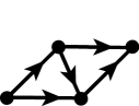
Figure 1: The rhombus graph $H$.

The rhombus directed graph $H$, is defined to be the graph satisfying $V_{H}=\{v_{0},v_{1},v_{2},v_{3}\}$ and $E_{H}=\{v_{0}v_{1},v_{0}v_{2},v_{2}v_{3},v_{1}v_{3},v_{2}v_{1}\}$. We call $v_{0}$ the base vertex of $H$.

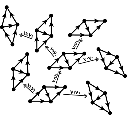
Figure 2: A portion of $H^{*}$, including the names of the vertices of the node $H^{*}_{\text{root}}$ and the labels on the arcs.

We further define $H^{*}$ to be the infinite directed trinary tree whose nodes are copies of $H$, labeling the three arcs emanating from every node by $v_{0}v_{2}$, $v_{2}v_{3}$ and $v_{1}v_{3}$. We write $L(a)$ for the label of an arc $a$. Let $N$ be a node of $H^{*}$, and let $v_{i}v_{j}\in E_{H}$; we call a pair $(N,v_{i})$ a vertex of $H^{*}$, and a pair $(N,v_{i}v_{j})$, an edge of $H^{*}$. Notice the distinction between arcs of $H^{*}$ and edges of $H^{*}$, and the distinction between nodes and vertices. The root of $H^{*}$ is denoted by $H^{*}_{\text{root}}$. A portion of $H^{*}$ is depicted in figure 2.

There exists a natural map $\pi$ from the vertices of $H^{*}$ to the vertices of $T^{*}$ which maps each node of $H^{*}$ to a pair of adjacent triangles of $T^{*}$. $\pi$ is defined in such a way that $H^{*}_{\text{root}}$ is mapped to ${T^{*}_{\text{root}}}$ and to one of its neighboring triangles, and every directed arc $MN$ of $H^{*}$, satisfies $\pi((M,L(MN)))=\pi((N,v_{0}v_{1}))$ (in the sense of mapping origin to origin and destination to destination). In the rest of the paper we extend $\pi$ naturally to edges and subgraphs, and abridge $\pi((N,v))$ to $\pi(N,v)$. A portion of $T^{*}$ and its covering by $H^{*}$ through $\pi$ are depicted in figure 3.

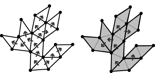
Figure 3: A portion of $T^{*}$ and the corresponding covering by $H^{*}$. The orientation of the edges is omitted to simplify the drawing. The nodes $M$ and $N$ are QR-encoded by $S_{M}=(v_{0}v_{2},v_{2}v_{3},v_{0}v_{2},v_{0}v_{2})$, $\text{QR}(M)=((0,1,0,0),(0,0,0),3)$ and $S_{N}=(v_{0}v_{2},v_{2}v_{3},v_{2}v_{3})$, $\text{QR}(N)=((0,2),(0),1)$ respectively.

Encoding the rhombi. In order to embed $T^{*}$ into $\mathbb{C}$, rhombus-by-rhombus, a way to refer to every node $N\in H^{*}$ is called for. We encode $N$ by the sequence of labels on the path from $H^{*}_{\text{root}}$ to $N$. This trinary sequence is denoted by $S_{N}$. The map $N\to S_{N}$ is a bijection.

One may think of each label in $S_{N}$ as a direction, ”left”, ”right” or ”forward”, in which one must descend $H^{*}$, until finally arriving at $N$. To simplify our proofs, we further encode $S_{N}$, by describing this sequence by ”how many forward steps to take between each turn left or right” and ”is the $i$-th turn left or right”.

Formally, we do this by further encoding $S_{N}$ using a triple $(\{q_{i}(N)\}_{i=1}^{m(N)+1},\{\rho_{i}(N)\}_{i=1}^{m(N)},m(N))$. We set $q_{i}(N)$ to be the number of $v_{2}v_{3}$-s between the $(i-1)$-th non-$v_{2}v_{3}$ label in $S_{N}$ and the $i$-th one (for $i=1$ and for $i=m(N)+1$, the number of $v_{2}v_{3}$-s before the first non-$v_{2}v_{3}$ label in $S_{N}$ and after the last non-$v_{2}v_{3}$ label in $S_{N}$, respectively). We set $\rho_{i}(N)$ to be $0$ if the $i$-th non-$v_{2}v_{3}$ element is $v_{0}v_{2}$ and $1$ if it is $v_{1}v_{3}$. We call the triple $(\{q_{i}(N)\},\{\rho_{i}(N)\},m(N))$ the QR-encoding of $N$ denoting it by $\text{QR}(N)$.

In accordance with our informal introduction, a QR-encoding $(\{q_{i}\},\{\rho_{i}\},m)$, should be interpreted as taking $q_{1}$ steps forward, then turning left or right according to $\rho_{1}$ being $0$ or $1$ respectively, then taking another $q_{2}$ steps forward in the new direction and so on and so forth. The QR-encoding of each node is unique.

Encoding the vertices of $T^{*}$. The encoding of the nodes of $H^{*}$ naturally extends to an encoding of the vertices of $T^{*}$ by defining $\text{QR}(u)=\{\text{QR}(N)\ :\ \pi(N,v_{0})=u\}$ for $u\in T^{*}$. This is indeed an encoding of all the vertices of $T^{*}$, as for every vertex $u\in T^{*}$ there exists at least one node $N$ such that $\pi(N,v_{0})=u$. However, it is not unique, as an infinite number of nodes encode each vertex. As a unique encoding of every vertex is desirable for our purpose, we make the following observation.

Observation 1.

Let $u\in T^{*}$, there exists a unique node $N$ such that $\text{QR}(N)=(\{q_{i}\},\{\rho_{i}\},m)\in\text{QR}(u)$, satisfying $q_{m+1}=0$ and either $q_{m}>0$ or $m=1$. We call such an encoding the proper encoding of $u$.

Proof.

It is not difficult to observe that the only proper encodings of $\pi(H^{*}_{\text{root}},v_{0})$ and $\pi(H^{*}_{\text{root}},v_{1})$ are $((0,0),(0),1)$ and $((0,0),(1),1)$ respectively.

For every vertex $u\in T^{*}$, except from $\pi(H^{*}_{\text{root}},v_{0})$ and $\pi(H^{*}_{\text{root}},v_{1})$, there exists a unique node $N_{u}\in H^{*}$ satisfying that $\pi(N_{u},v_{i})=u$ for some $i\in\{2,3\}$. Let $\sim$ denote the concatenation operation between sequences. Using this notation we have that either $S(N_{u})\sim v_{2}v_{3}\sim v_{0}v_{2}$ or $S(N_{u})\sim v_{2}v_{3}\sim v_{1}v_{3}$ encode a node whose base vertex is mapped by $\pi$ to $u$. One may verify from the definition of QR-encodings that $S_{N}$ ending with either $v_{2}v_{3},v_{0}v_{2}$ or with $v_{2}v_{3}\sim v_{1}v_{3}$ is equivalent to $q_{m+1}=0$ and $q_{m}>0$. ∎

Polynomial embeddings. A $d$-polynomial embedding of a graph $G$ using $k$ edge-lengths is a one-to-one mapping $\psi:V_{G}\to\mathbb{C}[x_{1},\dots,x_{d}]$ where $\mathbb{C}[x_{1},\dots,x_{d}]$ is the space of complex polynomials in $d$ variables, such that for every fixed $x\in\mathbb{T}^{d}=\{(x_{1},\dots,x_{d})\in\mathbb{C}^{d}:\forall i\in\{1,\dots,d\},|x_{i}|=1\}$ the map $v\mapsto\psi(v)(x)=\psi_{x}(v)$ is a linear embedding using only $k$ non-zero edge-lengths.

The importance of $d$-polynomial embeddings to our purpose stems from the following proposition:

Proposition 2.

If $\psi$ is a $d$-polynomial embedding of a graph $G$ with $k$ edge-lengths, then for almost every $x=(x_{1},\dots,x_{d})\in\mathbb{T}^{d}$, $\psi_{x}$ is a degenerate drawing of $G$ with $k$ edge-lengths.

Proof.

For any $v,w\in V_{G}$, the polynomials $\psi(v)(x)$ and $\psi(w)(x)$ may coincide only on a set of measure $0$ in $T^{d}$. Taking union over all the pairs $v_{1},v_{2}$, we get that outside an exceptional set of measure zero in $\mathbb{T}^{d}$, the map $\psi_{x}$ is one-to-one. ∎

4 Three Distances Suffice for Degenerate Drawings

In this section we prove Proposition 1 and thus Theorem 1. To do so, for $x_{0},x_{1}\in\mathbb{T}$, we introduce in section 4.1 a $2$-polynomial embedding $\psi=\psi(x_{0},x_{1})=\psi_{(x_{0},x_{1})}:T^{*}\to\mathbb{C}$. In section 4.2 we then write an explicit formula for the image of every vertex $v$ under $\psi$. This we do using the QR-encoding introduced in the preliminaries section. In section 4.3 we prove that $\psi$ is one-to-one. Finally, in section 4.4 we conclude the proof of Proposition 1.

4.1 The definition of $\psi$

In this section we define $\psi$. An outline of our construction is as follows: we start by presenting $\psi_{H}(x)$, a $1$-polynomial embedding of $H$ which embeds the rhombus graph onto a rhombus of side length $1$ with angle $x$ (identifying the complex number $x$ with its angle on the unit circle). We then use a boolean function Ty on the nodes of $T^{*}$ to decide whether each rhombus is mapped to a translated and rotated copy of $H(x_{0})$ or of $H(x_{1})$. Finally, we define $\psi$ in the only way that respects both the covering $\pi$ and the function Ty. The image of several subsets of $T^{*}$ through $\psi(x_{0},x_{1})$ is depicted in figure 5.

We set $\psi_{H}(x)(v_{0})=0$, $\psi_{H}(x)(v_{1})=1$, $\psi_{H}(x)(v_{2})=x$ and $\psi_{H}(x)(v_{3})=x+1$. This is indeed a polynomial drawing, mapping the rhombus graph to a rhombus of edge length $1$, whose $v_{1}v_{0}v_{2}$ angle is $x$. Figure 4 illustrates the image of $H$ under $\psi_{H}$.

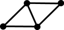
Figure 4: The image of $H$ under $\psi_{H}$. Observe how $x$ determines the $v_{1}v_{0}v_{2}$ angle of the rhombus.

We define an auxiliary function Ty. Let $MN$ be an arc of $H^{*}$. We set

$$\text{Ty}(N)=\begin{cases}\text{Ty}(M)&L(MN)=v_{2}v_{3}\\ \text{Ty}(N)\oplus q_{m(M)+1}(M)\pmod{2}&L(MN)=v_{0}v_{2}\\ \text{Ty}(N)\oplus q_{m(M)+1}(M)\oplus 1\pmod{2}&L(MN)=v_{1}v_{3}\\ \end{cases},$$ (1)

where $\oplus$ represents addition modulo $2$. We set $\text{Ty}(H^{*}_{\text{root}})=0$.

Set $\psi(\pi(H^{*}_{\text{root}}))=\psi_{H}(x_{0})(H)$. Let $M,N\in H^{*}$ be a pair of nodes such that $MN$ is an arc of $H^{*}$, and assume that $\psi$ is already defined on the vertices of $\pi(M)$. By $\pi$’s definition, this implies that $\psi(\pi(N,v_{0}))$ and $\psi(\pi(N,v_{1}))$ are already defined. We then define $\psi(\pi(N,v_{2})),\psi(\pi(N,v_{3}))$ so that $\psi(\pi(N,v_{0})),\psi(\pi(N,v_{1})),\psi(\pi(N,v_{2})),\psi(\pi(N,v_{3}))$ form a translated and rotated copy of $H(x_{\text{Ty}(N)})$.

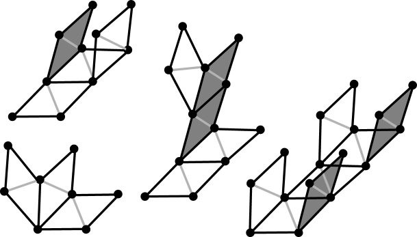
Figure 5: The image of several subgraphs of $T^{*}$ under $\psi$. Explicit values are given for several vertices. In each graph, the image of $\pi(H^{*}_{\text{root}})$ under $\psi$ is marked by $R$. Rhombi of angle $x_{1}$ are dark.

As the image of every edge in $T^{*}$ is isometric to some edge of either $H(x_{0})$ or $H(x_{1})$, we get

Observation 2.

Every edge of $T^{*}$ is mapped through $\psi$ to an interval of length $1$, $|x_{0}-1|$, or $|x_{1}-1|$.

While this definition of $\psi(x_{0},x_{1})$ is complete, an explicit formula for every vertex in $T^{*}$ under $\psi(x_{0},x_{1})$ is required for proving that $\psi$ is indeed a polynomial embedding. We devote the next section to develop this formula.

4.2 The image of $\psi$

In this section we state a formula for $\psi\circ\pi$ of every base vertex.

Let $u\in T^{*}$ and let $N\in H^{*}$, such that $\text{QR}(N)=(\{q_{k}\},\{\rho_{k}\},m)$ is the proper encoding of $u$. The first $i$ elements of $\{q_{k}\},\{\rho_{k}\}$ encode a node in $T^{*}$ which is denoted by $N_{i}$ (where $N_{0}=H^{*}_{\text{root}}$ which corresponds to the null sequence). Naturally, $N_{m}=N$. From (1) we get

$$\text{Ty}(N_{i})=\text{Ty}(N_{i-1})\oplus q_{i}\oplus\rho_{i}\pmod{2}.$$ (2)

Observe that in the embedding of every $H^{*}$ node through $\psi$, the edges $v_{0}v_{2}$, $v_{1}v_{3}$ are parallel, as are the edges $v_{0}v_{1},v_{2}v_{3}$. Next, we define $P_{i}(x_{0},x_{1})$ to be a unit vector in the direction of the edges $(v_{0},v_{1}),(v_{2},v_{3})$ in $\psi(\pi(N_{i}))$ which, for $i>0$, is the same as the direction of $(v_{0},v_{2}),(v_{1},v_{3})$ in $\psi(\pi(N_{i-1}))$.

Formally

$$P^{u}_{i}(x_{0},x_{1})=P_{i}(x_{0},x_{1})=\psi(\pi(N_{i},v_{1}))-\psi(\pi(N_{i},v_{0}))=\psi(\pi(N_{i-1},v_{2})-\psi(\pi(N_{i-1},v_{0})),$$

where the last equality holds for $i>0$. Notice that $P_{0}(x_{0},x_{1})=1$.

With this in mind, it is possible to follow the change in $P_{i}$ between one $N_{i}$ and the next. This yields:

$$P_{i}(x_{0},x_{1})=P_{i-1}(x_{0},x_{1})\cdot x_{\text{Ty}(N_{i-1})}.$$ (3)

For $0\leq i\leq m$ write $Q^{u}_{i}(x_{0},x_{1})=Q_{i}(x_{0},x_{1})=\psi_{x_{0},x_{1}}(\pi(N_{i},v_{0}))$. Observe that $Q_{0}=\psi(\pi(H^{*}_{\text{root}},v_{0}))=0$. Let us describe how to get $Q_{i}$ from $Q_{i-1}$ using $(\{q_{k}\},\{\rho_{k}\},m)$. By definition,

$$Q_{i}(x_{0},x_{1})-Q_{i-1}(x_{0},x_{1})=\psi(\pi(N_{i},v_{0}))-\psi(\pi(N_{i-1},v_{0})).$$

Thus $Q_{i}(x_{0},x_{1})-Q_{i-1}(x_{0},x_{1})$ can be calculated from the labels of the edges along the path connecting $(N_{i-1},v_{0})$ and $(N_{i},v_{0})$. Each edge labeled $v_{2}v_{3}$ contributes to this difference $P_{i}$, and thus in total such edge contribute $q_{i}\cdot P_{i}$. An edge with label $v_{1}v_{3}$ contributes $P_{i}/{x_{\text{Ty}(N_{i-1})}}=P_{i-1}$, while an edge labeled $v_{0}v_{2}$ does not change the base vertex at all.

Applying this to the encoding, we get that

$$Q_{i}-Q_{i-1}=q_{i}\cdot P_{i}+\rho_{i}\cdot P_{i-1}.$$

Summing this over $1\leq i\leq m$, we get:

$$\psi_{x_{0},x_{1}}(u)=Q_{m} =\sum_{i=1}^{m}\left(q_{i}P_{i}+\rho_{i}P_{i-1}\right)$$

$$=\rho_{1}+\sum_{i=1}^{m-1}\left(q_{i}+\rho_{i+1}\right)P_{i}+q_{m}P_{m}$$

Equivalently, letting $\rho_{m}=0$ and $q_{0}=0$ we have

$$\psi_{x_{0},x_{1}}(u)=\sum_{i=0}^{m}\left(q_{i}+\rho_{i+1}\right)P_{i}(x_{0},x_{1})=\sum_{i=0}^{m}c_{i}P_{i}(x_{0},x_{1}),$$ (4)

where

$$c_{i}=q_{i}+\rho_{i+1}.$$ (5)

Observe that for every $u\in T^{*}$, $\psi_{x_{0},x_{1}}(u)$ is a polynomial in $x_{0}$ and $x_{1}$ (because $P_{i}$ are monomials). Also observe that the total degree of $P_{i}$, which we denote by $\text{deg}P_{i}$, obeys $\text{deg}P_{i}=\text{deg}P_{i-1}+1$. Therefore $\{c_{i}\}$ may be regarded as the coefficients of the polynomial $\psi_{x_{0},x_{1}}(u)$.

Note that in particular, using the above notations, Observation 1 and the fact that $(\{q_{k}\},\{\rho_{k}\},m)$ is proper yield

$$c_{m}=q_{m}>0.$$ (6)

4.3 Showing that $\psi$ is a polynomial embedding

In this section we show that the image of the vertices of $T^{*}$ under $\psi$ are all distinct. Relation (4) and Observation 2 imply that if this is the case, then $\psi$ is a polynomial embedding of $T^{*}$ using three edge lengths.

The main proposition of this section is the following:

Proposition 3.

Let $u,w\in T^{*}$ be two distinct vertices. Then $\psi_{x_{0},x_{1}}(u)$ and $\psi_{x_{0},x_{1}}(w)$ are distinct polynomials.

Proof.

Let $(\{q^{u}_{i}\},\{\rho^{u}_{i}\},m)$,$(\{q^{w}_{i}\},\{\rho^{w}_{i}\},n)$ be the proper QR-encoding sequences for $u,w$ respectfully, and let $N_{k}^{u}$ and $N_{k}^{w}$ be the nodes encoded by the first $k$ elements of those sequences respectively. We write $\nu^{u}_{i}=\text{Ty}(N_{i}^{u})$, $\nu^{w}_{i}=\text{Ty}(N_{i}^{w})$ for all $i$.

Notice that by Observation 1 the two sequences are distinct. The fact that $\pi(H^{*}_{\text{root}},v_{0})$ and $\pi(H^{*}_{\text{root}},v_{1})$ have unique images under $\psi$ is straightforward, as these are the only vertices whose image is a polynomial of total degree $0$. We can therefore assume $m>1$.

Assume for the sake of obtaining a contradiction that $\psi_{x_{0},x_{1}}(u)\equiv\psi_{x_{0},x_{1}}(w)$ as functions of $(x_{0},x_{1})$, and thus in particular $c^{u}_{i}=c^{w}_{i}$ for all $i$.

Combining this with (6) and Observation 1, we get $m=n$.

Let $j$ be the first index to satisfy $(q^{u}_{j},\rho^{u}_{j})\neq(q^{w}_{j},\rho^{w}_{j})$. By (2) and (3) this implies

$$\forall i\leq j:P^{u}_{i}=P^{w}_{i}\text{ and }\nu^{u}_{i-1}=\nu^{w}_{i-1}.$$ (7)

Moreover, since $q^{u}_{j-1}=q^{w}_{j-1}$ and $c^{u}_{j-1}=c^{w}_{j-1}$ we get by (5) that $\rho^{u}_{j}=\rho^{w}_{j}$. We deduce that $q^{u}_{j}\neq q^{w}_{j}$. Since $c^{u}_{j}=c^{w}_{j}$ we have $q^{u}_{j}-q^{w}_{j}=\rho^{w}_{j+1}-\rho^{u}_{j+1}\in\{-1,0,1\}$. As we have assumed this difference to be non-zero, we may assume without loss of generality

$$q^{u}_{j}-q^{w}_{j}=\rho^{w}_{j+1}-\rho^{u}_{j+1}=1.$$ (8)

Applying (7) for $i=j+1$ and the last relation to (2), we get

$$\nu^{u}_{j}=\nu^{u}_{j-1}\oplus q^{u}_{j}\oplus\rho^{u}_{j}=\nu_{j-1}^{w}\oplus q^{w}_{j}\oplus\rho^{w}_{j}\oplus 1=\nu_{j}^{w}\oplus 1.$$

By (3) we get

$$\frac{P^{u}_{j+1}}{P^{w}_{j+1}}=\frac{x_{\nu^{u}_{j}}}{x_{\nu^{w}_{j}}}\neq 1,$$

which implies $c^{u}_{j+1}=c^{w}_{j+1}=0$. This in turn implies that $q^{u}_{j+1}=q^{w}_{j+1}=0$ and $\rho^{u}_{j+2}=\rho^{w}_{j+2}=0$. Using now relation (2) for $i=j+2$ and recalling (8), we get

$$\nu^{u}_{j+2}=\nu^{u}_{j+1}\oplus 0\oplus\rho^{u}_{j+1}=(\nu^{w}_{j+1}\oplus 1)\oplus 0\oplus(\rho^{w}_{j+1}-1)=\nu^{w}_{j+2}.$$

Again by (3) we have

$$\frac{P^{u}_{j+2}}{P^{w}_{j+2}}=\frac{P^{u}_{j+1}}{P^{w}_{j+1}}\cdot\frac{x_{\nu^{u}_{j+2}}}{x_{\nu^{w}_{j+2}}}=\frac{P^{u}_{j+1}}{P^{w}_{j+1}}\neq 1,$$

which implies $c^{u}_{j+2}=c^{w}_{j+2}=0$. Continuing by induction, we conclude that $c^{u}_{j+k}=c^{w}_{j+k}=0$ for all $k>1$. Thus $j=m$, and so by (6), $q^{u}_{j}=c^{u}_{j}=c^{w}_{j}=q^{w}_{j}$, a contradiction to (8). ∎

4.4 Three Distances Suffice for Degenerate Drawings

We are now ready to present the proof of Proposition 1, and thus conclude the proof of Theorem 1.

Proof of Proposition 1.

By Proposition 3, $\psi$ is a $2$-polynomial embedding of every finite subgraph $G\subseteq T^{*}$, using $3$ edge-lengths. By Proposition 2 and Observation 2, the set

$$\{(x_{0},x_{1})\ :\ \text{s.t. }x_{0},x_{1}\in\mathbb{T}^{2}\text{ and }\psi(x_{0},x_{1})\text{ is a degenerate drawing}\}$$

is of full measure, and each of these degenerate drawings uses only side lengths $1$, $|x_{0}-1|$ and $|x_{1}-1|$. Let $a\in(0,1)$, the embedding $a\cdot\psi$, i.e. the composition of a multiplication by $a$ on $\psi$, is thus a degenerate drawing of $G$ for almost every $x_{0},x_{1}$ using the side lengths $a,a|1-x_{0}|,a|1-x_{1}|$. The desired result follows. ∎

4.5 Open problems

Several interesting problems concerning graphs with a low (degenerate) distance number remain open. In this short section we state those of greater interest to us. The first and most natural one is:

Problem 1.

Do outerplanar graphs have a uniformly bounded distance number?

While we believe we may be able to answer this problem positively, our construction is rather complicated and is thus postponed to a future paper. It will be interesting to see a simple construction which can be easily described.

The general problem which, in our opinion, extends this work most naturally is:

Problem 2.

Which families of graphs have a uniformly bounded (degenerate) distance number?

Observe that the family of planar graphs does not have this property, as the complete bipartite graph $K_{2,n}$ is an example of a planar graph whose degenerate distance number is $\Theta(\sqrt{n})$.

Finally, our result implies that the maximum possible degenerate distance number of an outerplanar graph is at most three. It is easy to see that there are outerplanar graphs whose degenerate distance number is two. Are there any outerplanar graphs whose degenerate distance number is indeed three?

Problem 3.

Is it true that the maximum possible degenerate distance number of an outerplanar graph is two?

References

- [1] P. Carmi, V. Dujmovic, P. Morin and D. Wood. Distinct distances in graph drawings (2008). Electronic Journal of Combinatorics 15:1.
- [2] P. Erdős. On sets of distances of n points(1946). Amer. Math. Monthly, 53:248–250.
- [3] L. Guth and N H. Katz. On the Erdős distinct distance problem in the plane (2010). arXiv:1011.4105v3 [math.CO]
- [4] N. H. Katz and G. Tardos. A new entropy inequality for the Erdős distance problem. Towards a theory of geometric graphs, vol. 342 of Contemp. Math., pp. 119–126. Amer. Math. Soc., 2004.
- [5] J. Pach and P K. Agarwal. Combinatorial Geometry. John Wiley & Sons Inc., 1995, New York.
- [6] J. H. Spencer, E. Szemerédi and W T. Trotter Jr. Unit distances in the Euclidean plane. In B. Bollobás, ed., Graph theory and combinatorics, pp. 293–303. Academic Press, 1984, London.
- [7] L A. Székely. Crossing numbers and hard Erdős problems in discrete geometry. Combin. Probab. Comput.(1997), 6(3):353–358.