¹³CO and C¹⁸O $J=2-1$ mapping of the environment of the Class 0 protostellar core SMM 3 in Orion B9

Abstract

Context. Observations of molecular spectral lines provide information on the gas kinematics and chemistry of star-forming regions.

Aims. We attempt to achieve a better understanding of the gas distribution and velocity field around the deeply embedded Class 0 protostar SMM 3 in the Orion B9 star-forming region.

Methods. Using the APEX 12-m telescope, we mapped the line emission from the $J=2-1$ rotational transition of two CO isotopologues, ¹³CO and C¹⁸O, over a $4\arcmin\times 4\arcmin$ region around Orion B9/SMM 3.

Results. Both the ¹³CO and C¹⁸O lines exhibit two well separated velocity components at about 1.3 and 8.7 km s^-1. The emission of both CO isotopologues is more widely distributed than the submillimetre dust continuum emission as probed by LABOCA. The LABOCA 870-$\mu$m peak position of SMM 3 is devoid of strong CO isotopologue emission, which is consistent with our earlier detection of strong CO depletion in the source. No signatures of a large-scale outflow were found towards SMM 3. The ¹³CO and C¹⁸O emission seen at $\sim 1.3$ km s^-1 is concentrated into a single clump-like feature at the eastern part of the map. The peak H₂ column density towards a C¹⁸O maximum of the low-velocity component is estimated to be $\sim 10^{22}$ cm^-2. A velocity gradient was found across both the ¹³CO and C¹⁸O maps. Interestingly, SMM 3 lies on the border of this velocity gradient.

Conclusions. The ¹³CO and C¹⁸O emission at $\sim 1.3$ km s^-1 is likely to originate from the “low-velocity part” of Orion B. Our analysis suggests that it contains high density gas ($\sim 10^{22}$ H₂ molecules per cm²), which conforms to our earlier detection of deuterated species at similarly low radial velocities. Higher-resolution observations would be needed to clarify the outflow activity of SMM 3. The sharp velocity gradient in the region might represent a shock front resulting from the feedback from the nearby expanding H ii region NGC 2024. The formation of SMM 3, and possibly of the other members of Orion B9, might have been triggered by this feedback.

1 Introduction

The protostellar phase of low-mass star formation begins when a starless (prestellar) core collapses, and, after a hypothesised short-lived first-hydrostatic core stage (Larson (1969); Masunaga et al. (1998)), a stellar embryo forms in its centre (the so-called second hydrostatic core; e.g., Masunaga & Inutsuka (2000)). The dense cores harbouring the youngest protostars are known as the Class 0 objects (André et al. (1993), 2000). In these objects, most of the system’s mass resides in the dense envelope, i.e., $M_{\rm env}\gg M_{\star}$, where $M_{\star}$ is the mass of the central protostar. For this reason, Class 0 objects, or at least the youngest of them, are expected to still represent the initial physical conditions prevailing at the time of collapse phase. Class 0 objects are characterised by accretion-powered jets and molecular outflows, which can be very powerful and highly collimated (e.g., Bontemps et al. (1996); Gueth & Guilloteau (1999); Arce & Sargent (2005), 2006; Lee et al. (2007)). The statistical lifetime of the Class 0 stage is estimated to be $\sim 1\times 10^{5}$ yr (Evans et al. (2009); Enoch et al. (2009)), but the exact duration of this embedded phase of evolution can be highly dependent on the initial/environmental conditions (e.g., Vorobyov (2010)).

The target source of the present study is the Class 0 protostellar core SMM 3 in the Orion B9 star-forming region, which was originally discovered by Miettinen et al. (2009; Paper I) through LABOCA 870-$\mu$m dust continuum mapping of the region. SMM 3 is a strong submm emitting dust core ($S_{870}\simeq 2.5$ Jy) that is associated with a weak Spitzer 24-$\mu$m point source ($S_{24}\simeq 5$ mJy), and a 3.6 Jy point source at 70 $\mu$m. Using the Effelsberg 100-m telescope NH₃ observations, Miettinen et al. (2010; Paper II) derived the gas kinetic temperature of $T_{\rm kin}=11.3\pm 0.8$ K in SMM 3. Using this temperature, the core mass was determined to be $7.8\pm 1.6$ M_☉, and its volume-averaged H₂ number density was estimated to be $1.1\pm 0.2\times 10^{5}$ cm^-3. In the SABOCA 350-$\mu$m mapping of Orion B9 by Miettinen et al. (2012; Paper III), SMM 3 was found to be by far the strongest source in the mapped area ($S_{350}\simeq 5.4$ Jy). We also found that it contains two subfragments, or condensations (we called SMM 3b and 3c), lying about $36\arcsec-51\arcsec$ in projection from the central protostar. These correspond to 0.08–0.11 pc or $\sim 1.7-2.3\times 10^{4}$ AU at $d=450$ pc. Because the thermal Jeans length of the core is $\lambda_{\rm J}=0.07$ pc, we suggested that the core fragmentation into condensations can be explained by thermal Jeans instability. Using the 350/870-$\mu$m flux density ratio, we determined the dust temperature of the core to be $T_{\rm dust}=10.8_{-2.6}^{+5.7}$ K, which is very close to $T_{\rm kin}$ within the error bars. The revised spectral energy distribution (SED) of the core yielded a very low dust temperature of 8 K, and a bolometric luminosity of $L_{\rm bol}=1.2\pm 0.1$ L_☉. The latter is very close to the median luminosity of protostars in nearby star-forming regions, i.e., $L_{\rm med}=1.5^{+0.7}_{-0.4}$ L_☉ (Enoch et al. (2009); Offner & McKee (2011)). In Paper III, we also studied the chemistry of SMM 3. We derived a large CO depletion factor of $f_{\rm D}({\rm CO})=10.8\pm 2.2$, and a high level of deuterium fractionation, i.e., a ${\rm N_{2}D^{+}}/{\rm N_{2}H^{+}}$ column density ratio of $0.338\pm 0.092$. In Fig. 1, we show the LABOCA 870-$\mu$m, SABOCA 350-$\mu$m, and Spitzer 4.5/24-$\mu$m images towards SMM 3. In Table 1, we provide an overview of the physical and chemical properties of SMM 3 derived in our previous papers.

In this paper, we discuss the results of our ¹³CO and C¹⁸O mapping observations of the environment of SMM 3. We analyse the structure of the mapped region as traced by emission from the $J=2-1$ rotational transition of the above CO isotopologues. The rest of the present paper is organised as follows. Observations and data reduction are described in Sect. 2. Mapping results and analysis are presented in Sect. 3. In Sect. 4, we discuss our results, and in Sect. 5, we summarise and conclude the paper.

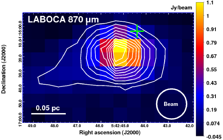
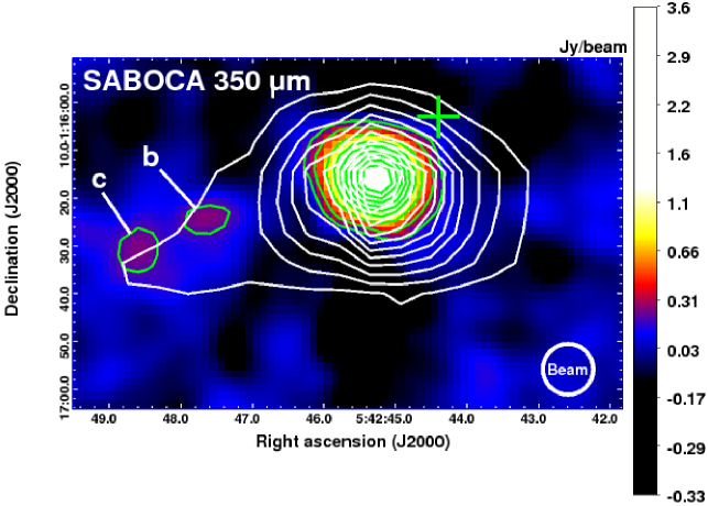
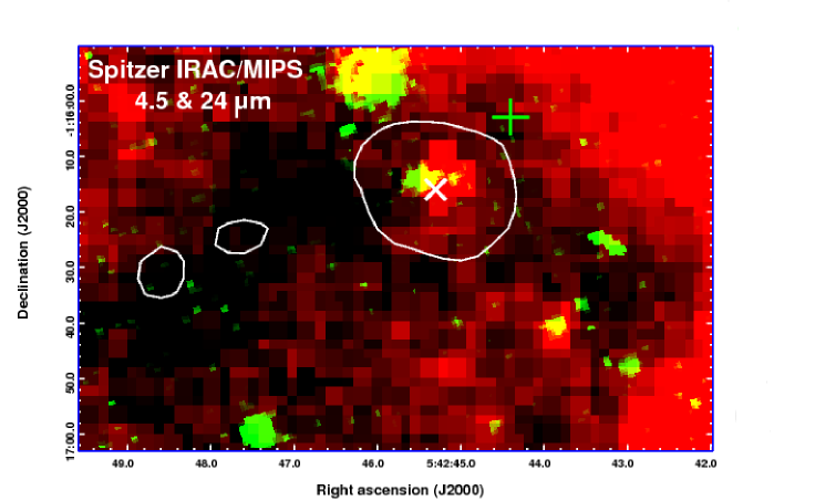
Figure 1: LABOCA 870-$\mu$m (top), SABOCA 350-$\mu$m (middle), and a Spitzer IRAC/MIPS two-colour composite image (bottom; 4.5 $\mu$m in green and 24 $\mu$m in red) of the Class 0 protostellar core SMM 3 in Orion B9. The LABOCA and Spitzer images are shown with linear scaling, while the SABOCA image is shown with a square-root scaling to improve the contrast between bright and faint features. The LABOCA contours, plotted in white, go from 0.1 ($\sim 3.3\sigma$) to 1.0 Jy beam^-1 in steps of 0.1 Jy beam^-1. The SABOCA contour levels, plotted in green, start at $3\sigma$ and are 0.18 Jy beam${}^{-1}\times[1,\,2,\,4,\,6,\,8,\,10,\,12,\,14,\,16]$. In the bottom panel, the first SABOCA contour, i.e., the $3\sigma$ emission level, is plotted in white to guide the eye, and the white cross indicates the SABOCA peak position of SMM 3. The small subcondensations SMM 3b and 3c discovered in Paper III are labeled in the middle panel. The green plus sign shows the target position of our previous molecular-line observations (i.e., the submm peak position of the LABOCA map before adjusting the pointing; see Paper III for details). A scale bar indicating the 0.05 pc projected length is shown in the bottom left of the top panel, with the assumption of a 450 pc line-of-sight distance. The effective LABOCA and SABOCA beams, $\sim 20\arcsec$ and $10\aas@@fstack{\prime\prime}6$, are shown in the lower right corners of the corresponding panels.

Table 1: Summary of the properties of SMM 3.

Parameter	Value
SMM 3
$\alpha_{2000.0}$	05h 42m $45\aas@@fstack{s}3$
$\delta_{2000.0}$	-01°16′16″
${\rm v}_{\rm LSR}$	$8.68\pm 0.06$ km s-1
$R_{\rm eff}$	13$\aas@@fstack{\prime\prime}$3 (0.03 pc)
$T_{\rm kin}$	$11.3\pm 0.8$ K
$T_{\rm dust}$	$10.8_{-2.6}^{+5.7}$ K
$T_{\rm dust}^{\rm SED,\,cold}$	8.0 K
$\sigma_{\rm NT}$	$0.14\pm 0.003$ km s-1
$\sigma_{\rm NT}/c_{\rm s}$	$0.7\pm 0.04$
$M$	$7.8\pm 1.6$ M☉/$2.1\pm 0.8$ M☉
$\alpha_{\rm vir}$	$0.5\pm 0.1$
$N({\rm H_{2}})$	$8.4\pm 1.1\times 10^{22}$/$1.0\pm 0.3\times 10^{23}$ cm-2
$\langle n({\rm H_{2}})\rangle$	$1.1\pm 0.2\times 10^{5}$/$4.0\pm 1.5\times 10^{5}$ cm-3
$L_{\rm bol}=L_{\rm cold}+L_{\rm warm}$	$(0.3\pm 0.1)+(0.9\pm 0.1)=1.2\pm 0.1$ L☉
$L_{\rm submm}/L_{\rm bol}$	0.1
$f_{\rm D}({\rm CO})$	$10.8\pm 2.2$
$[{\rm N_{2}D^{+}}]/[{\rm N_{2}H^{+}}]$	$0.338\pm 0.092$
SMM 3b
$\alpha_{2000.0}$	05h 42m $47\aas@@fstack{s}6$
$\delta_{2000.0}$	-01°16′24″
$N({\rm H_{2}})$	$0.7\pm 0.2\times 10^{22}$ cm-2
SMM 3c
$\alpha_{2000.0}$	05h 42m $48\aas@@fstack{s}6$
$\delta_{2000.0}$	-01°16′32″
$N({\rm H_{2}})$	$0.7\pm 0.2\times 10^{22}$ cm-2

2 Observations and data reduction

The observations presented in this paper were made on 13 November 2011 using the APEX 12-m telescope located at Llano de Chajnantor in the Atacama desert of Chile. The telescope and its performance are described in the paper by Güsten et al. (2006). An area of $4\arcmin\times 4\arcmin$ (0.52 pc $\times$ 0.52 pc at $d=450$ pc) was simultaneously mapped in the $J=2-1$ rotational lines of ¹³CO and C¹⁸O using the total power on-the-fly mode towards SMM 3 centred on the coordinates $\alpha_{2000.0}=05^{\rm h}42^{\rm m}45\aas@@fstack{s}8$, $\delta_{2000.0}=-01\degr 16\arcmin 13\aas@@fstack{\prime\prime}0$ [$(+7\aas@@fstack{\prime\prime}5,\,+3\aas@@fstack{\prime\prime}0)$ offset from the SABOCA peak position of SMM3]. At the ¹³CO$(2-1)$ and C¹⁸O$(2-1)$ line frequencies, 220 398.70056 and 219 560.357 MHz, respectively, the telescope beam size is about $28\aas@@fstack{\prime\prime}3$ (HPBW). The target area was scanned alternately in right ascension and declination, i.e., in zigzags to ensure minimal striping artefacts in the final data cubes. Both the stepsize between the subscans and the angular separation between two successive dumps was $9\aas@@fstack{\prime\prime}4$, i.e., about 1/3 times the beam HPBW ensuring Nyquist sampling. We note that the readout spacing $1/3\times{\rm HPBW}$ should not be exceeded to avoid beam smearing. The integration time per dump and per pixel was 1 s.

As a frontend, we used the APEX-1 receiver of the Swedish Heterodyne Facility Instrument (SHeFI; Belitsky et al. (2007); Vassilev et al. 2008a ,b). The backend was the RPG eXtended bandwidth Fast Fourier Transfrom Spectrometer (XFFTS; cf. Klein et al. (2012)) with an instantaneous bandwidth of 2.5 GHz and 32 768 spectral channels. The resulting channel separation, 76.3 kHz, corresponds to about 0.1 km s^-1 at 220 GHz.

The telescope pointing accuracy was checked by CO$(2-1)$ cross maps of the variable star RAFGL865 (V1259 Ori), and was found to be consistent within $\lesssim 4\arcsec$. The focus was checked by measurements on Jupiter. Calibration was made by means of the chopper-wheel technique and the output intensity scale given by the system is $T_{\rm A}^{\star}$, which represents the antenna temperature corrected for the atmospheric attenuation. The amount of precipitable water vapour (PWV) was in the range 1.28 – 1.48 mm, and the single-sideband system temperature was around 150 K (in $T_{\rm A}^{\star}$ units). The observed intensities were converted to the main-beam brightness temperature scale by $T_{\rm MB}=T_{\rm A}^{\star}/\eta_{\rm MB}$, where $\eta_{\rm MB}=0.75$ is the main-beam efficiency at the frequencies used. The absolute calibration uncertainty is estimated to be about 10%.

The spectra were reduced and the maps were produced using the CLASS90 and GREG programmes of the GILDAS software package. The individual spectra were Hanning-smoothed to improve the signal-to-noise ratio of the data. A third-order polynomial was applied to correct the baseline in the spectra. The resulting $1\sigma$ rms noise level of the average spectra are about 30 mK (in $T_{\rm MB}$) at the smoothed resolution (16 384 channels). The data were convolved with a Gaussian of 1/3 times the beam HPBW, and therefore the effective angular resolution of the final data cubes is about $30\arcsec$. The average $1\sigma$ rms noise level of the completed maps ranges from 0.20 to 0.28 K per 0.2 km s^-1 channel on a $T_{\rm MB}$ scale. The constructed data cubes were exported in FITS format for further processing in IDL.

3 Mapping results and analysis

3.1 The average spectra

The average ¹³CO$(2-1)$ and C¹⁸O$(2-1)$ spectra are shown in Fig. 2. Both lines exhibit two well-separated velocity components: one near the systemic velocity of about 8.7 km s^-1, and the other at 1.3–1.4 km s^-1. It is not surprising that we see these lower-velocity components in the lines of CO isotopologues. The additional lines at comparable radial velocities of 1.3–1.9 km s^-1 were already detected in the lines of N₂H${}^{+}(1-0)$ and N₂D${}^{+}(2-1)$ in Paper I, NH${}_{3}(1,\,1)$ and $(2,\,2)$ in Paper II, and C¹⁷O$(2-1)$, H¹³CO${}^{+}(4-3)$, DCO${}^{+}(4-3)$, N₂H${}^{+}(3-2)$, and N₂D${}^{+}(3-2)$ in Paper III towards other cores in Orion B9. Therefore, detection of lower-velocity line emission from CO isotopologues was expected. We note that the average ¹³CO line near the systemic velocity of SMM 3 appears to show a blue asymmetric profile with blue peak being stronger than the red peak. The central dip also appears to be near the radial velocity derived from optically thin C¹⁷O$(2-1)$ line in Paper III. Despite of these characteristics, the double-peaked line profile is not caused by infall motions (e.g., Myers et al. (1996)); it results from averaging over the entire mapped area, where two separate velocity components at about 8.5 and 9.5 km s^-1 are seen. This issue will be further discussed in Sect. 3.3. The average C¹⁸O line profile at the systemic velocity is nearly Gaussian, which suggests that the line is likely to be optically thin. However, a hint of the two nearby velocity components is also visible in the average C¹⁸O line; the line exhibits a small “knee” at $\sim 9.5$ km s^-1.

It can also be seen from Fig. 2 that some of the observation OFF positions had ¹³CO emission in the velocity regime between about 2.4 and 4.8 km s^-1, and between about 10.3 and 11.3 km s^-1, and C¹⁸O emission in the range 2.0–3.3 km s^-1. These velocity regimes show up as artificial absorption features in the average spectra. Given the ubiquitous nature of multiple velocity components along the line of sight towards Orion B9, finding an emission free OFF position from this region can be difficult.

The main purpose of examining the average spectra is to determine the velocity range of the detected emission. This is needed to construct the line-emission maps, as will be described in the next section.

Figure 2: Hanning-smoothed spatially averaged ¹³CO$(2-1)$ and C¹⁸O$(2-1)$ spectra across the mapped field. The C¹⁸O$(2-1)$ spectrum is offset by -1.45 K from zero baseline for reasons of clarity. The vertical red dashed line indicates the systemic velocity of SMM 3 derived from C¹⁷O$(2-1)$ in Paper III.

3.2 Moment maps

To display the intensity and kinematic structure of the ¹³CO and C¹⁸O line emission, we constructed the moment maps by integrating the lines over the following LSR velocity ranges: $[6.09,\,10.36]$ km s^-1 and $[7.77,\,10.36]$ km s^-1 for the ¹³CO and C¹⁸O lines of the main velocity component, and $[-0.07,\,2.52]$ km s^-1 and $[0.14,\,2.10]$ km s^-1 for the ¹³CO and C¹⁸O lines of the lower-velocity component (at $\sim 1.3$ km s^-1). These line windows were selected so that the artificial absorption features discussed above are avoided. The threshold used for the moment maps was chosen to be 2 times the rms noise, i.e., $2\sigma$.

The zeroth, first, and second moment maps (i.e., the images of integrated intensity, intensity-weighted central velocity, and intensity-weighted FWHM linewidth) of the ¹³CO and C¹⁸O emission of the main velocity component are shown in Fig. 3, while those of the lower-velocity component are shown in Fig. 4.

The map of ¹³CO integrated intensity (upper left panel of Fig. 3) shows that there is a local emission minimum close to the SMM 3 protostellar position. This conforms to the high level of CO depletion derived from C¹⁷O data. The ¹³CO emission around SMM 3 is rather extended, which is not surprising because it arises from the lower-density gas. In contrast, the LABOCA dust continuum emission shows only the densest part of the region, i.e., SMM 3. The ¹³CO emission appears to be strongest at about $2\arcmin$ south of SMM 3, and from there it extends to the northwest part of the map. From the lower left panel of Fig. 3, it can be seen that the C¹⁸O emission follows quite well the morphology of the ¹³CO emission. There is a hint of an elongated filament-type feature along the NE to the SW direction with relatively strong emission. There appears to be a few C¹⁸O maxima at the eastern part of SMM 3, one lying at the eastern tip of the $3.3\sigma$ LABOCA contour, and the other about $24\arcsec$ from the central protostar.

In the case of the lower-velocity component, both the ¹³CO and C¹⁸O emission are less extended, and are instead concentrated into a single clump-like feature at the eastern part of the mapped region (left panels of Fig. 4). There is a ¹³CO extension to the south of SMM 3 in projection, which is not seen in C¹⁸O.

Interestingly, as can be seen from the first-order moment map of ¹³CO (top middle panel of Fig. 3), there is a fairly sharp border between the two velocity fields, and SMM 3 appears to lie exactly between them, i.e., at the border of the velocity gradient. There is also a hint of increasing ¹³CO linewidth across this border as shown in the top right panel of Fig. 3. The radial-velocity structure of C¹⁸O emission is quite similar to that of ¹³CO, but the C¹⁸O linewidths show less obvious spatial trend (lower middle and right panels of Fig. 3).

Another interesting feature concerning the radial-velocity distribution is that also the lower-velocity component of C¹⁸O shows a somewhat similar gradient across the map (Fig. 4; lower middle panel). Implications of the velocity gradient will be discussed further in Sect. 4.3.

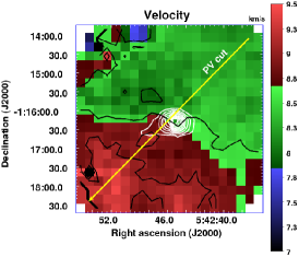
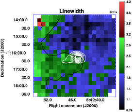
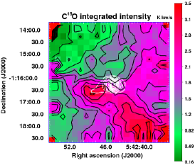
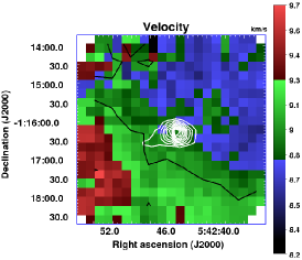
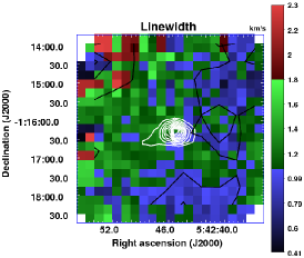
Figure 3: The colour scale in the panels from left to right shows, respectively, the 0th (integrated intensity in $T_{\rm MB}$), 1st (intensity-weighted centroid velocity structure), and 2nd moment (intensity-weighted linewidth structure) map of the 8.7-km s^-1 component ¹³CO$(2-1)$ (top row) and C¹⁸O$(2-1)$ emission (bottom row). The black contours in the upper panels, from left to right, go as follows: from 0.7 ($3.2\sigma$) to 7.0 K km s^-1 ($32\sigma$) in steps of 0.7 K km s^-1; from 7 to 9.5 km s^-1 in steps of 0.5 km s^-1; and from 1 to 4 km s^-1 in steps of 1 km s^-1. The corresponding contours in the lower panels are from 0.4 ($2\sigma$) to 3.2 K km s^-1 ($16\sigma$) in steps of 0.4 K km s^-1; from 7 to 9.5 km s^-1 in steps of 0.5 km s^-1; and from 0.5 to 2 km s^-1 in steps of 0.5 km s^-1. Superimposed on the maps are the LABOCA 870-$\mu$m contours in white as in Fig. 1. The yellow solid line on the top left and middle panels shows the location of the PV slice extracted for Fig. 7. The effective beam size of $30\arcsec$ is shown in the upper left corner of the upper left panel.

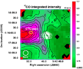
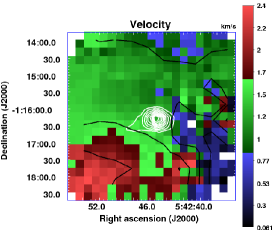
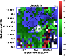
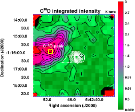
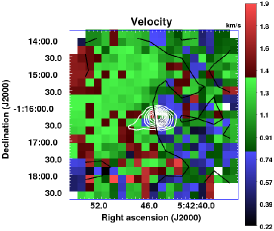
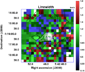
Figure 4: Same as Fig. 3 but for the 1.3-km s^-1 component. The black contours in the upper panels, from left to right, are plotted as follows: from 0.7 ($2.7\sigma$) to 7.0 K km s^-1 ($27\sigma$) in steps of 0.7 K km s^-1; at 0.5, 1, 1.5, and 2 km s^-1; and from 0.5 to 2.5 km s^-1 in steps of 0.5 km s^-1. In the lower panels, these contours are from 0.3 ($1.1\sigma$) to 2.7 K km s^-1 ($9.6\sigma$) in steps of 0.3 K km s^-1; at 0.5, 1, 1.5, and 2 km s^-1; and at 0.5, 1, and 1.5 km s^-1. The C¹⁸O peak position, from which the 1.3-km s^-1 component spectra were extracted (Sect. 3.4), is indicated by a yellow box in the left panels. The effective beam size $30\arcsec$ is shown in the lower left corner of the upper left panel.

3.3 Channel maps and PV plots

Velocity channel maps of the ¹³CO and C¹⁸O emission for the main velocity component are plotted in Figs. 5 and 6, respectively. As shown in these maps, extended ¹³CO emission can be seen across the velocity range $7.86<{\rm v}_{\rm LSR}<10.15$ km s^-1, while that of C¹⁸O extends over a somewhat narrower range of velocities, $8.32<{\rm v}_{\rm LSR}<9.78$ km s^-1.

Figure 7 shows a position-velocity (PV) diagram for ¹³CO$(2-1)$ emission with the direction of the cut shown in Fig. 3. The slice is taken through the entire mapped area, extending from the northwest corner to southeast corner, and its position angle, measured east of north, is P.A.$=135\degr$. As shown in the top middle panel of Fig. 3, the PV slice goes across the border of the velocity gradient. The presence of two velocity components at $\sim 8.5$ and $\sim 9.5$ km s^-1 are clearly visible in the PV plot. These velocities correspond to the NW and SE parts of the mapped area, respectively [the PV diagram of C¹⁸O emission (not shown) is essentially similar].

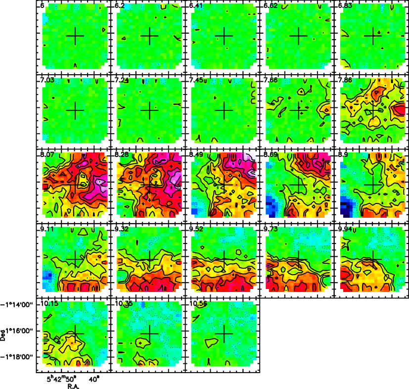
Figure 5: Velocity channel map across 6–10.56 km s^-1 of the ¹³CO$(2-1)$ line towards SMM 3. The velocity of each channel is shown in the top-left corner of each panel. The solid contours go from 0.67 to 4.67 K in steps of 0.67 K ($T_{\rm MB}$), while the dashed contours mirror negative values due to the baseline-fitting problems. The central cross on each panel indicates the map centre.

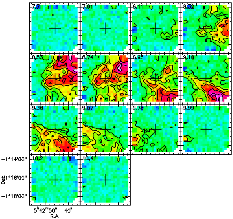
Figure 6: Same as Fig. 5 but across 7.7–10.41 km s^-1 of the C¹⁸O$(2-1)$ line. The contours are as in Fig. 5.

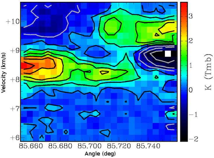
Figure 7: Position-velocity (PV) diagram of the ¹³CO$(2-1)$ emission towards the environment of SMM 3. The PV slice runs from NW to SE, across SMM 3, as shown in Fig. 3. The black contours go from 10 to 90% of the maximum value of 3.6 K, in steps of 10%. The grey contours represent negative values.

3.4 Spectra, line parameters, and column densities at the selected positions

We extracted individual ¹³CO and C¹⁸O spectra from the map centre, i.e., near the LABOCA 870-$\mu$m peak of SMM 3. Moreover, to investigate the properties of the lower-velocity component, we extracted the ¹³CO and C¹⁸O spectra from a peak position of C¹⁸O integrated intensity lying east of SMM 3 in projection (see the left panels of Fig. 4). The extracted spectra are shown in Fig. 8. The C¹⁸O line towards SMM 3 shows two nearby velocity components. There is a hint of that also in the ¹³CO spectrum. Moreover, the ¹³CO line appears to be blueshifted with respect to the C¹⁸O line, suggesting that the lines originate in two different gas layers along the line of sight. In the case of the lower velocity-component spectra (lower panel of Fig. 8), the ¹³CO line shows two velocity components around the systemic velocity of 1.38 km s^-1 derived from C¹⁸O$(2-1)$.

The line parameters of the extracted spectra are listed in Table 2. In this table, we give the offset of the target position from the map centre (in arcsec), radial LSR velocity (${\rm v}_{\rm LSR}$), FWHM linewidth ($\Delta{\rm v}$), peak intensity ($T_{\rm MB}$), integrated intensity ($\int T_{\rm MB}{\rm dv}$), peak line optical-thickness ($\tau_{0}$), and excitation temperature ($T_{\rm ex}$). The values of ${\rm v}_{\rm LSR}$ and $\Delta{\rm v}$ of the ¹³CO$(2-1)$ lines were derived through fitting the hyperfine structure of the line (see Cazzoli et al. (2004)), while those of C¹⁸O$(2-1)$ were obtained by fitting the lines with a single Gaussian. The two nearby velocity components were fitted simultaneously but for SMM 3 we only give the parameters of the components overlaid with green lines in Fig. 8. In contrast, in the case of the C¹⁸O peak of the lower velocity-component, we list the ¹³CO parameters of the component slightly redshifted from the C¹⁸O line velocity. The integrated line intensities listed in Col. (7) of Table 2 were computed over the velocity range given in square brackets in the corresponding column. This way, we were able to take the non-Gaussian features of some of the lines into account. The quoted uncertainties in ${\rm v}_{\rm LSR}$ and $\Delta{\rm v}$ are formal $1\sigma$ fitting errors, while those in $T_{\rm MB}$ and $\int T_{\rm MB}{\rm dv}$ were estimated by summing in quadrature the fitting error and the 10% calibration uncertainty.

The values of $\tau_{0}$ and $T_{\rm ex}$ for the lines towards the C¹⁸O peak of the lower velocity-component were derived as follows. By making the assumption that the ¹³CO and C¹⁸O emission arise from the same gas and the two transitions have the same beam filling factor and excitation temperature, we can numerically estimate the line optical thicknesses from the ratio of the line peak intensities as (e.g., Myers et al. (1983); Ladd et al. (1998))

$$\frac{T_{\rm MB}({\rm{}^{13}CO})}{T_{\rm MB}({\rm C^{18}O})}\approx\frac{1-e^{-\tau_{13}}}{1-e^{-\tau_{18}}}\,.$$ (1)

The peak intensities are used here rather than the integrated intensities because multiple velocity components could “contaminate” the latter values. To calculate the transition optical thicknesses, we used the CO isotopologue abundance ratio of

$$\frac{[{\rm{}^{13}CO}]}{[{\rm C^{18}O}]}=\frac{[{\rm{}^{13}C}]}{[{\rm{}^{12}C}]}\frac{[{\rm{}^{16}O}]}{[{\rm{}^{18}O}]}=\frac{1}{60}\times 500\simeq 8.3\,.$$ (2)

The adopted carbon- and oxygen-isotopic ratios are the same as those used in Paper III for a proper comparison to that work (see references therein). Consequently, the optical thickness ratio $\tau_{13}/\tau_{18}$ was assumed to be equal to 8.3.

Once the optical thickness is determined, $T_{\rm ex}$ can be calculated using the radiative transfer equation [see, e.g., Eq. (1) in Paper I]. In this calculation, we assumed a beam filling factor of unity, and that the background temperature is equal to the cosmic background radiation temperature of 2.725 K.

The derived values of $\tau_{13}$, $\tau_{18}$, and $T_{\rm ex}$ are listed on Cols. (8) and (9) of Table 2. In this table, we use the symbol $\tau_{0}$ for the optical thickness to denote its peak value. The quoted uncertainties were derived from the uncertainties of the peak intensities. The ¹³CO line appears to be optically thick, while the C¹⁸O line shows a moderate optical thickness of $\tau_{18}\simeq 0.8_{-0.2}^{+0.3}$.

The total beam-averaged ¹³CO and C¹⁸O column densities were computed following Eq. (4) of Paper I. The spectroscopic parameters needed in the analysis, such as the electric dipole moments and rotational constants, were adopted from the JPL database. The derived column densities are listed in the last column of Table 2. The quoted uncertainties were propagated from those associated with $T_{\rm ex}$, $\Delta{\rm v}$, and $\tau_{0}$ (the average value of the ${}^{+}_{-}-$errors of $T_{\rm ex}$ and $\tau_{0}$ were used).

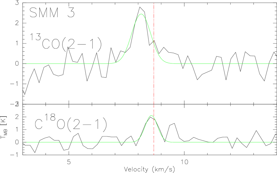
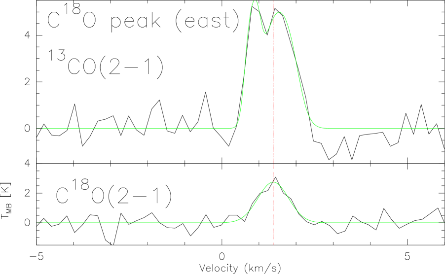
Figure 8: The ¹³CO$(2-1)$ and C¹⁸O$(2-1)$ spectra extracted towards SMM 3 (upper panel) and the position indicated in Fig. 4 (lower panel). Hyperfine-structure fits to the ¹³CO lines, and single Gaussian fits to the C¹⁸O lines are overlaid in green. The red dashed line overlaid on the spectra towards SMM 3 indicates the systemic velocity of SMM 3 as derived from C¹⁷O$(2-1)$ in Paper III. In the lower panel, the red dashed line shows the radial velocity of the C¹⁸O$(2-1)$ line.

Table 2: Parameters of the spectra extracted from the selected positions.

Position	Offset	Transition	${\rm v}_{\rm LSR}$	$\Delta{\rm v}$	$T_{\rm MB}$	$\int T_{\rm MB}{\rm dv}$	$\tau_{0}$	$T_{\rm ex}$	$N$
	$(\arcsec,\,\arcsec)$		[km s-1]	[km s-1]	[K]	[K km s-1]		[K]	[$10^{15}$ cm-2]
Main velocity component
SMM 3	$(0\,,0)$	13CO$(2-1)$	$8.11\pm 0.09$	$0.95\pm 0.36$	$2.73\pm 0.45$	$2.61\pm 0.67$ [7.17, 9.21]	-	-	-
		C18O$(2-1)$	$8.57\pm 0.05$	$0.63\pm 0.11$	$2.12\pm 0.25$	$1.39\pm 0.25$ [8.00, 9.14]	$0.2\pm 0.1$	$11.0\pm 1.0$	$0.85\pm 0.2$
Lower-velocity component
C18O peak	$(+85.5\,,+14.0)$	13CO$(2-1)$	$1.52\pm 0.06$	$0.81\pm 0.12$	$5.17\pm 0.61$	$7.05\pm 0.86$ [0.21, 2.38]	$6.3^{+2.4}_{-1.9}$	-	$18.2\pm 6.8$
		C18O$(2-1)$	$1.38\pm 0.06$	$0.97\pm 0.15$	$2.75\pm 0.61$	$2.89\pm 0.47$ [0.07, 2.52]	$0.8^{+0.3}_{-0.2}$	$9.5\pm 1.8$	$2.8\pm 1.0$

3.5 CO depletion in SMM 3

In Paper III, we derived a CO depletion factor of $f_{\rm D}=10.8\pm 2.2$ towards SMM 3 through C¹⁷O$(2-1)$ observations ($27\aas@@fstack{\prime\prime}8$ resolution). Another estimate of $f_{\rm D}$ in SMM 3 can be obtained from the current C¹⁸O data. We prefer to use C¹⁸O for this analysis rather than ¹³CO, because C¹⁸O emission is more optically thin than the ¹³CO emission. Therefore, C¹⁸O is expected to trace gas deeper into the core’s envelope, and being less affected by foreground emission.

The values of $\tau_{0}$ and $T_{\rm ex}$ for the C¹⁷O$(2-1)$ line were derived to be $0.05\pm 0.03$ and $11.0\pm 1.0$ K, respectively (Paper III). As the oxygen-isotopic ratio $[^{18}{\rm O}]/[^{17}{\rm O}]$ is only 3.52 (Frerking et al. (1982)), it can be assumed that the C¹⁸O$(2-1)$ line is also optically thin. Under the assumption of optically thin emission ($\tau\ll 1$), and adopting $T_{\rm ex}=11\pm 1$ K, the C¹⁸O column density computed from the integrated intensity is $N({\rm C^{18}O})=8.5\pm 1.7\times 10^{14}$ cm^-2.

By smoothing the LABOCA map to match the resolution of the C¹⁸O map ($30\arcsec$), and regridding it onto the same pixel scale, the 870-$\mu$m peak flux density towards the $(0\arcsec,\,0\arcsec)$ position of the C¹⁸O map is determined to be 0.85 Jy beam^-1. Using the assumption that $T_{\rm dust}=T_{\rm kin}$, and that the dust opacity per unit dust mass at 870 $\mu$m is $\kappa_{870}=1.7$ cm² g^-1 (Ossenkopf & Henning (1994); Paper I), we estimate that the corresponding H₂ column density is $N({\rm H_{2}})=2.5\pm 0.3\times 10^{22}$ cm^-2 (see Papers I and III for further details). Therefore, the fractional abundance of C¹⁸O towards the $(0\arcsec,\,0\arcsec)$ position is estimated to be $x({\rm C^{18}O})=N({\rm C^{18}O})/N({\rm H_{2}})=3.4\pm 0.8\times 10^{-8}$.

To compute $f_{\rm D}$ from C¹⁸O data, we need an estimate of the “canonical”, or undepleted, abundance of C¹⁸O. Using the standard value $9.5\times 10^{-5}$ for the abundance of the main CO isotopologue in the solar neighbourhood (Frerking et al. (1982)), we can write

$$x({\rm C^{18}O})_{\rm can}=x({\rm CO})_{\rm can}\times\frac{[{\rm{}^{18}O}]}{[{\rm{}^{16}O}]}=9.5\times 10^{-5}\times\frac{1}{500}=1.9\times 10^{-7}\,.$$ (3)

The value of $f_{\rm D}$ is then determined to be $f_{\rm D}=x({\rm C^{18}O})_{\rm can}/x({\rm C^{18}O})_{\rm obs}=5.6\pm 1.3$. This is comparable within a factor of two to the value derived from C¹⁷O$(2-1)$ data. The agreement is quite good given all the assumptions used in the analysis. We note that the $(0\arcsec,\,0\arcsec)$ position of the C¹⁸O map is not exactly coincident with our previous C¹⁷O observation target position but the two are within the beam size of both the observations.

Following the analysis presented in Miettinen (2012; Sect. 5.5 therein), the CO depletion timescale in SMM 3 is estimated to be only $\tau_{\rm dep}\sim 1-3.7\times 10^{4}$ yr [using the values $T_{\rm kin}=11.3$ K and $n({\rm H_{2}})=1.1-4.0\times 10^{5}$ cm^-3; see Table 1]. This provides a lower limit to the age of the core.

4 Discussion

4.1 On the non-detection of molecular outflows

Because SMM 3 is an early Class 0 source, it is expected to drive a bipolar molecular outflow. The outflows can manifest themselves in broad non-Gaussian spectral-line wings. One of our original attempts of the present study was to search for outflows driven by SMM 3 through ¹³CO observations. However, in our data, there is no evidence for a large-scale ¹³CO outflow. In the Spitzer/IRAC 4.5-$\mu$m image of SMM 3 (Fig. 1; bottom panel), there are some 4.5-$\mu$m emission features that could be signatures of shock-excited material around SMM 3 (e.g., Smith & Rosen (2005); De Buizer & Vacca (2010)). For comparison, the Class 0/I protostar IRAS 05399-0121 in Orion B9, which drives the HH 92 jet (Bally et al. (2002)), exhibits spectacular IRAC 4.5-$\mu$m features along its parsec-scale bipolar jet. Clearly, higher resolution observations, and better outflow tracers, such as ¹²CO and SiO, would be needed to clarify the outflow activity of SMM 3.

4.2 Low-velocity gas emission

As was discussed in Paper II (Sect. 5.7 therein), the lower-velocity line emission seen towards Orion B9 is likely to come from the “low-velocity part” of Orion B, which probably originates from the feedback from the massive stars of the nearby Ori OB 1b association. This fraction of the gas is likely to be located a few tens of parsecs closer to the Sun than the “regular” 9-km s^-1 gas component (Wilson et al. (2005)).

The C¹⁸O column density towards the selected C¹⁸O peak is $2.8\pm 1.0\times 10^{15}$ cm^-2. We can convert this to an estimate of the H₂ column density as

$$N({\rm H_{2}})=\frac{[{\rm H_{2}}]}{[{\rm{}^{12}CO}]}\times\frac{[{\rm{}^{12}CO}]}{[{\rm C^{18}O}]}\times N({\rm C^{18}O})\,.$$ (4)

Using again the values $[{\rm{}^{12}CO}]/[{\rm C^{18}O}]=[{\rm{}^{16}O}]/[{\rm{}^{18}O}]=500$ and $[{\rm{}^{12}CO}]/[{\rm H_{2}}]=9.5\times 10^{-5}$, we obtain $N({\rm H_{2}})=1.5\pm 0.5\times 10^{22}$ cm^-2. This shows that the “low-velocity part” of Orion B also consists of dense gas, which conforms to our previous detection of, e.g., deuterated molecular species at comparable LSR velocities. We also note that the prestellar core SMM 7 and Class 0 protostar IRAS 05413-0104 seen towards Orion B9 have such low systemic velocities ($\sim 3.7$ and $\sim 1.5$ km s^-1, respectively) that they are likely to be members of the low-velocity Orion B. Despite the estimated high column density of the clump-like ¹³CO/C¹⁸O feature seen in the left panels of Fig. 4, it was not seen in LABOCA 870-$\mu$m emission at the $\sim 3\sigma$ level (reflecting the strong CO depletion in the main velocity component).

4.3 On the origin of the velocity gradient and implications for the core/star formation in Orion B9

In Paper II, we speculated that the Orion B9 region has probably been influenced by the feedback from the nearby Orion OB association, or more precisely, from the Ori OB 1b subgroup. As mentioned above, this feedback is believed to be responsible for the “low-velocity part” of Orion B (Wilson et al. (2005)). We believe that the discovery of a velocity gradient in the present study supports the possibility that Orion B9 region is affected by stellar feedback.

To better illustrate the larger-scale view of the surroundings of Orion B9, in Fig. 9 we show a wide-field Herschel/SPIRE 250-$\mu$m image. A visual inspection of the image suggests that the Orion B9 region might be situated in quite a dynamic environment. Towards the south, there is the active massive star-forming region NGC 2024 some $40\arcmin$ ($\sim 5.2$ pc at 450 pc) from Orion B9. The northwest-southeast oriented 250-$\mu$m filament emanating from NGC 2024 is likely related to the dense molecular ridge of NGC 2024 running in the same direction (e.g., Thronson et al. (1984); Visser et al. (1998); Watanabe & Mitchell (2008)). The expanding H ii region of NGC 2024 appears to be interacting with the molecular ridge (Gaume et al. (1992)). The majority of the members of Ori OB 1b association lie towards the west/northwest from Orion B9 (see, e.g., Fig. 1 in Wilson et al. (2005)).

It is apparent from the bottom panel of Fig. 9 that the Orion B9 cores, with the possible exception of SMM 7, belong to a common northeast-southwest oriented filamentary structure. As indicated in the figure, the cores at the northeastern part of the region have a lower LSR velocity or show multiple velocity components as found in our previous papers. As discussed earlier, a gradient of increasing radial velocity from NW to SE is seen across the mapped area, and SMM 3 appears to lie on the border of the velocity jump [cf. the case of the Class 0 protostar HH211 in Perseus/IC348 (Tobin et al. (2011))]. Interestingly, this velocity gradient appears to be orthogonal to the direction of the 250-$\mu$m filament oriented NE-SW (SMM 3 also lies on the border of the dust filament). This raises the question whether this border could be tracing a shock layer of the interacting/colliding flows, within which there is a jump in the velocity of the gas. Such interaction might have been responsible for triggering the formation of SMM 3, and (some) of the other cores in the region. It seems more likely that, instead of the influence of Ori OB 1b, the feedback from the nearby expanding NGC 2024 H ii region could have compressed the inital cloud region (Fukuda & Hanawa (2000)). Later, the cloud under a high pressure gradient may have fragmented into dense cores, out of which some, such as SMM 3, were collapsed into protostars sequentially.

SMM 3 showed the highest level of CO depletion among the cores studied in Paper III. This conforms to the fact that it also appears to be the densest core in Orion B9. For the core collapse induced by compression, the simulations by Hennebelle et al. (2003) suggest that the combined duration of the prestellar$+$Class 0 phase is $\sim 3.2\times 10^{5}-1.3\times 10^{6}$ yr (depending on the rate of compression). As mentioned earlier, the estimated CO depletion timescale in SMM 3 is $\sim 1-3.7\times 10^{4}$ yr, which is shorter than the core evolution timescales quoted above. On the other hand, the fragmentation timescale of the core is expected to be comparable to the signal crossing time, which for SMM 3 is estimated to be $\tau_{\rm cross}=D/\sigma_{\rm 3D}\sim 6.6\times 10^{5}$ yr (the projected core diameter across the $3.3\sigma$ contour is $86\arcsec$ or $D=0.19$ pc, and $\sigma_{\rm 3D}=\sqrt{3}\sigma_{\rm 1D}$ is the three-dimensional velocity dispersion). This agrees well with the above theoretical core lifetimes. From these considerations, we suggest that the formation of SMM 3, and of some other cores in Orion B9, was triggered by feedback from NGC 2024 (dynamical compression) some several times $\sim 10^{5}$ yr ago (cf. Fukuda & Hanawa (2000)).

To better understand the velocity structure of the region on larger scales, larger maps of molecular-line emission would be needed. We note that the star formation in Orion B9, if triggered by stellar feedback, might resemble the situations in the $\rho$ Ophiuchus (e.g., Nutter et al. (2006)) and the B59/Pipe Nebula (Peretto et al. (2012)), where the star formation appears to be induced by the feedback from the Scorpius OB association.

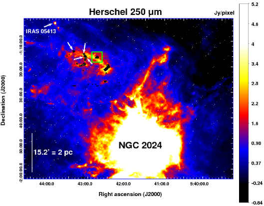
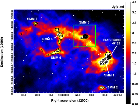
Figure 9: Top: A wide-field Herschel/SPIRE 250-$\mu$m far-infrared image towards the Orion B9 and NGC 2024 (Flame Nebula) star-forming regions. The image is overlaid with black contours of LABOCA 870-$\mu$m dust continuum emission. The contours go from 0.1 ($\sim 3.3\sigma$) to 1.0 Jy beam^-1 in steps of 0.1 Jy beam^-1. The green rectangle outlines the $4\arcmin\times 4\arcmin$ area mapped in ¹³CO$(2-1)$ and C¹⁸O$(2-1)$ in the present study. The white arrows indicate the cores which have a lower LSR velocity than the “main 9-km s^-1 part” of Orion B9 or show multiple velocity components. The Class 0 protostar IRAS 05413-0104 in the northeast corner was at the border of our LABOCA map and only weakly detected (see Fig. 1 in Paper I). Note how the Orion B9 cores are associated with a NE-SW oriented filamentary structure, and the cores with lower radial velocity (or with multiple velocity components) lie at the NE part of the structure. A scale bar indicating the 2 pc projected length is shown in the bottom left, with the assumption of a 450 pc line-of-sight distance. Bottom: A zoomed-in view of the upper image towards Orion B9. Selected cores are labelled. The LABOCA contours are as in the upper panel.

5 Summary and conclusions

A $4\arcmin\times 4\arcmin$ region around the Class 0 protostar SMM 3 in Orion B9 was mapped in ¹³CO and C¹⁸O $J=2-1$ lines with the APEX 12-m telescope. Our main results and conclusions can be summarised as follows:

1. Both lines exhibit two well separated velocity components: one at $\sim 1.3$ km s^-1 and the other at $\sim 8.7$ km s^-1. The latter is near the systemic velocity of SMM 3. The low-velocity component was already recognised in our previous studies, and it is believed to be related to the low-velocity part of Orion B.

2. The ¹³CO and C¹⁸O emission are relatively widely distributed compared to the dust continuum emission traced by LABOCA. The LABOCA 870-$\mu$m peak position of SMM 3 is not coincident with any strong ¹³CO or C¹⁸O emission, which is in accordance with the high CO depletion factor derived earlier by us from C¹⁷O$(2-1)$ ($f_{\rm D}\simeq 10.8$). The CO depletion factor derived from C¹⁸O data is within a factor of two from the previous estimate, i.e., $f_{\rm D}\simeq 5.6$. No evidence for a large-scale outflow activity, i.e., high velocity line wings, was found towards SMM 3.

3. The lower-velocity ($\sim 1.3$ km s^-1) ¹³CO and C¹⁸O emission are concentrated into a clump-like feature at the eastern part of the map. We estimate that the H₂ column density towards its C¹⁸O maximum is $\sim 10^{22}$ cm^-2. Therefore, the lower-velocity gas seen along the line of sight is of high density, which is consistent with our earlier detection of, e.g., deuterated molecular species (DCO⁺, N₂D⁺).

4. We observe a velocity gradient across the ¹³CO and C¹⁸O maps along the NW-SE direction (some hint of that is also visible in the lower-velocity line maps). Interestingly, SMM 3 is projected almost exactly on the border of the velocity jump. The sharp velocity-gradient border provides a strong indication that it represents an interaction zone of flow motions.

5. We suggest a possible scenario in which the formation of SMM 3, and likely some of the other dense cores in Orion B9, was triggered by an expanding H ii region of NGC 2024. This collect-and-collapse -type process might have been taken place some several times $10^{5}$ yr ago. The NGC 2024 region is known to be a potential site of induced, sequential star formation (e.g., Fukuda & Hanawa (2000), and references therein). The case of Orion B9 suggests that we may be witnessing the most recent event of self-propagating star formation around NGC 2024. Larger-scale molecular-line maps would be needed for a better understanding of the larger-scale velocity structure of the region.