Economics of Electric Vehicle Charging: A Game Theoretic Approach

Abstract

In this paper, the problem of grid-to-vehicle energy exchange between a smart grid and plug-in electric vehicle groups (PEVGs) is studied using a noncooperative Stackelberg game. In this game, on the one hand, the smart grid that acts as a leader, needs to decide on its price so as to optimize its revenue while ensuring the PEVGs’ participation. On the other hand, the PEVGs, which act as followers, need to decide on their charging strategies so as to optimize a tradeoff between the benefit from battery charging and the associated cost. Using variational inequalities, it is shown that the proposed game possesses a socially optimal Stackelberg equilibrium in which the grid optimizes its price while the PEVGs choose their equilibrium strategies. A distributed algorithm that enables the PEVGs and the smart grid to reach this equilibrium is proposed and assessed by extensive simulations. Further, the model is extended to a time-varying case that can incorporate and handle slowly varying environments.

I Introduction

Due to the growing concerns for energy conservation and the environment, it is expected that plug-in electric vehicles (PEVs) will play a major role in the future smart grid (SG) [2]. Therefore, several countries are working on establishing novel PEV policies and plans because of their significant environmental advantages and cost savings [3].

The deployment of PEVs will introduce new challenges in the design of SGs. These challenges include developing optimal charging strategies for the connected PEVs, ensuring efficient communications between PEVs and the grid, and managing energy exchange between regular loads of the grid and the PEVs. In [2], the optimal charge control of PEVs is analyzed in deregulated electricity markets based on a forecast of future electricity prices and the optimal economic solution for the vehicle owner. In [4], a real-time pricing algorithm is proposed for smart grids considering smart meter and energy provider interaction through control messages exchange. A noncooperative game model for pricing and frequency regulation in smart grids with electric vehicles is studied in [5]. Using facility location games, in [6], optimal locations of battery exchange stations were derived within a vehicle-to-grid (V2G) network. An optimization framework is proposed in [7] for enabling the SG to determine the time and duration of the PEVs charging. In [8], a control algorithm is developed based on queuing theory to control the charging of PEVs. A stochastic programming technique is introduced in [9] to show the impact of charging PHEVs on a residential distribution grid. The issue of vehicle-to-grid (V2G) integration and the prospective communication interface to enable this integration are addressed in [10]. In [11], a mean field game is proposed to investigate the competitive interaction between electric vehicles in a Cournot market consisting of electricity transactions to/ from an electricity distribution network. To manage a large number of PHEVs at a municipal parking station, an algorithm using particle swarm optimization is proposed in [12]. An intelligent method for scheduling the usage of the available storage capacity from PHEVs and electric vehicles is proposed in [13]. Other aspects of electric vehicles in smart grids in terms of energy storage, charging and greenhouse gas emission reduction are discussed in [14, 15, 16]. Beyond PEVs, many possible demand side management solutions are also foreseen for the smart grid [17] and each of these solutions has a number of benefits and cost tradeoffs. Subsequently, it is anticipated that many of these solutions, including the incorporation of electric vehicles, will co-exist to provide smart energy management for the power grid.

One of the key challenges of widespread penetration of PEVs in the power network is the choice of an optimal charging strategy for the PEVs. This is mainly due to the fact that the integration of the PEVs into the network has a major impact on the power grid and can potentially double the average load [4, 18]. The simultaneous charging of several PEVs in a particular area can overload the network and, thus, lead to an interruption of services for other consumers. The problem of PEV charging and its impact on the power distribution grid and electricity market have been addressed in [2, 1, 3, 8, 7] and [19]. However, little has been done to develop distributed models and algorithms that can capture the interactions between PEVs and the grid, in a grid-to-vehicle scenario. There is a need to develop solutions that capture the often conflicting objectives between the SG, which seeks to maximize its revenue, and the PEVs, which seek to optimize their charging behavior. Because of the limited grid capacity and PEVs’ energy demands, it is of interest to develop a model that can capture the decision making process of the PEVs and the grid when the grid’s limited energy needs to be allocated among the PEVs based on their needs.

The main contribution of this paper is to provide a comprehensive analytical framework that is suitable for capturing the interactions between an SG and a number of PEV groups (PEVGs), e.g., parking lots, which must decide on their charging profiles. We model the problem as a generalized Stackelberg game in which the SG is the leader and the PEVGs are the followers. The objective of the PEVGs is to strategically choose the amount that they need to charge, so as to optimize a utility that captures the tradeoff between the charging benefits and the associated costs, given various practical constraints on the PEVGs and the main grid. Based on the strategy choices of the PEVGs, the leader aims to optimize its price so as to maximize its revenues. We analyze the properties of the resulting game within the studied model, including existence of an equilibrium and optimality, and show that there exists an efficient (i.e., socially optimal) generalized Stackelberg equilibrium. We show that, due to the coupled capacity constraints between the PEVGs, the noncooperative followers’ game leads to a generalized Nash equilibrium, and the solution enables the capture of not only the charging behavior of the vehicles but also the decisions made by the SG. We propose a novel algorithm that the PEVGs and the grid can use, in a distributed manner, so as to reach the desired equilibrium. We also show that the proposed algorithm enables the system to adapt to time-varying environmental conditions such as arrival/departure of PEVs. Using extensive simulations, we assess the properties of the proposed scheme.

The rest of this paper is organized as follows. Section II describes the system model. In Section III, we formulate the noncooperative generalized Stackelberg game and we discuss its properties. In Section LABEL:solutionGame, we propose a distributed algorithm for finding the equilibrium. Adaptation of the proposed game to time-varying conditions is discussed in Section LABEL:dynamic-case. Numerical results are analyzed in Section VI and conclusions are drawn in Section VII.

II system model

Consider a power system consisting of a single power grid (i.e., an SG), several primary and secondary load subscribers or consumers and a smart energy manager (SEM). Here, the SG refers to the main electric grid which is connected to the area of interest via one or more substations. Further, we consider that the SG is servicing a certain area or groups of primary consumers such as industries, houses and offices. After meeting the demands of the primary consumers the grid wishes to sell its excess of energy (if any) to the secondary users, such as PEVs, connected to it in that area. Consider a number of groups of PEVs (hereinafter, we use the term PEVG to denote a group of PEVs, acting as a single PEV entity), which are connected to the grid at peak hours of energy demand e.g., from $12$ pm to $4$ pm [20]. The total charging period for the PEVGs is considered to be divided into multiple time slots. Each time slot has a duration of anywhere between $5$ minutes and half an hour based on the changing traffic conditions of the PEVs in the group [21]. For a particular time slot, the power grid has a maximum energy $C$ that it can sell to the connected ${N}$ PEVGs, allowing them to meet their demand. The power grid will set an appropriate price $p$ (per unit of energy) for selling its surplus so as to optimize its revenue.

Each PEVG $n\in\mathcal{N}$, where $\mathcal{N}$ is the set of all $N$ PEVGs, will request a certain amount of energy $x_{n}$ from the grid so as to meet its energy requirements (e.g., to go back home after office work). This demand of energy may vary for the PEVs in the group based on different parameters such as the battery capacity $b_{n}$ of the PEVG, the available energy in the PEVG’s battery at the time of plug-in to the grid, the price $p$ per unit of electricity and the nature of usage (e.g., two identical PEVGs with different travel plans may need different amounts of energy). During peak hours, the available energy for servicing PEVGs is often limited [20], and, thus, the PEVGs will request only the amount needed due to their immediate need for charging. Since the net energy $C$ available for the PEVGs at the grid is fixed, the demands of the PEVGs must satisfy

$$\sum_{n}x_{n}\leq C.$$ (1)

Given the amount requested by the PEVGs, the SG sets a price $p$ per unit of energy so as to optimize its revenue from selling energy by strategically choosing its price per unit of energy. Although the SG can choose the price $p$ within any range to maximize its total revenue, a very large $p$ may compel a PEVG to withdraw its demand from the grid and to search for alternate markets or wait until the prices drop. Therefore, an optimal price needs to be chosen by the grid operator which is not very high (to avoid losing customers) and not very low (to avoid losing revenue), in an effort to maximize its profit.

To successfully complete the energy trading, the PEVGs and the grid interact with each other and agree on the energy exchange parameters, such as the selling price and the amount of energy demanded, that meet the objectives of the both sides. The amount of requested energy $x_{n}$ is determined by the physical characteristics of PEVG $n$ as well as by the tradeoff between the potential benefit that PEVG $n$ is expecting from buying $x_{n}$ and the selling price $p$ of the grid. Moreover, the selling price $p$ per unit of energy is strongly dependent upon the amount demanded by the PEVGs as well as the number of PEVGs that are connected to the grid. This is due to the fact that the amount of energy available from the grid is fixed and, thus, as the number of PEVGs increases, the amount that each PEVG can acquire becomes smaller. As a result, the grid can set a higher price to increase its revenues.

It is clear that the demands of the connected PEVGs are coupled through the energy constraint in (1), and are also dependent on the physical characteristics and capabilities of the PEVGs. Also it is important to note that the price set by the grid is dependent on the demand of each PEVG. Thus, the main challenges faced when developing an approach that can successfully capture the decision making process of both the PEVGs and the grid are: i)- modeling the decision making processes and the interactions between the connected PEVGs in the network given the constraint in (1); ii)- developing an algorithm that enables the PEVGs in the network to strategically decide on the amount of energy that they will request from the grid so as to optimize their satisfaction levels given the constraint in (1); and iii)- enabling the grid to optimize its price while capturing the tradeoff between the PEVGs’ participation and revenue maximization. To address these challenges we propose a framework based on noncooperative game theory.

III Noncooperative generalized Stackelberg game

III-A Game formulation

To formally study the interactions between the SG and the PEVGs, we use a Stackelberg game [22] which is a type of noncooperative game that deals with the multi-level decision making process of a number of independent decision makers or players (followers) in response to the decision taken by a leading player (the leader) [22]. Hence, we formulate a noncooperative Stackelberg game in which the SG is the leader and the PEVGs are the followers. This game is defined by its strategic form, $\Gamma=\left\{(\mathcal{N}\cup\{\text{SG}\}),\left\{X_{n}\right\}_{n\in\mathcal{N}},\left\{U_{n}\right\}_{n\in\mathcal{N}},L(p),p\right\}$, having the following components:

1. The PEVGs in $\mathcal{N}$ act as the followers in the game and respond to the price set by the SG.

2. The strategy of each PEVG $n\in\mathcal{N}$ which corresponds to the amount of energy demanded $x_{n}\in\mathbf{X_{n}}$ from the grid satisfying the constraint $\sum_{n}x_{n}\leq C$.

3. The utility function $U_{n}$ of each PEVG $n$ that captures the benefit of consuming the demanded energy $x_{n}$.

4. The utility function $L(p)$ for the SG (leader of the game), which captures the total profit that the grid can receive by selling the surplus energy with price $p$.

5. The price $p$ per unit of energy charged by the SG.

III-A1 Utility Function of a PEVG

For each PEVG $n\in\mathcal{N}$, we define a utility function $U_{n}(x_{n},\mathbf{x_{-n}},s_{n},b_{n},p)$, which represents the level of satisfaction that a PEVG obtains as a function of the energy it consumes. Here $b_{n}$ is the battery capacity of PEVG $n$ and $x_{n}$ is the requested energy from the grid; $s_{n}$ is the satisfaction parameter of PEVG $n$, which is a measure of the satisfaction the PEVG can achieve from consuming one unit of energy. This $s_{n}$ may depend on PEVG’s battery state at the time of plug-in to the grid, the available energy at the grid and/or the travel plan of the corresponding PEVG. For example, a PEVG $1$ having less need for energy than another PEVG $2$ (e.g., due to having a fuller battery) will need less energy than PEVG $2$ to attain the same satisfaction level (i.e., $s_{2}<s_{1}$). The energy demand may vary based on the battery capacity and/or the satisfaction parameter of each PEVG. The price per unit of energy can also affect the demand of the PEVG. Thus, the properties that the utility of a PEVG must satisfy are as follows:

1. The utility functions of the PEVGs are considered to be non-decreasing because each PEVG is interested in consuming more energy if possible unless it reaches its maximum consumption level. Mathematically,

   $$\frac{\delta U_{n}(x_{n},\mathbf{x_{-n}},s_{n},b_{n},p)}{\delta x_{n}}\geq 0.$$ (2)

2. The marginal benefit of a PEVG is considered as a non-increasing function, as the level of satisfaction of the PEVGs gradually gets saturated as more energy is consumed, i.e.,

   $$\frac{\delta^{2}U_{n}(x_{n},\mathbf{x_{-n}},s_{n},b_{n},p)}{\delta{x_{n}}^{2}}\leq 0.$$ (3)

3. Hereinafter, we consider that, for a fixed consumption level $x_{n}$, a larger $b_{n}$ implies a larger $U_{n}(x_{n},\mathbf{x_{-n}},s_{n},b_{n},p)$ and a larger $s_{n}$ leads to a smaller $U_{n}(x_{n},\mathbf{x_{-n}},s_{n},b_{n},p)$. So we have

   $$\frac{\delta U_{n}(x_{n},\mathbf{x_{-n}},s_{n},b_{n},p)}{\delta b_{n}}>0,$$ (4)

   and

   $$\frac{\delta U_{n}(x_{n},\mathbf{x_{-n}},s_{n},b_{n},p)}{\delta s_{n}}<0.$$ (5)

4. The price per unit of energy set by the grid affects the utilities of the PEVGs and the utility of a PEVG decreases with a higher price. That is,

   $$\frac{\delta U_{n}(x_{n},\mathbf{x_{-n}},s_{n},b_{n},p)}{\delta p}<0.$$ (6)

In this work we consider the particular utility

$$U_{n}(x_{n},\mathbf{x}_{-n},s_{n},b_{n},p)=b_{n}x_{n}-\frac{1}{2}s_{n}{x_{n}}^{2}-px_{n},$$ (7)

where $x_{n}\in[0,C-\sum_{k=1,k\neq n}^{N}x_{k}]$ and $\mathbf{x_{-n}}=[x_{1},x_{2},...,x_{n-1},x_{n+1},...,x_{N}]$, although many of our results can be generalized.

From (7), the utility of PEVG $n$ is affected by its battery capacity $b_{n}$. This is due to the fact that a PEVG with higher $b_{n}$ will have higher marginal utility and thus, needs to consume more energy to reach its maximum satisfaction level [23]. The utility also depends on the satisfaction parameter $s_{n}$ of the PEVG. PEVGs with the same capacity but with a different satisfaction parameter will have different marginal utilities and, thus, will be satisfied by different amounts of energy. To this end, we assume that a PEVG does not consume any energy beyond its maximum satisfaction level, i.e., $U_{n}=0$ if $x_{n}>({x_{n}}^{*}-x_{n}^{\text{ini}})$, where $x_{n}^{\text{ini}}$ is the initial energy in PEVG’s battery at the time of plug-in to the grid and ${x_{n}}^{*}$ is the energy that maximizes its utility within the given constraint in (1).

III-A2 Utility Function of the Power grid

A PEVG $n$ that consumes $x_{n}$ MWh of electricity during a designated period of time at a rate $p$ per MWh is charged $px_{n}$ which is the cost imposed by the SG on the PEVG. The objective of the SG is to maximize its revenue by selling the available energy surplus to the PEVGs after meeting the demand of its primary consumers, and also to control the nature of energy consumption of the PEVGs. While this energy surplus $C$ is fixed, the SG wants to set a price $p$ per unit of energy so as to optimize its revenue, given the demands of the PEVGs. Thus, we assume the utility function for the grid is

$$L(p,x_{n}(p))=p\sum_{n}x_{n},$$ (8)

which captures the total revenue of the grid when selling the energy required by all PEVGs at a price $p$ per unit of energy.

In this proposed game, the SG can control the price $p$ per unit of energy it wishes to sell. Connected PEVGs respond to the price by demanding a certain amount of energy, given the constraint in (1), so as to maximize their utilities. Thus, for a fixed price $p$, the objective of any PEVG $n$ is

$$\displaystyle\max_{x_{n}\in(C-\mathbf{x_{-n}})}U_{n}(x_{n},\mathbf{x_{-n}},s_{n},b_{n},p),$$

$$\text{s. t.}~{}\displaystyle\sum_{n}x_{n}\leq C.$$ (9)

Here, we can see that the amount of energy demanded by each PEVG $n$ depends, not only on its own strategies and price but also on the demand of other PEVGs in the network through (1) and the constraint is the same for all players. This leads connected PEVGs to engage in a noncooperative resource sharing game, which is a jointly convex generalized Nash equilibrium problem (GNEP) due to the same shared constraint (1). Note that, in game theory, a noncooperative game in which the players’ actions are coupled solely through the constraints, such as in the proposed model, is a special class of games whose solution is the generalized Nash equilibrium [24, 25], and hence, the proposed followers’ game, for any price $p$, is a noncooperative resource sharing game whose solution is the generalized Nash equilibrium (GNE). Then, given all the PEVGs’ demands are at the GNE, the leader, i.e., the grid, chooses the price to maximize its revenue. Thus, for the given GNE demands of the PEVGs, the objective of the grid is

$$\displaystyle\max_{p}L(p)=\displaystyle\max_{p}\displaystyle\sum_{n}px_{n}.$$ (10)

Thus, one suitable solution for the formulated game $\Gamma$ is the Stackelberg equilibrium at which the leader reaches its optimal price, given the followers’ optimal response at their GNE. At this equilibrium, no player (leader or follower) can improve its utility by unilaterally changing its strategy. In classical Stackelberg games, the followers typically choose their Nash equilibrium strategies. In our model, due to the coupled strategies as per (1), the PEVGs need to seek a GNE instead of a classical Nash equilibrium. To this end, hereinafter, we refer to our game as a generalized Stackelberg game (GSG) whose solution is the generalized Stackelberg equilibrium (GSE) in which the followers reach a GNE.

Definition 1

Consider the GSG $\Gamma=\left\{(\mathcal{N}\cup\textrm{SG}),\left\{X_{n}\right\}_{n\in\mathcal{N}},\left\{U_{n}\right\}_{n\in\mathcal{N}},L(p),p\right\}$ defined in III-A where $U_{n}$ and $L(p)$ are given by (7) and (8) respectively. A set of strategies ($\mathbf{x^{*}},p^{*}$) constitutes the GSE of this game, if and only if it satisfies the following set of inequalities:

$$U_{n}({x_{n}}^{*},\mathbf{{x_{-n}}^{*}},s_{n},b_{n},p^{*})\geq U_{n}({x_{n}},\mathbf{{x_{-n}}^{*}},s_{n},b_{n},p^{*}),$$

$$\forall{x_{n}}^{*}\in\mathbf{x^{*}},\hskip 5.69046ptn\in\mathcal{N},\sum_{n}x_{n}\leq C$$ (11)

and

$$L(p^{*},\mathbf{x^{*}})\geq L(p,\mathbf{x^{*}}).$$ (12)

Thus, when all the PEVGs’ demands are at the GSE, no PEVG can improve its utility by deviating from its GSE demand and similarly, no price other than the optimal price $p^{*}$ set by the grid at the GSE, can improve the utility for the grid.

III-B Existence and efficiency of GSE

In noncooperative games, the existence of an equilibrium solution (in pure strategies) is not always guaranteed [22]. Therefore, for our follower game, we need to investigate the existence of the GNE in response to a price $p$. Specifically, we are interested in investigating the existence and properties of a variational equilibrium (VE), which is a type of GNE to be defined below (see also [24]), for our case. This is due to the fact that a VE is more socially stable than another GNE (if there exists any) and thus, is a desirable target for any algorithm to achieve [25]. Particularly for the proposed case, where a number of PEVGs in the SG network are demanding energy from a constrained reserve, an efficient VE would be the most appropriate solution to be considered. Hereinafter, we use VE and GNE interchangeably.

Consequently, the state transition equation for the time-varying system can be defined as [34]

$$C_{t+1}=f_{t}(C_{t},p_{t},\mathbf{x^{t}}),~{}t=0,1,2,...,T-1,$$ (34)

where $t$ is an integer time index, and $T$ is the entire peak hour duration. For a feedback Stackelberg game, $C_{t}$ is the information about the available energy supply at time $t$, which is gained by the grid from (34) and fed back to the PEVGs through the SEM [34]. The state of available energy supply at any instant $t$ is a function of the demand for energy by the PEVGs, and the energy available at the previous time slot. The state transition from $t$ to $t+1$ takes place when a change occurs either in the number of PEVs in the PEVG, or in the available energy from the grid. The objective of both the SG and the PEVGs is to choose their strategies so as to maximize their utilities in each time interval, and thus to maximize their total payoffs in the entire time horizon of peak hours. Hence, the problems of payoff maximization of the players for a discrete time feedback Stackelberg game can be formally expressed as

$$\max L_{T-t}=\sum_{t}\max_{p_{t}}p_{t}\sum_{n}x_{t}^{n},$$ (35)

for the SG, and

$$\max U_{T-t}=\sum_{t}\max_{x_{t}^{n}}\sum_{n}\left(b_{n}^{t}x_{n}^{t}-\frac{1}{2}s_{n}^{t}{x_{n}^{t}}^{2}-p_{t}x_{n}^{t}\right)$$ (36)

$$~{}\sum_{n}x_{n}^{t}\leq C_{t}~{}\text{at}~{}t=0,1,2,...,T,$$

for the PEVG $n$. The objective functions in (35) and (36) refer to a feedback Stackelberg game with Nash game constraints in the lower level decision making process [32] (similar to the game proposed in Section III for a single time instant) over the whole time horizon. Here, we assume that the leader of the game can perfectly gain the information about $C_{t}$ from (34) [35]. At any instant $t$, the SG gets the information about the volume of the parking lot (i.e., $b_{n}^{t-1}$ and $s_{n}^{t-1}$ for all $n=1,2,..,N$), the demand of the PEVGs in the previous time slot $t-1$ as well as the per unit price $p_{t-1}$. Then, it estimates the amount of energy that needs to be provided to the PEVGs at $t$ through (34). The SG feeds $C_{t}$ back to the PEVGs through the SEM and the PEVGs play the jointly convex generalized Nash game of Algorithm LABEL:algorithm1 for the allocation of energy within $\sum_{n}x_{n}^{t}\leq C_{t}$.

Here, $(\mathbf{x^{1}}^{*},\mathbf{x^{2}}^{*},...,\mathbf{x^{T}}^{*})$ and $(p_{1}^{*},p_{2}^{*},...,p_{T}^{*})$ constitute the solution of the discrete time Stackelberg game under a feedback information structure with the corresponding state information $(C_{1},C_{2},...,C_{T})$, if $\mathbf{x}{{}^{t}}^{*}$ comprises the solution of the GNE among the followers for price $p_{t}^{*}$ at each $t=1,2,...,T$ [32]. The solution will be team optimal if the solution at the GNE is optimal, that is if the GNE is a VE [24], for the sub game in each $t=1,2,...,T$ [32]. Now, given that the Stackelberg game described in Section III constitutes a sub-game in each time interval $t$ of the feedback Stackelberg game, the sub-game will reach its optimal solution (as shown in Section III-B) within the constraint $\sum_{n}x_{n}^{t}\leq C_{t}$ at each $t=1,2,...,T$. Therefore, the solution of the discrete time feedback Stackelberg game possesses a team optimal solution.

VI Numerical analysis

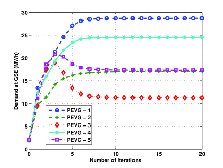
Figure 1: Convergence of the demand of each PEVG to the GSE.

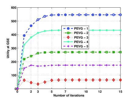
Figure 2: Convergence of the utility of each PEVG to the GSE.

For our simulations, we consider a number of PEVGs that are connected to the grid during peak hours. Here, a single PEVG entity represents $1000$ vehicles at a specific location [2], where each single vehicle is assumed to require $22$ kWh for every $100$ miles [36, 37]. The maximum battery capacity of any single vehicle is chosen between $150$ and $300$ miles. Hence, the maximum capacity $b_{n}$ of any PEVG $n$ ranges between $35$ MWh and $65$ MWh, which is chosen randomly for each PEVG. The available energy at the grid is chosen as $99$ MWh. Initially, the grid sets the selling price to $17$ USD per MWh. We note that the chosen parameters correspond to a typical PEVG use case [2, 36, 37]. However, we duly highlight that these parameters can vary considerably according to PEVG usage and type, and economic conditions within a given city, or country.

The satisfaction parameter $s_{n}$ is chosen randomly in the range of [$1,2$]. The range of $s_{n}$ is chosen based on the assumption that the PEVG with the lowest satisfaction parameter $s_{n}=1$ will get full satisfaction from each unit of energy it will consume whereas the PEVG with the highest parameter i.e., $s_{n}=2$, will reach the same satisfaction level from consuming half the amount due to its smaller limitations in terms of its initial battery state and travel plan. We do not consider the PEVGs with $s_{n}>2$ as they do not have an immediate need for energy at the peak hour. All statistical results are averaged over all possible random values of the PEVGs’ capacities using around $1000$ independent simulation runs.

In Fig. 1 and Fig. 2, we show the demand and the utility at the GSE for a network with ${N}=5$ PEVGs. Here, we can see that a similar demand by different PEVGs does not always lead to a similar utility for the PEVGs. For example, although PEVGs $2$ and $5$ in Fig. 1 have almost the same demand at the GSE, their utilities are different from one another as shown in Fig. 2. This is due to their different battery capacities and satisfaction parameters. From the utility in (7), we can see that the maximum utility level of a PEVG varies significantly for different values of $b_{n}$ and $s_{n}$. Therefore, with the same energy consumption, different PEVGs may obtain a different utility (e.g., PEVGs $2$ and $5$). Fig. 1 and 2 show that, after the $10^{\text{th}}$ iteration, all the PEVGs reach their maximum utilities, and, thus, their demands converge to the GSE.

In Fig. 3, we analyze the convergence speed of the proposed algorithm by plotting the values of $\lambda_{n}$ as a function of the number of iterations for $N=5$ PEVGs. First, recall that the demands of all PEVGs converge to GSE for the optimal price $p^{*}$ when all the PEVGs reach their VE and at this VE $\lambda_{n}=\lambda\geq 0,~{}\forall n$. Fig. 3 shows that our algorithm converges to the GSE after $9$ iterations (i.e., the PEVGs reach their VE). Hence, as shown by Fig. 3, the convergence speed of our algorithm is reasonable.

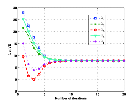
Figure 3: Convergence of the values of $\lambda_{n},~{}\forall n$ to $\lambda\geq 0$ as the solution of the GSG converges to GSE.

In Fig. 4, we show how the price set by the grid converges to its optimal value as the strategies of the PEVGs converge to the VE for networks of various sizes ($N=5,10$, and $15$ PEVGs) with an initial SG price set to $17$ USD per unit of energy. Fig. 4 shows that the price converges to an approximate optimal value within $5$ iterations. This is due to the fact that the SG sets its price in response to the demand strategies of the PEVGs. In fact, the PEVGs reach an approximate GSE within five iterations, as shown for $5$ PEVGs in Fig. 1, and, then, they optimize their demands within constraint (1). The PEVGs eventually reach the unique GSE that maximizes their utilities under this constraint. Hence, the price $p$ converges quickly to its optimal value $p^{*}$.

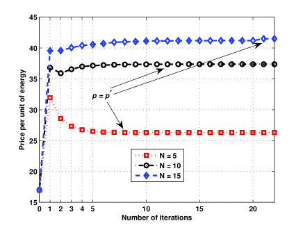
Figure 4: Convergence of the price per unit of energy to the optimal price for a network with different numbers of PEVGs.

Furthermore, Fig. 4 shows that the variation of the grid’s price is more noticeable when fewer PEVGs exist. This is due to the fact that, for a fixed grid capacity, as the number of PEVGs increases, there are fewer possibilities of variations in the demands due to (1).

In Fig. 5, we show the effect of the number of PEVGs on the optimal price choice of the grid. To do so, we increase the number of PEVGs in the network for different grid capacities $C=60,80$ and $90$ MWh. Fig. 5 shows that the average optimal price increases with the number of PEVGs in the network because of the increasing energy demand on the SG’s limited resources.

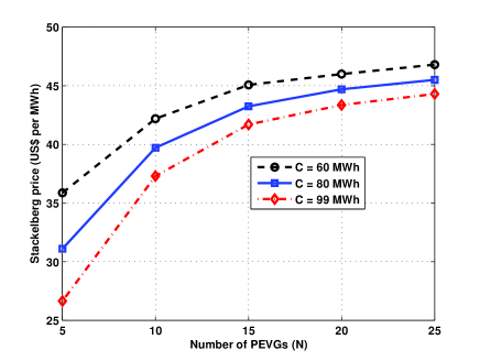
Figure 5: Effect of increasing the number of PEVGs ${N}$ in the network and the grid energy $C$ on the average Stackelberg price.

In contrast, increasing the grid’s capacity leads to a decrease in the optimal price $p^{*}$. This is due to the fact that, as the total available capacity of the grid increases, the grid has more energy to sell and, thus, it can decrease its price while maintaining desirable revenues. Moreover, for a fixed number of PEVGs, as the available energy at the grid increases, the SG reduces its optimal price to encourage the PEVGs to demand more energy.

Fig. 6 shows the average and maximum number of iterations needed to reach the GSE of the proposed game with respect to the number of PEVGs.

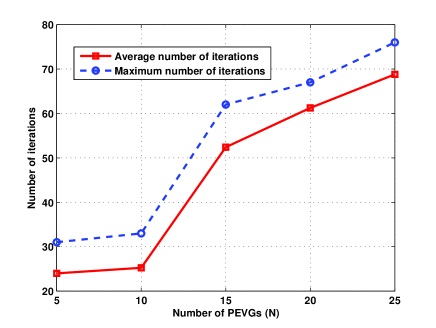
Figure 6: Effect of increasing the number of PEVGs on the average and maximum number of iterations to reach the GSE.

In Fig. 6, we can see that, whenever the number of PEVGs in the network increases, for the same amount of capacity from the grid, the PEVGs require more iterations to reach their optimal demands. For example, when the number of PEVGs in the network increases from $15$ to $25$, the average number of iterations needed to reach the GSE increases from $52$ to $79$. Similar behavior is also seen for the maximum number of iterations.

In Fig. 7, we compare the results of the proposed scheme with a particle swarm optimization (PSO) [12] and an equal distribution (ED) scheme [39]. In a PSO scheme, a group of random solutions (i.e., particles) are scattered over the search space, and the particles converge to a near optimal solution after a number of iterations. For the PSO algorithm, the particle size is considered to be $40$. The parameters are updated in such a way that the constraint in (1) is satisfied. For the ED scheme, the available grid energy is distributed equally among the connected PEVGs in the network. That is, if the available energy at the grid is $C$ MWh and there are $N$ PEVGs connected to the grid, then each PEVG receives an allocation of $\frac{C}{{N}}$ MWh of energy from the grid as long as this allocation does not exceed the maximum that a PEVG can be charged.

Fig. 7 shows that the average utility achieved by the proposed scheme is better for most of the PEVGs in the network, except PEVGs $9$ and $10$, when compared to the PSO scheme. This is due to the fact that the PSO scheme optimizes the energy for each PEVG according to the better particle position in the available energy space. This may lead to a better utility for PEVGs $9$ and $10$ at the expense of much lower utilities for the rest of the PEVGs. However, the proposed scheme allocates the energy among the PEVGs so that the socially optimal solution is achieved. Therefore, most of the PEVGs in the network achieve improved utilities compared with the PSO scheme. From Fig. 7, the proposed scheme has a total utility, on the average, $1.3$ times the utility achieved by the PSO scheme. Moreover, the proposed scheme has, on the average, twice the utility achieved by the ED scheme which is a significant improvement.

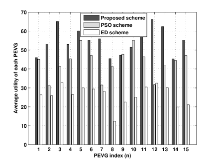
Figure 7: Comparison of the average utilities of the PEVGs at the GSE for the proposed scheme, the PSO scheme and ED scheme.

Fig. 8 shows the average demand per PEVG as the number of PEVGs varies. In Fig. 8, we can see that the average demand per PEVG decreases as the number of PEVGs increases. This is a direct result of (1) and of the fact that the optimal price set by the grid increases as the number of PEVGs increases. From Fig. 8, we can see that average PEVG demand for our scheme, the PSO scheme, and the ED case decreases as the number of PEVGs increases. Fig. 8 shows that the energy demand for the proposed scheme is lower than that for both the PSO and ED scheme for all $N$. This can be interpreted by the fact that, in our proposed scheme, each PEVG demands a required amount of energy within constraint (1) based on its satisfaction parameter and available grid energy. Therefore, each PEVG requests a socially optimal amount of energy from the grid rather than a predefined amount (as in the ED scheme), or near optimal amount according to a random search space (as in the PSO scheme). Clearly, Fig. 8 shows that the proposed scheme leads to better energy utilization than either the PSO or ED scheme.

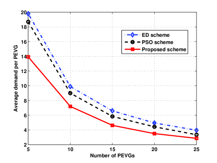
Figure 8: Effect of the number of PEVGs in the network on the average demand of a PEVG.

In Fig. 9, we show the average utility achieved by all three schemes as a function of the number of PEVGs. In this figure, we can see that the average utility per PEVG decreases as $N$ increases for all three schemes. This is due to the fact that the benefit extracted by each PEVG decreases as more PEVGs share the fixed available energy from the grid. However, importantly, Fig. 9 shows that the proposed scheme has a performance advantage at all network sizes which is, on the average, $1.6$ times that of the PSO scheme. When compared to the ED scheme, the proposed scheme shows significant improvements for all network sizes, reaching an improvement of up to $3.5$ times over the ED scheme for $N=25$ PEVGs.

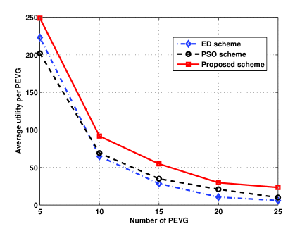
Figure 9: Effect of the number of PEVGs in the network on the average utility per PEVG.

In Fig. 10, we assess the average demand of energy per PEVG in a time-varying environment. Here, the state transition of the variable $C_{t}$ in (34) is modeled as an independent stochastic process [34], due to the random changes in traffic conditions and grid energy from one time instant to another [40]. The state of available energy at the grid at any time $t$ is assumed to be a uniformly distributed random variable in the range [$0.5,1.5$] times the average available energy [40]. The capacity of the PEVGs $b_{n}^{t}~{}\forall n\in\mathcal{N}~{}\text{at}~{}t=1,2,.....,T$, is assumed to be a uniformly distributed random variable in the range [$0.5,1.5$] times the average battery capacity  [40]. Assuming that the traffic conditions in any PEVG changes every $30$ minutes, we have run independent simulations for allocating energy to the PEVGs for eight time slots in peak hours (from 12 pm to 4 pm). The average available energy in the grid is $66$ MWh (assuming a range from $33$ to $99$ MWh), and the variation of energy across time slots is modeled by a uniformly distributed random variable between $0.5$ and $1.5$ of this amount [40]. Similarly, the random variation in PEVGs’ capacity at different time slots is captured assuming a maximum of $55$ MWh (for $1000$ PEVs in a PEVG) and a minimum of $9.9$ MWh (for $300$ PEVs) [20].

In Fig. 10 it is shown that the demand of any PEVG varies across time slots due to variation in both satisfaction parameters of the PEVGs and the available energy. However, the minimum energy demand by any PEVG is always well above its minimum battery requirement. For example, the minimum demand by PEVG $4$ is $5.5$ MWh in time slot $1$, which exceeds the minimum battery requirement of a mid-size car, assuming $1000$ PEVs are in that PEVG [41].

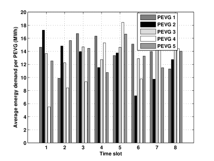
Figure 10: Average demands of the PEVGs at the GSE for the proposed scheme in a dynamic environment.

The change of utility per PEVG in a time-varying environment is shown in Fig. 11 for the proposed, PSO and ED schemes. Fig. 11 shows that the team optimal solution achieved by the proposed scheme leads to an improved average utility for the PEVG when compared to the PSO and ED schemes. However, the improvement varies across time slots due to variations in available energy and the number of PEVs in the smart grid network. As shown in Fig. 11, the average utility achieved per PEVG by our proposed scheme is, on the average, $1.6$ times the utility achieved by the PSO scheme and $3.8$ times that achieved by the ED scheme.

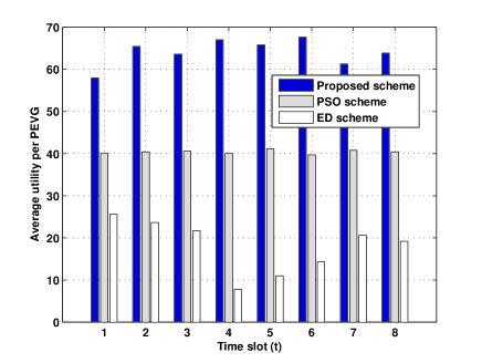
Figure 11: Comparison of the average utility per PEVG in the dynamic case.

VII Conclusions

In this paper, we have formulated a noncooperatibe Stackelberg game to study the problem of energy trading between an SG and a number of PEV groups. In this game, the SG chooses its price to maximize its revenue whereas the PEVGs strategically choose the amounts of energy they wish to buy from the grid so as to optimize a tradeoff between the benefit of battery charging and associated costs. We have studied the properties of this solution and we have shown that this game admits a socially optimal generalized Stackelberg equilibrium. We have also extended and analyzed the proposed game in a time-varying environment. To reach the equilibrium of the game, we have proposed a novel algorithm that can be adopted by the PEVGs, in a distributed manner. Simulation results have shown that the proposed approach yields improved performance gains, in terms of the average utility per PEVG, compared to a particle swarm optimization and an equal distribution scheme. Several future extensions can be foreseen for this work, such as handling rapidly changing dynamics or determining the optimal deployment of charging stations depending on a variety of factors such as the parking duration, battery state, and the location of the vehicles.

Wayes Tushar received his B.Sc. degree in Electrical and Electronic Engineering from Bangladesh University of Engineering and Technology in 2007. He is currently a Ph.D. Candidate at the Research School of Engineering in Australian National University (ANU). From May 2011 to June 2011 he was a visiting student research collaborator at the School of Engineering and Applied Science in Princeton University. He received the best student paper award in the Australian Communications Theory Workshop in 2012. His research interests include smart grid systems, game theory and signal processing.

Walid Saad received his B.E. from the Lebanese University in 2004, his M.E. in Computer and Communications Engineering from the American University of Beirut in 2007, and his Ph.D degree from the University of Oslo in 2010. From August 2008 till July 2009 he was a visiting scholar at the Coordinated Science Laboratory at the University of Illinois at Urbana Champaign. From January 2011 till July 2011, he was a Postdoctoral Research Associate at the Electrical Engineering Department at Princeton University. Currently, he is an Assistant Professor at the Electrical and Computer Engineering Department at the University of Miami. His research interests span the areas of game theory, wireless networks, and the smart grid. He was the first author of the papers that received the Best Paper Award at the 7th International Symposium on Modeling and Optimization in Mobile, Ad Hoc and Wireless Networks (WiOpt), in June 2009 and at the 5th International Conference on Internet Monitoring and Protection (ICIMP) in May 2010. He is a co-author of the paper that won the best paper award at the IEEE Wireless Communications and Networking Conference (WCNC) in 2012.

H. Vincent Poor (S’72, M’77, SM’82, F’87) received the Ph.D. degree in EECS from Princeton University in 1977. From 1977 until 1990, he was on the faculty of the University of Illinois at Urbana-Champaign. Since 1990 he has been on the faculty at Princeton, where he is the Michael Henry Strater University Professor of Electrical Engineering and Dean of the School of Engineering and Applied Science. Dr. Poor’s research interests are in the areas of stochastic analysis, statistical signal processing, and information theory, and their applications in wireless networks and related fields such as social networks and smart grid. Among his publications in these areas are the recent books Classical, Semi-classical and Quantum Noise (Springer, 2012) and Smart Grid Communications and Networking (Cambridge University Press, 2012). Dr. Poor is a member of the National Academy of Engineering and the National Academy of Sciences, a Fellow of the American Academy of Arts and Sciences, and an International Fellow of the Royal Academy of Engineering (U.K.). He is also a Fellow of the Institute of Mathematical Statistics, the Acoustical Society of America, and other organizations. In 1990, he served as President of the IEEE Information Theory Society, and in 2004-07 he served as the Editor-in-Chief of the IEEE Transactions on Information Theory. He received a Guggenheim Fellowship in 2002 and the IEEE Education Medal in 2005. Recent recognition of his work includes the 2010 IET Ambrose Fleming Medal, the 2011 IEEE Eric E. Sumner Award, the 2011 Society Award of the IEEE Signal Processing Society, and honorary doctorates from Aalborg University, the Hong Kong University of Science and Technology and the University of Edinburgh.

David Smith is a Senior Researcher at National ICT Australia (NICTA) and is an adjunct Fellow with the Australian National University (ANU), and has been with NICTA and the ANU since 2004. He received the B.E. degree in Electrical Engineering from the University of N.S.W. Australia in 1997, and while studying toward this degree he was on a CO-OP scholarship. He obtained an M.E. (research) degree in 2001 and a Ph.D. in 2004 both from the University of Technology, Sydney (UTS), and both in Telecommunications Engineering. His research interests are in technology and systems for wireless body area networks; game theory for distributed networks; mesh networks; radio propagation and electromagnetic modeling; MIMO wireless systems; coherent and non-coherent space-time coding; and antenna design, including the design of smart antennas. He also has research interest in optimization for smart grid. He has also had a variety of industry experience in electrical engineering; telecommunications planning; radio frequency, optoelectronic and electronic communications design and integration. He has published numerous technical refereed papers and made various contributions to IEEE standardization activity; and has received a best paper award as first author at 1st International Symposium on Applied Sciences on Biomedical and Communication Technologies, 2008, (ISABEL ’08); and has two other conference best paper awards, one as first author and another as co-author.

References

- [1] P. Bauer, Y. Zhou, J. Doppler, and N. Stembridge, “Charging of electric vehicles and impact on the grid,” in Proc. International Symposium MECHATRONIKA, Trencianske Teplice, Jun. 2010.
- [2] N. Rotering and M. Ilic, “Optimal charge control of plug-in hybrid electric vehicles in deregulated electricity markets,” IEEE Trans. Power Syst., vol. 26, pp. 1021–1029, 2011.
- [3] A. M. Foley, I. J. Winning, and B. P. O. Gallachoir, “State-of-the-art in electric vehicle charging infrastructure,” in Proc. IEEE Vehicle Power and Propulsion Conference, Lille, France, Sep. 2010.
- [4] P. Samadi, A. H. Mohsenian-Rad, R. Schober, V. W. S. Wong, and J. Jatskevich, “Optimal real-time pricing algorithm based on utility maximization for smart grid,” in Proc. IEEE International Conference on Smart Grid Communication, Gaithersburg, MD, Nov. 2010.
- [5] C. Wu, H. Mohsenian-Rad, and J. Huang, “Vehicle-to-aggregator interaction game,” IEEE Trans. Smart Grid, vol. 3, pp. 434–442, Mar. 2012.
- [6] F. Pan, R. Bent, A. Bercheid, and D. Izraelevitz, “Locating PHEV exchange stations in V2G,” in Proc. International Conference on Smart Grid Communications, Gaithersburg, MD, Nov. 2010.
- [7] S. Sojoudi and S. H. Low, “Optimal charging of plug-in hybrid electric vehicles in smart grid,” in Proc. IEEE Power and Energy Society (PES) General Meeting, Detroit, MI, Jul. 2011.
- [8] K. Turitsyn, N. Sinitsyn, S. Backhaus, and M. Chertkov, “Robust broadcast-communication control of electric vehicle charging,” in Proc. IEEE International Conference on Smart Grid Communications, Gaithersburg, MD, Oct. 2010.
- [9] K. C. Nyns, E. Haesen, and J. Driesen, “The impact of charging plug-in hybrid electric vehicles on a residential distribution grid,” IEEE Trans. Power Syst., vol. 25, pp. 371–380, 2010.
- [10] S. Ka̧birch, A. Schmitt, M. Winter, and J. Heuer, “Interconnections and communications of electric vehicles and smart grids,” in Proc. IEEE International Conference on Smart Grid Communications, Gaithersburg, MD, Oct. 2010.
- [11] R. Couillet, S. Perlaza, H. Tembine, and M. Debbah, “Electrical vehicles in the smart grid: A mean field game analysis,” IEEE J. Select. Areas Commun., vol. 30, no. 6, pp. 1086 –1096, july 2012.
- [12] W. Su and M. Y. Chow, “Performance evaluation of a PHEV parking station using particle swarm optimization,” in Proc. IEEE Power and Energy Society General Meeting, Detroit, MI, Jul. 2011.
- [13] C. Hutson, G. K. Venayagamoorthy, and K. A. Corzine, “Intelligent scheduling of hybrid and electric vehicle storage capacity in a parking lot for profit maximization in grid power transactions,” in Proc. IEEE Energy Conference, Atlanta, GA, Nov. 2008.
- [14] A. Foley, B. Tyther, and B. Ó. Gallachóir, “Modelling of impacts of electric vehicle charging in the single electricity market,” in Proc. Dubrovnik Conference on Sustainable Development of Energy, Water and Environment System, Dubrovnik, Croatia, Sep. 2011.
- [15] A. Foley, H. Daly, E. McKeogh, and B. Ó. Gallachóir, “Quantifying the energy & carbon emissions implications of a 10 percent electric vehicles target,” in Proc. International Energy WOrkshop, Stockholm, Sweden, Jun. 2010.
- [16] A. Foley, P. G. Leahy, B. Ó. Gallachóir, and E. McKeogh, “Electric vehicles and energy storage: A case study on Ireland,” in Proc. IEEE Electric Vehicle Power and Propulsion Conference, Dearborn, MI, Sep. 2009.
- [17] P. Palensky and D. Dietrich, “Demand side management: demand response, intelligent energy systems, and smart loads,” IEEE Trans. Ind. Informat., vol. 7, pp. 381–388, 2011.
- [18] W. Zhenpo and L. Peng, “Analysis on storage power of electric vehicle charging station,” in Proc. Asia-Pacific Power and Energy Engineering Conference, Chengdu, China, Mar. 2010.
- [19] P. Stroehle, S. Becher, S. Lamparter, A. Schuller, and C. Weinhardt, “The impact of charging strategies for electric vehicles on power distribution networks,” in Proc. International Conference on the European Energy Market, Zagreb, Croatia, May 2011.
- [20] M. D. Galus and G. Anderson, “Demand management of grid connected plug-in hybrid electric vehicles (PHEV),” in Proc. IEEE Energy 2030 Conference, Atlanta, GA, Feb. 2008.
- [21] W. H. Lin, “A Gaussian maximum likelihood formulation for short-term forecasting of traffic flow,” in Proc. IEEE Intelligent Transportation Systems Conference, Oakland, CA, Aug. 2001.
- [22] T. Başar and G. J. Olsder, Dynamic Noncooperative Game Theory. Philadelphia, PA: SIAM, 1999.
- [23] M. Fahrioglu, M. Fern, and F. Alvarado, “Designing cost effective demand management contracts using game theory,” in Proc. IEEE Power Eng. Soc. 1999 Winter Meeting, New York, NY, Jan. 1999.
- [24] F. Facchinei and C. Kanzow, “Generalized Nash equilibrium problems,” 4OR, vol. 5, pp. 173–210, Mar. 2007.
- [25] D. Ardagna, B. Panicucci, and M. Passacantando, “A game theoretic formulation of the service provisioning problem in cloud systems,” in Proc. International World Wide Web Conference, Hyderabad, India, Apr. 2011.
- [26] T. Başar and R. Srikant, “Revenue maximizing pricing and capacity expansion in a many-users regime,” in Proc. IEEE International Conference on Computer Communications, New York, NY, Jun. 2002.
- [27] D. Bertsekas, Nonlinear Programming. Belmont, MA: Athena Scientific, 1995.
- [28] M. V. Solodov and B. F. Svaiter, “A new projection method for variational inequality problems,” SIAM J. Control Optim., vol. 37, pp. 765–776, 1999.
- [29] F. Tinti, “Numerical solution for pseudo monotone variational inequality problems by extra gradient methods,” Website, 2003, http://dm.unife.it/~tinti/Software/Extragradient/methods/vipsegm.pdf.
- [30] L. Armijo, “Minimization of functions having continuous partial derivatives,” Pacific Journal of Mathematics, 1966.
- [31] A. Nedic and U. V. Shanbhag, “Lecture 21: Algorithms for monotone vis projection methods,” Website, 2008, https://netfiles.uiuc.edu/angelia/www/ie598ns_lect21_2.pdf.
- [32] P. Y. Nie, L. H. Chen, and M. Fukushima, “Dynamic programming approach to discrete time dynamic feedback Stackelberg games with independent and dependent followers,” Elsevier European Journal of Operational Research, vol. 169, pp. 310–328, 2006.
- [33] O. Derin and A. Ferrante, “Scheduling energy consumption with local renewable micro-generation and dynamic electricity prices,” in Proc. of The First Workshop on Green and Smart Embedded System Technology: Infrastructures, methods and Tools, Stockholm, Sweden, Apr. 2010.
- [34] K. Staňkovà and B. D. Schutter, “Stackelberg equilibria for discrete-time dynamic games part II: Stochastic games with deterministic information structure,” in Proc. International Conference on Networking, Sensing and Control, Deift, the Netherlands, Apr. 2011.
- [35] B. Tolwinski, “A Stackelberg solution of dynamic games,” IEEE Trans. Automat. Contr., vol. AC-28, pp. 85–93, 1983.
- [36] C. Silva, M. Ross, and T. Farias, “Evaluation of energy consumption, emissions and cost of plug-in hybrid vehicles,” Elsvier Energy Conversion and Management, vol. 50, pp. 1635–1643, Jul. 2009.
- [37] T. Motors, “Roadster innovations: Motor,” Website, Feb. 2011, http://www.teslamotors.com/roadster/technology/motor.
- [38] C. H. Chen, S. Y. Lin, H. C. Chang, and C. C. Lo, “On the design and development of a novel real-time transaction price estimation system,” Advanced Material Research, vol. 393-395, pp. 213–216, Nov. 2011.
- [39] C. C. Chan and Y. S. Wong, “Electric vehicles charge forward,” IEEE Power and Energy Magazine, vol. 2, pp. 24–33, 2004.
- [40] F. Pan, R. Bent, A. Bercheid, and D. Izraelevitz, “Locating PHEV exchange stations in V2G,” in Proc. IEEE First International Conference on Smart Grid Communication, Gaithersburg, MD, Oct. 2010.
- [41] A. Roussean, N. Shidore, R. Carlson, and V. Frevermuth, “Research on PHEV battery requirements and evaluation of early prototypes,” in Proc. IEEE Advanced Automotive Battey Conference, Long Beach, CA, May 2007.