Special transformations for pentamode acoustic cloaking

Abstract

The acoustic cloaking theory of NorrisNorris (2008) permits considerable freedom in choosing the transformation $f$ from physical to virtual space. The standard process for defining cloak materials is to first define $f$ and then evaluate whether the materials are practically realizable. In this paper, this process is inverted by defining desirable material properties and then deriving the appropriate transformations which guarantee the cloaking effect. Transformations are derived which result in acoustic cloaks with special properties such as 1) constant density 2) constant radial stiffness 3) constant tangential stiffness 4) power-law density 5) power-law radial stiffness 6) power-law tangential stiffness. 7) minimal elastic anisotropy.

1 Introduction

Acoustic cloaking refers to making an object invisible to sound waves. This is achieved by enclosing the object of interest with an acoustic cloak which guides waves around the object. The cloak leaves the wave-field outside the cloak indistinguishable from the wave-field without the object present. The phenomenon of cloaking is not restricted to acoustics but can occur for different types of waves such as electromagnetic waves Pendry and Li (2008), elastic waves Norris and Shuvalov (2011), and in a more exotic example, quantum mechanical systems Zhang et al. (2008). We restrict our attention here to acoustic cloaking, and specifically pentamode acoustic cloaking for which the density is isotropic. The reader is referred to the review articles by Bryan and LeiseBryan and Leise (2010) and Greenleaf et al.Greenleaf et al. (2009) for a comprehensive review of different types of cloaking, its historical development and relation to previous work in inverse problems Greenleaf et al. (2003). A review dedicated to acoustic cloaking and transformation acoustics is provided by Chen and Chan Chen and Chan (2010).

Initial work in acoustic cloaking Cummer and Schurig (2007); Chen and Chan (2007); Cummer et al. (2008) was based on transformation optics as developed by Pendry et al. Pendry et al. (2006). Cummer et al. Cummer and Schurig (2007) mapped the 2D acoustic equations in a fluid to the single polarization Maxwell’s equations, while Chen et al.Chen and Chan (2007) mapped the 3D acoustic equation to the direct current conductivity equation in 3D. Cummer et al.Cummer et al. (2008) derived a formulation for 3D acoustic cloaking starting from scattering theory. These formulations achieved acoustic cloaking using anisotropic density and isotropic stiffness. Norris Norris (2008) provided a formulation of acoustic cloaking which using both anisotropic inertia and stiffness, and as a special case, derived a formulation using isotropic density and anisotropic stiffness.

The acoustic cloaking theory of NorrisNorris (2008) involves mapping the physical space to the virtual space using the transformation $f$ as illustrated in Figure 1. The material properties of the cloak can be obtained by choosing the transformation $f$ and using eqs. (3) to compute the material properties. In practice, however, the properties obtained may not be useful because they are unattainable. In this paper, we derive special forms of $f$ which may result in physically realizable cloaking metamaterials, which are composite materials whose macroscopic acoustic properties are controlled by engineering their microstructure. The design and fabrication of such acoustic metamaterials is possible because of recent advances in material science and engineering. Cloaking metamaterials may have spatially varying anisotropic density and stiffness. We restrict our attention here to spatially varying material properties with isotropic density and anisotropic stiffness because NorrisNorris (2008) showed that anisotropic density implies that the acoustic cloak has infinite mass. He presented an alternative acoustic cloaking formulation involving pentamode materials which have isotropic density and a special type of anisotropic stiffness. Since cloaking is achieved with anisotropic stiffness as opposed to density, it is expected to have frequency independent behavior in theory.

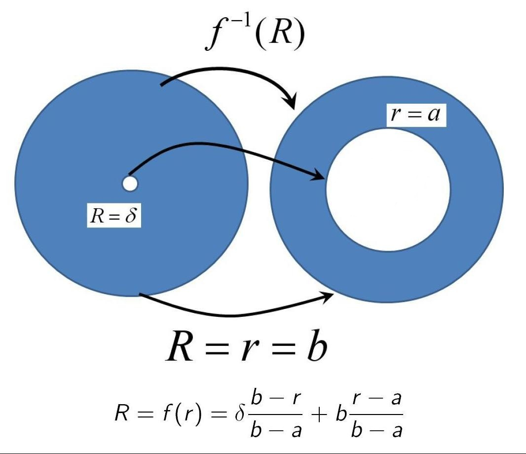
Figure 1: The transformation $f$ from physical space (right) to virtual space (left). The particular mapping shown is the linear mapping of eq. (2a).

In practice, however, the behavior is expected to be only extremely wideband or weakly frequency dependent because of frequency limitations arising from:

• the size of the virtual cloak radius $\delta$ as compared to the wave-length of the incident acoustic wave $\lambda$. Cloaking is ineffective for incident acoustic waves whose wavelength is of the same order as the virtual cloak radius $\delta$.

• the length scale of periodic structures present in the composite material used to fabricate the pentamode material.

• an intrinsic frequency dependence in the properties of the composite material.

The paper is organized as follows. Section 2 provides a short review of the pentamode acoustic cloaking theoryNorris (2008). Next, in §3, we derive transformations $f$ which yield specialized spatial distributions of material properties, namely, 1) constant density 2) constant radial stiffness 3) constant tangential stiffness and explain the wave-propagation with ray-tracing. Such distributions may be simple to manufacture and may also help in evaluating the feasibility of manufacturing material properties on Ashby charts, as inUrzhumov et al. (2010). We note that in related work, CummerCummer et al. (2009) has derived transformations for electromagnetic cloaking which yield constant magnetic permittivity $\epsilon_{\phi}$. In §4 we derive transformations which yield 1) power-law density 2) power-law radial stiffness 3) power-law tangential stiffness. In §5, we derive a distribution of elastic properties that minimizes the elastic anisotropy.

2 Review of acoustic cloaking using pentamode materials

Acoustic cloaking relies on a transformation from an undeformed or original domain $\Omega$ to a current (deformed) domain $\omega$ which is given by the point-wise deformation ${\mbox{\boldmath$\displaystyle\mathbf{X}$}}\in\Omega$ $\rightarrow$ ${\mbox{\boldmath$\displaystyle\mathbf{x}$}}\in\omega$. Using notation from the theory of finite elasticity, the deformation gradient is defined ${\mbox{\boldmath$\displaystyle\mathbf{F}$}}=\nabla_{X}{\mbox{\boldmath$\displaystyle\mathbf{x}$}}$, or in component form $F_{iI}=\partial x_{i}/\partial X_{I}$. The Jacobian of the deformation is $J=\det{\boldsymbol{F}}$, or in terms of volume elements in the two configurations, $J=\operatorname{d}v/\operatorname{d}V$. The polar decomposition is ${\boldsymbol{F}}={\boldsymbol{V}}{\boldsymbol{R}}$, where ${\boldsymbol{R}}$ is proper orthogonal (${\boldsymbol{R}}{\boldsymbol{R}}^{t}={\boldsymbol{R}}^{t}{\boldsymbol{R}}={\boldsymbol{I}}$, $\det{\boldsymbol{R}}=1$) and the left stretch tensor ${\boldsymbol{V}}$ is the positive definite solution of ${\boldsymbol{V}}^{2}={\boldsymbol{B}}$ where ${\boldsymbol{B}}$ is the left Cauchy-Green or Finger tensor ${\boldsymbol{B}}={\boldsymbol{F}}{\boldsymbol{F}}^{t}$.

For a given transformation the cloaking material is not uniqueNorris (2008). For instance, the inertial cloak (Norris, 2008, eq. (2.8)) is defined by the density tensor ${\boldsymbol{\rho}}=\rho_{0}J{\mbox{\boldmath$\displaystyle\mathbf{B}$}}^{-1}$ and bulk modulus $K=K_{0}J$. At the other end of the spectrum of possible materials is the pentamode cloak with isotropic density, which can be chosen if the deformation satisfies the property(Norris, 2008, Lemma 4.3) that there is a function $h({\mbox{\boldmath$\displaystyle\mathbf{x}$}})$ for which $\operatorname{div}h{\mbox{\boldmath$\displaystyle\mathbf{V}$}}=0$. This is the case for radially symmetric deformations in 2D and 3D, the cylinder and sphere, respectively. The pentamode material is then(Norris, 2008, eq. (4.8)) $\rho=\rho_{0}J^{-1}$, $K=K_{0}J$, ${\mbox{\boldmath$\displaystyle\mathbf{S}$}}=J^{-1}{\mbox{\boldmath$\displaystyle\mathbf{V}$}}$, where the fourth order elasticity tensor is ${\mbox{\boldmath$\displaystyle\mathbf{C}$}}=K{\mbox{\boldmath$\displaystyle\mathbf{S}$}}\otimes{\mbox{\boldmath$\displaystyle\mathbf{S}$}}$.

Radially symmetric deformations in 2D and 3D are defined by $R^{-1}{\mbox{\boldmath$\displaystyle\mathbf{X}$}}=r^{-1}{\mbox{\boldmath$\displaystyle\mathbf{x}$}}$ where $R=|{\mbox{\boldmath$\displaystyle\mathbf{X}$}}|$, $r=|{\mbox{\boldmath$\displaystyle\mathbf{x}$}}|$. If we let $R=f(r)$, then the inverse mapping is defined as ${\mbox{\boldmath$\displaystyle\mathbf{X}$}}=f(r)r^{-1}{\mbox{\boldmath$\displaystyle\mathbf{x}$}}$. In this case we can identify a “radial bulk modulus” and an orthogonal bulk modulus

$$K_{r}\equiv C_{rrrr}=K_{0}J^{-1}B_{rr},\quad K_{\perp}\equiv K_{0}J^{-1}B_{\theta\theta},$$ (1)

where $\theta$ denotes a direction orthogonal to the radial direction.

The requirements on the transformation generator $f(r)$ admit an infinity of functions. In this paper, we will take advantage of this fact to design transformations which result in desirable material properties. One familiar transformation, used frequently in acoustic cloaking work, is shown in Figure 1. Some examples from the infinite family of permissible transformations are:

$$R=f(r)=\begin{cases}\big{(}\frac{b-\delta}{b-a}\big{)}r-b\big{(}\frac{a-\delta}{b-a}\big{)},&(a)\\ b\,\big{(}\frac{r}{b}\big{)}^{\frac{\ln(b/\delta)}{\ln(b/a)}},&(b)\\ \bigg{[}\bigg{(}\frac{b^{d}-\delta^{d}}{b^{d}-a^{d}}\bigg{)}r^{d}-\bigg{(}\frac{a^{d}-\delta^{d}}{b^{d}-a^{d}}\bigg{)}b^{d}\bigg{]}^{\frac{1}{d}}.&(c)\end{cases}$$ (2)

where $b$, $a$ and $\delta$ are the outer radius of the cloak, the inner radius of the cloak, and the virtual cloak radius, as shown in Figure 1. The linear transformation (2a) is known as the KSVW mapping for the paper Kohn et al. (2008) in which it was first used extensively in this form. Figure 2(a) shows rays passing through a KSVW cloak. The power law mapping (2b) yields constant $\rho_{r}$ for the inertial cloak and constant $K_{r}$ for the pentamode cloak in 2D. As we will see below, the transformation (2c) yields constant $K$ for the inertial cloak or constant $\rho$ for the pentamode cloak.

3 Transformations yielding constant material property distributions

In this section we determine the transformations $f$ that yield constant spatial distributions of material properties. We consider a constant distribution of $\rho$ in §3.1, constant $K_{r}$ in §3.2, and constant $K_{\perp}$ in §3.3, respectively. Both 2D and 3D cases are considered. The conditions for feasibility are summarized in Table 1.

Constant	d=2	d=3	Conditions other than $\rho_{0},K_{0}>0$
$\rho$	✓	✓	$\rho_{c}>\rho_{0}$
$K_{r}$	✓	✓	Conditional in 3D, $K_{r}<\frac{K_{0}\delta}{a}$, $K_{r}>0$
$K_{\perp}$	✓	✓	Conditional in 3D, $K_{0}<K_{\perp}$

Table 1: Feasibility of constant material properties in 2D $(d=2)$ and 3D $(d=3)$.

The density $\rho$ (isotropic), the radial stiffness $K_{r}$, and the tangential stiffness $K_{\perp}$ for a pentamode cloak surrounded by an anisotropic fluid with density $\rho_{0}$ and bulk modulus $K_{0}$ satisfy the following relations:

$$K_{r}(r)=K_{0}\frac{1}{f^{\prime}}\Big{(}\frac{f}{r}\Big{)}^{d-1},\ \ K_{\perp}(r)=K_{0}f^{\prime}\Big{(}\frac{f}{r}\Big{)}^{d-3},$$ (3)

$$\qquad\qquad\rho(r)={\rho_{0}}f^{\prime}\Big{(}\frac{f}{r}\Big{)}^{d-1},$$

Our procedure to determine $f$ consists of treating eqs. (3) as differential equations for $f$ with the material properties ($\rho,K_{r},K_{\perp}$) known. Having determined $f$ we will prove that it satisfies the necessary conditions $f>0,f^{\prime}>0$ for $r\in[a,b]$, the existence of $b$ such that $f(b)=b$, and the existence of $\delta$ such that $f(a)=\delta<<a$.

We remark that eqs. (3) are consistent with the connection between the three parameters which is independent of the transformation:

$$K_{0}^{-d}K_{r}K^{d-1}_{\perp}=(\rho/\rho_{0})^{d-2}.$$ (4)

Equations (3) also imply that at the edge of the cloak, the cloak is impedance matched in the radial direction but not in the tangential direction:

$$Z_{r}(r) \equiv\sqrt{K_{r}\rho}\ \ \Rightarrow\ \ Z_{r}(b)=\sqrt{K_{0}\rho_{0}}\equiv Z_{0}\,,$$ (5)

$$Z_{\perp}(r) \equiv\sqrt{K_{\perp}\rho}\ \ \Rightarrow\ \ Z_{\perp}(b)=Z_{0}{f^{\prime}}(b).$$

In contrast, at the edge of the cloak, the wave speeds are matched in the tangential direction, but not in the radial direction:

$$c_{r}(r) \equiv\sqrt{{K_{r}}/{\rho}}\ \ \Rightarrow\ \ c_{r}(b)={c_{0}}/{f^{\prime}}(b),$$ (6)

$$c_{\perp}(r) \equiv\sqrt{{K_{\perp}}/{\rho}}\ \ \Rightarrow\ \ c_{\perp}(b)=c_{0}.$$

3.1 Transformations yielding constant cloak density $\rho$

We assume that we are given the cloak geometry $b>a>0$, and using equation (3) and $\rho(r)=\rho_{c}$, a constant, we determine $f$ and prove that $f>0,f^{\prime}>0$ for $r\in\,(a,b)$. Solving (3) for $f$ yields

$$f=\big{[}b^{d}+\frac{\rho_{c}}{\rho_{0}}\big{(}r^{d}-b^{d}\big{)}\big{]}^{1/d},$$ (7)

and differentiating implies $f^{\prime}>0$ for $\rho_{c}>0$, showing that $f$ is monotonically increasing. Since $f(a)=\delta>0$, $f>0\in(a,b)$. Enforcing $\delta=f(a)<a$ yields $\rho_{c}>\rho_{o}$. This result makes physical sense because the deformation $f^{-1}$ compresses the volume of fluid into a smaller volume. $K_{r},K_{\perp}$ are determined by using $f$ in equation (3) and are given by:

$$K_{r}=K_{0}\frac{\rho_{0}}{\rho_{c}}\bigg{(}\frac{f}{r}\bigg{)}^{2(d-1)},\ \ K_{\perp}=K_{0}\frac{\rho_{c}}{\rho_{0}}\bigg{(}\frac{r}{f}\bigg{)}^{2}.$$ (8)

Similarly $\delta$ and its sensitivity can be determined by

$$\delta=\big{[}b^{d}+\frac{\rho_{c}}{\rho_{0}}\big{(}a^{d}-b^{d}\big{)}\big{]}^{1/d},\ \ \frac{\partial\delta}{\partial\rho_{c}}=\frac{a^{d}-b^{d}}{\rho_{0}{d}\delta^{d-1}}{<0}.$$ (9)

Finally, note that, $K_{r}\propto\delta^{2(d-1)}\text{ and }K_{\perp}\propto{\delta^{-2}}$ In 3D this implies a very strong decrease in $K_{r}$ with $\delta$.

We note that rays in the cloak are straight lines in deformed spaceNorris (2008). This allows us to trace the rays for the constant density cloak by deforming the straight rays corresponding to a plane wave traveling through a homogeneous medium by the inverse transformation $f^{-1}$. Ray-tracing results are shown in Figure 2(b), from which we can see that the rays curve gently in the outer region of the cloak and sharply close to the inner radius. In our experience, the smooth nature of this propagation makes it easy for this to be simulated with standard linear finite elements .

(a) KSVW cloak

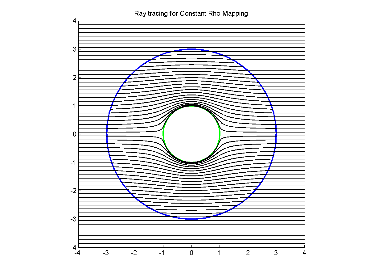
(b) Constant density cloak

(c) Constant stiffness cloak

(d) Cloak with optimal anisotropy

Figure 2: Rays for KSVW, constant density, constant stiffness, and optimal anisotropy cloaks in 2D, $a=1,b=3$.

(a) Initial propagation.

(b) Complete propagation.

Figure 3: Rays for power law $K_{r}$, with parameters $a=1,b=3$, $\alpha=3$.

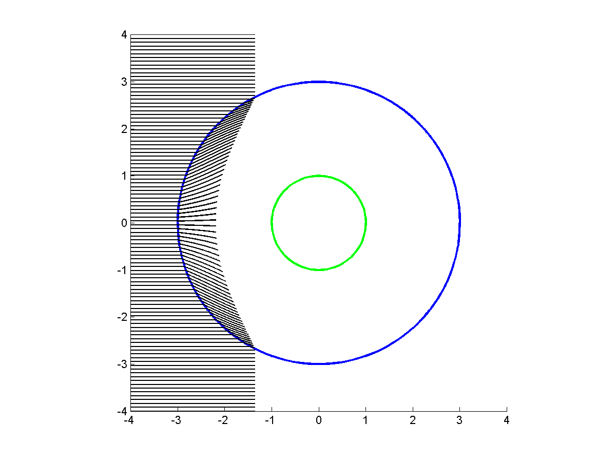
(a) Initial propagation.

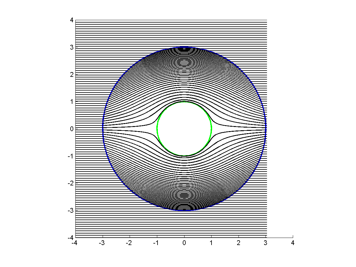
(b) Complete propagation.

Figure 4: Rays for power law $\rho$, with parameters $a=1$, $b=3$, $\alpha=3$.

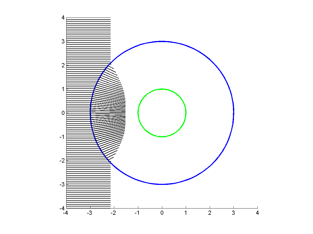
(a) Initial propagation I.

(b) Initial propagation II.

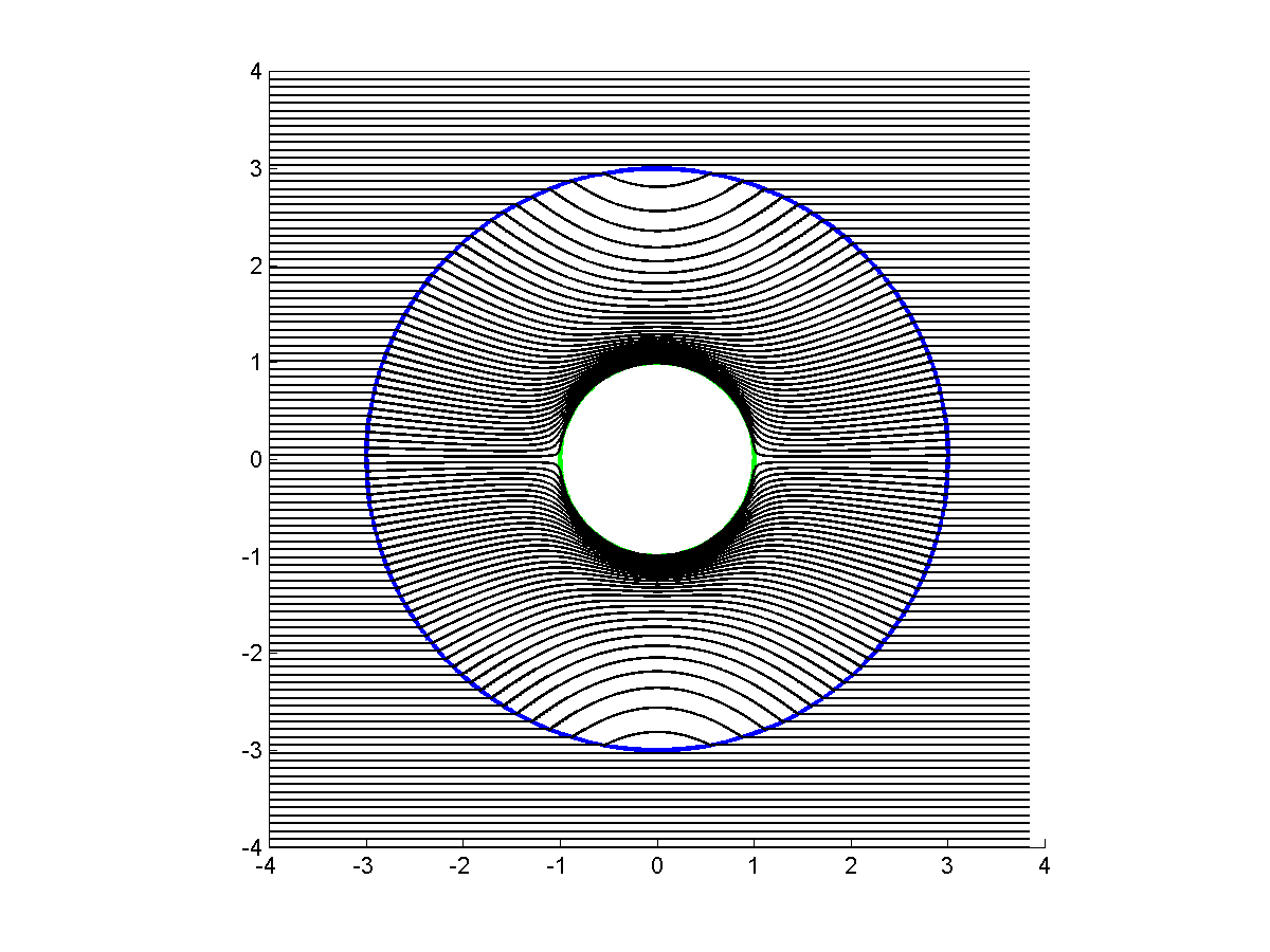
(c) Complete propagation.

Figure 5: Rays for power law $\rho$, with parameters $a=1$, $b=3$, $\alpha=-3$.

(a) Initial propagation.

(b) Rays converging.

(c) Complete propagation.

Figure 6: Rays for an acoustic concentrator $f(r)=b(r/b)^{1/10}$.

3.2 Transformations yielding constant radial stiffness $K_{r}$

We formulate the problem by assuming that we are given $a>\delta>0$ and $K_{r}$ constant. As before, start with the expression for $K_{r}$ from equation (3), and treat it as an ordinary differential equation for $f$ and get

$$\int{\frac{f^{\prime}}{f^{d-1}}dr}={\frac{K_{0}}{K_{r}}\int\frac{dr}{r^{d-1}}}.$$ (10)

The solution is different for 2D and 3D and is determined separately in the next two subsections.

3.2.1 Transformation yielding constant $K_{r}$ in 2D

The transformation $f$ in 2D can be determined by solving equation (10) to get

$$f=b\,\big{(}\frac{r}{b}\big{)}^{\frac{K_{0}}{K_{r}}}>0,\ \ f^{\prime}=\frac{K_{0}}{K_{r}}\frac{f}{r}>0.$$ (11)

The cloak parameters then follow from eq.  (3) as

$$\rho=\rho_{0}\frac{K_{0}}{K_{r}}\big{(}\frac{r}{b}\big{)}^{2(\frac{K_{0}}{K_{r}}-1)},\ \ K_{r}=\frac{K^{2}_{0}}{K_{\perp}}=K_{0}\frac{\ln{a/b}}{\ln{\delta/b}},$$ (12)

$$\quad\delta=a\,\big{(}\frac{a}{b}\big{)}^{\frac{K_{0}}{K_{r}}-1},\ \ \frac{\partial\delta}{\partial K_{r}}=\frac{\delta}{K_{r}}\ln\big{(}\frac{b}{\delta}\big{)}>0.$$

We prove that given $a>\delta>0$, it is possible to find $b$ such that $b>a>\delta>0\,\forall\,\,K_{r}=\text{constant}>0,\,K_{r}{\neq}K_{0}$. Since $\frac{\delta}{a}<1$ and $a<b$, the exponent $\frac{K_{0}}{K_{r}}-1$ in eq. (12) must be positive to ensure $b>a$. i.e. $0<K_{r}<K_{0}$ must hold for constant $K_{r}$ cloaks in 2D. This shows that the cloak outer radius is greater than the inner radius, making the cloak physically realistic.

This case is of interest because the only parameter that varies with $r$ is the density. At the outer radius $\rho(b)=\rho_{0}\frac{K_{0}}{K_{r}}>\rho_{0}$, and the value at the inner radius is $\rho(a)=\rho(b)(\delta/a)^{2}$.

The rays for a constant $K_{r}$ cloak in 2D are shown in Figure 2(c). Unlike the rays for the constant density cloak shown in Figure 2(b), the rays for constant stiffness curve sharply at the outer surface of the cloak. In our experience, the propagation of waves near the surface is extremely hard to capture with standard linear, time-domain, finite elements, possibly due to sharp change in the direction of propagation. The required element density is in the order of hundreds of elements per shortest wavelength. This is contrast to the rule of thumb in transient, explicit finite element analysis in which typically sixteen elements per shortest wavelength are used.

3.2.2 Transformation yielding constant $K_{r}$ in 3D

Treating equation (10) with $d=3$ as a differential equation for $f$ with $K_{r}$ known and constant, gives

$$f=\big{[}\frac{1}{b}+\frac{K_{0}}{K_{r}}\Big{(}\frac{1}{r}-\frac{1}{b}\Big{)}\Big{]}^{-1}\ \text{ and }\ f^{\prime}=\frac{K_{0}}{K_{r}}\big{(}\frac{f}{r}\big{)}^{2}>0.$$ (13)

Using the above definition of $f$ in eq. (3) we get

$$\rho = {\rho_{0}\frac{K_{0}}{K_{r}}\bigg{(}\frac{bK_{r}}{bK_{0}+r(K_{r}-K_{0})}\bigg{)}^{4}},$$ (14a)

$$K_{\perp} = {K_{r}\bigg{(}\frac{bK_{0}}{bK_{0}+r(K_{r}-K_{0})}\bigg{)}^{2}},$$ (14b)

$$\delta = f(a)=\frac{abK_{r}}{bK_{0}+a(K_{r}-K_{0})}.$$ (14c)

We now prove that under certain conditions it is possible to find $b$ such that $b>a>\delta>0$, meaning that the cloak outer radius is greater than the cloak inner radius. As a consequence we prove that $f>0$. We start by rewriting equation (14c) as

$$\frac{b}{a}=\big{(}\frac{K_{0}}{K_{r}}-1\big{)}/\big{(}\frac{K_{0}}{K_{r}}-\frac{a}{\delta}\big{)}.$$ (15)

To ensure $\frac{b}{a}>1$, we require $K_{r}<K_{0}\frac{\delta}{a}$. Since, $f^{\prime}>0\in(a,b)$ and $f(a)=\delta>0$, it follows that $f$ is monotonic in the interval $(a,b)$ and therefore $f>0\,\in\,(a,b)$. Note that, if $\delta<<a\,\implies K_{r}<<K_{0}$ . Since $K_{\perp}=K_{0}^{2}/K_{r}$, this means $K_{\perp}>>K_{r}$. Thus, to ensure a small scattering cross section we need a material which is very stiff in one direction ($\perp$) as compared to the other ($r$). We expect that such a material will require careful engineering, and such practical constraints may restrict the amount of reduction in the scattering cross section that can be achieved.

3.3 Transformations with constant tangential stiffness $K_{\perp}$

3.3.1 Transformations yielding constant $K_{\perp}$ in 2D

In two dimensions, constant $K_{\perp}$ is the same as constant $K_{r}$ (which was previously considered), because $K_{r}K_{\perp}=K_{0}^{2}$ in 2D.

3.3.2 Transformations yielding constant tangential stiffness in 3D

We formulate the problem as follows. We consider that we are given $a>\delta>0$. We need to find a $f>0,f^{\prime}>0$ satisfying $f(a)=\delta$, $f(b)=b$, $b>a$. We treat eq. (3) as a differential equation for $f$ and obtain after using the boundary condition $f(a)=\delta$,

$$f(r)=\delta+\frac{K_{\perp}}{K_{0}}(r-a)>0\ \ \text{ and }f^{\prime}=\frac{K_{\perp}}{K_{0}}>0,$$ (16)

for $r\geq a$. Using $b=f(b)>a$ yields the condition $K_{\perp}>K_{0}$. The constant $K_{\perp}$ cloak in three dimensions is characterized by $f$ of eq. (16) and

$$\rho =\rho_{0}\frac{K_{\perp}}{K_{0}}\Big{(}\frac{\delta}{r}+\frac{K_{\perp}}{rK_{0}}(r-a)\Big{)}^{2},$$ (17)

$$K_{r} =\frac{K^{3}_{0}}{K_{\perp}^{2}}\frac{\rho}{\rho_{0}},\ \ \delta=b-\frac{K_{\perp}}{K_{0}}(b-a).$$

Note that this is the same transformation as the KSVW transformation in eq. (2a).

4 Transformations yielding power law property variation in 2D

We now consider more complicated spatial distributions for the material properties, namely power law variations of density, radial stiffness tangential stiffness and a case in which density is proportional to stiffness. This treatment is restricted to two dimensions.

4.1 Transformations yielding power law density

Consider the following strategy: Given $b>a>\delta>0$, $\alpha\neq 0$, we determine $\rho(a)=\rho_{a}$ that ensures $f(b)=b$ and prove that $\rho_{a}>0$. The power law for density we consider is as follows:

$$\rho(r)=\rho_{a}\Big{(}\frac{r}{a}\Big{)}^{\alpha}\ \Rightarrow\ \int{ff^{\prime}dr}=\frac{\rho_{a}}{\rho_{0}}\int{\frac{r^{\alpha+1}}{a^{\alpha}}dr},$$ (18)

where the latter is a consequence of eq. (3). The cases $\alpha\neq-2$ and $\alpha=-2$ need to be considered separately. To summarize, the power law density cloak in two dimensions is characterized by (18)₁, with

$$\begin{aligned} f^{2}&=\delta^{2}+2\frac{\rho_{a}}{\rho_{0}}\frac{(r^{\alpha+2}-a^{\alpha+2})}{a^{\alpha}(\alpha+2)},\\ \rho_{a}&=\rho_{0}\,\frac{(\alpha+2)}{2}\,\frac{a^{\alpha}(b^{2}-\delta^{2})}{(b^{\alpha+2}-a^{\alpha+2})},\end{aligned}\ \ \text{for }\alpha\neq-2,$$ (19)

and

$$\begin{aligned} f^{2}&=\delta^{2}+2a^{2}\frac{\rho_{a}}{\rho_{0}}\ln(\frac{r}{a}),\\ \rho_{a}&=\rho_{0}\frac{(b^{2}-\delta^{2})}{2a^{2}\ln{\frac{b}{a}}},\end{aligned}\ \ \text{for }\alpha=-2,$$ (20)

and in both cases,

$$f^{\prime}=\frac{r^{\alpha+1}\rho_{a}}{fa^{\alpha}\rho_{0}},\ \ K_{r}=K_{0}\,\frac{\rho_{0}}{\rho_{a}}\,\frac{a^{\alpha}f^{2}}{r^{\alpha+2}}.$$ (21)

Note that the $\alpha=0$ corresponds to the special case of constant density in 2D, considered in §3.1. To prove $\rho_{a}>0$ for $\alpha\neq-2$, consider the two cases $\alpha>-2$ and $\alpha<-2$. In the first case we have, $b^{\alpha+2}>a^{\alpha+2}$, and therefore $\rho_{a}>0$. In the second case, we have, $b^{\alpha+2}<a^{\alpha+2}$. In addition, $\alpha+2<0$ and therefore $(\alpha+2)/(b^{\alpha+2}-a^{\alpha+2})>0$. Hence $\rho_{a}>0$ in this case as well. The same argument, substituting $r$ for $b$ can be used to prove $f^{2}>0$, and choosing the positive root, we get $f>0$. The positivity of $f^{\prime}$ follows. A similar analysis can be performed for $\alpha=-2$.

4.2 Transformations yielding power law radial stiffness $K_{r}$

Here, we consider the following power law for $K_{r}$

$$K_{r}(r)=K_{a}\Big{(}\frac{r}{a}\Big{)}^{\alpha},\quad\alpha\neq 0.$$ (22)

The case $\alpha=0$ (constant $K_{r}$) was considered in §3.2. Given $b>a>\delta$, $\alpha\neq{0}$, we find what value of $K_{a}$ ensures that $f(b)=b$. We then prove this $K_{a}>0$. Using eqs. (3), (22) plus the boundary conditions $f(a)=\delta$ and $f(b)=b$, we get

$$f = \delta\,\exp\big{\{}\frac{K_{0}}{K_{a}\alpha}\Big{(}1-\Big{(}\frac{a}{r}\Big{)}^{\alpha}\Big{)}\big{\}},$$ (23a)

$$f^{\prime} = f\frac{K_{0}}{K_{a}}\frac{a^{\alpha}}{r^{\alpha+1}},$$ (23b)

$$K_{a} = \frac{K_{0}}{\alpha\ln(\frac{b}{\delta})}\Big{(}1-\Big{(}\frac{a}{b}\Big{)}^{\alpha}\Big{)},$$ (23c)

$$\rho = \rho_{0}\frac{f^{2}}{r}\frac{K_{0}}{K_{a}}\frac{a^{\alpha}}{r^{\alpha+1}},$$ (23d)

each of which is clearly positive.

4.3 An acoustic concentrator

Motivated by the form of equation (23a), we consider the transformation $r=b(R/b)^{10}$ or equivalently, $R=f(r)=b(r/b)^{1/10}$, yielding the rays shown in Figure 6. The focus of the rays can be made arbitrarily tight. The process can also be reversed: one can place a source at the focus and convert a cylindrical wavefront generated by a point source into a plane wavefront. Similar work on designing acoustic concentrators using transformation acoustics has been recently reported in Wang et al.Wang et al. (2012). Previously, Rahm et al.Rahm et al. (2008) reported the design of electromagnetic concentrators.

4.4 Transformations yielding power law tangential stiffness

In two dimensions, this is equivalent to power law $K_{r}$, because $K_{\perp}={K_{0}^{2}}/{K_{r}}$.

4.5 Transformations yielding proportional density and radial stiffness

Since density is usually associated with stiffness, we consider a power law linking density with stiffness in the radial direction. This power law is defined as

$$K_{r}=\beta\rho^{\alpha},$$ (24)

for $\alpha$, $\beta(>0)$ constant. Using the pentamode relations (3) for $K_{r}$ and $\rho$ in the above equation, we get a differential equation for $f$

$$f^{\lambda-1}f^{\prime}=\omega^{\lambda}\,r^{\lambda-1}$$ (25)

where

$$\lambda=\frac{\alpha d+2-d}{\alpha+1},\quad\omega=\Big{(}\frac{K_{0}}{\beta\rho_{0}^{\alpha}}\Big{)}^{\frac{1}{(\alpha+1)\lambda}}.$$ (26)

When $\lambda\neq 0$ eq. (25) yields

$$f(r)=\Big{(}\delta^{\lambda}+\omega^{\lambda}\big{(}r^{\lambda}-a^{\lambda})\Big{)}^{1/\lambda}$$ (27)

This equation is not consistent with the constraint that $f(b)=b>a$ if $\lambda<0$, in general. For $\lambda>0$, setting $f(b)=b$ yields

$$\delta=\Big{(}b^{\lambda}-\omega^{\lambda}\big{(}b^{\lambda}-a^{\lambda}\big{)}\Big{)}^{\lambda}$$ (28)

Requiring that $0<\delta<a$ implies the a range of possible values for $\beta$. The special case of $\lambda=0$, i.e. $\alpha=(d-2)/3$, needs to be distinguished. In 2D, this means $\alpha=0$ and therefore $K_{r}=constant$, and is therefore not interesting. In 3D, this implies, $\alpha=\frac{1}{3}$, and eq. (25) can be integrated to give a power law solution for $f(r)$,

$$f=b\,\big{(}\frac{r}{b}\big{)}^{\mu},\ \ \mu=\Big{(}\frac{K_{0}}{\beta\rho_{0}^{1/3}}\Big{)}^{3/4}\quad(d=3,\ \alpha=\frac{1}{3}),$$ (29)

In this case, $\delta=b\,\big{(}\frac{a}{b}\big{)}^{\mu}$, which is clearly positive, satisfies the constraint $\delta<a$ only if $\mu>1$, or equivalently, $\beta<K_{0}/\rho_{0}^{1/3}$, setting an upper limit on $\beta$.

In summary, eq. (24) has cloak-like solutions for $\alpha\geq 0$ in 2D, and $\alpha\geq\frac{1}{3}$ in 3D, with associated limits on the possible range in value of the parameter $\beta$.

5 Transformations yielding minimal elastic anisotropy

Here, we consider acoustic cloaks which have minimal elastic anisotropy in a certain sense. We are motivated by the fact that extremely anisotropic materials are hard to design and manufacture. Minimizing anisotropy therefore may lead to a practical cloak. We begin by defining two measures of anisotropy in equation (31) and prove that only one of them yields physically meaningful transformations.

5.1 Optimal transformations in cylindrical cloaks

We define the following parameter to be a local measure of the anisotropy in the cloak,

$$\gamma=\alpha+\frac{1}{\alpha},\quad\text{ where }\alpha=\frac{c_{r}}{c_{\perp}}$$ (30)

This is the same anisotropy parameter introduced in Li and Pendry (2008). It can be shown that the minimum value of eq. (30) is $2$ and it occurs for $\alpha=1$, i.e. when there is no anisotropy. Based on eq. (30) we introduce two global measures of cloak anisotropy,

$$\gamma_{1}=V_{\omega}^{-1}\int_{\Omega}\gamma\,\operatorname{d}V,\qquad\gamma_{2}=V_{\Omega}^{-1}\int_{\omega}\gamma\,\operatorname{d}v,$$ (31)

where $V_{\omega}$, $V_{\Omega}$, are the volumes (areas) in the physical and virtual domains, respectively. It follows from eq. (1) and the identity (4) for d=2 $(K_{0}^{2}=K_{r}K_{\perp})$ that

$$J^{-1}\operatorname{tr}{\mbox{\boldmath$\displaystyle\mathbf{B}$}}=\frac{K_{r}}{K_{0}}+\frac{K_{\perp}}{K_{0}}=\sqrt{\frac{K_{r}}{K_{\perp}}}+\sqrt{\frac{K_{\perp}}{K_{r}}}=\gamma.$$ (32)

Similarly,

$$J\operatorname{tr}{\mbox{\boldmath$\displaystyle\mathbf{B}$}^{-1}}=\frac{K_{0}}{K_{r}}+\frac{K_{0}}{K_{\perp}}=\sqrt{\frac{K_{r}}{K_{\perp}}}+\sqrt{\frac{K_{\perp}}{K_{r}}}=\gamma.$$ (33)

Based on the identities (32) and (33), it follows that

$$\gamma_{1} =V_{\omega}^{-1}\int_{\omega}\operatorname{tr}{\mbox{\boldmath$\displaystyle\mathbf{B}$}}^{-1}\,\operatorname{d}v=V_{\omega}^{-1}\int_{\omega}\frac{\partial X_{i}}{\partial x_{j}}\frac{\partial X_{i}}{\partial x_{j}}\,\operatorname{d}v,$$ (34a)

$$\gamma_{2} =V_{\Omega}^{-1}\int_{\Omega}\operatorname{tr}{\mbox{\boldmath$\displaystyle\mathbf{B}$}}\,\operatorname{d}V=V_{\Omega}^{-1}\int_{\Omega}\frac{\partial x_{i}}{\partial X_{j}}\frac{\partial x_{i}}{\partial X_{j}}\,\operatorname{d}V.$$ (34b)

The parameter $\gamma_{1}$ is therefore the average in the current configuration of the sum of the principal stretches of the mapping from the original (virtual) domain. Conversely, $\gamma_{2}$ is the average in the original configuration of the sum of the principal stretches of the inverse mapping from the current (spatial) domain.

The global anisotropy measures $\gamma_{1}$ and $\gamma_{2}$ are minimized by the Euler-Lagrange equations. Consider $\gamma_{1}$, then assuming $\omega$ is fixed, we have

$$\delta\gamma_{1} = 2V_{\omega}^{-1}\int_{\omega}\frac{\partial X_{i}}{\partial x_{j}}\delta\big{(}\frac{\partial X_{i}}{\partial x_{j}}\big{)}\,\operatorname{d}v$$

$$= \frac{2}{V_{\omega}}\Big{(}\int_{\partial\omega}\frac{\partial X_{i}}{\partial x_{j}}\delta{X_{i}}\,n_{j}\operatorname{d}s-\int_{\omega}\frac{\partial^{2}X_{i}}{\partial x_{j}\partial x_{j}}\delta{X_{i}}\,\Big{)}\operatorname{d}v.$$

The surface integral vanishes because, by assumption, the value of $\displaystyle\mathbf{X}$ on the boundary of $V_{\omega}$ is constant (in fact ${\mbox{\boldmath$\displaystyle\mathbf{X}$}}={\mbox{\boldmath$\displaystyle\mathbf{x}$}}$ is required on $\partial\omega$), and therefore we deduce

$$\text{min}\,\gamma_{1} \quad\Leftrightarrow\quad\nabla^{2}{\mbox{\boldmath$\displaystyle\mathbf{X}$}}=0\,\text{ in }\omega,$$ (35a)

$$\text{min}\,\gamma_{2} \quad\Leftrightarrow\quad\nabla_{X}^{2}{\mbox{\boldmath$\displaystyle\mathbf{x}$}}=0\,\text{ in }\Omega.$$ (35b)

It is interesting to note that these equations are satisfied by conformal transformations, a large class of potential transformations. Here, however, we restrict attention to purely radial transformations.

Consider (35a) first. Assuming the inverse mapping ${\mbox{\boldmath$\displaystyle\mathbf{X}$}}=f(r)r^{-1}{\mbox{\boldmath$\displaystyle\mathbf{x}$}}$ then it is straightforward to show that $\nabla^{2}{\mbox{\boldmath$\displaystyle\mathbf{X}$}}=[r(rf^{\prime})^{\prime}-f](fr^{2})^{-1}{\mbox{\boldmath$\displaystyle\mathbf{X}$}}$, and (35a) is satisfied if $f=Ar+Br^{-1}$, for constants $A$ and $B$. As before, we assume the cloak occupies $R\in[\delta,b]$, $r\in[a,b]$ with $0<\delta<a<b$. The constants are then found from the conditions $f(a)=\delta$ and $f(b)=b$, yielding

$$f(r)=(b^{2}-a^{2})^{-1}\bigg{[}(b^{2}-a\delta)r-(a-\delta)b^{2}\frac{a}{r}\bigg{]}.$$ (36)

The same result can be found by noting that the anisotropy parameter of (34a) reduces for radially symmetric transformations to

$$\gamma_{1}=\frac{d}{b^{d}-a^{d}}\int_{a}^{b}\bigg{[}(f^{\prime})^{2}+(d-1)\bigg{(}\frac{f}{r}\bigg{)}^{2}\bigg{]}r^{d-1}\operatorname{d}r,$$ (37)

for $d=2$ or $d=3$. The minimizer satisfies the Euler-Lagrange equation $r^{3-d}(r^{d-1}f^{\prime})^{\prime}-(d-1)f=0$, which for $d=2$ gives (36). In the same way, we find that (35b) is satisfied if $r=AR+BR^{-1}$, for constants $A$ and $B$. The end conditions $r(\delta)=a$ and $r(b)=b$ imply that the transformation which minimizes $\gamma_{2}$ is

$$r=(b^{2}-\delta^{2})^{-1}\bigg{[}(b^{2}-a\delta)R+(a-\delta)b^{2}\frac{\delta}{R}\bigg{]}.$$ (38)

However, this transformation function is generally not one-to-one. The problem is illustrated in Figure 7, and comes from the fact that $\operatorname{d}r/\operatorname{d}R=0$ at some value of $R\in(\delta,b)$. This cannot occur for the mapping function (36). Consequently equation (36) is a valid transformation for acoustic cloaking while equation (38) is not.

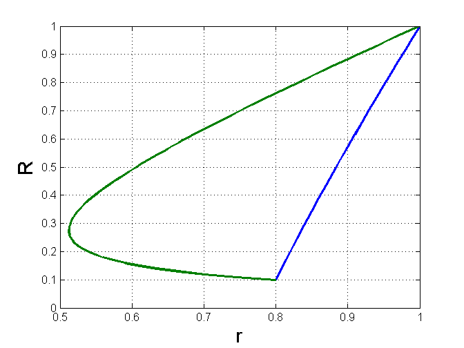
Figure 7: The solid curve shows the transformation defined by (36) for $\{\delta,a,b\}=\{0.1,0.8,1.0\}$. The dashed curve is the mapping (38) for the same cloak parameters.

5.2 Optimal transformation for spherical cloaks

We now take (34) as the definition of the global anisotropy measures. Using again the inverse mapping ${\mbox{\boldmath$\displaystyle\mathbf{X}$}}=f(r)r^{-1}{\mbox{\boldmath$\displaystyle\mathbf{x}$}}$ it follows that $\nabla^{2}{\mbox{\boldmath$\displaystyle\mathbf{X}$}}=[(r^{2}f^{\prime})^{\prime}-2f](fr^{2})^{-1}{\mbox{\boldmath$\displaystyle\mathbf{X}$}}$. The transformation which minimizes $\gamma_{1}$ is therefore

$$f(r)=(b^{3}-a^{3})^{-1}\bigg{[}(b^{3}-a^{2}\delta)r-(a-\delta)b^{3}\frac{a^{2}}{r^{2}}\bigg{]}.$$ (39)

The transformation which minimizes $\gamma_{2}$ is

$$r=(b^{3}-\delta^{3})^{-1}\bigg{[}(b^{3}-a\delta^{2})R+(a-\delta)b^{3}\frac{\delta^{2}}{R^{2}}\bigg{]},$$ (40)

but this again has the unphysical nature found for the 2D case. We conclude that minimization of $\gamma_{2}$ using a single valued function does not appear to have a single or unique solution.

5.3 Numerical examples

The minimizing value of $\gamma_{1}$ may be found by integrating (34a) by parts, and using (35a),

$$\gamma_{1\text{min}}=\begin{cases}\frac{1}{\pi(b^{2}-a^{2})}\left.\big{(}2\pi rff^{\prime}\big{)}\right|_{a}^{b},&\text{2D},\\ \frac{1}{\frac{4}{3}\pi(b^{3}-a^{3})}\left.\big{(}4\pi r^{2}ff^{\prime}\big{)}\right|_{a}^{b},&\text{3D}.\end{cases}$$ (41)

Thus,

$$\gamma_{1\text{min}}=\begin{cases}2\,(b^{2}-a^{2})^{-2}\big{[}(b^{2}-a\delta)^{2}+(a-\delta)^{2}b^{2}\big{]},&\text{2D},\\ 3\,(b^{3}-a^{3})^{-2}\big{[}(b^{3}-a^{2}\delta)^{2}+(a-\delta)^{2}b^{4}\big{]},&\text{3D}.\end{cases}$$ (42)

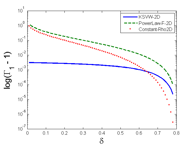
(a) Two dimensions

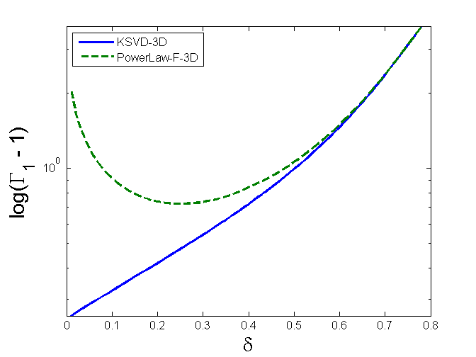
(b) Three dimensions

Figure 8: The relative value of the global anisotropy parameter for the three transformations defined by equation (2) for $\{a,b\}=\{0.8,1.0\}$. The curves show $\log(\Gamma_{1}-1)$ where $\Gamma_{1}=\gamma_{1}/\gamma_{1\text{min}}$, with $\gamma_{1\text{min}}$ given by (42) and $\gamma_{1}$ calculated based on the mappings in equations (2).

The relative value of the anisotropy parameter $\gamma_{1}$ is shown in Figure 8 for the three mappings of equation (2). In all cases, the value of $\gamma_{1}$ exceeds the minimum $\gamma_{1\text{min}}$ for the optimal transformations in equations (36) and (39). The KSVW mapping in 2D has anisotropy only slightly more than the minimum, but for 3D the KSVW displays much larger global anisotropy.

6 Conclusion and discussion

Transformation acoustics, like its close analog transformation optics, possesses a huge freedom in the way that the transformation can be chosen. This paper sheds some light on potential choices. We have shown that is possible to always fix at least one of the three material parameters relevant to radially symmetric deformations. Starting from the theory of Norris Norris (2008), we have derived several forms of the transformation $f$ which yield specialized distributions of material properties such as constant and power law density, radial stiffness, and tangential stiffness. This was achieved by reinterpreting the governing equations for the material properties as differential equations for the transformations. We derived a functional form of $f$ that minimizes elastic anisotropy in a certain sense.

Acknowledgement. We acknowledge funding from the Office of Naval Research (Contract No. N00014-10-C-260) through their SBIR (Small Business Innovative Research Program) under the supervision of Dr. John Tague and Dr. Jan Lindberg.

References

- Norris (2008) A. N. Norris. Acoustic cloaking theory. Proc. R. Soc. A, 464:2411–2434, 2008. 10.1098/rspa.2008.0076.
- Pendry and Li (2008) J. B. Pendry and J. Li. An acoustic metafluid: Realising a broadband acoustic cloak. New J. Phys., 10:115032+, 2008.
- Norris and Shuvalov (2011) A. N. Norris and A. L. Shuvalov. Elastic cloaking theory. Wave Motion, 49:525–538, 2011. 10.1016/j.wavemoti.2011.03.002.
- Zhang et al. (2008) S. Zhang, D. A. Genov, C. Sun, and X. Zhang. Cloaking of matter waves. Phys. Rev. Lett., 100:123002, Mar 2008. 10.1103/PhysRevLett.100.123002.
- Bryan and Leise (2010) K. Bryan and T. Leise. Impedance imaging, inverse problems, and Harry Potter’s Cloak. SIAM Review, 52(2):359–377, 2010. 10.1137/090757873.
- Greenleaf et al. (2009) A. Greenleaf, Y. Kurylev, M. Lassas, and G. Uhlmann. Cloaking devices, electromagnetic wormholes and transformation optics. SIAM Review, 51(1):3–33, 2009.
- Greenleaf et al. (2003) A. Greenleaf, M. Lassas, and G. Uhlmann. Anisotropic conductivities that cannot be detected by EIT. Physiol. Meas., 24(2):413–419, May 2003.
- Chen and Chan (2010) H. Chen and C. T. Chan. Acoustic cloaking and transformation acoustics. J. Phys. D, 43(11):113001+, 2010. 10.1088/0022-3727/43/11/113001.
- Cummer and Schurig (2007) S. A. Cummer and D. Schurig. One path to acoustic cloaking. New J. Phys., 9(3):45+, 2007. 10.1088/1367-2630/9/3/045.
- Chen and Chan (2007) H. Chen and C. T. Chan. Acoustic cloaking in three dimensions using acoustic metamaterials. Appl. Phys. Lett., 91(18):183518+, 2007. 10.1063/1.2803315.
- Cummer et al. (2008) S. A. Cummer, B. I. Popa, D. Schurig, D. R. Smith, J. Pendry, M. Rahm, and A. Starr. Scattering theory derivation of a 3D acoustic cloaking shell. Phys. Rev. Lett., 100(2):024301+, 2008. 10.1103/PhysRevLett.100.024301.
- Pendry et al. (2006) J. B. Pendry, D. Schurig, and D. R. Smith. Controlling electromagnetic fields. Science, 312(5781):1780–1782, 2006. 10.1126/science.1125907.
- Urzhumov et al. (2010) Y. Urzhumov, F. Ghezzo, J. Hunt, and D. R. Smith. Acoustic cloaking transformations from attainable properties. New J. Phys., 12:073014, 2010. 10.1088/1367-2630/12/7/073014.
- Cummer et al. (2009) S. A. Cummer, R. Liu, and T. J. Cui. A rigorous and nonsingular two-dimensional cloaking coordinate transformation. J. Appl. Phys., 105:056102, 2009. 10.1063/1.3080155.
- Kohn et al. (2008) R. V. Kohn, H. Shen, M. S. Vogelius, and M. I. Weinstein. Cloaking via change of variables in electric impedance tomography. Inverse Problems, 24(1):015016+, 2008. 10.1088/0266-5611/24/1/015016.
- (16) Our finite element simulations were carried out with WAI’s commercial finite element code PZFlex®, http://www.pzflex.com, last accessed April 28, 2012.
- Wang et al. (2012) Y-R Wang, H. Zhang, S-Y Zhang, L. Fan, and H-X Sun. Broadband acoustic concentrator with multilayered alternative homogneous materials. JASA Express Letters, 131(2), Feb 2012. 10.1121/1.3679004.
- Rahm et al. (2008) M. Rahm, D. Schurig, D. A. Roberts, S. A. Cummer, D. R. Smith, and J. B. Pendry. Design of electromagnetic cloaks and concentrators using form-invariant coordinate transformations of Maxwell’s equations. In Photonics and Nanostructures - Fundamentals and Applications, volume 6, pages 87–95, 2008. 10.1016/j.photonics.2007.07.013. The Seventh International Symposium on Photonic and Electromagnetic Crystal Structures PECS-VII.
- Li and Pendry (2008) J. Li and J. B. Pendry. Hiding under the carpet: A new strategy for cloaking. Phys. Rev. Lett., 101(20):203901, 2008.