Time periodicity and dynamical stability in two-boson systems

Abstract

We calculate the period of recurrence of dynamical systems comprising two interacting bosons. A number of theoretical issues related to this problem are discussed, in particular, the conditions for small periodicity. The knowledge gathered in this way is then used to propose a notion of dynamical stability based on the stability of the period. Dynamical simulations show good agreement with the proposed scheme. We also apply the results to the phenomenon known as coherent population trapping and find stability conditions in this specific case.

I Introduction

An important result known as the Recurrence Theorem Barreira ; Shepe establishes that quantum as well as classical systems will come very close to their initial state at some time during their evolution. This time is known as the recurrence time, and the theorem applies in the context of closed systems. This kind of recurrence behavior has been observed experimentally in quantum systems such as Rydberg states of the Hydrogen atom Yeazell . A straightforward consequence of the theorem is that closed systems possess, at least in a broad sense, an intrinsic or natural frequency given by the inverse of the recurrence time.

The intrinsic frequency characterizes the response of the system to external driving. The amplitude of the response is maximally enhanced when the driving frequency matches the natural frequency of the system Reslen1 . This enhancement underlies a number of important physical phenomena and its understanding is of fundamental interest. Assuming that the driving frequency is constant, one should minimize fluctuations of the natural frequency in order to amplify the response, especially when the parameters of the system are subject to small perturbations.

Certain classical aspects of stability in two-body systems have been discussed in Politi . Likewise, the stability of quantum dynamics as a result of a small change in the parameters has been discussed in several works, for example in Ref. Prozen or Ref. Peres . In models with classical counterparts, the inner product between quantum states of two systems with the same initial condition but with slightly different parameters remains close to unity during the evolution as long as the initial wave function is well localized inside a stable island of the classical map. The opposite takes place when the initial condition is localized in a chaotic region. Additionally, recurrences in bosonic systems have been studied in Ref. Donovov as a form of state transfer in the time domain. Our proposal is different in that we study Hamiltonians displaying two-body interaction.

Here we intend to approach the issue of stability by studying the behavior of periodicity in a quantum model. The study contains a moderate analysis of the period, which lays the foundation for the subsequent argument concerning stability. In the absence of a classical analogue, we base our approach exclusively on the eigenenergies of the Hamiltonian, making little reference to the initial state.

In this paper we focus initially on a series of issues related to the recurrence period of a two-boson system, particularly, the question of how small the period can be as a function of the parameters. Similarly, we find the set of parameters and the directions along which such parameters must be tuned in order to keep the period constant. Finally, we suggest an application to a quantum optical technique known as coherent population trapping. The results we obtain are also relevant in other scenarios. For instance, in quantum computation, where some information protocols Lisi or quantum gates are subject to perturbations of the parameters. Additionally, this study gives insight into the physics of few-boson systems Cao ; Quiroga ; Blas , which constitute the basis of more complex structures.

In the language of second-quantization, the quantum state is written with reference to occupation modes of unperturbed levels. In this context, let us focus on a model featuring two-body interaction, such as

$$\hat{H}=J(\hat{a}_{1}^{\dagger}\hat{a}_{2}+\hat{a}_{2}^{\dagger}\hat{a}_{1})+\sum_{k=1}^{2}\frac{U_{k}}{2}\hat{a}_{k}^{\dagger}\hat{a}_{k}(\hat{a}_{k}^{\dagger}\hat{a}_{k}-1)+\epsilon_{k}\hat{a}_{k}^{\dagger}\hat{a}_{k}.$$ (1)

As usual, the exchange term $J$ and the unperturbed energies $\epsilon_{1}$ and $\epsilon_{2}$ define the single-body response, while $U_{1}$ and $U_{2}$ determine the intensity of the interaction among particles and can be seen as a nonlinear contribution. The mode operators satisfy the usual bosonic relations $[\hat{a}_{1},\hat{a}_{1}^{\dagger}]=[\hat{a}_{2},\hat{a}_{2}^{\dagger}]=1$, etc. The unperturbed system can be probed by looking at the absorption profile of an incident laser of frequency $\nu=|\epsilon_{2}-\epsilon_{1}|/\hbar$. The total number of particles

$$M=\hat{a}_{1}^{\dagger}\hat{a}_{1}+\hat{a}_{2}^{\dagger}\hat{a}_{2},$$ (2)

is a conserved quantity. The proposed system reduces to a two-level model when $M=1$. Hamiltonian (1) can be rearranged into the form

$$\hat{H}=\eta\hat{a}_{1}^{\dagger}\hat{a}_{1}\hat{a}_{1}^{\dagger}\hat{a}_{1}-\mu\hat{a}_{1}^{\dagger}\hat{a}_{1}+\hat{a}_{1}^{\dagger}\hat{a}_{2}+\hat{a}_{2}^{\dagger}\hat{a}_{1},$$ (3)

where, for $M=2$, the parameters $\eta$, $\mu$ and $\Delta$ turn out to be

$$\eta=\frac{U_{1}+U_{2}}{2J},\text{ }\mu=\frac{3U_{2}+U_{1}}{2J}+\frac{\Delta}{J},\text{ }\Delta=\epsilon_{2}-\epsilon_{1}.$$ (4)

In writing the previous identities we have chosen $J$ to be our energy unit note2 . The state evolution is given by the expression (in what follows, we set $\hbar=1$)

$$|\psi(t)\rangle=q_{1}e^{-iE_{1}t}|E_{1}\rangle+q_{2}e^{-iE_{2}t}|E_{2}\rangle+q_{3}e^{-iE_{3}t}|E_{3}\rangle.$$ (5)

Hence, periodicity arises whenever Godsil

$$E_{1}T=2\pi n_{1},\text{ }E_{2}T=2\pi n_{2},\text{ }E_{3}T=2\pi n_{3}.$$ (6)

where $T$ is the period of the recurrence, and $n_{1}$, $n_{2}$ and $n_{3}$ are integer numbers. In this case the periodicity is absolute as the quantum state recurs identically at regular intervals and the corresponding evolution operator equals the unity operator. Another form of periodicity Ralph emerges by considering instances in which the quantum state recurs up to a phase, i.e.

$$|\psi(t+\tau)\rangle=e^{-i\phi}|\psi(t)\rangle.$$ (7)

We call this partial periodicity, since the phase factor may generate quantum interference effects. As an example, let us look at Hamiltonian (3) for a single particle

$$\hat{H}=\left(\begin{array}[]{cc}-\mu&1\\ 1&0\end{array}\right).$$ (8)

Absolute periodicity occurs whenever the ratio of energies is a fractional number

$$x=\frac{E_{1}}{E_{2}}=\frac{\mu-\sqrt{\mu^{2}+4}}{\mu+\sqrt{\mu^{2}+4}}=\frac{n_{1}}{n_{2}}.$$ (9)

$T$ can be found from Eq. (6)

$$T=2\pi n_{2}\sqrt{-x}=2\pi\sqrt{-n_{1}n_{2}}.$$ (10)

In Eq. (9) we can define $E_{1}$ and $E_{2}$ so that $|n_{2}|\geqslant|n_{1}|$ and therefore $-1\leqslant x<0$. In principle, there is no limit on the maximum value of $T$. Conversely, the minimum value is $T=2\pi$ and takes place at $\mu=0$.

In a similar way, partial periodicity derives from

$$E_{1}\tau=\phi,\text{ }E_{2}\tau=\phi+2\pi,$$ (11)

and therefore

$$\tau=\frac{2\pi}{|E_{2}-E_{1}|}=\frac{2\pi}{\sqrt{\mu^{2}+4}}=2\pi\sqrt{\frac{-x}{(1-x)^{2}}}.$$ (12)

The first equality is consistent with the view that the natural frequency of the system is proportional to the difference of its two eigenenergies. Unlike $T$, $\tau$ reaches a maximum $\tau=\pi$ at $\mu=0$ and goes down asymptotically to zero as $\mu\rightarrow\pm\infty$, two limits in which one of the eigenenergies dominates the spectrum and the Hamiltonian is almost singular. This shows that $\tau$ is maximum when $T$ is minimum and that $\tau$ goes to zero as $T$ goes to infinity. Two-level systems always display partial periodicity, but not necessarily absolute periodicity.

II Two particles

Let us now probe these periodicity concepts in a larger system. For $M=2$, Hamiltonian (3) takes the matrix form

$$\hat{H}=\left(\begin{array}[]{ccc}4\eta-2\mu&\sqrt{2}&0\\ \sqrt{2}&\eta-\mu&\sqrt{2}\\ 0&\sqrt{2}&0\end{array}\right).$$ (13)

The energies are the solutions of the characteristic equation

$$E^{3}+\alpha E^{2}+\beta E+\gamma=0,$$ (14)

where

$$\alpha=-5\eta+3\mu,$$ (15)

$$\beta=2(2\eta-\mu)(\eta-\mu)-4,$$ (16)

$$\mathrm{and}$$ (17)

$$\gamma=4(2\eta-\mu).$$

From the previous equalities we can see that if an energy $E$ is a solution of Eq. (14) for a set of parameters $\{\eta,\mu\}$, then $-E$ is a solution for the set $\{-\eta,-\mu\}$. Additionally, given two solutions $E_{3}$ and $E$ of Eq. (14), it can be shown that

$$E_{3}^{3}-E^{3}+\alpha(E_{3}^{2}-E^{2})+\beta(E_{3}-E)=0.$$ (18)

If $E_{3}\neq E$, the polynomial on the left-hand side can be simplified, and we find that

$$E^{2}+E(E_{3}+\alpha)+E_{3}^{2}+\alpha E_{3}+\beta=0,$$ (19)

so that the respective solutions provide the unaccounted energies

$$\small{E_{1}=-\frac{E_{3}+\alpha+\sqrt{(E_{3}+\alpha)^{2}-4(E_{3}^{2}+\alpha E_{3}+\beta)}}{2},}$$ (20)

and similarly for $E_{2}$. Absolute periodicity results when the energy ratios adhere to the forms

$$x=\frac{E_{1}}{E_{3}}=\frac{n_{1}}{n_{3}},\text{ }y=\frac{E_{2}}{E_{3}}=\frac{n_{2}}{n_{3}}.$$ (21)

One may ask whether, given a set of parameters $\eta$ and $\mu$, the system would display periodicity. This however might not be a convenient approach, since in any case we can find integers $n_{1}$, $n_{2}$ and $n_{3}$ showing ratios as close to $x$ and $y$ as we want. This is also true for any reasonable quantum closed system. Instead, we propose an approach in which, given a pair of ratios, we ask if a set of parameters yielding those ratios exits. Following this idea we proceed as follows.

II.1 Standard Procedure

Let us then consider $x$ and $y$ as known variables. We divide Eq. (20) by $E_{3}$ and find $x$. The variable $y$ is obtained in a similar way. By means of algebraic operations we can express the unknown variables in terms of $\alpha$:

$$E_{3}=-\alpha/(1+x+y),$$ (22)

$$\beta=p\alpha^{2},$$ (23)

$$\gamma=q\alpha^{3},$$ (24)

so that $p$ and $q$ are given by

$$p=(x+y+xy)/(1+x+y)^{2},$$ (25)

$$q=xy/(1+x+y)^{3}.$$ (26)

From Eqs. (15) and (17) we find that

$$\gamma=\frac{4}{3}(\eta-\alpha).$$ (27)

Similarly, using (27) in combination with (24) leads to

$$\eta=\alpha\left(1+\frac{3q}{4}\alpha^{2}\right).$$ (28)

Insertion of Eq. (28) in (15) then yields

$$\mu=2\alpha\left(1+\frac{5q}{8}\alpha^{2}\right).$$ (29)

The combination of Eqs. (16), (23), (28), and (29) leads to the characteristic equation

$$q^{2}A^{3}+2qA^{2}+4pA+16=0,$$ (30)

where $A=\alpha^{2}$. In this way, given a pair of values $x$ and $y$ we find $p$ and $q$ from Eqs. (25) and (26) and introduce them in Eq. (30). From the solutions we find $\alpha$ and therefore the $\eta$ and $\mu$ yielding the energy ratios. Strictly speaking, we have 6 solutions, but they come in pairs giving energies of opposite signs. In order for a solution to be physically acceptable we demand $\eta$ and $\mu$ to be real. Let us next discuss particular cases to which the previous method does not apply.

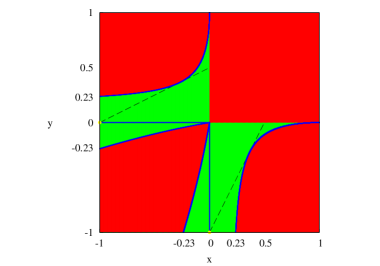
Figure 1: (Color online) Coordinate map indicating the number of set of parameters $\{\eta,\mu\}$ delivering energy ratios $\{x,y\}$. Red (dark gray) region: 0 solutions. Green (light gray) region: 4 solutions. Blue (continuous) lines: 2 solutions. Yellow dots ($\{x=-1,y=0\}$ and $\{x=0,y=-1\}$): 1 solution. Black (dashed) lines highlight the pairs for which there are solutions with $\eta=0$. In these cases, given a couple $\{x,y\}$ there are two solutions with $\eta=0$ and two solutions with $\eta\neq 0$. The mirror symmetry around $y=-x$ derives from the fact that $E_{1}$ and $E_{2}$ can be swapped in Eqs. (21). Here we require $|E_{1}|\leqslant|E_{3}|$ and $|E_{2}|\leqslant|E_{3}|$. Along the edges of the square where $x$ or $y$ is $-1$, there exists an ambiguity in the choice of $E_{3}$ because two eigenenergies display the same absolute value, but their signs are opposite. This implies that the ratio that is different from $-1$ can either be positive or negative. As a consequence, the borders remain identified: $\{x=-1,y\}\sim\{x=-1,-y\}$ and $\{y=-1,x\}\sim\{y=-1,-x\}$.

II.2 Particular Cases

Case A. $\alpha=x+y+1=0$.

For a pair of values $x$ and $y$ the parameter $\eta$ is a solution of the polynomial equation (see appendix A)

$$\kappa^{2}\eta^{6}+27\kappa^{2}\eta^{4}+\left(243\kappa^{2}+\frac{81}{4}\right)\eta^{2}+729\kappa^{2}=0,$$ (31)

where we have introduced

$$\kappa^{2}=-\frac{4}{3+(x-y)^{2}}\left(1-\frac{4}{3+(x-y)^{2}}\right).$$ (32)

Moreover, $\mu$ can be found from Eq. (15).

Case B. $x=1$ or $y=1$ (excluding $\{x=1,y=0\}$, $\{x=0,y=1\}$ and $\{x=y=1\}$).

In order to avoid division by zero in Eq. (18) we modify the variables in the following way

$$\text{if }x=1\Rightarrow x^{\prime}=y^{\prime}=\frac{1}{y},$$ (33)

and analogously when $y=1$. The new variables then admit the standard procedure.

Case C. $\{x=0,y=1\}$ or $\{x=1,y=0\}$.

Then $q=\gamma=0,\beta=-4$ and $\alpha=\eta$. Non-vanishing energy values satisfy $E^{2}+\eta E-4=0$, and $x\text{ (or $y$)}=1$ is a solution only if $\eta=\pm 4i$.

Case D. $\{x=y=1\}$.

The spectrum of the Hamiltonian is threefold degenerate. Hence the eigenvalue equation is of the form $(E_{3}-E)^{3}=0$. Comparing with Eq. (14) we infer that $-3E=\alpha,3E^{2}=\beta$ and $-E^{3}=\gamma$. It then follows that $E^{6}+6E^{4}+12E^{2}+16=0$, which has no real solutions, and therefore no real-valued $\eta$ and $\mu$ yield a fully degenerate spectrum.

Fig. 1 shows a map classifying the coordinate space according to the number of valid solutions encountered for every pair of ratios $\{x,y\}$. The maximum number of solutions is 4, usually coming from 2 real solutions of Eq. (30). Along the negative side of the axes the Hamiltonian becomes reducible with $\mu=2\eta$; hence only two solutions are possible. The two instances with one solution correspond to $\eta=\mu=0$.

II.3 Recurrences

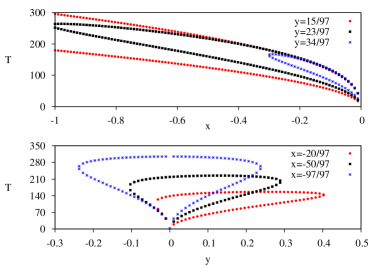
Figure 2: (Color online) Top: Absolute period (arbitrary units) as a function of $x$, with $y$ kept constant. Bottom: Absolute period as a function of $y$, with $x$ kept constant. In both cases the grid slice is $1/97$. As it can be seen, the smallest values of $T$ are found close to the origins.

The condition for absolute periodicity is given in Eq. (5) while partial periodicity can be determined from

$$E_{1}\tau=\phi,\text{ }E_{2}\tau=\phi+2\pi N_{2},\text{ }E_{3}\tau=\phi+2\pi N_{3},$$ (34)

in such a way that $N_{2}$ and $N_{3}$ are both integers. If $T=N\tau$, with $N$ an integer, we can infer from Eqs. (6) and (34) that

$$\phi=\frac{2\pi n_{1}}{N},\text{ }N_{2}=\frac{n_{2}-n_{1}}{N},\text{ }N_{3}=\frac{n_{3}-n_{1}}{N}.$$ (35)

In order to find $T$ and $\tau$, we first determine $n_{1}$, $n_{2}$ and $n_{3}$ from the rationals $x$ and $y$ in such a way that there is no common divisor greater than $1$ among the three generating integers. Simultaneously, $x$ and $y$ are used to find the corresponding eigenenergies following the previously discussed method. We can then choose any of the identities in Eqs. (6) (in particular we choose $E_{3}T=2\pi n_{3}$) to get $T$ using one of the eigenenergies. Finally, the integer $N$ results as the greatest common divider of $n_{2}-n_{1}$ and $n_{3}-n_{1}$. As it can be seen, large integers $n_{3}$ are more likely to yield large $T$ and $\tau$.

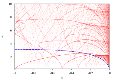
Figure 3: (Color online) Partial period (arbitrary units) as a function of $x$ for $M=2$ and $M=1$ [Eq. (12) - dashed blue line]. We have intentionally restrained the vertical axis to $0<\tau<10$. Interacting Hamiltonians can display longer $\tau$ than non-interacting Hamiltonians. For this particular graph we used grid slices ranging from $1$ to $1/500$ in order to scan the $xy$ square of Fig 1 (see appendix B). Although finer grids would yield denser graphs, these graphs would not be very different from the figure.

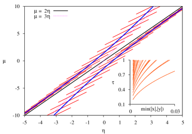
Figure 4: (Color online) Blue lines: set of parameters for which the period is stable under small changes in the direction indicated by the transverse red lines. Inset: $\tau$ (arbitrary units) as a function of the smallest of $|x|$ and $|y|$. It follows that as $\tau$ goes to zero one of the eigenenergies becomes small in comparison to the others.

Figure 2 presents sample plots of $T$ as a function of $x$ and $y$. A complete depiction would be quite more intricate. We point out that $T$ decreases as $x$ and $y$ approach zero. This behavior appears to be generic, laying minimum values of $T$ around (or in) the origins. Following $T$ across the line $\{x=-1/n,y=1/n\}$ for $n=5,6,7,\ldots$, we find that it goes down asymptotically toward $T=\pi\sqrt{2}$ as $n\rightarrow\infty$. The same minimum value can be analytically found at $\{x=-1/2,y=0\}$ and its equivalent. Both instances suggest a relation between the minimum $T$ and the Hamiltonian matrix being or becoming singular.

Fig. 3 depicts the intricate relation between $\tau$ and $x$ obtained by testing energy ratios over the $xy$ square of Fig. 1, as explained in appendix B. Cooperative systems may display longer partial periods than non-interacting systems; therefore, periodicity can help identify interacting phases. This behavior is most likely due to the capacity of many-body systems to develop complex dynamics on account of the increased number of effective states. Also of interest is the chaotic aspect of Fig. 3, indicating that small intervals in $xy$ space do not necessarily map onto small intervals in $\tau$ space. This lack of continuity, which also characterizes $T$, occurs because neighboring values of $x$ and $y$ do not always correspond to neighboring values of $n_{1}$, $n_{2}$ and $n_{3}$. For instance, $\{x=1/3,y=2/3\}$ is not far from $\{x=97/300,y=201/300\}$, but the sets of integers that generate each pair are widely different. Recall that the period depends directly on the integers. In addition, there can be common dividers between $n_{2}-n_{1}$ and $n_{3}-n_{1}$ and this might further affect the continuity of $\tau$. Finally, it can be seen from the inset of Fig. 4 that, when $\tau$ becomes small, at least one of the ratios $x$ or $y$ approaches zero, once again suggesting that in a Hamiltonian displaying small periodicity one of the eigenenergies is much smaller than the others.

III Stability

As introduced here, periodicity, either total or partial, is a characteristic of the Hamiltonian note3 . This encourages us to ask whether one can change the Hamiltonian parameters without affecting the period. This happens for one particle when $\mu=0$, as can be seen from Eq. (12):

$$\left(\frac{d\tau}{d\mu}\right)_{\mu=0}=0.$$ (36)

For two particles, we can start out by arguing that the period is stable whenever both $x$ and $y$ are stable under changes of the parameters. Moreover, we can consider the energy ratios as functions of the parameters, $x(\eta,\mu)$ and $y(\eta,\mu)$, in such a way that maximum variations occur in the direction of the function gradients and zero variations take place in the directions perpendicular to the gradients. In this way, for any set of parameters $\eta$ and $\mu$ one can always identify a direction of change of the parameters along which one of the ratios is stable. It then follows that in order for $T$ to be stable the directions of zero change of both ratios must coincide, i.e., the gradients must be parallel:

$$\vec{\nabla}x+\lambda\vec{\nabla}y=0,$$ (37)

where $\vec{\nabla}x=(\partial x/\partial\eta)\vec{\eta}+(\partial x/\partial\mu)\vec{\mu}$, and similarly for $\vec{\nabla}y$. The vectors $\vec{\eta}$ and $\vec{\mu}$ are unitary vectors in parameter space and $\lambda$ is a real number. This problem is equivalent to finding the extreme values of $x(\eta,\mu)$ subject to the condition $y(\eta,\mu)$=constant, or the other way around. In this context $\lambda$ takes the role of a Lagrange multiplier and the analogy applies as long as the involved functions are smooth. The extremes of $x$ can be worked out from Fig. 1. It is found, however, that not all extreme values imply parallel gradients. For instance, along the edges, where $x$ or $y$ is $-1$, the identification of borders on each side of the axis generates a discontinuity in the first derivative of the ratios and the analogy with the Lagrange method does not apply. Likewise, for the extremes located around the neighborhood of the axes at least one of the parameters diverge toward infinity and there is no solution of Eq. (30) along the positive side of the axes. In general, we find the gradients to be parallel only along the blue (continuous) lines of Fig. 1 located between green and red regions.

Figure 4 shows curves indicating the parameters as well as the directions of change corresponding to zero variation of the period. Far from the origin the curves approach (but do not seem to touch) straight lines given by simple expressions. In one case the direction of zero change aligns with the direction of the curve as we get away from the origin. In the other case the direction of zero change becomes constant with an angle of inclination $\theta$ satisfying $\tan\theta\approx 1/\sqrt{2}$.

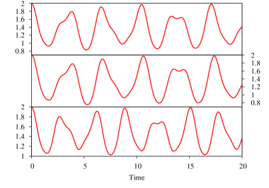
Figure 5: (Color online) Mean number of particles $\langle\hat{a}_{1}^{\dagger}\hat{a}_{1}\rangle$ as a function of time (arbitrary units) for three slightly different cases. Top panel: $\eta=1.878615$ and $\mu=2.939702$. Middle panel: $\eta=1.778615$, $\mu=2.775950$. Bottom panel: $\eta=1.878615$ and $\mu=2.714882$. The middle panel corresponds to a set of parameters in the curve of stability of Fig. 4. The top and bottom plots show the evolution of the system when such parameters are shifted in the direction of zero change and in the direction of the gradient, respectively.

As can be seen from Fig. 5, when the parameters are shifted in the direction of zero change the dynamics of corresponding systems look similar. Conversely, when the change of parameters occurs in the direction of the gradient, the dynamics soon diverge. This behavior is consistent with our study and shows that in certain cases the period alone characterizes the global profile of the system evolution.

III.1 Application to quantum optics: stability condition for coherent population trapping

Besides applicable to systems described by the Hamiltonian (1), our results can be extrapolated to models with analogous Hamiltonians. Let us consider a three-level quantum system interacting with two lasers. We focus on the phenomenon known as coherent population trapping (CPT) Scully . In the semiclassical approach the Hamiltonian can be written in the form

$$\sum_{k=0}^{2}E_{k}|k\rangle\langle k|-\Omega\left(e^{-i\phi_{0}-i\omega_{0}t}|1\rangle\langle 0|+e^{-i\phi_{2}-i\omega_{2}t}|1\rangle\langle 2|+h.c.\right).$$ (38)

Following the notation in Ref. Scully , we define $\Omega e^{-i\phi_{0}}$ and $\Omega e^{-i\phi_{2}}$ as the complex Rabi laser frequencies. We have already assumed that both lasers have the same intensity. $E_{0}$,$E_{1}$, and $E_{2}$ are the eigenenergies of the unperturbed levels, $|0\rangle$, $|1\rangle$ and $|2\rangle$ respectively. We propose a ladder scheme where $E_{2}>E_{1}>E_{0}$. Similarly, $\omega_{0}$ and $\omega_{2}$ are the laser frequencies. CPT means that, as the system evolves, $|1\rangle$ remains unpopulated as a result of quantum interference. The characteristic state of CPT is known as a dark state and is associated to a zero eigenvalue. Measuring energy in units of $\Omega/\sqrt{2}$ Hamiltonian (38) reads

$$\sum_{k=0}^{2}E_{k}^{\prime}|k\rangle\langle k|-\sqrt{2}\left(e^{-i\phi_{0}-i\omega_{0}t}|1\rangle\langle 0|+e^{-i\phi_{2}-i\omega_{2}t}|1\rangle\langle 2|+h.c.\right).$$ (39)

Likewise, introducing the following time-dependent unitary transformation

$$\hat{U}=-e^{-i\phi_{0}-i\omega_{0}t}|0\rangle\langle 0|-e^{-i\phi_{2}-i\omega_{2}t}|2\rangle\langle 2|+|1\rangle\langle 1|,$$ (40)

we find that the transformed state $|\psi_{I}\rangle=\hat{U}|\psi\rangle$ evolves as

$$i\frac{d|\psi_{I}\rangle}{dt}=\left(\hat{H}_{I}+i\left(\frac{d\hat{U}}{dt}\right)\hat{U}^{-1}\right)|\psi_{I}\rangle=\hat{H}_{D}|\psi_{I}\rangle,$$ (41)

so that, $\hat{H}_{I}=\hat{U}\hat{H}\hat{U}^{-1}$ with $\hat{H}$ given by Eq. (39). Evolution is now determined by the time-independent Hamiltonian $\hat{H}_{D}$. Making use of the completeness relation to write $|2\rangle\langle 2|=1-|0\rangle\langle 0|-|1\rangle\langle 1|$, $\hat{H}_{D}$ becomes

$$\left(\begin{array}[]{ccc}\omega_{0}-\omega_{2}-{\Omega}(E_{2}^{\prime}-E_{0}^{\prime})&\sqrt{2}&0\\ \sqrt{2}&-\omega_{2}-(E_{2}^{\prime}-E_{1}^{\prime})&\sqrt{2}\\ 0&\sqrt{2}&0\end{array}\right).$$ (42)

Direct comparison with (13) then establishes that

$$4\eta-2\mu=\omega_{0}-\omega_{2}-\Delta_{0}-\Delta_{2},$$ (43)

$$\eta-\mu=-\omega_{2}-\Delta_{2},$$ (44)

where we have introduced $\Delta_{0}=E_{1}^{\prime}-E_{0}^{\prime}$ and $\Delta_{2}=E_{2}^{\prime}-E_{1}^{\prime}$. In the ratio diagram of Fig. 1, the regions describing a Hamiltonian with one vanishing eigenvalue correspond to the x- and y-axis. These have no intersection with the regions of stability for the total period, which are located between the green and red regions. The partial period is however stable at $\{x=-1,y=0\}$. These ratios correspond to $\eta=\mu=0$. Replacing such values in Eqs. (43) and (44) we find that

$$\omega_{0}=\Delta_{0},$$ (45)

$$\omega_{2}=-\Delta_{2}.$$ (46)

These identities confirm that CPT arises when the frequencies of the lasers coincide with the energy difference between levels. Since CPT is a dynamical phenomenon, it is possible that deviations of the parameters from Eqs. (45) and (46) reduce its efficiency. Nevertheless, since $\tau$ is stable under variations of $\mu$ around $\mu=0$ in the single-particle case, which corresponds to $\eta=0$, we can derive parallel stability conditions for CTP from Eqs. (43) and (44)

$$-2d\mu=d\omega_{0}-d\omega_{2}-d\Delta_{0}-d\Delta_{2},$$ (47)

$$-d\mu=-d\omega_{2}-d\Delta_{2}.$$ (48)

Finally, replacing Eq. (48) in Eq. (47) yields

$$d\Delta_{2}-d\Delta_{0}+d\omega_{2}+d\omega_{0}=0.$$ (49)

It can then be inferred that given a situation where CPT is dominant, i.e., where Eqs. (45) and (46) both hold, the dynamics is stable under small deviations of the parameters as long as such deviations are correlated as in Eq. (49).

IV Conclusions

We studied the time periodicity as well as the stability properties of interacting bosonic systems. The difference between the usual notion of periodicity, in which the ratios of the Hamiltonian energies become commensurate, and partial periodicity, in which the state recurs up to a phase factor, was stressed. Both forms of periodicity were explicitly established for one and two particles in a model described by two bosonic modes. The results suggest a connection between minimum periodicity and the fact that one of the eigenvalues becomes small in comparison to the other eigenvalues, especially in the two-particle case note1 . Similarly, we pointed out that the stability of the period depends not only on the parameters, but also on the direction of change of such parameters. To emphasize this fact, a diagram showing the set of stability parameters as well as the directions of change for which the period stays constant was presented. We found that these results are consistent with simulations of the dynamics and apply the formalism to find stability conditions of CPT.

In should be noted that the assumption $T=N\tau$ made for the two-particle case does not cover the whole set of possilibities of periodicity. It may be possible to relax this assumption and derive $\tau$ using only Eq. (34). This would in principle lead to a richer stability diagram including parameters for which $\tau$ is stable, but $T$ is not, e.g., $\eta=\mu=0$. Similarly, we feel that our method can be extended to more complex Hamiltonians.

Appendix A Appendix A: Derivation of Eq. (31).

When $\alpha=0$ the solutions of Eq. (19) can be written in the form

$$E_{1}=\frac{-E_{3}-\sqrt{-3E_{3}^{2}-4\beta}}{2},\hskip 5.69046ptE_{2}=\frac{-E_{3}+\sqrt{-3E_{3}^{2}-4\beta}}{2}.$$ (50)

It then follows that

$$E_{3}=\sqrt{\frac{-4\beta}{3+(x-y)^{2}}}.$$ (51)

Substituting Eq. (51) in Eq. (14) with $\alpha=0$, we have the equality

$$\kappa\beta^{3/2}=\gamma,$$ (52)

where $\kappa$ is given by Eq. (32). Likewise, from Eq. (15) $\mu=\frac{5}{3}\eta$. Replacing this $\mu$ in Eqs. (16) and (17) gives

$$\beta=-4\left(\frac{\eta^{2}}{9}+1\right),\text{ }\gamma=\frac{4}{3}\eta.$$ (53)

Substitution in Eq. (52) and some algebra then leads to Eq. (31).

Appendix B Appendix B: Generation of commensurate ratios.

In order to generate pairs of ratios compatible with the coordinate square in Fig. 1, we first choose an integer $n_{3}=1,2,3,...$, which is also the inverse of the grid slice. For a given $n_{3}$, we generate integers in the range $-n_{3}<n_{1}<-1$ and $n_{1}<n_{2}<n_{3}-1$. The values of $n_{3}$ are inserted into a computer routine in increasing order, starting with $n_{3}=1$. Subsequently, $n_{1}$ and $n_{2}$ are introduced. These integers determine $x$ and $y$, which are in turn used to check for Hamiltonians with corresponding eigenenergies. Since the coordinate square is symmetric, we only have to scan the section $x<0$. If for the integers in a given triplet $\{n_{1},n_{2},n_{3}\}$ we find a maximum common divider greater than 1, the triplet is discarded. Notice should be taken that in this procedure the coordinate square is scanned using several superimposed grids, avoiding repetition of $\{x,y\}$ pairs.

References

- (1) L. Barreira, XIVth International Congress on Mathematical Physics, 415-422 (2006).
- (2) D.L. Shepelyansky, Phys. Rev. E 82, 055202(R) (2010).
- (3) J. A. Yeazell, M. Mallalieu, and C. R. Stroud, Phys. Rev. Lett. 64 (1990).
- (4) J. Reslen, C.E. Creffield and T.S. Monteiro, Phys. Rev. A 77, 043621 (2008).
- (5) J. De Luca, N. Guglielmi, T. Humphries and A. Politi J. Phys. A: Math. Gen. 43 205103 (2010).
- (6) G. Casati and T. Prosen, Braz. J. Phys. 35, 233 (2005).
- (7) A. Peres, Quantum Theory: Concepts and Methods, ed. by A.V.D Merwe, p 358-368, Kluwer Academic Publishers, (2002).
- (8) M. C. De Oliveira, S. S. Mizrahi, V. V. Dodonov, J. Opt. B: Quant. Semiclas. Opt. 1, 610 (1999).
- (9) P.P. Rohde, A. Fedrizzi and T.C. Ralph, J. Mod. Opt. 59, 710 (2012).
- (10) S.M. Giampaolo, F. Illuminati and A. Di Lisi, G. Mazzarella, Int. J. Quant. Inf. 4, 507 (2006).
- (11) C. Godsil, Elec. J. Comb., 18 23 (2011).
- (12) Cao L, Brouzos I, Zöllner S and Schmelcher, New J. Phys., 13 033032 (2011).
- (13) L.J. Salazar, D. A. Guzmán, F.J. Rodríguez and L. Quiroga, Optics Express, 20, p. 4470-4483 (2012).
- (14) B. M. Rodríguez-Lara, A. Zárate-Cárdenas, F. Soto-Eguibar and H.M. Moya-Cessa, arXiv:1207.6552.
- (15) As usually depends on the details of the system, we avoid making reference to it and use arbitrary units for our time scales.
- (16) This statement is valid as long as the initial state is not an eigenstate of the Hamiltonian.
- (17) The only exception takes place for one particle when since according to Eqs. (9) and (10) .
- (18) M.O. Scully and M.S. Zubairy, Quantum Optics, Cambridge University Press, p 223-225, (1997).