A Benes Packet Network

Longbo Huang, Jean Walrand Longbo Huang (http://www.eecs.berkeley.edu/similar-to\simhuang) and Jean Walrand (http://www.eecs.berkeley.edu/similar-to\simwlr) are with the EECS department of University of California, Berkeley, CA, 94720.
Abstract

Benes networks are constructed with simple switch modules and have many advantages, including small latency and requiring only an almost linear number of switch modules. As circuit-switches, Benes networks are rearrangeably non-blocking, which implies that they are full-throughput as packet switches, with suitable routing.

Routing in Benes networks can be done by time-sharing permutations. However, this approach requires centralized control of the switch modules and statistical knowledge of the traffic arrivals. We propose a backpressure-based routing scheme for Benes networks, combined with end-to-end congestion control. This approach achieves the maximal utility of the network and requires only four queues per module, independently of the size of the network.

Index Terms:
Benes Network, Dynamic Control, Stochastic Network Optimization, Queueing

I Introduction

Data centers have gradually become one of our most important computing resources. For instance, search engines, web emails such as Gmail and Hotmail, social network websites such as Facebook, and data processing applications such as Hadoop are provided by data centers. Consequently, the networking of servers and resource allocation in data centers have become important problems.

We develop a networking solution, a Benes packet network, which consists of a Benes architecture, a flow utility maximization mechanism, and a backpressure-based scheduling algorithm. Specifically, we propose interconnecting the data center servers using a Benes network built with simple commodity switch modules. We formulate the resource allocation objective as a network flow utility maximization problem to guarantee a fair share of the network resources. Lastly, we develop a low-complexity backpressure-based scheduling algorithm, called Grouped-Backpressure (G-BP), to achieve the optimal system performance. The G-BP algorithm is provably optimal and automatically handles changing traffic. Our approach only requires each switch module to maintain four queues, independently of the network size, and hence can easily be implemented in practice.

Many papers explore networking solutions for data centers. [1] proposes using a random graph based approach to enable incremental network growth for data centers. [2] proposes a network architecture based on Clos network and random traffic splitting. [3] develops a hierarchical network structure for data centers. [4] uses the preferential attachment approach to design network topologies for data centers. [5] proposes a fat-tree based network architecture. [6] develops a MapReduce-like system based on a cube-like architecture to exploit the in-network aggregation possibilities. [7] designs optical networks for data centers. However, we note that the aforementioned works mostly focus on designing the network architecture and achieving uniform load balancing. Hence, the proposed solutions do not immediately apply to problems where different flows have different service requirements. Moreover, the solutions developed in the above works lack system performance guarantees.

In this work, we aim at obtaining a network solution that combines practicality, generality, provable optimality, and low complexity. Specifically, we propose interconnecting the data center servers by a Benes network. As circuit-switches, Benes networks are known to be rearrangeably non-blocking and can easily be built with only an almost linear number of simple switch modules in the network size [8], [9]. Thus, adopting the Benes network architecture not only guarantees high system throughput and low end-to-end packet delay (if routing and scheduling are done properly), but also eliminates the need for employing expensive switch devices whose cost does not scale easily as the data center size increases. Under the Benes network architecture, we establish a mathematical formulation for determining the allocation of network resources to cope with the heterogeneity of the data traffic service requirements. Our formulation leverages the network utility maximization framework [10], [11], which has been proven to be a general mechanism for handling network resource allocation problems.

Finally, to reap the full benefits of the Benes network architecture and the resource allocation framework in a practical manner, we develop a routing and scheduling algorithm that has provable system performance guarantees and a very low implementation complexity. Our algorithm is constructed based on the recently developed backpressure network optimization technique [12], combined with an end-to-end congestion control mechanism. However, different from previous backpressure algorithms, e.g., [13], [14], [15], which either require that the number of queues each switch module has to maintain is proportional to the network size, or only apply to problems with single-path routing, our algorithm uses a novel traffic grouping idea and allows us to use only four queues per switch module regardless of the network size. Moreover, our algorithm automatically explores all the possible routes to fully utilize network capacity. These distinct features make our algorithm very suitable for practical implementation.

This paper is organized as follows. In Section II, we present the system model and state our objective. In Section III, we set up the notations. Then, we explain the intuition of our design approach and describe all the needed components of the Group-Backpressure (G-BP) algorithm in Section IV. We present the G-BP algorithm and analyze its performance in Section V. Simulation results are presented in Section VI. We conclude the paper in Section VII.

II System model

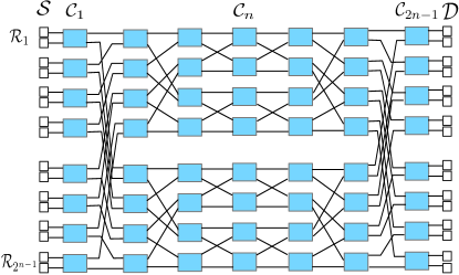
We consider the system shown in Fig. 1, where a Benes network connects a set of communicating servers. In this system, each rectangle is a switch module having two input and two output links. Each link has a capacity of 111 packet/slot. The smaller nodes are the servers. Traffic flows are generated from the servers on the left, called input servers, and are going to the servers on the right, called output servers. 111It is straightforward to extend our results to include bi-directional traffic flows. We assume that the system operates in slotted time, i.e., t{0,1,2,}𝑡012t\in\{0,1,2,...\}. The discrete time assumption is for convenience of the analysis. The actual network would operate in an asynchronous way with variable length packets.
Refer to caption
Figure 1: A 16×16161616\times 16 Benes network connecting 161616 input servers 𝒮𝒮{\cal S} to 161616 output servers 𝒟𝒟{\cal D}. The rectangles are the switch modules that form the Benes network. isubscript𝑖{{\cal{R}}}_{i} refers to row i𝑖i of the Benes network and 𝒞jsubscript𝒞𝑗{{\cal{C}}}_{j} refers to column j𝑗j.

II-A Admission control and flow utility

We label the flows according to their source and destination servers. Specifically, we call the traffic entering from input server s𝑠s and going to output server d𝑑d the (s,d)𝑠𝑑(s,d) flow. We use Asd(t)subscript𝐴𝑠𝑑𝑡A_{sd}(t) to denote the number of (s,d)𝑠𝑑(s,d) packets generated at input server s𝑠s at time t𝑡t. We assume that for every (s,d)𝑠𝑑(s,d) flow, the random variables {Asd(t),t=0,1,}formulae-sequencesubscript𝐴𝑠𝑑𝑡𝑡01\{A_{sd}(t),t=0,1,\ldots\} are i.i.d. and have mean λsd=𝔼[Asd(t)]subscript𝜆𝑠𝑑𝔼delimited-[]subscript𝐴𝑠𝑑𝑡\lambda_{sd}=\mathbb{E}\big{[}A_{sd}(t)\big{]}. Our results can be extended to incorporate much more general arrival processes, e.g., Makov-modulated arrivals. We also assume that there exists some finite constant Amaxsubscript𝐴A_{\max} such that 0Asd(t)Amax0subscript𝐴𝑠𝑑𝑡subscript𝐴0\leq A_{sd}(t)\leq A_{\max} for all (s,d)𝑠𝑑(s,d) and for all time t𝑡t.

In every time slot t𝑡t, each input server performs admission control to determine how many packets to inject into the network. We denote 0Rsd(t)Asd(t)0subscript𝑅𝑠𝑑𝑡subscript𝐴𝑠𝑑𝑡0\leq R_{sd}(t)\leq A_{sd}(t) the number of (s,d)𝑠𝑑(s,d) flow packets actually admitted by input server s𝑠s for transmission at time t𝑡t. We then denote the average rate of the (s,d)𝑠𝑑(s,d) flow packets by rsdsubscript𝑟𝑠𝑑r_{sd}, defined as: 222Throughout this paper, we assume that all the limits exist.

rsdlimT1Tt=0T1𝔼[Rsd(t)].subscript𝑟𝑠𝑑subscript𝑇1𝑇superscriptsubscript𝑡0𝑇1𝔼delimited-[]subscript𝑅𝑠𝑑𝑡\displaystyle r_{sd}\triangleq\lim_{T\rightarrow\infty}\frac{1}{T}\sum_{t=0}^{T-1}\mathbb{E}\big{[}R_{sd}(t)\big{]}. (1)

Each (s,d)𝑠𝑑(s,d) flow is associated with a utility function Usd(rsd)subscript𝑈𝑠𝑑subscript𝑟𝑠𝑑U_{sd}(r_{sd}), which is concave increasing in its average rate rsdsubscript𝑟𝑠𝑑r_{sd}. We assume that the utility functions have finite first derivatives and denote β𝛽\beta their maximum value, i.e.,

βmaxsdUsd(0).𝛽subscript𝑠𝑑subscriptsuperscript𝑈𝑠𝑑0\displaystyle\beta\triangleq\max_{sd}U^{\prime}_{sd}(0). (2)

II-B Stability and objective

In this paper, we say that a queue with queue size process {Q(t)0,t=0,1,2,}formulae-sequence𝑄𝑡0𝑡012\{Q(t)\geq 0,t=0,1,2,...\} is stable if:

lim supT1Tt=0T1𝔼[Q(t)]<.subscriptlimit-supremum𝑇1𝑇superscriptsubscript𝑡0𝑇1𝔼delimited-[]𝑄𝑡\displaystyle\limsup_{T\rightarrow\infty}\frac{1}{T}\sum_{t=0}^{T-1}\mathbb{E}\big{[}Q(t)\big{]}<\infty. (3)

Then, we say that a network is stable if all the queues in the network are stable, and call a routing and scheduling policy that ensures network stability a stabilizing policy. We use ΛnsubscriptΛ𝑛\Lambda_{n} to denote the capacity region of a 2n×2nsuperscript2𝑛superscript2𝑛2^{n}\times 2^{n} Benes network, being the set of arrival vectors under which there exist stabilizing routing and scheduling policies.

Depending on the routing and scheduling algorithm, the network queueing structure can be quite different. Our objective is to find a low-implementation-complexity stabilizing routing and scheduling policy that maximizes the aggregate flow utility of the network, i.e.,

max::absent\displaystyle\max: U(𝒓)s,dUsd(rsd)𝑈𝒓subscript𝑠𝑑subscript𝑈𝑠𝑑subscript𝑟𝑠𝑑\displaystyle U({\boldsymbol{r}})\triangleq\sum_{s,d}U_{sd}(r_{sd}) (4)
s.t. 𝒓Λn,𝒓subscriptΛ𝑛\displaystyle{\boldsymbol{r}}\in\Lambda_{n},

where 𝒓=(rsd,(s,d))𝒓subscript𝑟𝑠𝑑for-all𝑠𝑑{\boldsymbol{r}}=(r_{sd},\,\forall\,(s,d)) with rsdsubscript𝑟𝑠𝑑r_{sd} being the average rate of the (s,d)𝑠𝑑(s,d) flow defined in (1). We denote by 𝒓optsuperscript𝒓opt{\boldsymbol{r}}^{\textsf{opt}} the rate vector that achieves the optimal utility over all stabilizing policies.

Note that our formulation (4) is indeed very general. The heterogeneity of traffic flow service requirements can easily be taken into account by designing appropriate utility functions. Also note that, although our system model is similar to those in [13], in our paper, the queueing structure is also part of the algorithm design problem.

II-C Discussion

The problem of optimal routing and scheduling in a Benes network can be solved by using the well-known backpressure routing algorithm [12]. However, this approach requires each node to maintain a separate queue for each output server. Thus, each node has to maintain 2nsuperscript2𝑛2^{n} queues, which is not practical when the size of the Benes network (number of servers) increases. Recent works [14] and [15] propose backpressure-based algorithms that use much fewer queues. However, the algorithm in [14] requires nodes to maintain a separate queue for each cluster of the network nodes and needs a pre-defined clustering algorithm, whereas the method in [15] is designed for single-path routing. Below, we develop a novel low-complexity approach called Grouped-Backpressure (G-BP). Our approach allows us to use only four queues per node regardless of the network size.

III Benes network structure and labeling

In this section, we explain the structure of Benes networks and set up our notations.

III-A Benes network construction

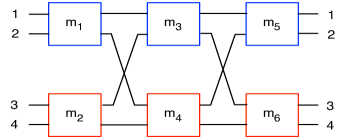
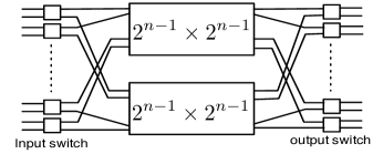
We first explain how a 2n×2nsuperscript2𝑛superscript2𝑛2^{n}\times 2^{n} Benes network is constructed [8] [9]: Start with a basic 2×2222\times 2 Benes network as in Fig. 2(a). Then, construct a 2n×2nsuperscript2𝑛superscript2𝑛2^{n}\times 2^{n} Benes network as follows:

(Step I)-Concatenation: Vertically concatenate two 2n1×2n1superscript2𝑛1superscript2𝑛12^{n-1}\times 2^{n-1} Benes networks. Call them the upper subnetwork and the lower subnetwork, e.g., m3subscript𝑚3m_{3} and m4subscript𝑚4m_{4} in Fig. 2(b). Then, horizontally place two columns of 2n1superscript2𝑛12^{n-1} basic 2×2222\times 2 modules, one on each side of the concatenated subnetworks. Call the modules on the left of the concatenated subnetworks the input switch modules, e.g., m1subscript𝑚1m_{1} and m2subscript𝑚2m_{2}, and the modules on the right the output switch modules, e.g., m5subscript𝑚5m_{5} and m6subscript𝑚6m_{6}.

(Step II)-Connect input modules: Connect the upper output link of the input module in row k𝑘k to the kthsuperscript𝑘thk^{\text{th}} input link of the upper subnetwork, and connect its lower output link to the kthsuperscript𝑘thk^{\text{th}} input link of the lower subnetwork.

(Step III)-Connect output modules: Connect the kthsuperscript𝑘thk^{\text{th}} output link of the upper subnetwork to the upper input link of the kthsuperscript𝑘thk^{\text{th}} output module, i.e., the output module in row k𝑘k, and connect the kthsuperscript𝑘thk^{\text{th}} output link of the lower subnetwork to the lower input link of the kthsuperscript𝑘thk^{\text{th}} output module.

Refer to caption
(a) A basic 2×2222\times 2 Benes network
Refer to caption
(b) A 4×4444\times 4 Benes network
Refer to caption
(c) A general 2n×2nsuperscript2𝑛superscript2𝑛2^{n}\times 2^{n} Benes network
Figure 2: The structure of Benes networks.

III-B Labeling a Benes network with servers

We first specify how we label a 2n×2nsuperscript2𝑛superscript2𝑛2^{n}\times 2^{n} Benes network. We denote 𝔹nsubscript𝔹𝑛\mathbb{B}_{n} the 2n×2nsuperscript2𝑛superscript2𝑛2^{n}\times 2^{n} Benes network (excluding the input and output servers). Then, we divide the Benes network into rows and columns. In a 2n×2nsuperscript2𝑛superscript2𝑛2^{n}\times 2^{n} Benes network, there are 2n1superscript2𝑛12^{n-1} rows, denoted by {i,i=1,,2n1}formulae-sequencesubscript𝑖𝑖1superscript2𝑛1\{{{\cal{R}}}_{i},i=1,...,2^{n-1}\}. We then denote the 2n12𝑛12n-1 columns by {𝒞j,j=1,,2n1}formulae-sequencesubscript𝒞𝑗𝑗12𝑛1\{{{\cal{C}}}_{j},j=1,...,2n-1\}. For any node m𝑚m in the Benes network, we use imsubscript𝑖𝑚i_{m} and jmsubscript𝑗𝑚j_{m} to denote its row number and column number. For the input and output servers connecting to the Benes network, we label them using their row numbers. The set of input servers are denoted by 𝒮={1,2,,2n}𝒮12superscript2𝑛{{\cal{S}}}=\{1,2,...,2^{n}\} and the set of output servers are denoted by 𝒟={1,2,,2n}𝒟12superscript2𝑛{{\cal{D}}}=\{1,2,...,2^{n}\}. Note that both 𝒮𝒮{{\cal{S}}} and 𝒟𝒟{{\cal{D}}} have 2nsuperscript2𝑛2^{n} rows (the small squares in Fig. 1). As in Section III-A, we call the nodes in 𝒞1subscript𝒞1{{\cal{C}}}_{1} the input switch modules and the nodes in 𝒞2n1subscript𝒞2𝑛1{{\cal{C}}}_{2n-1} the output switch modules.

From the construction rules of Benes networks and the way the servers are connected to the Benes network, we see that for every node m𝔹n𝑚subscript𝔹𝑛m\in\mathbb{B}_{n}, there are two nodes in column 𝒞jm+1subscript𝒞subscript𝑗𝑚1{{\cal{C}}}_{j_{m}+1} to which it connects (for a node m𝒞2n1𝑚subscript𝒞2𝑛1m\in{{\cal{C}}}_{2n-1}, it connects to two nodes in 𝒟𝒟{{\cal{D}}}). We denote the node with a smaller row number by musubscript𝑚𝑢m_{u} and the other one by mlsubscript𝑚𝑙m_{l}. There are also two nodes in column 𝒞jm1subscript𝒞subscript𝑗𝑚1{{\cal{C}}}_{j_{m}-1} that connect to m𝑚m (if m𝒞1𝑚subscript𝒞1m\in{{\cal{C}}}_{1}, there are two nodes in 𝒮𝒮{{\cal{S}}} connecting to it). We denote these two nodes by msubscript𝑚{{\cal{M}}}_{m}. Among these nodes, those that have m𝑚m as their next hop with a smaller row number are denoted by musuperscriptsubscript𝑚𝑢{{\cal{M}}}_{m}^{u}, and the other nodes having m𝑚m as their next hop node with a larger row number are denoted by mlsuperscriptsubscript𝑚𝑙{{\cal{M}}}_{m}^{l}, i.e.,

mu={m𝒞jm1|mu=m},superscriptsubscript𝑚𝑢conditional-setsuperscript𝑚subscript𝒞subscript𝑗𝑚1subscriptsuperscript𝑚𝑢𝑚\displaystyle{{\cal{M}}}_{m}^{u}=\{m^{\prime}\in{{\cal{C}}}_{j_{m}-1}\,\,|\,\,m^{\prime}_{u}=m\},
ml={m𝒞jm1|ml=m}.superscriptsubscript𝑚𝑙conditional-setsuperscript𝑚subscript𝒞subscript𝑗𝑚1subscriptsuperscript𝑚𝑙𝑚\displaystyle{{\cal{M}}}_{m}^{l}=\{m^{\prime}\in{{\cal{C}}}_{j_{m}-1}\,\,|\,\,m^{\prime}_{l}=m\}.

For m𝒞1𝑚subscript𝒞1m\in{{\cal{C}}}_{1}, we simply use msubscript𝑚{{\cal{M}}}_{m} to denote the input servers that connect to it. For each input server s𝒮𝑠𝒮s\in{{\cal{S}}}, we use m(s)𝑚𝑠m(s) to denote the node in 𝒞1subscript𝒞1{{\cal{C}}}_{1} it connects to. We call the servers in rows 111 to 2n1superscript2𝑛12^{n-1} the upper division servers, and call all the other servers the lower division servers. We then call a flow whose destination is an upper division server an upper division flow. Otherwise it is a lower division flow.

For a 2n×2nsuperscript2𝑛superscript2𝑛2^{n}\times 2^{n} Benes network 𝔹nsubscript𝔹𝑛\mathbb{B}_{n}, we define the nodes in 𝒞nsubscript𝒞𝑛{{\cal{C}}}_{n} as the partition nodes. From the construction rules of the Benes networks, we first have the following observation:

Fact 1

For a 2n×2nsuperscript2𝑛superscript2𝑛2^{n}\times 2^{n} Benes network, its partition nodes coincide with the partition nodes of its two 2n1×2n1superscript2𝑛1superscript2𝑛12^{n-1}\times 2^{n-1} subnetworks. \Diamond

Below, we denote the upper outgoing link of a switch module by link a𝑎a and the lower outgoing link by link b𝑏b (see Fig. 2(a)). We use 𝒪masuperscriptsubscript𝒪𝑚𝑎{{\cal{O}}}_{m}^{a} to denote the set of output servers that can be reached by traversing the upper outgoing link a𝑎a of node m𝑚m and use 𝒪mbsuperscriptsubscript𝒪𝑚𝑏{{\cal{O}}}_{m}^{b} to denote the set of output servers that can be reached by traversing link b𝑏b. We then have the following simple lemma, which can be seen from the construction rules of Benes networks.

Lemma 1

(a) Starting from any partition node m𝒞n𝑚subscript𝒞𝑛m\in{{\cal{C}}}_{n}, there is a unique path to any output server d𝒟𝑑𝒟d\in{{\cal{D}}}. (b) For every node m𝒞n+l,l0formulae-sequence𝑚subscript𝒞𝑛𝑙𝑙0m\in{{\cal{C}}}_{n+l},l\geq 0, we have:

𝒪ma={κm2nl+1,,(κm+12)2nl},superscriptsubscript𝒪𝑚𝑎subscript𝜅𝑚superscript2𝑛𝑙1subscript𝜅𝑚12superscript2𝑛𝑙\displaystyle{{\cal{O}}}_{m}^{a}=\{\kappa_{m}2^{n-l}+1,...,(\kappa_{m}+\frac{1}{2})2^{n-l}\}, (5)
𝒪mb={(κm+12)2nl+1,,(κm+1)2nl},superscriptsubscript𝒪𝑚𝑏subscript𝜅𝑚12superscript2𝑛𝑙1subscript𝜅𝑚1superscript2𝑛𝑙\displaystyle{{\cal{O}}}_{m}^{b}=\{(\kappa_{m}+\frac{1}{2})2^{n-l}+1,...,(\kappa_{m}+1)2^{n-l}\}, (6)

where κm(im1)mod2lsubscript𝜅𝑚modulosubscript𝑖𝑚1superscript2𝑙\kappa_{m}\triangleq(i_{m}-1)\mod 2^{l}. \Diamond

IV Intuition and key components of Grouped-Backpressure

In this section, we present the idea and all the needed components for our Grouped-Backpressure algorithm (G-BP), which will be used to achieve the optimal flow utility under the Benes network architecture.

IV-A The idea

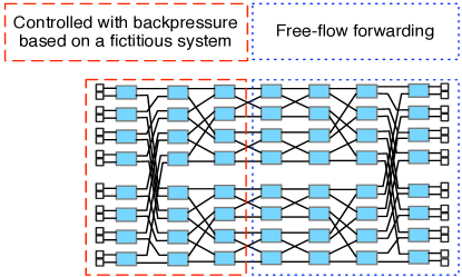
The idea of Grouped-Backpressure is to “group” all the flows into two mixed flows, the upper division flow and the lower division flow. Then, we construct a scheme for routing the mixed traffic in the first half of the network based on a fictitious reference system. This approach allows us to use very few queues per node. However, due to this traffic mixing, we lose the ability to control each individual flow inside the network. Hence, the flows can be routed arbitrarily inside the network, in which case certain nodes may receive more traffic than they can handle and become unstable. In order to resolve this problem, we impose a special queueing structure at each node to ensure that routing and scheduling is done in a fully symmetric manner. With this approach, we guarantee that every flow is split into sub-flows with equal rates and routed through the partition nodes. In the second half of the network, by Lemma 1, each packet will traverse a unique path to its destination. Hence, we will do a “free-flow” routing. Using the symmetric structure of the Benes network, we then show that the G-BP algorithm can stabilize the network and achieve maximum utility. Our approach is demonstrated in Fig. 3.
Refer to caption
Figure 3: The pictorial illustration of the G-BP algorithm. The first half of the network is controlled by a backpressure-like algorithm based on a fictitious reference system. The second half of the network uses a “free-flow” scheme for packet delivery.

IV-B A fictitious reference system

In order to guide the routing and scheduling of the grouped traffic, we create a fictitious reference system as follows.

  1. 1.

    Remove all the nodes in columns n+1𝑛1n+1 to 2n12𝑛12n-1.

  2. 2.

    Create two fictitious destination nodes D1subscript𝐷1D_{1} and D2subscript𝐷2D_{2}, where D1subscript𝐷1D_{1} represents the common destination for the upper division flows and D2subscript𝐷2D_{2} represents the common destination for the lower division flows.

  3. 3.

    Connect each partition node, i.e., a node in 𝒞nsubscript𝒞𝑛{{\cal{C}}}_{n}, to D1subscript𝐷1D_{1} with a link of capacity 111 packet/slot and to D2subscript𝐷2D_{2} with a link of capacity 111 packet/slot.

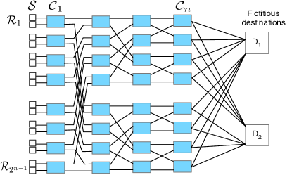
An example of the fictitious system is shown in Fig. 4 for a 16×16161616\times 16 Benes network. The fictitious system will be used as a reference system to guide us on serving the grouped traffic. Specifically, we will design a backpressure-based algorithm for the fictitious system, and use the exact same actions to control the nodes in columns 111 to n1𝑛1n-1 in the physical system. This approach has the useful property that it allows us to use only 444 queues per node.

Refer to caption
Figure 4: The fictitious reference system for the 16×16161616\times 16 Benes network with servers.

IV-C Queue structure and load balancing

Since in the reference system we only have 222 destinations and do not distinguish flows inside the network, if routing is not done carefully, it can happen that most of the traffic going to an output port is routed to a single partition node and causes instability of the node. In order to resolve this issue, we impose a special queueing structure on the switch nodes to balance all the traffic, so that each flow is equally split among all possible paths and routed to the partition nodes. Doing so, we guarantee that as long as the traffic rate is supportable (will be explained later), no node will be overwhelmed.

We now specify our queueing structure for both the fictitious system and the physical system:

IV-C1 Input servers in both systems

For each input server s𝒮𝑠𝒮s\in{{\cal{S}}}, we maintain 222 queues per node as follows:

  • QsU(t)superscriptsubscript𝑄𝑠U𝑡Q_{s}^{\textsf{U}}(t): number of upper division flow packets stored at input server s𝑠s;

  • QsL(t)superscriptsubscript𝑄𝑠L𝑡Q_{s}^{\textsf{L}}(t): number of lower division flow packets stored at input server s𝑠s.

These two queues evolve according to the following dynamics:

Qs𝒯(t+1)=[Qs𝒯(t)μs,m(s)𝒯(t)]++Rs𝒯(t).superscriptsubscript𝑄𝑠𝒯𝑡1superscriptdelimited-[]superscriptsubscript𝑄𝑠𝒯𝑡superscriptsubscript𝜇𝑠𝑚𝑠𝒯𝑡superscriptsubscript𝑅𝑠𝒯𝑡\displaystyle Q_{s}^{{{\cal{T}}}}(t+1)=\big{[}Q_{s}^{{{\cal{T}}}}(t)-\mu_{s,m(s)}^{{{\cal{T}}}}(t)\big{]}^{+}+R_{s}^{{{\cal{T}}}}(t). (7)

Here the notation [x]+=max[x,0]superscriptdelimited-[]𝑥𝑥0[x]^{+}=\max[x,0] and the notation 𝒯Ωs{U,L}𝒯subscriptΩ𝑠UL{{\cal{T}}}\in\Omega_{s}\triangleq\{{{\cal{\textsf{U},\textsf{L}}}}\} denotes the “type” of the traffic at the input servers, and Rs𝒯(t)superscriptsubscript𝑅𝑠𝒯𝑡R_{s}^{{{\cal{T}}}}(t) denotes the aggregate arrival to Qs𝒯(t)superscriptsubscript𝑄𝑠𝒯𝑡Q_{s}^{{{\cal{T}}}}(t), i.e.,

RsU(t)=d2n1Rsd(t),RsL(t)=d>2n1Rsd(t).formulae-sequencesuperscriptsubscript𝑅𝑠U𝑡subscript𝑑superscript2𝑛1subscript𝑅𝑠𝑑𝑡superscriptsubscript𝑅𝑠L𝑡subscript𝑑superscript2𝑛1subscript𝑅𝑠𝑑𝑡\displaystyle R_{s}^{\textsf{U}}(t)=\sum_{d\leq 2^{n-1}}R_{sd}(t),\,\,R_{s}^{\textsf{L}}(t)=\sum_{d>2^{n-1}}R_{sd}(t). (8)

IV-C2 Switch modules in columns 111 to n1𝑛1n-1 in both systems

We maintain 444 queues per node as follows:

  • QmUU(t)superscriptsubscript𝑄𝑚UU𝑡Q_{m}^{\textsf{UU}}(t): number of upper division flow packets that will be routed through musubscript𝑚𝑢m_{u};

  • QmUL(t)superscriptsubscript𝑄𝑚UL𝑡Q_{m}^{\textsf{UL}}(t): number of upper division flow packets that will be routed through mlsubscript𝑚𝑙m_{l};

  • QmLU(t)superscriptsubscript𝑄𝑚LU𝑡Q_{m}^{\textsf{LU}}(t): number of lower division flow packets that will be routed through musubscript𝑚𝑢m_{u};

  • QmLL(t)superscriptsubscript𝑄𝑚LL𝑡Q_{m}^{\textsf{LL}}(t): number of lower division flow packets that will be routed through mlsubscript𝑚𝑙m_{l}.

Now define ΩB{UU,UL,LU,LL}subscriptΩ𝐵UUULLULL\Omega_{B}\triangleq\{\textsf{UU},\textsf{UL},\textsf{LU},\textsf{LL}\} and use 𝒯ΩB𝒯subscriptΩ𝐵{{\cal{T}}}\in\Omega_{B} to denote the type of these queues at the switch nodes. We see that the queues evolve according to the following dynamics:

Qm𝒯(t+1)superscriptsubscript𝑄𝑚𝒯𝑡1\displaystyle Q_{m}^{{{\cal{T}}}}(t+1) (9)
[Qm𝒯(t)μm,m(𝒯)𝒯(t)]++Rm𝒯(t),𝒯ΩB.formulae-sequenceabsentsuperscriptdelimited-[]superscriptsubscript𝑄𝑚𝒯𝑡superscriptsubscript𝜇𝑚𝑚𝒯𝒯𝑡superscriptsubscript𝑅𝑚𝒯𝑡for-all𝒯subscriptΩ𝐵\displaystyle\qquad\quad\leq\big{[}Q_{m}^{{{\cal{T}}}}(t)-\mu_{m,m({{\cal{T}}})}^{{{\cal{T}}}}(t)\big{]}^{+}+R_{m}^{{{\cal{T}}}}(t),\,\forall\,{{\cal{T}}}\in\Omega_{B}.

Here m(𝒯)𝑚𝒯m({{\cal{T}}}) is the next hop node corresponding to the type 𝒯𝒯{{\cal{T}}} traffic, i.e., m(𝒯)=mu𝑚𝒯subscript𝑚𝑢m({{\cal{T}}})=m_{u} for 𝒯{UU,LU }𝒯UULU {{\cal{T}}}\in\{\textsf{UU},\textsf{LU }\} and m(𝒯)=ml𝑚𝒯subscript𝑚𝑙m({{\cal{T}}})=m_{l} otherwise. Rm𝒯(t)superscriptsubscript𝑅𝑚𝒯𝑡R_{m}^{{{\cal{T}}}}(t) is the aggregate arrivals to Qm𝒯(t)superscriptsubscript𝑄𝑚𝒯𝑡Q_{m}^{{{\cal{T}}}}(t), given by:

RmUU(t)=Xm(t)RmU(t),RmUL(t)=(1Xm(t))RmU(t),formulae-sequencesuperscriptsubscript𝑅𝑚UU𝑡subscript𝑋𝑚𝑡superscriptsubscript𝑅𝑚U𝑡superscriptsubscript𝑅𝑚UL𝑡1subscript𝑋𝑚𝑡superscriptsubscript𝑅𝑚U𝑡\displaystyle R_{m}^{\textsf{UU}}(t)=X_{m}(t)R_{m}^{\textsf{U}}(t),\,\,R_{m}^{\textsf{UL}}(t)=(1-X_{m}(t))R_{m}^{\textsf{U}}(t), (10)
RmLU(t)=Ym(t)RmL(t),RmLL(t)=(1Ym(t))RmL(t),formulae-sequencesuperscriptsubscript𝑅𝑚LU𝑡subscript𝑌𝑚𝑡superscriptsubscript𝑅𝑚L𝑡superscriptsubscript𝑅𝑚LL𝑡1subscript𝑌𝑚𝑡superscriptsubscript𝑅𝑚L𝑡\displaystyle R_{m}^{\textsf{LU}}(t)=Y_{m}(t)R_{m}^{\textsf{L}}(t),\,\,\,R_{m}^{\textsf{LL}}(t)=(1-Y_{m}(t))R_{m}^{\textsf{L}}(t), (11)

where RmU(t)superscriptsubscript𝑅𝑚U𝑡R_{m}^{\textsf{U}}(t) and RmL(t)superscriptsubscript𝑅𝑚L𝑡R_{m}^{\textsf{L}}(t) are the aggregate upper and lower division arrivals to node m𝑚m, given by:

RmU(t)=mmuμm,mUU(t)+mmlμm,mUL(t),superscriptsubscript𝑅𝑚U𝑡subscriptsuperscript𝑚superscriptsubscript𝑚𝑢subscriptsuperscript𝜇UUsuperscript𝑚𝑚𝑡subscriptsuperscript𝑚superscriptsubscript𝑚𝑙subscriptsuperscript𝜇ULsuperscript𝑚𝑚𝑡\displaystyle R_{m}^{\textsf{U}}(t)=\sum_{m^{\prime}\in{{\cal{M}}}_{m}^{u}}\mu^{\textsf{UU}}_{m^{\prime},m}(t)+\sum_{m^{\prime}\in{{\cal{M}}}_{m}^{l}}\mu^{\textsf{UL}}_{m^{\prime},m}(t), (12)
RmL(t)=mmuμm,mLU(t)+mmlμm,mLL(t).superscriptsubscript𝑅𝑚L𝑡subscriptsuperscript𝑚superscriptsubscript𝑚𝑢subscriptsuperscript𝜇LUsuperscript𝑚𝑚𝑡subscriptsuperscript𝑚superscriptsubscript𝑚𝑙subscriptsuperscript𝜇LLsuperscript𝑚𝑚𝑡\displaystyle R_{m}^{\textsf{L}}(t)=\sum_{m^{\prime}\in{{\cal{M}}}_{m}^{u}}\mu^{\textsf{LU}}_{m^{\prime},m}(t)+\sum_{m^{\prime}\in{{\cal{M}}}_{m}^{l}}\mu^{\textsf{LL}}_{m^{\prime},m}(t). (13)

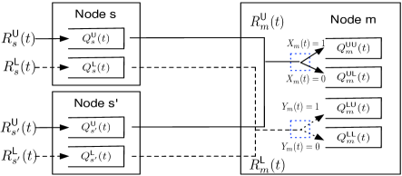
The variables Xm(t)subscript𝑋𝑚𝑡X_{m}(t) and Ym(t)subscript𝑌𝑚𝑡Y_{m}(t) are i.i.d. Bernoulli variables taking values 00 or 111 with equal probabilities, introduced for ensuring an equal division of the flow rates. Note that we have used inequality in (9). This is because the actual packet arrivals to Qm𝒯(t)superscriptsubscript𝑄𝑚𝒯𝑡Q_{m}^{{{\cal{T}}}}(t) may be less than Rm𝒯(t)superscriptsubscript𝑅𝑚𝒯𝑡R_{m}^{{{\cal{T}}}}(t) as the upstream nodes may not have enough packets to fulfill the allocated transmission rates. Our queueing structure and traffic splitting scheme are demonstrated in Fig. 5.
Refer to caption
Figure 5: The queueing structure and traffic splitting method.

IV-C3 Partition nodes in the fictitious system

Each node m𝒞n𝑚subscript𝒞𝑛m\in{{\cal{C}}}_{n} maintains only two queues QmD1(t)superscriptsubscript𝑄𝑚subscript𝐷1𝑡Q_{m}^{D_{1}}(t) and QmD2(t)superscriptsubscript𝑄𝑚subscript𝐷2𝑡Q_{m}^{D_{2}}(t) with the following dynamics:

QmDi(t+1)[QmDi(t)μm,Di(t)]++RmDi(t).superscriptsubscript𝑄𝑚subscript𝐷𝑖𝑡1superscriptdelimited-[]superscriptsubscript𝑄𝑚subscript𝐷𝑖𝑡subscript𝜇𝑚subscript𝐷𝑖𝑡superscriptsubscript𝑅𝑚subscript𝐷𝑖𝑡\displaystyle Q_{m}^{D_{i}}(t+1)\leq\big{[}Q_{m}^{D_{i}}(t)-\mu_{m,D_{i}}(t)\big{]}^{+}+R_{m}^{D_{i}}(t). (14)

Here RmD1(t)=RmU(t)superscriptsubscript𝑅𝑚subscript𝐷1𝑡superscriptsubscript𝑅𝑚U𝑡R_{m}^{D_{1}}(t)=R_{m}^{\textsf{U}}(t) and RmD2(t)=RmL(t)superscriptsubscript𝑅𝑚subscript𝐷2𝑡superscriptsubscript𝑅𝑚L𝑡R_{m}^{D_{2}}(t)=R_{m}^{\textsf{L}}(t) are the aggregate arrivals defined in (12) and (13).

IV-C4 Nodes in columns n𝑛n to 2n12𝑛12n-1 in the physical system

Each node mj=n2n1𝒞j𝑚superscriptsubscript𝑗𝑛2𝑛1subscript𝒞𝑗m\in\cup_{j=n}^{2n-1}{{\cal{C}}}_{j} maintains two First-In-First-Out (FIFO) queues Qma(t)subscriptsuperscript𝑄𝑎𝑚𝑡Q^{a}_{m}(t) and Qmb(t)subscriptsuperscript𝑄𝑏𝑚𝑡Q^{b}_{m}(t), one for the upper output link a𝑎a and the other for the lower output link b𝑏b (see Fig. 2(a)). The arrivals are placed into the queues according to their destinations, i.e.,

Qma(t+1)=[Qma(t)μm,mu(t)]++mmμm,ma(t),subscriptsuperscript𝑄𝑎𝑚𝑡1superscriptdelimited-[]subscriptsuperscript𝑄𝑎𝑚𝑡subscript𝜇𝑚subscript𝑚𝑢𝑡subscriptsuperscript𝑚subscript𝑚subscriptsuperscript𝜇𝑎superscript𝑚𝑚𝑡\displaystyle Q^{a}_{m}(t+1)=\big{[}Q^{a}_{m}(t)-\mu_{m,m_{u}}(t)\big{]}^{+}+\sum_{m^{\prime}\in{{\cal{M}}}_{m}}\mu^{a}_{m^{\prime},m}(t), (15)
Qmb(t+1)=[Qmb(t)μm,ml(t)]++mmμm,mb(t).subscriptsuperscript𝑄𝑏𝑚𝑡1superscriptdelimited-[]subscriptsuperscript𝑄𝑏𝑚𝑡subscript𝜇𝑚subscript𝑚𝑙𝑡subscriptsuperscript𝑚subscript𝑚subscriptsuperscript𝜇𝑏superscript𝑚𝑚𝑡\displaystyle Q^{b}_{m}(t+1)=\big{[}Q^{b}_{m}(t)-\mu_{m,m_{l}}(t)\big{]}^{+}+\sum_{m^{\prime}\in{{\cal{M}}}_{m}}\mu^{b}_{m^{\prime},m}(t). (16)

Here μm,ma(t)=sd𝒪maμ~m,msd(t)subscriptsuperscript𝜇𝑎superscript𝑚𝑚𝑡subscript𝑠subscript𝑑superscriptsubscript𝒪𝑚𝑎superscriptsubscript~𝜇superscript𝑚𝑚𝑠𝑑𝑡\mu^{a}_{m^{\prime},m}(t)=\sum_{s}\sum_{d\in{{\cal{O}}}_{m}^{a}}\tilde{\mu}_{m^{\prime},m}^{sd}(t), where μ~m,msd(t)superscriptsubscript~𝜇superscript𝑚𝑚𝑠𝑑𝑡\tilde{\mu}_{m^{\prime},m}^{sd}(t) denotes the actual number of flow (s,d)𝑠𝑑(s,d) packets sent from msuperscript𝑚m^{\prime} to m𝑚m at time t𝑡t, and μm,mb(t)=sd𝒪mbμ~m,msd(t)subscriptsuperscript𝜇𝑏superscript𝑚𝑚𝑡subscript𝑠subscript𝑑superscriptsubscript𝒪𝑚𝑏superscriptsubscript~𝜇superscript𝑚𝑚𝑠𝑑𝑡\mu^{b}_{m^{\prime},m}(t)=\sum_{s}\sum_{d\in{{\cal{O}}}_{m}^{b}}\tilde{\mu}_{m^{\prime},m}^{sd}(t) denotes the number of packets that need to traverse the lower outgoing link b𝑏b to their destinations.

Notice that in both systems, each partition node only maintains two queues and does not further split the traffic. This is because in the fictitious system, the next hop nodes of a partition node are D1subscript𝐷1D_{1} and D2subscript𝐷2D_{2}, whereas in the physical system, the flow (s,d)𝑠𝑑(s,d) packets at the partition nodes will be delivered to output server d𝑑d following a unique path according to Lemma 1.

We now show that under the special structure of the Benes network, our queueing structure and traffic splitting scheme generate a balanced routing across the network. This is summarized in the following lemma, where, for 𝒯ΩB𝒯subscriptΩ𝐵{{\cal{T}}}\in\Omega_{B}, we use μ¯m,m(𝒯)𝒯superscriptsubscript¯𝜇𝑚𝑚𝒯𝒯\overline{\mu}_{m,m({{\cal{T}}})}^{{{\cal{T}}}} to denote the time average transmission rates of the type 𝒯𝒯{{\cal{T}}} traffic from m𝑚m to m(𝒯)𝑚𝒯m({{\cal{T}}}). Specifically,

μ¯m,m(𝒯)𝒯limT1Tt=0T1𝔼[μ~m,m(𝒯)𝒯(t)].superscriptsubscript¯𝜇𝑚𝑚𝒯𝒯subscript𝑇1𝑇superscriptsubscript𝑡0𝑇1𝔼delimited-[]superscriptsubscript~𝜇𝑚𝑚𝒯𝒯𝑡\displaystyle\overline{\mu}_{m,m({{\cal{T}}})}^{{{\cal{T}}}}\triangleq\lim_{T\rightarrow\infty}\frac{1}{T}\sum_{t=0}^{T-1}\mathbb{E}\big{[}\tilde{\mu}_{m,m({{\cal{T}}})}^{{{\cal{T}}}}(t)\big{]}.

Here μ~m,m(𝒯)𝒯(t)superscriptsubscript~𝜇𝑚𝑚𝒯𝒯𝑡\tilde{\mu}_{m,m({{\cal{T}}})}^{{{\cal{T}}}}(t) denotes the actual number of type 𝒯𝒯{{\cal{T}}} packets sent over the link [m,m(𝒯)]𝑚𝑚𝒯[m,m({{\cal{T}}})] at time t𝑡t. Similarly, we use μ¯msdsubscriptsuperscript¯𝜇𝑠𝑑𝑚\overline{\mu}^{sd}_{m} to denote the average rate of the flow (s,d)𝑠𝑑(s,d) packets going through a node m𝑚m, i.e.,

μ¯msdlimT1Tt=0T1𝔼[μ~m,musd(t)+μ~m,mlsd(t)],subscriptsuperscript¯𝜇𝑠𝑑𝑚subscript𝑇1𝑇superscriptsubscript𝑡0𝑇1𝔼delimited-[]superscriptsubscript~𝜇𝑚subscript𝑚𝑢𝑠𝑑𝑡superscriptsubscript~𝜇𝑚subscript𝑚𝑙𝑠𝑑𝑡\displaystyle\overline{\mu}^{sd}_{m}\triangleq\lim_{T\rightarrow\infty}\frac{1}{T}\sum_{t=0}^{T-1}\mathbb{E}\big{[}\tilde{\mu}_{m,m_{u}}^{sd}(t)+\tilde{\mu}_{m,m_{l}}^{sd}(t)\big{]},

where μ~m,musd(t)superscriptsubscript~𝜇𝑚subscript𝑚𝑢𝑠𝑑𝑡\tilde{\mu}_{m,m_{u}}^{sd}(t) and μ~m,mlsd(t)superscriptsubscript~𝜇𝑚subscript𝑚𝑙𝑠𝑑𝑡\tilde{\mu}_{m,m_{l}}^{sd}(t) denote the actual numbers of flow (s,d)𝑠𝑑(s,d) packets sent from node m𝑚m to node musubscript𝑚𝑢m_{u} and node mlsubscript𝑚𝑙m_{l} at time t𝑡t, respectively.

Lemma 2

If the fictitious network is stable, then,

  • (a)

    For every node mj=1n1𝒞j𝑚superscriptsubscript𝑗1𝑛1subscript𝒞𝑗m\in\cup_{j=1}^{n-1}{{\cal{C}}}_{j},

    μ¯m,muUU=μ¯m,mlUL,μ¯m,muLU=μ¯m,mlLL.formulae-sequencesuperscriptsubscript¯𝜇𝑚subscript𝑚𝑢UUsuperscriptsubscript¯𝜇𝑚subscript𝑚𝑙ULsuperscriptsubscript¯𝜇𝑚subscript𝑚𝑢LUsuperscriptsubscript¯𝜇𝑚subscript𝑚𝑙LL\displaystyle\overline{\mu}_{m,m_{u}}^{\textsf{UU}}=\overline{\mu}_{m,m_{l}}^{\textsf{UL}},\overline{\mu}_{m,m_{u}}^{\textsf{LU}}=\overline{\mu}_{m,m_{l}}^{\textsf{LL}}. (17)
  • (b)

    The average rate of any (s,d)𝑠𝑑(s,d) flow packets going through any partition node m𝒞n𝑚subscript𝒞𝑛m\in{{\cal{C}}}_{n} satisfies μ¯msd=rsd/2n1subscriptsuperscript¯𝜇𝑠𝑑𝑚subscript𝑟𝑠𝑑superscript2𝑛1\overline{\mu}^{sd}_{m}=r_{sd}/2^{n-1}. \Diamond

Proof:

See Appendix A. ∎

IV-D The arrival admission queue

Since the arrivals to the network are dynamic, in order to perform packet admission in a fair manner, we introduce an auxiliary variables γsd(t)subscript𝛾𝑠𝑑𝑡\gamma_{sd}(t) and create the following virtual admission queue for every flow (s,d)𝑠𝑑(s,d):

Hsd(t+1)=[Hsd(t)Rsd(t)]++γsd(t).subscript𝐻𝑠𝑑𝑡1superscriptdelimited-[]subscript𝐻𝑠𝑑𝑡subscript𝑅𝑠𝑑𝑡subscript𝛾𝑠𝑑𝑡\displaystyle H_{sd}(t+1)=\big{[}H_{sd}(t)-R_{sd}(t)\big{]}^{+}+\gamma_{sd}(t). (18)

Intuitively, γsd(t)subscript𝛾𝑠𝑑𝑡\gamma_{sd}(t) indicates how many flow (s,d)𝑠𝑑(s,d) packets should have been admitted into the network. However, due to the randomness of the arrivals, this may not be feasible at every time t𝑡t. Hence, the admission queue Hsd(t)subscript𝐻𝑠𝑑𝑡H_{sd}(t) is created to ensure that in the long run, the admitted packets have a rate that is no smaller than the rate they should have got.

IV-E The output regulation queue

Here we specify the last component needed for our algorithm. Note that the above subsections have been dealing with reducing the number of queues per node and balancing the traffic inside the Benes network. In order to guarantee stability of the network, one also needs to ensure that the total traffic going to any output port of the Benes network does not exceed its capacity. To do so, we create the following regulation queue for each output port d{1,,2n}𝑑1superscript2𝑛d\in\{1,...,2^{n}\} (or equivalently, output server d𝑑d):

qd(t+1)=[qd(t)(1η)]++sRsd(t).subscript𝑞𝑑𝑡1superscriptdelimited-[]subscript𝑞𝑑𝑡1𝜂subscript𝑠subscript𝑅𝑠𝑑𝑡\displaystyle q_{d}(t+1)=\big{[}q_{d}(t)-(1-\eta)\big{]}^{+}+\sum_{s}R_{sd}(t). (19)

That is, the input to this queue are all the admitted packets destined for output port d𝑑d, and the service rate of the queue is 1η1𝜂1-\eta for some small η>0𝜂0\eta>0 for all time. The intuition here is that if these virtual queues are stable, then the average traffic rate for any output port is no more than 1η1𝜂1-\eta. The reason we have a small η𝜂\eta “slack” is to ensure queue stability for the nodes in columns n𝑛n to 2n12𝑛12n-1 in the physical network.

V The Grouped-Backpressure algorithm (G-BP)

In this section, we present the construction of the G-BP algorithm and its performance.

V-A Constructing G-BP

For notation purposes, we first define the aggregate network queue vector of the fictitious network as follows:

𝒁(t)=(Qs𝒯(t),s,𝒯Ωs,Qm𝒯(t),mj=1n1𝒞j,𝒯ΩB,\displaystyle{\boldsymbol{Z}}(t)=\big{(}Q_{s}^{{{\cal{T}}}}(t),\,\forall\,s,\,{{\cal{T}}}\in\Omega_{s},\,Q_{m}^{{{\cal{T}}}}(t),\forall\,m\in\cup_{j=1}^{n-1}{{\cal{C}}}_{j},\,{{\cal{T}}}\in\Omega_{B},
QmD1(t),QmD2(t),m𝒞n,Hsd(t),(s,d),qd(t),d).\displaystyle\qquad Q_{m}^{D_{1}}(t),Q_{m}^{D_{2}}(t),\,\forall\,m\in{{\cal{C}}}_{n},\,H_{sd}(t),\,\forall\,(s,d),\,q_{d}(t),\forall\,d\big{)}.

Then, we define the following Lyapunov function:

L(t)12s,𝒯Ωs[Qs𝒯(t)]2+12mj=1n1𝒞j𝒯ΩB[Qm𝒯(t)]2𝐿𝑡12subscript𝑠𝒯subscriptΩ𝑠superscriptdelimited-[]superscriptsubscript𝑄𝑠𝒯𝑡212subscript𝑚superscriptsubscript𝑗1𝑛1subscript𝒞𝑗subscript𝒯subscriptΩ𝐵superscriptdelimited-[]superscriptsubscript𝑄𝑚𝒯𝑡2\displaystyle L(t)\triangleq\frac{1}{2}\sum_{s,{{\cal{T}}}\in\Omega_{s}}[Q_{s}^{{{\cal{T}}}}(t)]^{2}+\frac{1}{2}\sum_{m\in\cup_{j=1}^{n-1}{{\cal{C}}}_{j}}\sum_{{{\cal{T}}}\in\Omega_{B}}[Q_{m}^{{{\cal{T}}}}(t)]^{2} (20)
+12m𝒞ni=1,2[QmDi(t)]2+12s,d[Hsd(t)]2+12d[qd(t)]2.12subscript𝑚subscript𝒞𝑛subscript𝑖12superscriptdelimited-[]superscriptsubscript𝑄𝑚subscript𝐷𝑖𝑡212subscript𝑠𝑑superscriptdelimited-[]subscript𝐻𝑠𝑑𝑡212subscript𝑑superscriptdelimited-[]subscript𝑞𝑑𝑡2\displaystyle\quad+\frac{1}{2}\sum_{m\in{{\cal{C}}}_{n}}\sum_{i=1,2}[Q_{m}^{D_{i}}(t)]^{2}+\frac{1}{2}\sum_{s,d}[H_{sd}(t)]^{2}+\frac{1}{2}\sum_{d}[q_{d}(t)]^{2}.

Now define a Lyapunov drift as follows:

Δ(t)𝔼[L(t+1)L(t)|𝒁(t)].Δ𝑡𝔼delimited-[]𝐿𝑡1conditional𝐿𝑡𝒁𝑡\displaystyle\Delta(t)\triangleq\mathbb{E}\bigg{[}L(t+1)-L(t)\left.|\right.{\boldsymbol{Z}}(t)\bigg{]}. (21)

Using the facts that 0Asd(t)Amax0subscript𝐴𝑠𝑑𝑡subscript𝐴0\leq A_{sd}(t)\leq A_{\max} and that all the link capacities in the network are bounded, we get the following lemma for the drift. In the lemma, the parameter V1𝑉1V\geq 1 is a control parameter offered by the algorithm to control the flow utility performance.

Lemma 3

Under any control policy, the following property holds for the drift at any time t𝑡t:

Δ(t)V𝔼[s,dUsd(γsd(t))|𝒁(t)]Δ𝑡𝑉𝔼delimited-[]conditionalsubscript𝑠𝑑subscript𝑈𝑠𝑑subscript𝛾𝑠𝑑𝑡𝒁𝑡\displaystyle\Delta(t)-V\mathbb{E}\bigg{[}\sum_{s,d}U_{sd}(\gamma_{sd}(t))\left.|\right.{\boldsymbol{Z}}(t)\bigg{]} (22)
Bdqd(t)(1η)m𝒞n,iQmDi(t)𝔼[μm,Di(t)|𝒁(t)]absent𝐵subscript𝑑subscript𝑞𝑑𝑡1𝜂subscript𝑚subscript𝒞𝑛𝑖superscriptsubscript𝑄𝑚subscript𝐷𝑖𝑡𝔼delimited-[]conditionalsubscript𝜇𝑚subscript𝐷𝑖𝑡𝒁𝑡\displaystyle\leq B-\sum_{d}q_{d}(t)(1-\eta)-\sum_{m\in{{\cal{C}}}_{n},i}Q_{m}^{D_{i}}(t)\mathbb{E}\bigg{[}\mu_{m,D_{i}}(t)\left.|\right.{\boldsymbol{Z}}(t)\bigg{]}
s,d𝔼[VUsd(γsd(t))Hsd(t)γsd(t)|𝒁(t)]subscript𝑠𝑑𝔼delimited-[]𝑉subscript𝑈𝑠𝑑subscript𝛾𝑠𝑑𝑡conditionalsubscript𝐻𝑠𝑑𝑡subscript𝛾𝑠𝑑𝑡𝒁𝑡\displaystyle\qquad-\sum_{s,d}\mathbb{E}\bigg{[}VU_{sd}(\gamma_{sd}(t))-H_{sd}(t)\gamma_{sd}(t)\left.|\right.{\boldsymbol{Z}}(t)\bigg{]}
sd2n1𝔼[Rsd(t)[Hsd(t)qd(t)QsU(t)]|𝒁(t)]subscript𝑠subscript𝑑superscript2𝑛1𝔼delimited-[]conditionalsubscript𝑅𝑠𝑑𝑡delimited-[]subscript𝐻𝑠𝑑𝑡subscript𝑞𝑑𝑡superscriptsubscript𝑄𝑠U𝑡𝒁𝑡\displaystyle\qquad-\sum_{s}\sum_{d\leq 2^{n-1}}\mathbb{E}\bigg{[}R_{sd}(t)\big{[}H_{sd}(t)-q_{d}(t)-Q_{s}^{\textsf{U}}(t)\big{]}\left.|\right.{\boldsymbol{Z}}(t)\bigg{]}
sd>2n1𝔼[Rsd(t)[Hsd(t)qd(t)QsL(t)]|𝒁(t)]subscript𝑠subscript𝑑superscript2𝑛1𝔼delimited-[]conditionalsubscript𝑅𝑠𝑑𝑡delimited-[]subscript𝐻𝑠𝑑𝑡subscript𝑞𝑑𝑡superscriptsubscript𝑄𝑠L𝑡𝒁𝑡\displaystyle\qquad-\sum_{s}\sum_{d>2^{n-1}}\mathbb{E}\bigg{[}R_{sd}(t)\big{[}H_{sd}(t)-q_{d}(t)-Q_{s}^{\textsf{L}}(t)\big{]}\left.|\right.{\boldsymbol{Z}}(t)\bigg{]}
s𝔼[μs,m(s)U(t)[QsU(t)12Qm(s)UU(t)12Qm(s)UL(t)]|𝒁(t)]subscript𝑠𝔼delimited-[]conditionalsuperscriptsubscript𝜇𝑠𝑚𝑠U𝑡delimited-[]superscriptsubscript𝑄𝑠U𝑡12subscriptsuperscript𝑄UU𝑚𝑠𝑡12subscriptsuperscript𝑄UL𝑚𝑠𝑡𝒁𝑡\displaystyle-\sum_{s}\mathbb{E}\bigg{[}\mu_{s,m(s)}^{\textsf{U}}(t)\big{[}Q_{s}^{\textsf{U}}(t)-\frac{1}{2}Q^{\textsf{UU}}_{m(s)}(t)-\frac{1}{2}Q^{\textsf{UL}}_{m(s)}(t)\big{]}\left.|\right.{\boldsymbol{Z}}(t)\bigg{]}
s𝔼[μs,m(s)L(t)[QsL(t)12Qm(s)LU(t)12Qm(s)LL(t)]|𝒁(t)]subscript𝑠𝔼delimited-[]conditionalsuperscriptsubscript𝜇𝑠𝑚𝑠L𝑡delimited-[]superscriptsubscript𝑄𝑠L𝑡12subscriptsuperscript𝑄LU𝑚𝑠𝑡12subscriptsuperscript𝑄LL𝑚𝑠𝑡𝒁𝑡\displaystyle-\sum_{s}\mathbb{E}\bigg{[}\mu_{s,m(s)}^{\textsf{L}}(t)\big{[}Q_{s}^{\textsf{L}}(t)-\frac{1}{2}Q^{\textsf{LU}}_{m(s)}(t)-\frac{1}{2}Q^{\textsf{LL}}_{m(s)}(t)\big{]}\left.|\right.{\boldsymbol{Z}}(t)\bigg{]}
m𝒞n1𝒯{UU, UL}𝔼[μm,m(𝒯)𝒯(t)[Qm𝒯(t)Qm(𝒯)D1(t)]|𝒁(t)]subscript𝑚subscript𝒞𝑛1subscript𝒯UU, UL𝔼delimited-[]conditionalsubscriptsuperscript𝜇𝒯𝑚𝑚𝒯𝑡delimited-[]superscriptsubscript𝑄𝑚𝒯𝑡subscriptsuperscript𝑄subscript𝐷1𝑚𝒯𝑡𝒁𝑡\displaystyle-\sum_{m\in{{\cal{C}}}_{n-1}}\sum_{{{\cal{T}}}\in\{\textsf{UU, UL}\}}\mathbb{E}\bigg{[}\mu^{{{\cal{T}}}}_{m,m({{\cal{T}}})}(t)\big{[}Q_{m}^{{{\cal{T}}}}(t)-Q^{D_{1}}_{m({{\cal{T}}})}(t)\big{]}\left.|\right.{\boldsymbol{Z}}(t)\bigg{]}
m𝒞n1𝒯{LU, LL}𝔼[μm,m(𝒯)𝒯(t)[Qm𝒯(t)Qm(𝒯)D2(t)]|𝒁(t)]subscript𝑚subscript𝒞𝑛1subscript𝒯LU, LL𝔼delimited-[]conditionalsubscriptsuperscript𝜇𝒯𝑚𝑚𝒯𝑡delimited-[]superscriptsubscript𝑄𝑚𝒯𝑡subscriptsuperscript𝑄subscript𝐷2𝑚𝒯𝑡𝒁𝑡\displaystyle-\sum_{m\in{{\cal{C}}}_{n-1}}\sum_{{{\cal{T}}}\in\{\textsf{LU, LL}\}}\mathbb{E}\bigg{[}\mu^{{{\cal{T}}}}_{m,m({{\cal{T}}})}(t)\big{[}Q_{m}^{{{\cal{T}}}}(t)-Q^{D_{2}}_{m({{\cal{T}}})}(t)\big{]}\left.|\right.{\boldsymbol{Z}}(t)\bigg{]}
mj=1n2𝒞j𝒯{UU, UL}𝔼[μm,m(𝒯)𝒯(t)[Qm𝒯(t)12Qm(𝒯)UU(t)\displaystyle-\sum_{m\in\cup_{j=1}^{n-2}{{\cal{C}}}_{j}}\sum_{{{\cal{T}}}\in\{\textsf{UU, UL}\}}\mathbb{E}\bigg{[}\mu^{{{\cal{T}}}}_{m,m({{\cal{T}}})}(t)\big{[}Q_{m}^{{{\cal{T}}}}(t)-\frac{1}{2}Q^{\textsf{UU}}_{m({{\cal{T}}})}(t)
12Qm(𝒯)UL(t)]|𝒁(t)]\displaystyle\qquad\qquad\qquad\qquad\qquad\qquad\qquad\qquad-\frac{1}{2}Q^{\textsf{UL}}_{m({{\cal{T}}})}(t)\big{]}\left.|\right.{\boldsymbol{Z}}(t)\bigg{]}
mj=1n2𝒞j𝒯{LU, LL}𝔼[μm,m(𝒯)𝒯(t)[Qm𝒯(t)12Qm(𝒯)LU(t)\displaystyle-\sum_{m\in\cup_{j=1}^{n-2}{{\cal{C}}}_{j}}\sum_{{{\cal{T}}}\in\{\textsf{LU, LL}\}}\mathbb{E}\bigg{[}\mu^{{{\cal{T}}}}_{m,m({{\cal{T}}})}(t)\big{[}Q_{m}^{{{\cal{T}}}}(t)-\frac{1}{2}Q^{\textsf{LU}}_{m({{\cal{T}}})}(t)
12Qm(𝒯)LL(t)]|𝒁(t)].\displaystyle\qquad\qquad\qquad\qquad\qquad\qquad\qquad\qquad-\frac{1}{2}Q^{\textsf{LL}}_{m({{\cal{T}}})}(t)\big{]}\left.|\right.{\boldsymbol{Z}}(t)\bigg{]}.

Here B𝐵B is a constant given by:

B=12[2n(10n2)+Amax2(23n1+22n+1+23n)],𝐵12delimited-[]superscript2𝑛10𝑛2superscriptsubscript𝐴2superscript23𝑛1superscript22𝑛1superscript23𝑛\displaystyle B=\frac{1}{2}[2^{n}(10n-2)+A_{\max}^{2}(2^{3n-1}+2^{2n+1}+2^{3n})], (23)

and the expectation is taken over the random arrivals as well as the potential randomness in the actions. \Diamond

Proof:

See Appendix B. ∎

Note that since the Benes network size is Θ(2n)Θsuperscript2𝑛\Theta(2^{n}), the n𝑛n value is only logarithmic in the network size. Hence, B𝐵B is indeed only polynomial in the network size. Based on the above lemma, we now describe our algorithm for the physical system. In the algorithm, we will operate the nodes in 𝒮𝒮{{\cal{S}}} and j=1n1𝒞jsuperscriptsubscript𝑗1𝑛1subscript𝒞𝑗\cup_{j=1}^{n-1}{{\cal{C}}}_{j} in the physical system exactly as we operate them in the fictitious system. For these nodes, the actions will be chosen in every time slot to minimize the right-hand-side (RHS) of the drift expression (22). For all the modules in columns n𝑛n to 2n12𝑛12n-1, we simply do a free-flow routing.

Grouped-Backpressure (G-BP) At every time slot t𝑡t, observe 𝑨(t)𝑨𝑡{\boldsymbol{A}}(t) and 𝒁(t)𝒁𝑡{\boldsymbol{Z}}(t), and perform the following:

  • Auxiliary Variable Selection: For every (s,d)𝑠𝑑(s,d) flow, choose γsd(t)subscript𝛾𝑠𝑑𝑡\gamma_{sd}(t) to solve:

    max::absent\displaystyle\max: VUsd(γsd(t))Hsd(t)γsd(t)𝑉subscript𝑈𝑠𝑑subscript𝛾𝑠𝑑𝑡subscript𝐻𝑠𝑑𝑡subscript𝛾𝑠𝑑𝑡\displaystyle VU_{sd}(\gamma_{sd}(t))-H_{sd}(t)\gamma_{sd}(t) (24)
    s.t. 0γsd(t)Amax.0subscript𝛾𝑠𝑑𝑡subscript𝐴\displaystyle 0\leq\gamma_{sd}(t)\leq A_{\max}.
  • Admission Control: For every input server s𝑠s: If d2n1𝑑superscript2𝑛1d\leq 2^{n-1}, choose Rsd(t)=Asd(t)subscript𝑅𝑠𝑑𝑡subscript𝐴𝑠𝑑𝑡R_{sd}(t)=A_{sd}(t) if Hsd(t)qd(t)QsU(t)>0subscript𝐻𝑠𝑑𝑡subscript𝑞𝑑𝑡superscriptsubscript𝑄𝑠U𝑡0H_{sd}(t)-q_{d}(t)-Q_{s}^{\textsf{U}}(t)>0; else choose Rsd(t)=0subscript𝑅𝑠𝑑𝑡0R_{sd}(t)=0. If d>2n1𝑑superscript2𝑛1d>2^{n-1}, choose Rsd(t)=Asd(t)subscript𝑅𝑠𝑑𝑡subscript𝐴𝑠𝑑𝑡R_{sd}(t)=A_{sd}(t) if Hsd(t)qd(t)QsL(t)>0subscript𝐻𝑠𝑑𝑡subscript𝑞𝑑𝑡superscriptsubscript𝑄𝑠L𝑡0H_{sd}(t)-q_{d}(t)-Q_{s}^{\textsf{L}}(t)>0; else choose Rsd(t)=0subscript𝑅𝑠𝑑𝑡0R_{sd}(t)=0.

  • Routing and Scheduling:

    • For any node mj=1n1𝒞j𝒮𝑚superscriptsubscript𝑗1𝑛1subscript𝒞𝑗𝒮m\in\cup_{j=1}^{n-1}{{\cal{C}}}_{j}\cup{{\cal{S}}}: define the following weights for the outgoing link [m,mu]𝑚subscript𝑚𝑢[m,m_{u}]:

      Wm,muU(t)max[QmUU(t)Q~muU(t),0],subscriptsuperscript𝑊U𝑚subscript𝑚𝑢𝑡subscriptsuperscript𝑄UU𝑚𝑡superscriptsubscript~𝑄subscript𝑚𝑢U𝑡0\displaystyle W^{\textsf{U}}_{m,m_{u}}(t)\triangleq\max\bigg{[}Q^{\textsf{UU}}_{m}(t)-\tilde{Q}_{m_{u}}^{\textsf{U}}(t),0\bigg{]}, (25)
      Wm,muL(t)max[QmLU(t)Q~muL(t),0],subscriptsuperscript𝑊L𝑚subscript𝑚𝑢𝑡subscriptsuperscript𝑄LU𝑚𝑡superscriptsubscript~𝑄subscript𝑚𝑢L𝑡0\displaystyle W^{\textsf{L}}_{m,m_{u}}(t)\triangleq\max\bigg{[}Q^{\textsf{LU}}_{m}(t)-\tilde{Q}_{m_{u}}^{\textsf{L}}(t),0\bigg{]}, (26)

      where Q~muU(t)superscriptsubscript~𝑄subscript𝑚𝑢U𝑡\tilde{Q}_{m_{u}}^{\textsf{U}}(t) and Q~muL(t)superscriptsubscript~𝑄subscript𝑚𝑢L𝑡\tilde{Q}_{m_{u}}^{\textsf{L}}(t) are defined as:

      Q~muU(t)={12QmuUU(t)+12QmuUL(t)jmn2,QmuD1(t)jm=n1,superscriptsubscript~𝑄subscript𝑚𝑢U𝑡cases12subscriptsuperscript𝑄UUsubscript𝑚𝑢𝑡12subscriptsuperscript𝑄ULsubscript𝑚𝑢𝑡subscript𝑗𝑚𝑛2subscriptsuperscript𝑄subscript𝐷1subscript𝑚𝑢𝑡subscript𝑗𝑚𝑛1\displaystyle\tilde{Q}_{m_{u}}^{\textsf{U}}(t)=\left\{\begin{array}[]{cc}\frac{1}{2}Q^{\textsf{UU}}_{m_{u}}(t)+\frac{1}{2}Q^{\textsf{UL}}_{m_{u}}(t)&j_{m}\leq n-2,\\ Q^{D_{1}}_{m_{u}}(t)&j_{m}=n-1,\end{array}\right. (29)
      Q~muL(t)={12QmuLU(t)+12QmuLL(t)jmn2,QmuD2(t)jm=n1.superscriptsubscript~𝑄subscript𝑚𝑢L𝑡cases12subscriptsuperscript𝑄LUsubscript𝑚𝑢𝑡12subscriptsuperscript𝑄LLsubscript𝑚𝑢𝑡subscript𝑗𝑚𝑛2subscriptsuperscript𝑄subscript𝐷2subscript𝑚𝑢𝑡subscript𝑗𝑚𝑛1\displaystyle\tilde{Q}_{m_{u}}^{\textsf{L}}(t)=\left\{\begin{array}[]{cc}\frac{1}{2}Q^{\textsf{LU}}_{m_{u}}(t)+\frac{1}{2}Q^{\textsf{LL}}_{m_{u}}(t)&j_{m}\leq n-2,\\ Q^{D_{2}}_{m_{u}}(t)&j_{m}=n-1.\end{array}\right. (32)

      Then, we choose the service rates μm,muUU(t)superscriptsubscript𝜇𝑚subscript𝑚𝑢UU𝑡\mu_{m,m_{u}}^{\textsf{UU}}(t) and μm,muLU(t)superscriptsubscript𝜇𝑚subscript𝑚𝑢LU𝑡\mu_{m,m_{u}}^{\textsf{LU}}(t) for link [m,mu]𝑚subscript𝑚𝑢[m,m_{u}] to solve:

      max:μm,muUU(t)Wm,muU+μm,muLU(t)Wm,muL\displaystyle\max:\quad\mu_{m,m_{u}}^{\textsf{UU}}(t)W_{m,m_{u}}^{\textsf{U}}+\mu_{m,m_{u}}^{\textsf{LU}}(t)W_{m,m_{u}}^{\textsf{L}} (33)
      s.t.μm,muUU+μm,muLU1,μm,muUU,μm,muLU{0,1}.formulae-sequences.t.superscriptsubscript𝜇𝑚subscript𝑚𝑢UUsuperscriptsubscript𝜇𝑚subscript𝑚𝑢LU1superscriptsubscript𝜇𝑚subscript𝑚𝑢UUsuperscriptsubscript𝜇𝑚subscript𝑚𝑢LU01\displaystyle\quad\text{s.t.}\quad\,\,\,\mu_{m,m_{u}}^{\textsf{UU}}+\mu_{m,m_{u}}^{\textsf{LU}}\leq 1,\,\,\mu_{m,m_{u}}^{\textsf{UU}},\mu_{m,m_{u}}^{\textsf{LU}}\in\{0,1\}.

      To solve for μm,mlUL(t)superscriptsubscript𝜇𝑚subscript𝑚𝑙UL𝑡\mu_{m,m_{l}}^{\textsf{UL}}(t) and μm,mlLL(t)superscriptsubscript𝜇𝑚subscript𝑚𝑙LL𝑡\mu_{m,m_{l}}^{\textsf{LL}}(t), we replace QmUU(t)superscriptsubscript𝑄𝑚UU𝑡Q_{m}^{\textsf{UU}}(t) and QmLU(t)superscriptsubscript𝑄𝑚LU𝑡Q_{m}^{\textsf{LU}}(t) with QmUL(t)superscriptsubscript𝑄𝑚UL𝑡Q_{m}^{\textsf{UL}}(t) and QmLL(t)superscriptsubscript𝑄𝑚LL𝑡Q_{m}^{\textsf{LL}}(t) in (25) and (26). Also, we replace musubscript𝑚𝑢m_{u} and D1subscript𝐷1D_{1} with mlsubscript𝑚𝑙m_{l} and D2subscript𝐷2D_{2} in (29) and (32). If m=s𝒮𝑚𝑠𝒮m=s\in{{\cal{S}}}, we simply replace QmUU(t)superscriptsubscript𝑄𝑚UU𝑡Q_{m}^{\textsf{UU}}(t) and QmUL(t)superscriptsubscript𝑄𝑚UL𝑡Q_{m}^{\textsf{UL}}(t) with QsU(t)superscriptsubscript𝑄𝑠U𝑡Q_{s}^{\textsf{U}}(t) and QsL(t)superscriptsubscript𝑄𝑠L𝑡Q_{s}^{\textsf{L}}(t) in (25) and (26), and replace musubscript𝑚𝑢m_{u} by m(s)𝑚𝑠m(s) in (29) and (32).

    • For every node mj=n2n1𝒞j𝑚superscriptsubscript𝑗𝑛2𝑛1subscript𝒞𝑗m\in\cup_{j=n}^{2n-1}{{\cal{C}}}_{j}: Each module serves each FIFO queue for each outgoing link according to (15) and (16) with μm,mu(t)=μm,ml(t)=1subscript𝜇𝑚subscript𝑚𝑢𝑡subscript𝜇𝑚subscript𝑚𝑙𝑡1\mu_{m,m_{u}}(t)=\mu_{m,m_{l}}(t)=1 for all time.

  • Queue Updates: In the fictitious system, choose the service rates μm,D1(t)subscript𝜇𝑚subscript𝐷1𝑡\mu_{m,D_{1}}(t) and μm,D2(t)subscript𝜇𝑚subscript𝐷2𝑡\mu_{m,D_{2}}(t) to solve:

    max::absent\displaystyle\max: QmD1(t)μm,D1(t)+QmD2(t)μm,D2(t)superscriptsubscript𝑄𝑚subscript𝐷1𝑡subscript𝜇𝑚subscript𝐷1𝑡superscriptsubscript𝑄𝑚subscript𝐷2𝑡subscript𝜇𝑚subscript𝐷2𝑡\displaystyle Q_{m}^{D_{1}}(t)\mu_{m,D_{1}}(t)+Q_{m}^{D_{2}}(t)\mu_{m,D_{2}}(t) (34)
    s.t. μm,D1(t),μm,D2(t){0,1}.subscript𝜇𝑚subscript𝐷1𝑡subscript𝜇𝑚subscript𝐷2𝑡01\displaystyle\mu_{m,D_{1}}(t),\mu_{m,D_{2}}(t)\in\{0,1\}.

    Then, update all the queues in both the fictitious system and the physical system according to their dynamics. \Diamond

We note that G-BP only controls the first half of the physical system with the backpressure actions. All the nodes in columns n𝑛n to 2n12𝑛12n-1 simply serve the flows with a “free-flow” manner, i.e., always serve the flows at the maximum rate. This is different from the usual backpressure algorithms that control all the queues in the network to ensure stability.

V-B Performance analysis

In this section, we prove that G-BP achieves a near-optimal performance. To carry out our analysis, we first have the following theorem, which characterizes the capacity region of a Benes network. In the theorem, we use 𝒓=(rsd,(s,d))𝒓subscript𝑟𝑠𝑑for-all𝑠𝑑{\boldsymbol{r}}=(r_{sd},\,\forall\,(s,d)) to denote the vector of arrival rates, where rsdsubscript𝑟𝑠𝑑r_{sd} represents the average rate of the (s,d)𝑠𝑑(s,d) flow.

Theorem 1

[8] [9] The capacity region of the Benes network 𝔹nsubscript𝔹𝑛\mathbb{B}_{n} is given by:

Λn={𝒓|s=12nrsd1,d=12nrsd1,rsd0,s,d}.formulae-sequencesubscriptΛ𝑛conditional-set𝒓formulae-sequencesuperscriptsubscript𝑠1superscript2𝑛subscript𝑟𝑠𝑑1formulae-sequencesuperscriptsubscript𝑑1superscript2𝑛subscript𝑟𝑠𝑑1subscript𝑟𝑠𝑑0for-all𝑠𝑑\displaystyle\Lambda_{n}=\{{\boldsymbol{r}}\left.|\right.\sum_{s=1}^{2^{n}}r_{sd}\leq 1,\,\sum_{d=1}^{2^{n}}r_{sd}\leq 1,\,r_{sd}\geq 0,\forall\,s,d\}.\Diamond

We now present the performance results of the G-BP algorithm. Recall that β𝛽\beta is defined in (2) to be the maximum first derivative among all utility functions, and that 𝒓optΛnsuperscript𝒓optsubscriptΛ𝑛{\boldsymbol{r}}^{\textsf{opt}}\in\Lambda_{n} denotes the optimal solution to the flow utility maximization problem.

Theorem 2

Suppose both the fictitious network and the physical network are empty at time t=0𝑡0t=0, i.e., all the queues are zero. Then, (i) Both the fictitious network and the physical network are stable under G-BP, and (ii) Denote 𝐫G-BPsuperscript𝐫G-BP{\boldsymbol{r}}^{\textsf{G-BP}} the time average rate vector achieved by G-BP. We have:

U(𝒓G-BP)U(𝒓opt)BV2nβη.\displaystyle U({\boldsymbol{r}}^{\textsf{G-BP}})\geq U({\boldsymbol{r}}^{\textsf{opt}})-\frac{B}{V}-2^{n}\beta\eta.\quad\Diamond (35)
Proof:

See Appendix C. ∎

From (35), we see that the utility performance of G-BP can arbitrarily approach the optimal as we increase V𝑉V and decrease η𝜂\eta. However, doing so will increase the average network delay. Hence, there is a natural tradeoff between the utility performance and the network delay.

Note that though the performance results in Theorem 2 look similar to previous results in [13], the proof is indeed quite different. This is because in our case, we impose a special queueing structure on the network, and the second half of the network uses a free-flow routing. These two features make the analysis very different from the usual backpressure algorithms, under which each node maintains a separate queue for each flow, and all the network actions are based on the network queue sizes.

V-C Discussion on implementation

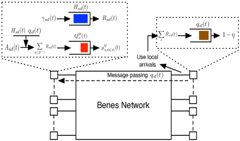
We note that the G-BP algorithm can easily be implemented in a fully distributed manner. Specifically, one can maintain the virtual admission queues at the input servers and maintain the virtual output regulation queues at the output servers using counters, as shown in Fig. 6. With this arrangement, the auxiliary variable selection step can easily be done locally at the input servers, and the routing and scheduling step can easily be done by each node exchanging queue information only with its four neighbors. The admission control step requires the input servers to know the regulation queue sizes. This can be achieved by message passing the regulating queue sizes along the network using prioritized packets. Similarly, the update of the regulation queues requires the knowledge of the arrivals for the output port. This can be approximated by using the arrivals to the output servers as the input to the regulation queues. Though message passing and queue approximation may incur performance loss in practice, we will see in the simulation section that, the G-BP algorithm is indeed very robust and can still achieve near-optimal performance even under different message passing delays and regulation queue approximation.

Finally, note that though we have described implementing our algorithm with actual data queue sizes. In practice, to further reduce network delay, we can also implement G-BP with counters to keep track of the queue processes that should have been generated for decision making, and admit slightly smaller arrival rates than G-BP.
Refer to caption
Figure 6: Implementation of G-BP. The virtual admission queues are maintained at the input servers, while the virtual regulation queues are maintained at the output servers. Message passing is used to send regulation queue information through the network for admission control. The regulation queues can use the local arrivals to the output servers as the input.

VI Simulation

In this section, we present the simulation results of G-BP on a 24×24superscript24superscript242^{4}\times 2^{4} size Benes network. For simplicity, we assume that Asd(t)=Amax=2subscript𝐴𝑠𝑑𝑡subscript𝐴2A_{sd}(t)=A_{\max}=2 for all time.

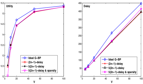
In the simulation, we assume that every flow has a utility function log(1+rsd)1subscript𝑟𝑠𝑑\log(1+r_{sd}). In every time slot, each flow can admit 00, 111 or 222 packets. We simulate the system for V{5,10,20,50,100}𝑉5102050100V\in\{5,10,20,50,100\} and η=0.01𝜂0.01\eta=0.01. Each simulation is run for 105superscript10510^{5} slots. To test the robustness of G-BP against the delay and sparsity in message passing and the regulation queue approximation, we simulate four different cases. (i) The original G-BP algorithm, where the message passing delay is zero and the regulation queue is exact. (ii) The case when the input to the regulation queue qd(t)subscript𝑞𝑑𝑡q_{d}(t) are the actual packet arrivals to the output server d𝑑d (the service rate is still 1η1𝜂1-\eta), and admission control at time t𝑡t uses qd(t(2n1))subscript𝑞𝑑𝑡2𝑛1q_{d}(t-(2n-1)) instead of qd(t)subscript𝑞𝑑𝑡q_{d}(t). (iii) Similar to the second case, but admission control at time t𝑡t uses qd(t5(2n1))subscript𝑞𝑑𝑡52𝑛1q_{d}(t-5(2n-1)). (iv) Similar to the second case, but the regulation queue information is only sent every 5(2n1)52𝑛15(2n-1) slots and has a delay of 5(2n1)52𝑛15(2n-1). That is, admission control at time t𝑡t uses qd(t0)subscript𝑞𝑑subscript𝑡0q_{d}(t_{0}) where t0=max[(t5(2n1)1)5(2n1),1]subscript𝑡0𝑡52𝑛1152𝑛11t_{0}=\max[(\lfloor\frac{t}{5(2n-1)}\rfloor-1)5(2n-1),1].

Refer to caption
Figure 7: The aggregate flow utility and average packet delay under G-BP. One can see that G-BP works very well even with message passing delay and regulation queue approximation.

Fig. 7 shows the performance of the G-BP algorithm. Here the average delay (in number of slots) is computed using the set of packets that are delivered when the simulation ends. For all simulations, this set contains more than 99.9%percent99.999.9\% of the total packets that enter the network. We see that as we increase the V𝑉V value, the aggregate flow utility quickly converges to its optimal value. However, doing so also leads to a linear increase of the average packet delay. We also see from the figure that, G-BP is indeed very robust to the delay and sparsity in message passing, and regulation queue approximation.

In Fig. 8, we plot a recorded queue process of the network under G-BP for V=10𝑉10V=10. In this case, we change each flow’s utility function to wsdlog(1+rsd)subscript𝑤𝑠𝑑1subscript𝑟𝑠𝑑w_{sd}\log(1+r_{sd}) in the middle of the simulation, where wsdsubscript𝑤𝑠𝑑w_{sd} takes values 1,2121,2 or 333 equally likely. We see that after the change, G-BP quickly adapts to the new utility functions and performs admission and routing accordingly.
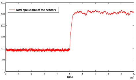
Refer to caption
Figure 8: The total network queue size under G-BP with V=10𝑉10V=10.

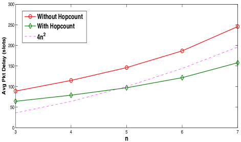
Finally, we also evaluate the average packet delay as a function of the network size, to see how the algorithm scales. As comparison, we also simulate an “enhanced” G-BP algorithm, in which we replace each queue value in the algorithm with the queue value plus the node’s hop count to the destination, i.e., its column number. The idea is to create “bias” towards the packet destinations. This enhancement is similar to the EDRPC algorithm developed in [16]. We can see from Fig. 9 that the average packet delay under G-BP scales as Θ(n2)Θsuperscript𝑛2\Theta(n^{2}). Since the Benes network size is Θ(2n)Θsuperscript2𝑛\Theta(2^{n}), this implies that the average delay grows only logarithmically in the network size.
Refer to caption
Figure 9: Average delay as a function of the network size under V=10𝑉10V=10.

Note that in Fig. 9 we have plotted the average delay in number of slots. To get some physical understanding of the results, assume that each packet has 500500500 bytes and each link has a capacity of 111 Gbit/second, which are both quite common in practice. Then, every slot is 444 microseconds. Hence, we see that the average packet delay under Benes network with G-BP is roughly 111 millisecond when the network size is 128×128128128128\times 128. This demonstrates the good delay performance of our network design approach.

VII Conclusion

In this work, we develop a novel networking solution called Benes packet network, which consists of a Benes network built with simple commodity switches, a flow utility maximization mechanism, and a Grouped-Backpressure (G-BP) routing and scheduling algorithm. We show that this combination can achieve a near-optimal flow utility and ensure small end-to-end delay for the traffic flows. Our approach also only requires each switch module to maintain at most four queues regardless of the network size, and can easily be implemented in practice in a fully distributed manner.

Appendix A – Proof of Lemma 2

Proof:

(Lemma 2) We first prove Part (a). From the queueing dynamic equation (9), we see that for any node mj=1n1𝒞j𝑚superscriptsubscript𝑗1𝑛1subscript𝒞𝑗m\in\cup_{j=1}^{n-1}{{\cal{C}}}_{j}, the input rates into QmUU(t)superscriptsubscript𝑄𝑚UU𝑡Q_{m}^{\textsf{UU}}(t) and QmUL(t)superscriptsubscript𝑄𝑚UL𝑡Q_{m}^{\textsf{UL}}(t) are equal because of random splitting. Similarly, the input rates into QmLU(t)superscriptsubscript𝑄𝑚LU𝑡Q_{m}^{\textsf{LU}}(t) and QmLL(t)superscriptsubscript𝑄𝑚LL𝑡Q_{m}^{\textsf{LL}}(t) are the same. Hence, if the fictitious network is stable, the output rates from these queues are equal to their input rates [12]. Therefore (17) holds.

Now we prove Part (b) by induction. First we see that it holds for any 4×4444\times 4 Benes network. This is because if the fictitious network is stable, then the input switch modules split the incoming flows equally into the two partition nodes (see Fig. 2).

Now suppose the same is true for a 2n1×2n1superscript2𝑛1superscript2𝑛12^{n-1}\times 2^{n-1} Benes network, we want to show that it also holds for a 2n×2nsuperscript2𝑛superscript2𝑛2^{n}\times 2^{n} Benes network.

To see this, note from Fig. 2 that each 2n×2nsuperscript2𝑛superscript2𝑛2^{n}\times 2^{n} Benes network consists of two 2n1×2n1superscript2𝑛1superscript2𝑛12^{n-1}\times 2^{n-1} subnetworks, 2n1superscript2𝑛12^{n-1} input switch modules and 2n1superscript2𝑛12^{n-1} output switch modules. According to the structure of the Benes network, any input switch module has one link connecting to the upper 2n1×2n1superscript2𝑛1superscript2𝑛12^{n-1}\times 2^{n-1} subnetwork and the other one connecting to the lower 2n1×2n1superscript2𝑛1superscript2𝑛12^{n-1}\times 2^{n-1} subnetwork. From Part (a), we see that half of a flow’s rate will be routed through the upper subnetwork and the other half will be routed through the lower subnetwork. Now consider the upper subnetwork and view the flow traffic into this subnetwork as its own external input. Since this subnetwork is also stable, the flow’s traffic will be equally split and routed via its partition nodes by induction. Since all the partition nodes coincide according to Fact 1, we see that the lemma follows. ∎

Appendix B – Proof of Lemma 3

Here we present the proof of Lemma 3.

Proof:

Squaring both sides of (7) and using the fact that for any real number x𝑥x, ([x]+)2x2superscriptsuperscriptdelimited-[]𝑥2superscript𝑥2([x]^{+})^{2}\leq x^{2}, we get for every s𝒮𝑠𝒮s\in{{\cal{S}}} and 𝒯Ωs𝒯subscriptΩ𝑠{{\cal{T}}}\in\Omega_{s} that:

[Qs𝒯(t+1)]2[Qs𝒯(t)]2+[Rs𝒯(t)]2+[μs,m(s)𝒯(t)]2superscriptdelimited-[]superscriptsubscript𝑄𝑠𝒯𝑡12superscriptdelimited-[]superscriptsubscript𝑄𝑠𝒯𝑡2superscriptdelimited-[]superscriptsubscript𝑅𝑠𝒯𝑡2superscriptdelimited-[]superscriptsubscript𝜇𝑠𝑚𝑠𝒯𝑡2\displaystyle[Q_{s}^{{{\cal{T}}}}(t+1)]^{2}\leq[Q_{s}^{{{\cal{T}}}}(t)]^{2}+[R_{s}^{{{\cal{T}}}}(t)]^{2}+[\mu_{s,m(s)}^{{{\cal{T}}}}(t)]^{2} (36)
2Qs𝒯(t)[μs,m(s)𝒯(t)Rs𝒯(t)].2superscriptsubscript𝑄𝑠𝒯𝑡delimited-[]superscriptsubscript𝜇𝑠𝑚𝑠𝒯𝑡superscriptsubscript𝑅𝑠𝒯𝑡\displaystyle-2Q_{s}^{{{\cal{T}}}}(t)[\mu_{s,m(s)}^{{{\cal{T}}}}(t)-R_{s}^{{{\cal{T}}}}(t)].

Now note that μs,m(s)𝒯(t)1superscriptsubscript𝜇𝑠𝑚𝑠𝒯𝑡1\mu_{s,m(s)}^{{{\cal{T}}}}(t)\leq 1 and Rs𝒯(t)2n1Amaxsuperscriptsubscript𝑅𝑠𝒯𝑡superscript2𝑛1subscript𝐴R_{s}^{{{\cal{T}}}}(t)\leq 2^{n-1}A_{\max}. Hence, if we define B12(2n+23n2Amax2)subscript𝐵12superscript2𝑛superscript23𝑛2subscriptsuperscript𝐴2B_{1}\triangleq 2(2^{n}+2^{3n-2}A^{2}_{\max}) and sum (36) over s𝒮𝑠𝒮s\in{{\cal{S}}} and 𝒯Ωs𝒯subscriptΩ𝑠{{\cal{T}}}\in\Omega_{s}, we have:

s𝒮,𝒯Ωs[Qs𝒯(t+1)]2s𝒮,𝒯Ωs[Qs𝒯(t)]2+B1subscriptformulae-sequence𝑠𝒮𝒯subscriptΩ𝑠superscriptdelimited-[]superscriptsubscript𝑄𝑠𝒯𝑡12subscriptformulae-sequence𝑠𝒮𝒯subscriptΩ𝑠superscriptdelimited-[]superscriptsubscript𝑄𝑠𝒯𝑡2subscript𝐵1\displaystyle\sum_{s\in{{\cal{S}}},{{\cal{T}}}\in\Omega_{s}}[Q_{s}^{{{\cal{T}}}}(t+1)]^{2}\leq\sum_{s\in{{\cal{S}}},{{\cal{T}}}\in\Omega_{s}}[Q_{s}^{{{\cal{T}}}}(t)]^{2}+B_{1}
2s𝒮,𝒯ΩsQs𝒯(t)[μs,m(s)𝒯(t)Rs𝒯(t)].2subscriptformulae-sequence𝑠𝒮𝒯subscriptΩ𝑠superscriptsubscript𝑄𝑠𝒯𝑡delimited-[]superscriptsubscript𝜇𝑠𝑚𝑠𝒯𝑡superscriptsubscript𝑅𝑠𝒯𝑡\displaystyle\qquad\qquad\qquad-2\sum_{s\in{{\cal{S}}},{{\cal{T}}}\in\Omega_{s}}Q_{s}^{{{\cal{T}}}}(t)[\mu_{s,m(s)}^{{{\cal{T}}}}(t)-R_{s}^{{{\cal{T}}}}(t)].

Using a similar argument as above, we get the following:

mj=1n1𝒞j,𝒯ΩB[Qm𝒯(t+1)]2mj=1n1𝒞j,𝒯ΩB[Qm𝒯(t)]2subscriptformulae-sequence𝑚superscriptsubscript𝑗1𝑛1subscript𝒞𝑗𝒯subscriptΩ𝐵superscriptdelimited-[]superscriptsubscript𝑄𝑚𝒯𝑡12subscriptformulae-sequence𝑚superscriptsubscript𝑗1𝑛1subscript𝒞𝑗𝒯subscriptΩ𝐵superscriptdelimited-[]superscriptsubscript𝑄𝑚𝒯𝑡2\displaystyle\sum_{m\in\cup_{j=1}^{n-1}{{\cal{C}}}_{j},{{\cal{T}}}\in\Omega_{B}}[Q_{m}^{{{\cal{T}}}}(t+1)]^{2}-\sum_{m\in\cup_{j=1}^{n-1}{{\cal{C}}}_{j},{{\cal{T}}}\in\Omega_{B}}[Q_{m}^{{{\cal{T}}}}(t)]^{2}
B22mj=1n1𝒞j,𝒯ΩBQm𝒯(t)[μm,m(𝒯)𝒯(t)Rm𝒯(t)].absentsubscript𝐵22subscriptformulae-sequence𝑚superscriptsubscript𝑗1𝑛1subscript𝒞𝑗𝒯subscriptΩ𝐵superscriptsubscript𝑄𝑚𝒯𝑡delimited-[]superscriptsubscript𝜇𝑚𝑚𝒯𝒯𝑡superscriptsubscript𝑅𝑚𝒯𝑡\displaystyle\leq B_{2}-2\sum_{m\in\cup_{j=1}^{n-1}{{\cal{C}}}_{j},{{\cal{T}}}\in\Omega_{B}}Q_{m}^{{{\cal{T}}}}(t)[\mu_{m,m({{\cal{T}}})}^{{{\cal{T}}}}(t)-R_{m}^{{{\cal{T}}}}(t)].

Here B220(n1)2n1subscript𝐵220𝑛1superscript2𝑛1B_{2}\triangleq 20(n-1)2^{n-1}. Now repeat the above for all the other queues in the fictitious system, we will also get:

m𝒞n,i[QmDi(t+1)]2m𝒞n,i[QmDi(t)]2subscript𝑚subscript𝒞𝑛𝑖superscriptdelimited-[]superscriptsubscript𝑄𝑚subscript𝐷𝑖𝑡12subscript𝑚subscript𝒞𝑛𝑖superscriptdelimited-[]superscriptsubscript𝑄𝑚subscript𝐷𝑖𝑡2\displaystyle\sum_{m\in{{\cal{C}}}_{n},i}[Q_{m}^{D_{i}}(t+1)]^{2}-\sum_{m\in{{\cal{C}}}_{n},i}[Q_{m}^{D_{i}}(t)]^{2}
B32m𝒞n,iQmDi(t)[μm,Di(t)RmDi(t)],absentsubscript𝐵32subscript𝑚subscript𝒞𝑛𝑖superscriptsubscript𝑄𝑚subscript𝐷𝑖𝑡delimited-[]subscript𝜇𝑚subscript𝐷𝑖𝑡subscriptsuperscript𝑅subscript𝐷𝑖𝑚𝑡\displaystyle\qquad\qquad\qquad\leq B_{3}-2\sum_{m\in{{\cal{C}}}_{n},i}Q_{m}^{D_{i}}(t)[\mu_{m,D_{i}}(t)-R^{D_{i}}_{m}(t)],
s,d[Hsd(t+1)]2s,d[Hsd(t)]2subscript𝑠𝑑superscriptdelimited-[]subscript𝐻𝑠𝑑𝑡12subscript𝑠𝑑superscriptdelimited-[]subscript𝐻𝑠𝑑𝑡2\displaystyle\sum_{s,d}[H_{sd}(t+1)]^{2}-\sum_{s,d}[H_{sd}(t)]^{2}
B42s,dHsd(t)[Rsd(t)γsd(t)],absentsubscript𝐵42subscript𝑠𝑑subscript𝐻𝑠𝑑𝑡delimited-[]subscript𝑅𝑠𝑑𝑡subscript𝛾𝑠𝑑𝑡\displaystyle\qquad\qquad\qquad\leq B_{4}-2\sum_{s,d}H_{sd}(t)[R_{sd}(t)-\gamma_{sd}(t)],
d[qd(t+1)]2d[qd(t)]2subscript𝑑superscriptdelimited-[]subscript𝑞𝑑𝑡12subscript𝑑superscriptdelimited-[]subscript𝑞𝑑𝑡2\displaystyle\sum_{d}[q_{d}(t+1)]^{2}-\sum_{d}[q_{d}(t)]^{2}
B52dqd(t)[1ηsRsd(t)].absentsubscript𝐵52subscript𝑑subscript𝑞𝑑𝑡delimited-[]1𝜂subscript𝑠subscript𝑅𝑠𝑑𝑡\displaystyle\qquad\qquad\qquad\leq B_{5}-2\sum_{d}q_{d}(t)[1-\eta-\sum_{s}R_{sd}(t)].

Here B3=52nsubscript𝐵35superscript2𝑛B_{3}=5\cdot 2^{n}, B4=22n+1Amax2subscript𝐵4superscript22𝑛1superscriptsubscript𝐴2B_{4}=2^{2n+1}A_{\max}^{2} and B5=2n+23nAmax2subscript𝐵5superscript2𝑛superscript23𝑛superscriptsubscript𝐴2B_{5}=2^{n}+2^{3n}A_{\max}^{2}.

Summing all the resulting inequalities, multiplying both sides by 1212\frac{1}{2} and taking expectations on both sides conditioning on 𝒁(t)𝒁𝑡{\boldsymbol{Z}}(t), we obtain the following:

Δ(t)BΔ𝑡𝐵\displaystyle\Delta(t)\leq B (37)
s𝒮𝒯ΩsQs𝒯(t)𝔼[μs,m(s)𝒯(t)Rs𝒯(t)|𝒁(t)]subscript𝑠𝒮subscript𝒯subscriptΩ𝑠superscriptsubscript𝑄𝑠𝒯𝑡𝔼delimited-[]superscriptsubscript𝜇𝑠𝑚𝑠𝒯𝑡conditionalsuperscriptsubscript𝑅𝑠𝒯𝑡𝒁𝑡\displaystyle-\sum_{s\in{{\cal{S}}}}\sum_{{{\cal{T}}}\in\Omega_{s}}Q_{s}^{{{\cal{T}}}}(t)\mathbb{E}\bigg{[}\mu_{s,m(s)}^{{{\cal{T}}}}(t)-R_{s}^{{{\cal{T}}}}(t)\left.|\right.{\boldsymbol{Z}}(t)\bigg{]}
mj=1n1𝒞j𝒯ΩBQm𝒯(t)𝔼[μm,m(𝒯)𝒯(t)Rm𝒯(t)|𝒁(t)]subscript𝑚superscriptsubscript𝑗1𝑛1subscript𝒞𝑗subscript𝒯subscriptΩ𝐵superscriptsubscript𝑄𝑚𝒯𝑡𝔼delimited-[]superscriptsubscript𝜇𝑚𝑚𝒯𝒯𝑡conditionalsuperscriptsubscript𝑅𝑚𝒯𝑡𝒁𝑡\displaystyle-\sum_{m\in\cup_{j=1}^{n-1}{{\cal{C}}}_{j}}\sum_{{{\cal{T}}}\in\Omega_{B}}Q_{m}^{{{\cal{T}}}}(t)\mathbb{E}\bigg{[}\mu_{m,m({{\cal{T}}})}^{{{\cal{T}}}}(t)-R_{m}^{{{\cal{T}}}}(t)\left.|\right.{\boldsymbol{Z}}(t)\bigg{]}
m𝒞ni=1,2QmDi(t)𝔼[μm,Di(t)RmDi(t)|𝒁(t)]subscript𝑚subscript𝒞𝑛subscript𝑖12superscriptsubscript𝑄𝑚subscript𝐷𝑖𝑡𝔼delimited-[]subscript𝜇𝑚subscript𝐷𝑖𝑡conditionalsuperscriptsubscript𝑅𝑚subscript𝐷𝑖𝑡𝒁𝑡\displaystyle\qquad-\sum_{m\in{{\cal{C}}}_{n}}\sum_{i=1,2}Q_{m}^{D_{i}}(t)\mathbb{E}\bigg{[}\mu_{m,D_{i}}(t)-R_{m}^{D_{i}}(t)\left.|\right.{\boldsymbol{Z}}(t)\bigg{]}
s,dHsd(t)𝔼[Rsd(t)γsd(t)|𝒁(t)]subscript𝑠𝑑subscript𝐻𝑠𝑑𝑡𝔼delimited-[]subscript𝑅𝑠𝑑𝑡conditionalsubscript𝛾𝑠𝑑𝑡𝒁𝑡\displaystyle\qquad-\sum_{s,d}H_{sd}(t)\mathbb{E}\bigg{[}R_{sd}(t)-\gamma_{sd}(t)\left.|\right.{\boldsymbol{Z}}(t)\bigg{]}
dqd(t)𝔼[1ηsRsd(t)|𝒁(t)].subscript𝑑subscript𝑞𝑑𝑡𝔼delimited-[]1𝜂conditionalsubscript𝑠subscript𝑅𝑠𝑑𝑡𝒁𝑡\displaystyle\qquad-\sum_{d}q_{d}(t)\mathbb{E}\bigg{[}1-\eta-\sum_{s}R_{sd}(t)\left.|\right.{\boldsymbol{Z}}(t)\bigg{]}.

Here the constant B12i=1,,5Bi𝐵12subscript𝑖15subscript𝐵𝑖B\triangleq\frac{1}{2}\sum_{i=1,...,5}B_{i}, i.e.,

B=12[2n(10n2)+Amax2(23n1+22n+1+23n)].𝐵12delimited-[]superscript2𝑛10𝑛2superscriptsubscript𝐴2superscript23𝑛1superscript22𝑛1superscript23𝑛\displaystyle B=\frac{1}{2}[2^{n}(10n-2)+A_{\max}^{2}(2^{3n-1}+2^{2n+1}+2^{3n})]. (38)

Now by adding to both sides of (37) the term V𝔼[sdUsd(γsd(t))|𝒁(t)]𝑉𝔼delimited-[]conditionalsubscript𝑠𝑑subscript𝑈𝑠𝑑subscript𝛾𝑠𝑑𝑡𝒁𝑡-V\mathbb{E}\big{[}\sum_{sd}U_{sd}(\gamma_{sd}(t))\left.|\right.{\boldsymbol{Z}}(t)\big{]}, we get:

Δ(t)V𝔼[s,dUsd(γsd(t))|𝒁(t)]Δ𝑡𝑉𝔼delimited-[]conditionalsubscript𝑠𝑑subscript𝑈𝑠𝑑subscript𝛾𝑠𝑑𝑡𝒁𝑡\displaystyle\Delta(t)-V\mathbb{E}\bigg{[}\sum_{s,d}U_{sd}(\gamma_{sd}(t))\left.|\right.{\boldsymbol{Z}}(t)\bigg{]} (39)
Bs𝒯ΩsQs𝒯(t)𝔼[μs,m(s)𝒯(t)Rs𝒯(t)|𝒁(t)]absent𝐵subscript𝑠subscript𝒯subscriptΩ𝑠superscriptsubscript𝑄𝑠𝒯𝑡𝔼delimited-[]superscriptsubscript𝜇𝑠𝑚𝑠𝒯𝑡conditionalsuperscriptsubscript𝑅𝑠𝒯𝑡𝒁𝑡\displaystyle\leq B-\sum_{s}\sum_{{{\cal{T}}}\in\Omega_{s}}Q_{s}^{{{\cal{T}}}}(t)\mathbb{E}\bigg{[}\mu_{s,m(s)}^{{{\cal{T}}}}(t)-R_{s}^{{{\cal{T}}}}(t)\left.|\right.{\boldsymbol{Z}}(t)\bigg{]}
mj=1n1𝒞j𝒯ΩBQm𝒯(t)𝔼[μm,m(𝒯)𝒯(t)Rm𝒯(t)|𝒁(t)]subscript𝑚superscriptsubscript𝑗1𝑛1subscript𝒞𝑗subscript𝒯subscriptΩ𝐵superscriptsubscript𝑄𝑚𝒯𝑡𝔼delimited-[]superscriptsubscript𝜇𝑚𝑚𝒯𝒯𝑡conditionalsuperscriptsubscript𝑅𝑚𝒯𝑡𝒁𝑡\displaystyle-\sum_{m\in\cup_{j=1}^{n-1}{{\cal{C}}}_{j}}\sum_{{{\cal{T}}}\in\Omega_{B}}Q_{m}^{{{\cal{T}}}}(t)\mathbb{E}\bigg{[}\mu_{m,m({{\cal{T}}})}^{{{\cal{T}}}}(t)-R_{m}^{{{\cal{T}}}}(t)\left.|\right.{\boldsymbol{Z}}(t)\bigg{]}
m𝒞ni=1,2QmDi(t)𝔼[μm,Di(t)RmDi(t)|𝒁(t)]subscript𝑚subscript𝒞𝑛subscript𝑖12superscriptsubscript𝑄𝑚subscript𝐷𝑖𝑡𝔼delimited-[]subscript𝜇𝑚subscript𝐷𝑖𝑡conditionalsuperscriptsubscript𝑅𝑚subscript𝐷𝑖𝑡𝒁𝑡\displaystyle\qquad-\sum_{m\in{{\cal{C}}}_{n}}\sum_{i=1,2}Q_{m}^{D_{i}}(t)\mathbb{E}\bigg{[}\mu_{m,D_{i}}(t)-R_{m}^{D_{i}}(t)\left.|\right.{\boldsymbol{Z}}(t)\bigg{]}
V𝔼[s,dUsd(γsd(t))|𝒁(t)]𝑉𝔼delimited-[]conditionalsubscript𝑠𝑑subscript𝑈𝑠𝑑subscript𝛾𝑠𝑑𝑡𝒁𝑡\displaystyle\qquad-V\mathbb{E}\bigg{[}\sum_{s,d}U_{sd}(\gamma_{sd}(t))\left.|\right.{\boldsymbol{Z}}(t)\bigg{]}
s,dHsd(t)𝔼[Rsd(t)γsd(t)|𝒁(t)]subscript𝑠𝑑subscript𝐻𝑠𝑑𝑡𝔼delimited-[]subscript𝑅𝑠𝑑𝑡conditionalsubscript𝛾𝑠𝑑𝑡𝒁𝑡\displaystyle\qquad-\sum_{s,d}H_{sd}(t)\mathbb{E}\bigg{[}R_{sd}(t)-\gamma_{sd}(t)\left.|\right.{\boldsymbol{Z}}(t)\bigg{]}
dqd(t)𝔼[1ηsRsd(t)|𝒁(t)].subscript𝑑subscript𝑞𝑑𝑡𝔼delimited-[]1𝜂conditionalsubscript𝑠subscript𝑅𝑠𝑑𝑡𝒁𝑡\displaystyle\qquad-\sum_{d}q_{d}(t)\mathbb{E}\bigg{[}1-\eta-\sum_{s}R_{sd}(t)\left.|\right.{\boldsymbol{Z}}(t)\bigg{]}.

Lemma 3 then follows by rearranging the terms, and using the definitions of Rs𝒯(t)superscriptsubscript𝑅𝑠𝒯𝑡R_{s}^{{{\cal{T}}}}(t), Rm𝒯(t)superscriptsubscript𝑅𝑚𝒯𝑡R_{m}^{{{\cal{T}}}}(t) and RmDi(t)superscriptsubscript𝑅𝑚subscript𝐷𝑖𝑡R_{m}^{D_{i}}(t) in equations (8), (12) and (13). ∎

Appendix C – Proof of Theorem 2

In this section, we prove Theorem 2. We first present a lemma regarding queue stability and a theorem regarding rate allocation in a Benes network. Then, we use the two results to carry out our analysis.

We first have the following lemma.

Lemma 4

Let Q(t)0,t{0,1,}formulae-sequence𝑄𝑡0𝑡01Q(t)\geq 0,t\in\{0,1,...\} be a queueing process with the following dynamics:

Q(t+1)=max[Q(t)1,0]+R(t),𝑄𝑡1𝑄𝑡10𝑅𝑡\displaystyle Q(t+1)=\max[Q(t)-1,0]+R(t), (40)

Suppose (i) 0R(t)Amax0𝑅𝑡subscript𝐴0\leq R(t)\leq A_{\max} for all t𝑡t, and (ii) limT1Tt=0T1R(t)1ηsubscript𝑇1𝑇superscriptsubscript𝑡0𝑇1𝑅𝑡1𝜂\lim_{T\rightarrow\infty}\frac{1}{T}\sum_{t=0}^{T-1}R(t)\leq 1-\eta for 0<η<10𝜂10<\eta<1 with probability 111 (w.p.111). Then, Q(t)𝑄𝑡Q(t) is stable. \Diamond

Proof:

See Appendix D. ∎

To state the theorem needed for our analysis, we first define the notion of a stabilizing rate allocation profile for the fictitious system. In the definition, we use {{\cal{L}}} to denote the set of network links in the fictitious network, and use μm1,m2Usubscriptsuperscript𝜇Usubscript𝑚1subscript𝑚2\mu^{\textsf{U}}_{m_{1},m_{2}} and μm1,m2Lsubscriptsuperscript𝜇Lsubscript𝑚1subscript𝑚2\mu^{\textsf{L}}_{m_{1},m_{2}} to denote the rates of the upper division flow traffic and the lower division flow traffic sent from node m1subscript𝑚1m_{1} to node m2subscript𝑚2m_{2}, respectively.

Definition 1

(Stabilizing rate allocation profile) For an arrival rate vector 𝐫𝐫{\boldsymbol{r}}, a stabilizing rate allocation profile 𝛍(𝐫)=(μm,mU,μm,mL,[m,m])𝛍𝐫subscriptsuperscript𝜇U𝑚superscript𝑚subscriptsuperscript𝜇L𝑚superscript𝑚for-all𝑚superscript𝑚{\boldsymbol{\mu}}({\boldsymbol{r}})=(\mu^{\textsf{U}}_{m,m^{\prime}},\,\mu^{\textsf{L}}_{m,m^{\prime}},\,\forall\,[m,m^{\prime}]\in{{\cal{L}}}) is a vector that satisfies the following:

d2n1rsdμs,m(s)U,d>2n1rsdμs,m(s)L,s𝒮,formulae-sequencesubscript𝑑superscript2𝑛1subscript𝑟𝑠𝑑subscriptsuperscript𝜇U𝑠𝑚𝑠formulae-sequencesubscript𝑑superscript2𝑛1subscript𝑟𝑠𝑑subscriptsuperscript𝜇L𝑠𝑚𝑠for-all𝑠𝒮\displaystyle\sum_{d\leq 2^{n-1}}r_{sd}\leq\mu^{\textsf{U}}_{s,m(s)},\,\sum_{d>2^{n-1}}r_{sd}\leq\mu^{\textsf{L}}_{s,m(s)},\,\forall\,s\in{{\cal{S}}}, (41)
mmμm,mUμm,muU+μm,mlU,mj=1n𝒞j,formulae-sequencesubscriptsuperscript𝑚subscript𝑚subscriptsuperscript𝜇Usuperscript𝑚𝑚subscriptsuperscript𝜇U𝑚subscript𝑚𝑢subscriptsuperscript𝜇U𝑚subscript𝑚𝑙for-all𝑚superscriptsubscript𝑗1𝑛subscript𝒞𝑗\displaystyle\sum_{m^{\prime}\in{{\cal{M}}}_{m}}\mu^{\textsf{U}}_{m^{\prime},m}\leq\mu^{\textsf{U}}_{m,m_{u}}+\mu^{\textsf{U}}_{m,m_{l}},\,\forall\,m\in\cup_{j=1}^{n}{{\cal{C}}}_{j}, (42)
mmμm,mLμm,muL+μm,mlL,mj=1n𝒞j,formulae-sequencesubscriptsuperscript𝑚subscript𝑚subscriptsuperscript𝜇Lsuperscript𝑚𝑚subscriptsuperscript𝜇L𝑚subscript𝑚𝑢subscriptsuperscript𝜇L𝑚subscript𝑚𝑙for-all𝑚superscriptsubscript𝑗1𝑛subscript𝒞𝑗\displaystyle\sum_{m^{\prime}\in{{\cal{M}}}_{m}}\mu^{\textsf{L}}_{m^{\prime},m}\leq\mu^{\textsf{L}}_{m,m_{u}}+\mu^{\textsf{L}}_{m,m_{l}},\,\forall\,m\in\cup_{j=1}^{n}{{\cal{C}}}_{j}, (43)
μm,mU+μm,mL1,μm,mU,μm,mL0,[m,m],formulae-sequencesubscriptsuperscript𝜇U𝑚superscript𝑚subscriptsuperscript𝜇L𝑚superscript𝑚1subscriptsuperscript𝜇U𝑚superscript𝑚formulae-sequencesubscriptsuperscript𝜇L𝑚superscript𝑚0for-all𝑚superscript𝑚\displaystyle\mu^{\textsf{U}}_{m,m^{\prime}}+\mu^{\textsf{L}}_{m,m^{\prime}}\leq 1,\,\mu^{\textsf{U}}_{m,m^{\prime}},\mu^{\textsf{L}}_{m,m^{\prime}}\geq 0,\,\forall\,[m,m^{\prime}]\in{{\cal{L}}}, (44)
μm,D1L=0,μm,D2U=0,m𝒞n.\displaystyle\mu^{\textsf{L}}_{m,D_{1}}=0,\,\mu^{\textsf{U}}_{m,D_{2}}=0,\,\forall\,m\in{{\cal{C}}}_{n}.\quad\Diamond (45)

In the above definition, if m𝒞n𝑚subscript𝒞𝑛m\in{{\cal{C}}}_{n}, i.e., m𝑚m is a partition node, then mu=D1subscript𝑚𝑢subscript𝐷1m_{u}=D_{1} and ml=D2subscript𝑚𝑙subscript𝐷2m_{l}=D_{2}. We now state the following theorem:

Theorem 3

For every arrival rate vector 𝐫Λn𝐫subscriptΛ𝑛{\boldsymbol{r}}\in\Lambda_{n}, there exists a stabilizing rate allocation profile 𝛍(𝐫)=(μm,mU,μm,mL,[m,m])𝛍𝐫subscriptsuperscript𝜇U𝑚superscript𝑚subscriptsuperscript𝜇L𝑚superscript𝑚for-all𝑚superscript𝑚{\boldsymbol{\mu}}({\boldsymbol{r}})=(\mu^{\textsf{U}}_{m,m^{\prime}},\mu^{\textsf{L}}_{m,m^{\prime}},\,\forall\,[m,m^{\prime}]\in{{\cal{L}}}) for the fictitious network that has the following property:

μm,muU=μm,mlU,μm,muL=μm,mlL,mj=1n1𝒞j.\displaystyle\mu_{m,m_{u}}^{\textsf{U}}=\mu_{m,m_{l}}^{\textsf{U}},\,\mu_{m,m_{u}}^{\textsf{L}}=\mu_{m,m_{l}}^{\textsf{L}},\,\forall\,m\in\cup_{j=1}^{n-1}{{\cal{C}}}_{j}.\quad\Diamond (46)
Proof:

See Appendix E. ∎

Now we prove Theorem 2.

Proof:

(Theorem 2) (Part A-stability) We start by proving network stability. Our proof has two parts. In part one, we show that the fictitious network is stable, which implies that the nodes in columns 111 to n1𝑛1n-1 of the physical network are stable. Then, we show that each individual node in columns n𝑛n to 2n12𝑛12n-1 of the physical network is stable.

\bullet (Fictitious network) From the auxiliary variable selection step (24) and the fact that the maximum first derivative of the utility functions is β𝛽\beta, we see that whenever Hsd(t)>Vβsubscript𝐻𝑠𝑑𝑡𝑉𝛽H_{sd}(t)>V\beta, G-BP will set γsd(t)=0subscript𝛾𝑠𝑑𝑡0\gamma_{sd}(t)=0. Hence, using the fact that 0γsd(t)Amax0subscript𝛾𝑠𝑑𝑡subscript𝐴0\leq\gamma_{sd}(t)\leq A_{\max} for all time, we have:

0Hsd(t)Vβ+Amax,0subscript𝐻𝑠𝑑𝑡𝑉𝛽subscript𝐴\displaystyle 0\leq H_{sd}(t)\leq V\beta+A_{\max}, (47)

for all (s,d)𝑠𝑑(s,d) flows and for all time.

Now consider the admission control step. We see that whenever QsU(t)>Hsd(t)superscriptsubscript𝑄𝑠U𝑡subscript𝐻𝑠𝑑𝑡Q_{s}^{\textsf{U}}(t)>H_{sd}(t), Rsd(t)=0subscript𝑅𝑠𝑑𝑡0R_{sd}(t)=0 for any upper division (s,d)𝑠𝑑(s,d) flows. Similarly, whenever QsL(t)>Hsd(t)superscriptsubscript𝑄𝑠L𝑡subscript𝐻𝑠𝑑𝑡Q_{s}^{\textsf{L}}(t)>H_{sd}(t), Rsd(t)=0subscript𝑅𝑠𝑑𝑡0R_{sd}(t)=0 for any lower division (s,d)𝑠𝑑(s,d) flows. Since for both QsU(t)superscriptsubscript𝑄𝑠U𝑡Q_{s}^{\textsf{U}}(t) and QsL(t)superscriptsubscript𝑄𝑠L𝑡Q_{s}^{\textsf{L}}(t), there can be at most 2n1Amaxsuperscript2𝑛1subscript𝐴2^{n-1}A_{\max} new packet arrivals in a single time slot, we have for every s𝒮𝑠𝒮s\in{{\cal{S}}} that:

QsU(t)Vβ+(2n1+1)Amax,superscriptsubscript𝑄𝑠U𝑡𝑉𝛽superscript2𝑛11subscript𝐴\displaystyle Q_{s}^{\textsf{U}}(t)\leq V\beta+(2^{n-1}+1)A_{\max}, (48)
QsL(t)Vβ+(2n1+1)Amax.superscriptsubscript𝑄𝑠L𝑡𝑉𝛽superscript2𝑛11subscript𝐴\displaystyle Q_{s}^{\textsf{L}}(t)\leq V\beta+(2^{n-1}+1)A_{\max}. (49)

Similarly, we also see that for every (s,d)𝑠𝑑(s,d) flow, if qd(t)>Hsd(t)subscript𝑞𝑑𝑡subscript𝐻𝑠𝑑𝑡q_{d}(t)>H_{sd}(t), then Rsd(t)=0subscript𝑅𝑠𝑑𝑡0R_{sd}(t)=0. This together with (47) imply that:

qd(t)Vβ+(2n+1)Amax.subscript𝑞𝑑𝑡𝑉𝛽superscript2𝑛1subscript𝐴\displaystyle q_{d}(t)\leq V\beta+(2^{n}+1)A_{\max}. (50)

Here the term 2nAmaxsuperscript2𝑛subscript𝐴2^{n}A_{\max} is because in any time slot, there can be at most 2nAmaxsuperscript2𝑛subscript𝐴2^{n}A_{\max} new packets entering qd(t)subscript𝑞𝑑𝑡q_{d}(t). Hence, all the regulation queues are also stable.

Now consider a node m𝒞1𝑚subscript𝒞1m\in{{\cal{C}}}_{1} and look at its upper division queues QmUU(t)superscriptsubscript𝑄𝑚UU𝑡Q_{m}^{\textsf{UU}}(t) and QmUL(t)superscriptsubscript𝑄𝑚UL𝑡Q_{m}^{\textsf{UL}}(t). According to the routing and scheduling rules, in order for any of the two queues to receive new arrivals, there must exist a node sm𝑠subscript𝑚s\in{{\cal{M}}}_{m} such that: QmUU(t)+QmUL(t)<2QsU(t)superscriptsubscript𝑄𝑚UU𝑡superscriptsubscript𝑄𝑚UL𝑡2superscriptsubscript𝑄𝑠U𝑡Q_{m}^{\textsf{UU}}(t)+Q_{m}^{\textsf{UL}}(t)<2Q_{s}^{\textsf{U}}(t). These together with (48) and (49) imply that:

QmUU(t)+QmUL(t)superscriptsubscript𝑄𝑚UU𝑡superscriptsubscript𝑄𝑚UL𝑡\displaystyle Q_{m}^{\textsf{UU}}(t)+Q_{m}^{\textsf{UL}}(t)
2(Vβ+(2n1+1)Amax)+2,m𝒞1.formulae-sequenceabsent2𝑉𝛽superscript2𝑛11subscript𝐴2for-all𝑚subscript𝒞1\displaystyle\qquad\qquad\leq 2(V\beta+(2^{n-1}+1)A_{\max})+2,\,\forall\,m\in{{\cal{C}}}_{1}.

Here the last fudge factor 222 is because at any time t𝑡t, there can be at most 222 new packet arrivals to node m𝑚m. Similarly, we have for the lower division queues that:

QmLU(t)+QmLL(t)superscriptsubscript𝑄𝑚LU𝑡superscriptsubscript𝑄𝑚LL𝑡\displaystyle Q_{m}^{\textsf{LU}}(t)+Q_{m}^{\textsf{LL}}(t)
2(Vβ+(2n1+1)Amax)+2,m𝒞1.formulae-sequenceabsent2𝑉𝛽superscript2𝑛11subscript𝐴2for-all𝑚subscript𝒞1\displaystyle\qquad\qquad\leq 2(V\beta+(2^{n-1}+1)A_{\max})+2,\,\forall\,m\in{{\cal{C}}}_{1}.

With the above reasoning, one can show that for m𝒞2𝑚subscript𝒞2m\in{{\cal{C}}}_{2} ,

QmUU(t)+QmUL(t)22(Vβ+(2n1+1)Amax)+22+2,superscriptsubscript𝑄𝑚UU𝑡superscriptsubscript𝑄𝑚UL𝑡superscript22𝑉𝛽superscript2𝑛11subscript𝐴superscript222\displaystyle Q_{m}^{\textsf{UU}}(t)+Q_{m}^{\textsf{UL}}(t)\leq 2^{2}(V\beta+(2^{n-1}+1)A_{\max})+2^{2}+2, (51)
QmLU(t)+QmLL(t)22(Vβ+(2n1+1)Amax)+22+2.superscriptsubscript𝑄𝑚LU𝑡superscriptsubscript𝑄𝑚LL𝑡superscript22𝑉𝛽superscript2𝑛11subscript𝐴superscript222\displaystyle Q_{m}^{\textsf{LU}}(t)+Q_{m}^{\textsf{LL}}(t)\leq 2^{2}(V\beta+(2^{n-1}+1)A_{\max})+2^{2}+2. (52)

More generally, for every node mj=1n1𝒞j𝑚superscriptsubscript𝑗1𝑛1subscript𝒞𝑗m\in\cup_{j=1}^{n-1}{{\cal{C}}}_{j}, we have:

QmUU(t)+QmUL(t)2jm(Vβ+(2n1+1)Amax)+l=1jm2l,superscriptsubscript𝑄𝑚UU𝑡superscriptsubscript𝑄𝑚UL𝑡superscript2subscript𝑗𝑚𝑉𝛽superscript2𝑛11subscript𝐴superscriptsubscript𝑙1subscript𝑗𝑚superscript2𝑙\displaystyle Q_{m}^{\textsf{UU}}(t)+Q_{m}^{\textsf{UL}}(t)\leq 2^{j_{m}}(V\beta+(2^{n-1}+1)A_{\max})+\sum_{l=1}^{j_{m}}2^{l},
QmLU(t)+QmLL(t)2jm(Vβ+(2n1+1)Amax)+l=1jm2l,superscriptsubscript𝑄𝑚LU𝑡superscriptsubscript𝑄𝑚LL𝑡superscript2subscript𝑗𝑚𝑉𝛽superscript2𝑛11subscript𝐴superscriptsubscript𝑙1subscript𝑗𝑚superscript2𝑙\displaystyle Q_{m}^{\textsf{LU}}(t)+Q_{m}^{\textsf{LL}}(t)\leq 2^{j_{m}}(V\beta+(2^{n-1}+1)A_{\max})+\sum_{l=1}^{j_{m}}2^{l},

and for m𝒞n𝑚subscript𝒞𝑛m\in{{\cal{C}}}_{n}, we have:

QmD1(t)2n(Vβ+(2n1+1)Amax)+l=1n2l,superscriptsubscript𝑄𝑚subscript𝐷1𝑡superscript2𝑛𝑉𝛽superscript2𝑛11subscript𝐴superscriptsubscript𝑙1𝑛superscript2𝑙\displaystyle Q_{m}^{D_{1}}(t)\leq 2^{n}(V\beta+(2^{n-1}+1)A_{\max})+\sum_{l=1}^{n}2^{l},
QmD2(t)2n(Vβ+(2n1+1)Amax)+l=1n2l.superscriptsubscript𝑄𝑚subscript𝐷2𝑡superscript2𝑛𝑉𝛽superscript2𝑛11subscript𝐴superscriptsubscript𝑙1𝑛superscript2𝑙\displaystyle Q_{m}^{D_{2}}(t)\leq 2^{n}(V\beta+(2^{n-1}+1)A_{\max})+\sum_{l=1}^{n}2^{l}.

This proves that the fictitious network and the nodes in columns 111 to n1𝑛1n-1 in the physical network are stable.

\bullet (Second half of the physical network) Now we show that the nodes in columns n𝑛n to 2n12𝑛12n-1 of the physical network are stable. Recall that in this second half of the physical network, there are only two queues at each switch module m𝑚m, i.e., Qma(t)superscriptsubscript𝑄𝑚𝑎𝑡Q_{m}^{a}(t) for the upper outgoing link a𝑎a and Qmb(t)superscriptsubscript𝑄𝑚𝑏𝑡Q_{m}^{b}(t) for the lower outgoing link b𝑏b.

We first consider a partition node m𝒞n𝑚subscript𝒞𝑛m\in{{\cal{C}}}_{n}. Since the fictitious network is stable, Lemma 2 shows that for every (s,d)𝑠𝑑(s,d) flow, its rate is equally split among the 2n1superscript2𝑛12^{n-1} partition nodes. Using Lemma 1, we see that the total flow rate going through the upper output link a𝑎a of m𝑚m is given by:

d2n1srsd/2n12n1(1η)/2n11η.subscript𝑑superscript2𝑛1subscript𝑠subscript𝑟𝑠𝑑superscript2𝑛1superscript2𝑛11𝜂superscript2𝑛11𝜂\displaystyle\sum_{d\leq 2^{n-1}}\sum_{s}r_{sd}/2^{n-1}\leq 2^{n-1}(1-\eta)/2^{n-1}\leq 1-\eta. (53)

Here the first inequality uses the fact that the regulation queues are stable, which implies srsd1ηsubscript𝑠subscript𝑟𝑠𝑑1𝜂\sum_{s}r_{sd}\leq 1-\eta. Thus, the total input rate into Qma(t)superscriptsubscript𝑄𝑚𝑎𝑡Q_{m}^{a}(t) is no more than 1η1𝜂1-\eta, whereas the total output rate is 111 according to G-BP. This, together with Lemma 4 and the fact that the maximum number of packets that can enter Qma(t)superscriptsubscript𝑄𝑚𝑎𝑡Q_{m}^{a}(t) at any time is 222, imply that for any partition node m𝒞n𝑚subscript𝒞𝑛m\in{{\cal{C}}}_{n}, Qma(t)superscriptsubscript𝑄𝑚𝑎𝑡Q_{m}^{a}(t) is stable. Similarly, one can show that Qmb(t)superscriptsubscript𝑄𝑚𝑏𝑡Q_{m}^{b}(t) is stable.

Now we look at a node m𝒞n+1𝑚subscript𝒞𝑛1m\in{{\cal{C}}}_{n+1}. Note that node m𝑚m is connected by two partition nodes in 𝒞nsubscript𝒞𝑛{{\cal{C}}}_{n}. Using Lemma 1 and Lemma 2, we see that the total rate going through the output link a𝑎a of m𝑚m is given by:

2d𝒪masrsd/2n12subscript𝑑superscriptsubscript𝒪𝑚𝑎subscript𝑠subscript𝑟𝑠𝑑superscript2𝑛1\displaystyle\quad 2\sum_{d\in{{\cal{O}}}_{m}^{a}}\sum_{s}r_{sd}/2^{n-1}
=2d[κm2n1,(κm+12)2n1]srsd/2n1absent2subscript𝑑subscript𝜅𝑚superscript2𝑛1subscript𝜅𝑚12superscript2𝑛1subscript𝑠subscript𝑟𝑠𝑑superscript2𝑛1\displaystyle=2\sum_{d\in[\kappa_{m}2^{n-1},(\kappa_{m}+\frac{1}{2})2^{n-1}]}\sum_{s}r_{sd}/2^{n-1}
2n1(1η)/2n1absentsuperscript2𝑛11𝜂superscript2𝑛1\displaystyle\leq 2^{n-1}(1-\eta)/2^{n-1}
1η.absent1𝜂\displaystyle\leq 1-\eta.

A similar argument will show that the total rate going through the output link b𝑏b is also no more than 1η1𝜂1-\eta, proving that the nodes in 𝒞n+1subscript𝒞𝑛1{{\cal{C}}}_{n+1} are all stable. Now by repeatedly applying Lemma 1, Lemma 2, and the above reasoning, one can show that for any node mj=n2n1𝒞j𝑚superscriptsubscript𝑗𝑛2𝑛1subscript𝒞𝑗m\in\cup_{j=n}^{2n-1}{{\cal{C}}}_{j}, the total input rates into Qma(t)superscriptsubscript𝑄𝑚𝑎𝑡Q_{m}^{a}(t) and Qmb(t)superscriptsubscript𝑄𝑚𝑏𝑡Q_{m}^{b}(t) are both no more than 1η1𝜂1-\eta while the service rates are both 111. Hence, every node in the second half of the physical network is stable. This completes the proof of network stability.

(Part B-utility) We now prove the flow utility performance (35). The analysis is done by first constructing a near-optimal solution to an optimization problem that captures the optimal utility. Then, we show that our algorithm achieves a similar utility performance by comparing the Lyapunov drift values.

To start, we use 𝑨=(Asd,(s,d))𝑨subscript𝐴𝑠𝑑for-all𝑠𝑑{\boldsymbol{A}}=(A_{sd},\forall\,(s,d)) to denote the random arrival vector and use {𝑹(𝑨,k)=(Rsd(𝑨,k),(s,d)),k=1,2,}formulae-sequencesuperscript𝑹𝑨𝑘subscriptsuperscript𝑅𝑨𝑘𝑠𝑑for-all𝑠𝑑𝑘12\{{\boldsymbol{R}}^{({\boldsymbol{A}},k)}=(R^{({\boldsymbol{A}},k)}_{sd},\forall\,(s,d)),k=1,2,...\} to denote a sequence of admission vectors under arrival vector 𝑨𝑨{\boldsymbol{A}}. We then formulate the following optimization problem:

max:ϕηsdUsd(γsd):subscriptitalic-ϕ𝜂subscript𝑠𝑑subscript𝑈𝑠𝑑subscript𝛾𝑠𝑑\displaystyle\max:\,\,\,\phi_{\eta}\triangleq\sum_{sd}U_{sd}(\gamma_{sd}) (54)
s.t.γsdrsd𝔼[kpk(𝑨)Rsd(𝑨,k)],s,d,formulae-sequences.t.subscript𝛾𝑠𝑑subscript𝑟𝑠𝑑𝔼delimited-[]subscript𝑘subscriptsuperscript𝑝𝑨𝑘subscriptsuperscript𝑅𝑨𝑘𝑠𝑑for-all𝑠𝑑\displaystyle\quad\text{s.t.}\quad\gamma_{sd}\leq r_{sd}\triangleq\mathbb{E}\big{[}\sum_{k}p^{({\boldsymbol{A}})}_{k}R^{({\boldsymbol{A}},k)}_{sd}\big{]},\,\,\forall\,\,s,d, (55)
drsd=d𝔼[kpk(𝑨)Rsd(𝑨,k)]1,s,formulae-sequencesubscript𝑑subscript𝑟𝑠𝑑subscript𝑑𝔼delimited-[]subscript𝑘subscriptsuperscript𝑝𝑨𝑘subscriptsuperscript𝑅𝑨𝑘𝑠𝑑1for-all𝑠\displaystyle\qquad\quad\sum_{d}r_{sd}=\sum_{d}\mathbb{E}\big{[}\sum_{k}p^{({\boldsymbol{A}})}_{k}R^{({\boldsymbol{A}},k)}_{sd}\big{]}\leq 1,\,\,\forall\,\,s, (56)
srsd=s𝔼[kpk(𝑨)Rsd(𝑨,k)]1η,d,formulae-sequencesubscript𝑠subscript𝑟𝑠𝑑subscript𝑠𝔼delimited-[]subscript𝑘subscriptsuperscript𝑝𝑨𝑘subscriptsuperscript𝑅𝑨𝑘𝑠𝑑1𝜂for-all𝑑\displaystyle\qquad\quad\sum_{s}r_{sd}=\sum_{s}\mathbb{E}\big{[}\sum_{k}p^{({\boldsymbol{A}})}_{k}R^{({\boldsymbol{A}},k)}_{sd}\big{]}\leq 1-\eta,\,\,\forall\,\,d, (57)
0Rsd(𝑨,k)Asd,s,d,𝑨,k,formulae-sequence0superscriptsubscript𝑅𝑠𝑑𝑨𝑘subscript𝐴𝑠𝑑for-all𝑠𝑑𝑨𝑘\displaystyle\qquad\quad 0\leq R_{sd}^{({\boldsymbol{A}},k)}\leq A_{sd},\,\,\forall\,s,d,{\boldsymbol{A}},k, (58)
kpk(𝑨)=1,pk(𝑨)0,𝑨.formulae-sequencesubscript𝑘subscriptsuperscript𝑝𝑨𝑘1subscriptsuperscript𝑝𝑨𝑘0for-all𝑨\displaystyle\qquad\quad\sum_{k}p^{({\boldsymbol{A}})}_{k}=1,p^{({\boldsymbol{A}})}_{k}\geq 0,\,\,\forall\,{\boldsymbol{A}}. (59)

Here pk(𝑨)subscriptsuperscript𝑝𝑨𝑘p^{({\boldsymbol{A}})}_{k} can be interpreted as the fraction of time the system uses the vector 𝑹(𝑨,k)superscript𝑹𝑨𝑘{\boldsymbol{R}}^{({\boldsymbol{A}},k)} when the arrival vector is 𝑨𝑨{\boldsymbol{A}}, and the expectation is taken over the random arrival vector 𝑨𝑨{\boldsymbol{A}}.

For any given η𝜂\eta value, denote 𝜸(η),𝒓(η)superscript𝜸𝜂superscript𝒓𝜂{\boldsymbol{\gamma}}^{*}(\eta),{\boldsymbol{r}}^{*}(\eta), and {𝑹(𝑨,k)(η),pk(𝑨)(η)}k=1superscriptsubscriptsuperscript𝑹𝑨𝑘𝜂subscriptsuperscript𝑝𝑨𝑘𝜂𝑘1\{{\boldsymbol{R}}^{({\boldsymbol{A}},k)*}(\eta),p^{({\boldsymbol{A}})*}_{k}(\eta)\}_{k=1}^{\infty} an optimal solution of (54) and let the optimal value be ϕηsuperscriptsubscriptitalic-ϕ𝜂\phi_{\eta}^{*}. Since each utility function Usd()subscript𝑈𝑠𝑑U_{sd}(\cdot) is concave increasing, we see that γsd(η)=rsd(η)superscriptsubscript𝛾𝑠𝑑𝜂superscriptsubscript𝑟𝑠𝑑𝜂\gamma_{sd}^{*}(\eta)=r_{sd}^{*}(\eta) for all (s,d)𝑠𝑑(s,d). We also see that 𝒓(η)Λnsuperscript𝒓𝜂subscriptΛ𝑛{\boldsymbol{r}}^{*}(\eta)\in\Lambda_{n}, because (56) and (57) are sufficient conditions to guarantee that an arrival rate vector is in ΛnsubscriptΛ𝑛\Lambda_{n}. Moreover, using an argument based on Caratheodory’s theorem as in [12], one can show that ϕ0superscriptsubscriptitalic-ϕ0\phi_{0}^{*}, i.e., the value of (54) at η=0𝜂0\eta=0, provides an upper bound of the optimal utility of our problem, i.e.,

ϕ0U(𝒓opt).subscriptsuperscriptitalic-ϕ0𝑈superscript𝒓opt\displaystyle\phi^{*}_{0}\geq U({\boldsymbol{r}}^{\textsf{opt}}). (60)

This is so because any feasible rate solution to our problem must also satisfies all the constraints (55) - (58) with η=0𝜂0\eta=0.

We create a solution 𝜸~(η)~𝜸𝜂\tilde{{\boldsymbol{\gamma}}}(\eta), 𝒓~(η)~𝒓𝜂\tilde{{\boldsymbol{r}}}(\eta), {𝑹~(𝑨,k)(η),p~k(𝑨)(η)}k=1superscriptsubscriptsuperscript~𝑹𝑨𝑘𝜂subscriptsuperscript~𝑝𝑨𝑘𝜂𝑘1\{\tilde{{\boldsymbol{R}}}^{({\boldsymbol{A}},k)}(\eta),\tilde{p}^{({\boldsymbol{A}})*}_{k}(\eta)\}_{k=1}^{\infty} for (54) as follows:

γ~sd(η)=(1η)γsd(0),r~sd(η)=(1η)rsd(0),formulae-sequencesubscript~𝛾𝑠𝑑𝜂1𝜂superscriptsubscript𝛾𝑠𝑑0subscript~𝑟𝑠𝑑𝜂1𝜂superscriptsubscript𝑟𝑠𝑑0\displaystyle\tilde{\gamma}_{sd}(\eta)=(1-\eta)\gamma_{sd}^{*}(0),\,\,\tilde{r}_{sd}(\eta)=(1-\eta)r_{sd}^{*}(0), (61)
𝑹~(𝑨,k)(η)=(1η)𝑹(𝑨,k)(0),p~k(𝑨)(η)=pk(𝑨)(η).formulae-sequencesuperscript~𝑹𝑨𝑘𝜂1𝜂superscript𝑹𝑨𝑘0subscriptsuperscript~𝑝𝑨𝑘𝜂subscriptsuperscript𝑝𝑨𝑘𝜂\displaystyle\tilde{{\boldsymbol{R}}}^{({\boldsymbol{A}},k)}(\eta)=(1-\eta){\boldsymbol{R}}^{({\boldsymbol{A}},k)*}(0),\tilde{p}^{({\boldsymbol{A}})*}_{k}(\eta)=p^{({\boldsymbol{A}})*}_{k}(\eta). (62)

It can be verified that (𝜸~ηsubscript~𝜸𝜂\tilde{{\boldsymbol{\gamma}}}_{\eta}, 𝒓~(η)~𝒓𝜂\tilde{{\boldsymbol{r}}}(\eta), {𝑹~(𝑨,k)(η),p~k(𝑨)(η)}k=1superscriptsubscriptsuperscript~𝑹𝑨𝑘𝜂subscriptsuperscript~𝑝𝑨𝑘𝜂𝑘1\{\tilde{{\boldsymbol{R}}}^{({\boldsymbol{A}},k)}(\eta),\tilde{p}^{({\boldsymbol{A}})*}_{k}(\eta)\}_{k=1}^{\infty}) is a feasible solution for (54). Denote the value of ϕηsubscriptitalic-ϕ𝜂\phi_{\eta} under this solution as ϕ~ηsubscript~italic-ϕ𝜂\tilde{\phi}_{\eta}. Using the definition of β𝛽\beta, we see that:

Usd(rsd(0))Usd(r~sd(η))+βηrsd(0).subscript𝑈𝑠𝑑superscriptsubscript𝑟𝑠𝑑0subscript𝑈𝑠𝑑subscript~𝑟𝑠𝑑𝜂𝛽𝜂superscriptsubscript𝑟𝑠𝑑0\displaystyle U_{sd}(r_{sd}^{*}(0))\leq U_{sd}(\tilde{r}_{sd}(\eta))+\beta\eta r_{sd}^{*}(0). (63)

Therefore, we have:

U(𝒓opt)ϕ0𝑈superscript𝒓optsubscriptsuperscriptitalic-ϕ0\displaystyle U({\boldsymbol{r}}^{\textsf{opt}})\leq\phi^{*}_{0} =\displaystyle= sdUsd(rsd(0))subscript𝑠𝑑subscript𝑈𝑠𝑑superscriptsubscript𝑟𝑠𝑑0\displaystyle\sum_{sd}U_{sd}(r_{sd}^{*}(0)) (64)
\displaystyle\leq sdUsd(r~sd(η))+βηsdrsd(0)subscript𝑠𝑑subscript𝑈𝑠𝑑subscript~𝑟𝑠𝑑𝜂𝛽𝜂subscript𝑠𝑑superscriptsubscript𝑟𝑠𝑑0\displaystyle\sum_{sd}U_{sd}(\tilde{r}_{sd}(\eta))+\beta\eta\sum_{sd}r_{sd}^{*}(0)
=\displaystyle= ϕ~η+βηsdrsd(0)subscript~italic-ϕ𝜂𝛽𝜂subscript𝑠𝑑superscriptsubscript𝑟𝑠𝑑0\displaystyle\tilde{\phi}_{\eta}+\beta\eta\sum_{sd}r_{sd}^{*}(0)
\displaystyle\leq ϕη+ηβ2n.subscriptsuperscriptitalic-ϕ𝜂𝜂𝛽superscript2𝑛\displaystyle\phi^{*}_{\eta}+\eta\beta 2^{n}.

Here the last step follows because 𝒓(0)Λnsuperscript𝒓0subscriptΛ𝑛{\boldsymbol{r}}^{*}(0)\in\Lambda_{n}, which implies sdrsd(0)2nsubscript𝑠𝑑superscriptsubscript𝑟𝑠𝑑0superscript2𝑛\sum_{sd}r_{sd}^{*}(0)\leq 2^{n}. (64) then implies that:

ϕηU(𝒓opt)βη2n.subscriptsuperscriptitalic-ϕ𝜂𝑈superscript𝒓opt𝛽𝜂superscript2𝑛\displaystyle\phi^{*}_{\eta}\geq U({\boldsymbol{r}}^{\textsf{opt}})-\beta\eta 2^{n}. (65)

Since 𝒓(η)Λnsuperscript𝒓𝜂subscriptΛ𝑛{\boldsymbol{r}}^{*}(\eta)\in\Lambda_{n}, by Theorem 3, there exists a stabilizing rate allocation vector 𝝁(𝒓(η))𝝁superscript𝒓𝜂{\boldsymbol{\mu}}({\boldsymbol{r}}^{*}(\eta)) that satisfies (46) for all nodes in 𝒞1subscript𝒞1{{\cal{C}}}_{1} to 𝒞n1subscript𝒞𝑛1{{\cal{C}}}_{n-1}, which further implies that there exists a stationary and randomized routing and scheduling policy ΠΠ\Pi that achieves the following for all mj=1n1𝒞j𝑚superscriptsubscript𝑗1𝑛1subscript𝒞𝑗m\in\cup_{j=1}^{n-1}{{\cal{C}}}_{j} [12]:

𝔼[μs,m(s)U(t)]𝔼delimited-[]superscriptsubscript𝜇𝑠𝑚𝑠U𝑡\displaystyle\mathbb{E}\big{[}\mu_{s,m(s)}^{\textsf{U}}(t)\big{]} =\displaystyle= μs,m(s)U(𝒓(η)),superscriptsubscript𝜇𝑠𝑚𝑠Usuperscript𝒓𝜂\displaystyle\mu_{s,m(s)}^{\textsf{U}}({\boldsymbol{r}}^{*}(\eta)),
𝔼[μs,m(s)L(t)]𝔼delimited-[]superscriptsubscript𝜇𝑠𝑚𝑠L𝑡\displaystyle\mathbb{E}\big{[}\mu_{s,m(s)}^{\textsf{L}}(t)\big{]} =\displaystyle= μs,m(s)L(𝒓(η)),superscriptsubscript𝜇𝑠𝑚𝑠Lsuperscript𝒓𝜂\displaystyle\mu_{s,m(s)}^{\textsf{L}}({\boldsymbol{r}}^{*}(\eta)),
𝔼[μm,muUU(t)]𝔼delimited-[]superscriptsubscript𝜇𝑚subscript𝑚𝑢UU𝑡\displaystyle\mathbb{E}\big{[}\mu_{m,m_{u}}^{\textsf{UU}}(t)\big{]} =\displaystyle= μm,muU(𝒓(η)),superscriptsubscript𝜇𝑚subscript𝑚𝑢Usuperscript𝒓𝜂\displaystyle\mu_{m,m_{u}}^{\textsf{U}}({\boldsymbol{r}}^{*}(\eta)),
𝔼[μm,mlUL(t)]𝔼delimited-[]superscriptsubscript𝜇𝑚subscript𝑚𝑙UL𝑡\displaystyle\mathbb{E}\big{[}\mu_{m,m_{l}}^{\textsf{UL}}(t)\big{]} =\displaystyle= μm,mlU(𝒓(η)),superscriptsubscript𝜇𝑚subscript𝑚𝑙Usuperscript𝒓𝜂\displaystyle\mu_{m,m_{l}}^{\textsf{U}}({\boldsymbol{r}}^{*}(\eta)),
𝔼[μm,muLU(t)]𝔼delimited-[]superscriptsubscript𝜇𝑚subscript𝑚𝑢LU𝑡\displaystyle\mathbb{E}\big{[}\mu_{m,m_{u}}^{\textsf{LU}}(t)\big{]} =\displaystyle= μm,muL(𝒓(η)),superscriptsubscript𝜇𝑚subscript𝑚𝑢Lsuperscript𝒓𝜂\displaystyle\mu_{m,m_{u}}^{\textsf{L}}({\boldsymbol{r}}^{*}(\eta)),
𝔼[μm,mlLL(t)]𝔼delimited-[]superscriptsubscript𝜇𝑚subscript𝑚𝑙LL𝑡\displaystyle\mathbb{E}\big{[}\mu_{m,m_{l}}^{\textsf{LL}}(t)\big{]} =\displaystyle= μm,mlL(𝒓(η)).superscriptsubscript𝜇𝑚subscript𝑚𝑙Lsuperscript𝒓𝜂\displaystyle\mu_{m,m_{l}}^{\textsf{L}}({\boldsymbol{r}}^{*}(\eta)).

Here we again assume that if m𝒞n𝑚subscript𝒞𝑛m\in{{\cal{C}}}_{n}, then mu=D1subscript𝑚𝑢subscript𝐷1m_{u}=D_{1}, ml=D2subscript𝑚𝑙subscript𝐷2m_{l}=D_{2}, μm,muUU(t)=μm,D1(t)superscriptsubscript𝜇𝑚subscript𝑚𝑢UU𝑡subscript𝜇𝑚subscript𝐷1𝑡\mu_{m,m_{u}}^{\textsf{UU}}(t)=\mu_{m,D_{1}}(t), μm,mlLU(t)=μm,D2(t)superscriptsubscript𝜇𝑚subscript𝑚𝑙LU𝑡subscript𝜇𝑚subscript𝐷2𝑡\mu_{m,m_{l}}^{\textsf{LU}}(t)=\mu_{m,D_{2}}(t), μm,muUL(t)=0superscriptsubscript𝜇𝑚subscript𝑚𝑢UL𝑡0\mu_{m,m_{u}}^{\textsf{UL}}(t)=0, and μm,mlLL(t)=0superscriptsubscript𝜇𝑚subscript𝑚𝑙LL𝑡0\mu_{m,m_{l}}^{\textsf{LL}}(t)=0.

Now since the G-BP algorithm is constructed by choosing the actions to minimize the RHS of (22), or equivalently (39), we see that (39) remains true if we plug in any alternate control actions. Thus, we plug in the solution (𝜸(η),𝒓(η)superscript𝜸𝜂superscript𝒓𝜂{\boldsymbol{\gamma}}^{*}(\eta),{\boldsymbol{r}}^{*}(\eta), {𝑹(𝑨,k)(η),pk(𝑨)(η)}k=1superscriptsubscriptsuperscript𝑹𝑨𝑘𝜂subscriptsuperscript𝑝𝑨𝑘𝜂𝑘1\{{\boldsymbol{R}}^{({\boldsymbol{A}},k)*}(\eta),p^{({\boldsymbol{A}})*}_{k}(\eta)\}_{k=1}^{\infty}), and the routing and scheduling policy ΠΠ\Pi above, which guarantees:

𝔼[μs,m(s)𝒯(t)Rs𝒯(t)]0,s,𝒯Ωs,formulae-sequence𝔼delimited-[]superscriptsubscript𝜇𝑠𝑚𝑠𝒯𝑡superscriptsubscript𝑅𝑠𝒯𝑡0for-all𝑠𝒯subscriptΩ𝑠\displaystyle\mathbb{E}\big{[}\mu_{s,m(s)}^{{{\cal{T}}}}(t)-R_{s}^{{{\cal{T}}}}(t)\big{]}\geq 0,\,\,\forall\,s,{{\cal{T}}}\in\Omega_{s}, (66)
𝔼[μm,m(𝒯)𝒯(t)Rm𝒯(t)]0,mj=1n1𝒞j,𝒯ΩB,formulae-sequence𝔼delimited-[]superscriptsubscript𝜇𝑚𝑚𝒯𝒯𝑡superscriptsubscript𝑅𝑚𝒯𝑡0formulae-sequencefor-all𝑚superscriptsubscript𝑗1𝑛1subscript𝒞𝑗𝒯subscriptΩ𝐵\displaystyle\mathbb{E}\big{[}\mu_{m,m({{\cal{T}}})}^{{{\cal{T}}}}(t)-R_{m}^{{{\cal{T}}}}(t)\big{]}\geq 0,\,\,\forall\,m\in\cup_{j=1}^{n-1}{{\cal{C}}}_{j},{{\cal{T}}}\in\Omega_{B}, (67)
𝔼[μm,DiRmDi]0,m𝒞n,i=1,2,formulae-sequence𝔼delimited-[]subscript𝜇𝑚subscript𝐷𝑖superscriptsubscript𝑅𝑚subscript𝐷𝑖0formulae-sequencefor-all𝑚subscript𝒞𝑛𝑖12\displaystyle\mathbb{E}\big{[}\mu_{m,D_{i}}-R_{m}^{D_{i}}\big{]}\geq 0,\,\,\forall\,m\in{{\cal{C}}}_{n},i=1,2, (68)
𝔼[Rsd(t)γsd(t)]0,𝔼[1ηsRsd(t)]0.formulae-sequence𝔼delimited-[]subscript𝑅𝑠𝑑𝑡subscript𝛾𝑠𝑑𝑡0𝔼delimited-[]1𝜂subscript𝑠subscript𝑅𝑠𝑑𝑡0\displaystyle\mathbb{E}\big{[}R_{sd}(t)-\gamma_{sd}(t)\big{]}\geq 0,\mathbb{E}\big{[}1-\eta-\sum_{s}R_{sd}(t)\big{]}\geq 0. (69)

Thus, using the definition of 𝜸(η),𝒓(η)superscript𝜸𝜂superscript𝒓𝜂{\boldsymbol{\gamma}}^{*}(\eta),{\boldsymbol{r}}^{*}(\eta), and (66)-(69), we see that after plugging in the alternative actions, (39) becomes:

Δ(t)V𝔼[s,dUsd(γsdG-BP(t))|𝒁(t)]Δ𝑡𝑉𝔼delimited-[]conditionalsubscript𝑠𝑑subscript𝑈𝑠𝑑subscriptsuperscript𝛾G-BP𝑠𝑑𝑡𝒁𝑡\displaystyle\Delta(t)-V\mathbb{E}\bigg{[}\sum_{s,d}U_{sd}(\gamma^{\textsf{G-BP}}_{sd}(t))\left.|\right.{\boldsymbol{Z}}(t)\bigg{]}
BVs,dUsd(γsd(η))absent𝐵𝑉subscript𝑠𝑑subscript𝑈𝑠𝑑superscriptsubscript𝛾𝑠𝑑𝜂\displaystyle\qquad\qquad\qquad\qquad\leq B-V\sum_{s,d}U_{sd}(\gamma_{sd}^{*}(\eta))
BVU(𝒓opt)+Vηβ2n.absent𝐵𝑉𝑈superscript𝒓opt𝑉𝜂𝛽superscript2𝑛\displaystyle\qquad\qquad\qquad\qquad\leq B-VU({\boldsymbol{r}}^{\textsf{opt}})+V\eta\beta 2^{n}. (70)

Here the last step follows from (65). Taking expectations over 𝒁(t)𝒁𝑡{\boldsymbol{Z}}(t) on both sides, summing (70) over t=0,,T1𝑡0𝑇1t=0,...,T-1, and rearranging terms, we have:

TVU(𝒓opt)TVηβ2nBT𝑇𝑉𝑈superscript𝒓opt𝑇𝑉𝜂𝛽superscript2𝑛𝐵𝑇\displaystyle TVU({\boldsymbol{r}}^{\textsf{opt}})-TV\eta\beta 2^{n}-BT
Vt=0T1𝔼[s,dUsd(γsdG-BP(t))]+𝔼[L(0)].absent𝑉superscriptsubscript𝑡0𝑇1𝔼delimited-[]subscript𝑠𝑑subscript𝑈𝑠𝑑subscriptsuperscript𝛾G-BP𝑠𝑑𝑡𝔼delimited-[]𝐿0\displaystyle\qquad\qquad\leq V\sum_{t=0}^{T-1}\mathbb{E}\bigg{[}\sum_{s,d}U_{sd}(\gamma^{\textsf{G-BP}}_{sd}(t))\bigg{]}+\mathbb{E}\bigg{[}L(0)\bigg{]}.

Dividing both sides by TV𝑇𝑉TV, we get:

U(𝒓opt)B/Vηβ2n𝑈superscript𝒓opt𝐵𝑉𝜂𝛽superscript2𝑛\displaystyle U({\boldsymbol{r}}^{\textsf{opt}})-B/V-\eta\beta 2^{n}
1Tt=0T1𝔼[s,dUsd(γsdG-BP(t))]+𝔼[L(0)]/TV.absent1𝑇superscriptsubscript𝑡0𝑇1𝔼delimited-[]subscript𝑠𝑑subscript𝑈𝑠𝑑subscriptsuperscript𝛾G-BP𝑠𝑑𝑡𝔼delimited-[]𝐿0𝑇𝑉\displaystyle\qquad\qquad\leq\frac{1}{T}\sum_{t=0}^{T-1}\mathbb{E}\bigg{[}\sum_{s,d}U_{sd}(\gamma^{\textsf{G-BP}}_{sd}(t))\bigg{]}+\mathbb{E}\bigg{[}L(0)\bigg{]}/TV.

Using Jensen’s inequality, we have:

U(𝒓opt)B/Vηβ2n𝑈superscript𝒓opt𝐵𝑉𝜂𝛽superscript2𝑛\displaystyle U({\boldsymbol{r}}^{\textsf{opt}})-B/V-\eta\beta 2^{n}
s,dUsd(1Tt=0T1𝔼[γsdG-BP(t)])+𝔼[L(0)]/TV.absentsubscript𝑠𝑑subscript𝑈𝑠𝑑1𝑇superscriptsubscript𝑡0𝑇1𝔼delimited-[]subscriptsuperscript𝛾G-BP𝑠𝑑𝑡𝔼delimited-[]𝐿0𝑇𝑉\displaystyle\qquad\qquad\leq\sum_{s,d}U_{sd}(\frac{1}{T}\sum_{t=0}^{T-1}\mathbb{E}\big{[}\gamma^{\textsf{G-BP}}_{sd}(t)\big{]})+\mathbb{E}\bigg{[}L(0)\bigg{]}/TV.

Taking a limit as T𝑇T\rightarrow\infty and using the fact that 𝔼[L(0)]<𝔼delimited-[]𝐿0\mathbb{E}\big{[}L(0)\big{]}<\infty, we get:

U(𝒓opt)B/Vηβ2ns,dUsd(γ¯sdG-BP).𝑈superscript𝒓opt𝐵𝑉𝜂𝛽superscript2𝑛subscript𝑠𝑑subscript𝑈𝑠𝑑subscriptsuperscript¯𝛾G-BP𝑠𝑑\displaystyle U({\boldsymbol{r}}^{\textsf{opt}})-B/V-\eta\beta 2^{n}\leq\sum_{s,d}U_{sd}(\overline{\gamma}^{\textsf{G-BP}}_{sd}). (71)

Here γ¯sdG-BPsubscriptsuperscript¯𝛾G-BP𝑠𝑑\overline{\gamma}^{\textsf{G-BP}}_{sd} is the average value of γsd(t)subscript𝛾𝑠𝑑𝑡\gamma_{sd}(t) under G-BP, i.e.,

γ¯sdG-BPlimT1Tt=0T1𝔼[γsdG-BP(t)].subscriptsuperscript¯𝛾G-BP𝑠𝑑subscript𝑇1𝑇superscriptsubscript𝑡0𝑇1𝔼delimited-[]subscriptsuperscript𝛾G-BP𝑠𝑑𝑡\displaystyle\overline{\gamma}^{\textsf{G-BP}}_{sd}\triangleq\lim_{T\rightarrow\infty}\frac{1}{T}\sum_{t=0}^{T-1}\mathbb{E}\big{[}\gamma^{\textsf{G-BP}}_{sd}(t)\big{]}.

Finally, recall that all the admission queues Hsd(t)subscript𝐻𝑠𝑑𝑡H_{sd}(t) are stable, which implies γ¯sdG-BPrsdG-BPsubscriptsuperscript¯𝛾G-BP𝑠𝑑subscriptsuperscript𝑟G-BP𝑠𝑑\overline{\gamma}^{\textsf{G-BP}}_{sd}\leq r^{\textsf{G-BP}}_{sd}. Therefore,

U(𝒓opt)B/Vηβ2ns,dUsd(rsdG-BP).𝑈superscript𝒓opt𝐵𝑉𝜂𝛽superscript2𝑛subscript𝑠𝑑subscript𝑈𝑠𝑑subscriptsuperscript𝑟G-BP𝑠𝑑\displaystyle U({\boldsymbol{r}}^{\textsf{opt}})-B/V-\eta\beta 2^{n}\leq\sum_{s,d}U_{sd}(r^{\textsf{G-BP}}_{sd}). (72)

This completes the proof of the theorem. ∎

Appendix D – Proof of Lemma 4

We first prove Lemma 4.

Proof:

(Lemma 4) We prove the lemma by contradiction. Suppose the conclusion is not true. Then, for any finite constant M𝑀M, there exists a time t𝑡t such that Q(t)>M𝑄𝑡𝑀Q(t)>M.

Since limT1Tt=0T1R(t)1ηsubscript𝑇1𝑇superscriptsubscript𝑡0𝑇1𝑅𝑡1𝜂\lim_{T\rightarrow\infty}\frac{1}{T}\sum_{t=0}^{T-1}R(t)\leq 1-\eta with probability one, we see that for any finite starting time t0subscript𝑡0t_{0} and for any ϵ>0italic-ϵ0\epsilon>0, there exists a time T(ϵ)<subscript𝑇italic-ϵT_{(\epsilon)}<\infty such that for any TT(ϵ)𝑇subscript𝑇italic-ϵT\geq T_{(\epsilon)},

1Tt=t0t0+T1R(t)1η+ϵ,w.p.1.1𝑇superscriptsubscript𝑡subscript𝑡0subscript𝑡0𝑇1𝑅𝑡1𝜂italic-ϵw.p.1\displaystyle\frac{1}{T}\sum_{t=t_{0}}^{t_{0}+T-1}R(t)\leq 1-\eta+\epsilon,\,\,\text{w.p.1}. (73)

Now fix ϵ=η/2italic-ϵ𝜂2\epsilon=\eta/2 and choose M=AmaxT(η/2)𝑀subscript𝐴subscript𝑇𝜂2M=A_{\max}T_{(\eta/2)}. Let tsuperscript𝑡t^{*} be the time when Q(t)>M𝑄superscript𝑡𝑀Q(t^{*})>M and let t0subscriptsuperscript𝑡0t^{*}_{0} be the beginning of the busy period during which the event {Q(t)>M}𝑄superscript𝑡𝑀\{Q(t^{*})>M\} happens, i.e., Q(t01)=0𝑄superscriptsubscript𝑡010Q(t_{0}^{*}-1)=0, and for any time t[t0,t]𝑡subscriptsuperscript𝑡0superscript𝑡t\in[t^{*}_{0},t^{*}], Q(t)>0𝑄𝑡0Q(t)>0. We see that:

Q(t)=τ=t0t1R(τ)(tt01),𝑄𝑡superscriptsubscript𝜏subscriptsuperscript𝑡0𝑡1𝑅𝜏𝑡subscriptsuperscript𝑡01\displaystyle\quad\,\,\,Q(t)=\sum_{\tau=t^{*}_{0}}^{t-1}R(\tau)-(t-t^{*}_{0}-1),
Q(t)=τ=t0t1R(τ)(tt01).absent𝑄superscript𝑡superscriptsubscript𝜏subscriptsuperscript𝑡0superscript𝑡1𝑅𝜏superscript𝑡subscriptsuperscript𝑡01\displaystyle\Rightarrow Q(t^{*})=\sum_{\tau=t^{*}_{0}}^{t^{*}-1}R(\tau)-(t^{*}-t^{*}_{0}-1).

Since M=AmaxT(η/2)𝑀subscript𝐴subscript𝑇𝜂2M=A_{\max}T_{(\eta/2)}, we must have tt01T(η/2)superscript𝑡subscriptsuperscript𝑡01subscript𝑇𝜂2t^{*}-t^{*}_{0}-1\geq T_{(\eta/2)}, for otherwise τ=t0t1R(τ)Msuperscriptsubscript𝜏subscriptsuperscript𝑡0superscript𝑡1𝑅𝜏𝑀\sum_{\tau=t^{*}_{0}}^{t^{*}-1}R(\tau)\leq M. In this case, using (73) and ϵ=η/2italic-ϵ𝜂2\epsilon=\eta/2, we have with probability 111 that:

Q(t)=τ=t0t1R(τ)(tt01)𝑄superscript𝑡superscriptsubscript𝜏subscriptsuperscript𝑡0superscript𝑡1𝑅𝜏superscript𝑡subscriptsuperscript𝑡01\displaystyle Q(t^{*})=\sum_{\tau=t^{*}_{0}}^{t^{*}-1}R(\tau)-(t^{*}-t^{*}_{0}-1)
(1η/2)(tt01)(tt01)0.absent1𝜂2superscript𝑡subscriptsuperscript𝑡01superscript𝑡subscriptsuperscript𝑡010\displaystyle\qquad\,\,\,\,\leq(1-\eta/2)(t^{*}-t^{*}_{0}-1)-(t^{*}-t^{*}_{0}-1)\leq 0.

This contradicts the fact that Q(t)>M𝑄superscript𝑡𝑀Q(t^{*})>M. Hence, Q(t)M𝑄𝑡𝑀Q(t)\leq M with probability 111 and Q(t)𝑄𝑡Q(t) is stable. ∎

Appendix E – Proof of Theorem 3

Now we prove Theorem 3.

Proof:

(Theorem 3) We use induction to prove the theorem. The idea is to construct a feasible rate allocation profile that balances the input and output rates for each switch module in the fictitious network.

We first show that the result holds for a 4×4444\times 4 Benes network. In this case, the fictitious network is shown in Fig. 10.
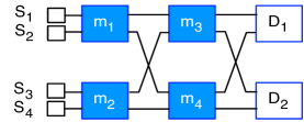
Refer to caption
Figure 10: The fictitious network for a 4×4444\times 4 Benes network.

Suppose the arrival rate vector is 𝒓=(rsd,s,d)Λ2={𝒓|s=14rsd1,d=14rsd1,s,d}𝒓subscript𝑟𝑠𝑑for-all𝑠𝑑subscriptΛ2conditional-set𝒓formulae-sequencesuperscriptsubscript𝑠14subscript𝑟𝑠𝑑1superscriptsubscript𝑑14subscript𝑟𝑠𝑑1for-all𝑠𝑑{\boldsymbol{r}}=(r_{sd},\,\forall\,s,d)\in\Lambda_{2}=\{{\boldsymbol{r}}\,|\,\sum_{s=1}^{4}r_{sd}\leq 1,\,\sum_{d=1}^{4}r_{sd}\leq 1,\,\,\forall\,s,d\}. We construct a stabilizing rate allocation profile 𝝁(𝒓)𝝁𝒓{\boldsymbol{\mu}}({\boldsymbol{r}}) as follows:

μsim1U=d=1,2rsid,μsim1L=d=3,4rsid,si=1,2,formulae-sequencesuperscriptsubscript𝜇subscript𝑠𝑖subscript𝑚1Usubscript𝑑12subscript𝑟subscript𝑠𝑖𝑑formulae-sequencesuperscriptsubscript𝜇subscript𝑠𝑖subscript𝑚1Lsubscript𝑑34subscript𝑟subscript𝑠𝑖𝑑for-allsubscript𝑠𝑖12\displaystyle\mu_{s_{i}m_{1}}^{\textsf{U}}=\sum_{d=1,2}r_{s_{i}d},\,\mu_{s_{i}m_{1}}^{\textsf{L}}=\sum_{d=3,4}r_{s_{i}d},\,\,\forall\,s_{i}=1,2,
μsim2U=d=1,2rsid,μsim2L=d=3,4rsid,si=3,4,formulae-sequencesuperscriptsubscript𝜇subscript𝑠𝑖subscript𝑚2Usubscript𝑑12subscript𝑟subscript𝑠𝑖𝑑formulae-sequencesuperscriptsubscript𝜇subscript𝑠𝑖subscript𝑚2Lsubscript𝑑34subscript𝑟subscript𝑠𝑖𝑑for-allsubscript𝑠𝑖34\displaystyle\mu_{s_{i}m_{2}}^{\textsf{U}}=\sum_{d=1,2}r_{s_{i}d},\,\mu_{s_{i}m_{2}}^{\textsf{L}}=\sum_{d=3,4}r_{s_{i}d},\,\,\forall\,s_{i}=3,4,
μm1,m3U=μm1,m4U=12d=1,2(r1d+r2d),superscriptsubscript𝜇subscript𝑚1subscript𝑚3Usuperscriptsubscript𝜇subscript𝑚1subscript𝑚4U12subscript𝑑12subscript𝑟1𝑑subscript𝑟2𝑑\displaystyle\mu_{m_{1},m_{3}}^{\textsf{U}}=\mu_{m_{1},m_{4}}^{\textsf{U}}=\frac{1}{2}\sum_{d=1,2}(r_{1d}+r_{2d}),
μm1,m3L=μm1,m4L=12d=3,4(r1d+r2d),superscriptsubscript𝜇subscript𝑚1subscript𝑚3Lsuperscriptsubscript𝜇subscript𝑚1subscript𝑚4L12subscript𝑑34subscript𝑟1𝑑subscript𝑟2𝑑\displaystyle\mu_{m_{1},m_{3}}^{\textsf{L}}=\mu_{m_{1},m_{4}}^{\textsf{L}}=\frac{1}{2}\sum_{d=3,4}(r_{1d}+r_{2d}),
μm2,m3U=μm2,m4U=12d=1,2(r3d+r4d),superscriptsubscript𝜇subscript𝑚2subscript𝑚3Usuperscriptsubscript𝜇subscript𝑚2subscript𝑚4U12subscript𝑑12subscript𝑟3𝑑subscript𝑟4𝑑\displaystyle\mu_{m_{2},m_{3}}^{\textsf{U}}=\mu_{m_{2},m_{4}}^{\textsf{U}}=\frac{1}{2}\sum_{d=1,2}(r_{3d}+r_{4d}),
μm2,m3L=μm2,m4L=12d=3,4(r3d+r4d),superscriptsubscript𝜇subscript𝑚2subscript𝑚3Lsuperscriptsubscript𝜇subscript𝑚2subscript𝑚4L12subscript𝑑34subscript𝑟3𝑑subscript𝑟4𝑑\displaystyle\mu_{m_{2},m_{3}}^{\textsf{L}}=\mu_{m_{2},m_{4}}^{\textsf{L}}=\frac{1}{2}\sum_{d=3,4}(r_{3d}+r_{4d}),
μm3,D1U=μm4,D1U=12d=1,2srsd,superscriptsubscript𝜇subscript𝑚3subscript𝐷1Usuperscriptsubscript𝜇subscript𝑚4subscript𝐷1U12subscript𝑑12subscript𝑠subscript𝑟𝑠𝑑\displaystyle\mu_{m_{3},D_{1}}^{\textsf{U}}=\mu_{m_{4},D_{1}}^{\textsf{U}}=\frac{1}{2}\sum_{d=1,2}\sum_{s}r_{sd},
μm3,D2L=μm4,D2L=12d=3,4srsd.superscriptsubscript𝜇subscript𝑚3subscript𝐷2Lsuperscriptsubscript𝜇subscript𝑚4subscript𝐷2L12subscript𝑑34subscript𝑠subscript𝑟𝑠𝑑\displaystyle\mu_{m_{3},D_{2}}^{\textsf{L}}=\mu_{m_{4},D_{2}}^{\textsf{L}}=\frac{1}{2}\sum_{d=3,4}\sum_{s}r_{sd}.

Since 𝒓Λ2𝒓subscriptΛ2{\boldsymbol{r}}\in\Lambda_{2}, it can be verified that 𝝁(𝒓)𝝁𝒓{\boldsymbol{\mu}}({\boldsymbol{r}}) satisfies all the constraints (41) - (44). Hence, it is a stabilizing rate allocation profile. This proves the 4×4444\times 4 case.

Now suppose the result holds for the 2n1×2n1superscript2𝑛1superscript2𝑛12^{n-1}\times 2^{n-1} Benes network, we show that it also holds for the 2n×2nsuperscript2𝑛superscript2𝑛2^{n}\times 2^{n} Benes network 𝔹nsubscript𝔹𝑛\mathbb{B}_{n}. To do so, let 𝒓Λn𝒓subscriptΛ𝑛{\boldsymbol{r}}\in\Lambda_{n} denote the input vector to 𝔹nsubscript𝔹𝑛\mathbb{B}_{n} and we construct a stabilizing rate allocation profile as follows.

First, for each input server s𝑠s, we let

μs,m(s)U=d2n1rsd,μs,m(s)L=d>2n1rsd.formulae-sequencesuperscriptsubscript𝜇𝑠𝑚𝑠Usubscript𝑑superscript2𝑛1subscript𝑟𝑠𝑑superscriptsubscript𝜇𝑠𝑚𝑠Lsubscript𝑑superscript2𝑛1subscript𝑟𝑠𝑑\displaystyle\mu_{s,m(s)}^{\textsf{U}}=\sum_{d\leq 2^{n-1}}r_{sd},\,\mu_{s,m(s)}^{\textsf{L}}=\sum_{d>2^{n-1}}r_{sd}. (74)

Then, for each m𝒞1𝑚subscript𝒞1m\in{{\cal{C}}}_{1}, we let:

μm,muU=μm,mlU=12s{2im1,2im}d2n1rsd,subscriptsuperscript𝜇U𝑚subscript𝑚𝑢subscriptsuperscript𝜇U𝑚subscript𝑚𝑙12subscript𝑠2subscript𝑖𝑚12subscript𝑖𝑚subscript𝑑superscript2𝑛1subscript𝑟𝑠𝑑\displaystyle\mu^{\textsf{U}}_{m,m_{u}}=\mu^{\textsf{U}}_{m,m_{l}}=\frac{1}{2}\sum_{s\in\{2i_{m}-1,2i_{m}\}}\sum_{d\leq 2^{n-1}}r_{sd}, (75)
μm,muL=μm,mlL=12s{2im1,2im}d>2n1rsd.subscriptsuperscript𝜇L𝑚subscript𝑚𝑢subscriptsuperscript𝜇L𝑚subscript𝑚𝑙12subscript𝑠2subscript𝑖𝑚12subscript𝑖𝑚subscript𝑑superscript2𝑛1subscript𝑟𝑠𝑑\displaystyle\mu^{\textsf{L}}_{m,m_{u}}=\mu^{\textsf{L}}_{m,m_{l}}=\frac{1}{2}\sum_{s\in\{2i_{m}-1,2i_{m}\}}\sum_{d>2^{n-1}}r_{sd}. (76)

Here s=2im1𝑠2subscript𝑖𝑚1s=2i_{m}-1 and 2im2subscript𝑖𝑚2i_{m} are the input servers that connect to m𝑚m. Note that (75) and (76) can also be viewed as equally splitting the traffic of each flow going through m𝒞1𝑚subscript𝒞1m\in{{\cal{C}}}_{1} to its two next-hop nodes musubscript𝑚𝑢m_{u} and mlsubscript𝑚𝑙m_{l}, one in the upper subnetwork and the other in the lower subnetwork. We thus take these as the traffic input rates to the two subnetworks of the Benes network.

Now consider the upper subnetwork and label all the input and output ports of the upper subnetwork by s{1,,2n1}superscript𝑠1superscript2𝑛1s^{\prime}\in\{1,...,2^{n-1}\} and d{1,,2n1}superscript𝑑1superscript2𝑛1d^{\prime}\in\{1,...,2^{n-1}\}. According to the construction rules of 𝔹nsubscript𝔹𝑛\mathbb{B}_{n} in Section III-A, an input port ssuperscript𝑠s^{\prime} is connected by the switch module in row ssuperscript𝑠s^{\prime} in 𝒞1subscript𝒞1{{\cal{C}}}_{1} of 𝔹nsubscript𝔹𝑛\mathbb{B}_{n}; while an outport dsuperscript𝑑d^{\prime} connects to the switch module in row dsuperscript𝑑d^{\prime} in 𝒞2n1subscript𝒞2𝑛1{{\cal{C}}}_{2n-1} of 𝔹nsubscript𝔹𝑛\mathbb{B}_{n}. These imply that the traffic going from input port ssuperscript𝑠s^{\prime} to output port dsuperscript𝑑d^{\prime} in the upper 2n1×2n1superscript2𝑛1superscript2𝑛12^{n-1}\times 2^{n-1} subnetwork indeed consists of the traffic going from input ports 2s12superscript𝑠12s^{\prime}-1 and 2s2superscript𝑠2s^{\prime} to 2d12superscript𝑑12d^{\prime}-1 and 2d2superscript𝑑2d^{\prime} in 𝔹nsubscript𝔹𝑛\mathbb{B}_{n}. Denote the rate of this traffic by r^sdsubscript^𝑟superscript𝑠superscript𝑑\hat{r}_{s^{\prime}d^{\prime}}. Using (75) and (76), we have:

r^sd=12[r(2s1)(2d1)+r(2s1)(2d)\displaystyle\hat{r}_{s^{\prime}d^{\prime}}=\frac{1}{2}\bigg{[}r_{(2s^{\prime}-1)(2d^{\prime}-1)}+r_{(2s^{\prime}-1)(2d^{\prime})} (77)
+r(2s)(2d1)+r(2s)(2d)].\displaystyle\qquad\qquad\qquad+r_{(2s^{\prime})(2d^{\prime}-1)}+r_{(2s^{\prime})(2d^{\prime})}\bigg{]}.

Hence, we have:

sr^sd=12s(rs(2d1)+rs(2d))1.subscriptsuperscript𝑠subscript^𝑟superscript𝑠superscript𝑑12subscript𝑠subscript𝑟𝑠2superscript𝑑1subscript𝑟𝑠2superscript𝑑1\displaystyle\sum_{s^{\prime}}\hat{r}_{s^{\prime}d^{\prime}}=\frac{1}{2}\sum_{s}(r_{s(2d^{\prime}-1)}+r_{s(2d^{\prime})})\leq 1. (78)

Similarly, we have:

dr^sd=12d(r(2s1)d+r(2s)d)1.subscriptsuperscript𝑑subscript^𝑟superscript𝑠superscript𝑑12subscript𝑑subscript𝑟2superscript𝑠1𝑑subscript𝑟2superscript𝑠𝑑1\displaystyle\sum_{d^{\prime}}\hat{r}_{s^{\prime}d^{\prime}}=\frac{1}{2}\sum_{d}(r_{(2s^{\prime}-1)d}+r_{(2s^{\prime})d})\leq 1. (79)

(78) and (79) thus imply that 𝒓^Λn1^𝒓subscriptΛ𝑛1\hat{{\boldsymbol{r}}}\in\Lambda_{n-1}. Hence, by induction, there exists a stabilizing rate allocation 𝝁^up(𝒓^)=(μm,mU,up,μm,mL,up,m,m)superscript^𝝁up^𝒓superscriptsubscript𝜇𝑚superscript𝑚Uupsuperscriptsubscript𝜇𝑚superscript𝑚Lupfor-all𝑚superscript𝑚\hat{{\boldsymbol{\mu}}}^{\text{up}}(\hat{{\boldsymbol{r}}})=(\mu_{m,m^{\prime}}^{\textsf{U},\text{up}},\mu_{m,m^{\prime}}^{\textsf{L},\text{up}},\,\forall\,m,m^{\prime}) that serves the arrival rate vector 𝒓^^𝒓\hat{{\boldsymbol{r}}} within the upper 2n1×2n1superscript2𝑛1superscript2𝑛12^{n-1}\times 2^{n-1} subnetwork in a symmetric manner, i.e., satisfies (46). Similarly, one can show that there exists a balanced stabilizing rate allocation 𝝁^low(𝒓^)=(μm,mU,low,μm,mL,low,m,m)superscript^𝝁low^𝒓superscriptsubscript𝜇𝑚superscript𝑚Ulowsuperscriptsubscript𝜇𝑚superscript𝑚Llowfor-all𝑚superscript𝑚\hat{{\boldsymbol{\mu}}}^{\text{low}}(\hat{{\boldsymbol{r}}})=(\mu_{m,m^{\prime}}^{\textsf{U},\text{low}},\mu_{m,m^{\prime}}^{\textsf{L},\text{low}},\,\forall\,m,m^{\prime}) for the lower subnetwork.

Now a stabilizing rate allocation profile for 𝔹nsubscript𝔹𝑛\mathbb{B}_{n} can be constructed as follows:

  • For an input server s𝒮𝑠𝒮s\in{{\cal{S}}}, we use μs,m(s)Usuperscriptsubscript𝜇𝑠𝑚𝑠U\mu_{s,m(s)}^{\textsf{U}} and μs,m(s)Lsuperscriptsubscript𝜇𝑠𝑚𝑠L\mu_{s,m(s)}^{\textsf{L}} as in (74).

  • For a switch module m𝒞1𝑚subscript𝒞1m\in{{\cal{C}}}_{1}, we use μm,muUsubscriptsuperscript𝜇U𝑚subscript𝑚𝑢\mu^{\textsf{U}}_{m,m_{u}}, μm,mlUsubscriptsuperscript𝜇U𝑚subscript𝑚𝑙\mu^{\textsf{U}}_{m,m_{l}}, μm,muLsubscriptsuperscript𝜇L𝑚subscript𝑚𝑢\mu^{\textsf{L}}_{m,m_{u}}, and μm,mlLsubscriptsuperscript𝜇L𝑚subscript𝑚𝑙\mu^{\textsf{L}}_{m,m_{l}} as in (75) and (76).

  • For the switch modules in the upper subnetwork, use 𝝁^up(𝒓^)superscript^𝝁up^𝒓\hat{{\boldsymbol{\mu}}}^{\text{up}}(\hat{{\boldsymbol{r}}}); for the switch modules in the lower subnetwork, use 𝝁^low(𝒓^)superscript^𝝁low^𝒓\hat{{\boldsymbol{\mu}}}^{\text{low}}(\hat{{\boldsymbol{r}}}).

It can be verified that this rate vector satisfies all the constraints (41) - (44), and thus is a stabilizing rate allocation vector for 𝔹nsubscript𝔹𝑛\mathbb{B}_{n}. By induction, this proves the theorem. ∎

References

  • [1] A. Singla, C. Hong, L. Popa, and P. B. Godfrey. Jellyfish: Networking data centers randomly. Proceedings of NSDI, 2012.
  • [2] A. Greenberg, J. R. Hamilton, N. Jain, S. Kandula, C. Kim, P. Lahiri, D. A. Maltz nd P. Patel, and S. Sengupta. Vl2: A scalable and flexible data center network. Proceedings of SIGCOMM, 2009.
  • [3] C. Guo, H. Wu, K.Tan, L. Shi, Y. Zhang, and S. Lu. Dcell: A scalable and fault-tolerant network structure for data centers. Proceedings of SIGCOMM, 2008.
  • [4] L. Gyarmati and T. Anh Trinh. Scafida: A scale-free network inspired data center architecture. Proceedings of SIGCOMM, 2010.
  • [5] M. Al-Fares, A. Loukissas, and A. Vahdat. A scalable commodity data center network architecture. Proceedings of SIGCOMM, 2008.
  • [6] P. Costa, A. Donnelly, A. Rowstron, and G. O Shea. Camdoop: Exploiting in-network aggregation for big data applications. Proceedings of NSDI, 2012.
  • [7] G. Wang, D. G. Andersen, M. Kaminsky, K. Papagiannaki, T. S. E. Ng, M. Kozuch, and M. Ryan. c-through: Part-time optics in data centers. Proceedings of SIGCOMM, 2010.
  • [8] V. E. Benesˇˇ𝑠\check{s}. Permutation groups, complexes and rearrangeable connecting network. Bell System Technical Journal, 43, 4:1619 1640, 1964.
  • [9] V. E. Benesˇˇ𝑠\check{s}. Mathematical theory of connecting networks and telephone traffic. Academic Press Inc., New Yrok, 1965.
  • [10] F. Kelly. Charging and rate control for elastic traffic. European Transactions on Telecommunications, vol. 8, pp. 33-37, 1997.
  • [11] M. Chiang, S. H. Low, A. R. Calderbank, and J. C. Doyle. Layering as optimization decomposition: A mathematical theory of network architectures. Proceedings of the IEEE, Vol. 95, No. 1, January 2007.
  • [12] L. Georgiadis, M. J. Neely, and L. Tassiulas. Resource Allocation and Cross-Layer Control in Wireless Networks. Foundations and Trends in Networking Vol. 1, no. 1, pp. 1-144, 2006.
  • [13] M. J. Neely, E. Modiano, and C. Li. Fairness and optimal stochastic control for heterogeneous networks. IEEE/ACM Trans. on Networking, vol. 16, no. 2, pp. 396-409, April 2008.
  • [14] L. Ying, R. Srikant, and D. Towsley. Cluster-based back-pressure routing algorithm. Proc. of IEEE INFOCOM, April 2008.
  • [15] L. Bui, R. Srikant, and A. Stolyar. Novel architectures and algorithms for delay reduction in back-pressure scheduling and routing. Proceedings of IEEE INFOCOM 2009 Mini-Conference, April 2009.
  • [16] M. J. Neely, E. Modiano, and C. E. Rohrs. Dynamic power allocation and routing for time-varying wireless networks. IEEE Journal on Selected Areas in Communications, Vol 23, NO.1, pp. 89-103, January 2005.