Mixed perturbations from an Inflaton and Two Curvatons - towards understanding non-gaussianity in more complicated curvaton scenarios

Maria Sueiro and Malcolm Fairbairn
Physics, King’s College London,
Strand, London WC2R 2LS, UK
(2nd August 2012)
Abstract

We analyse the situation where the primordial curvature perturbations are produced by the joint effects of an inflaton field and two curvaton fields. We present general equations which allow the reader to obtain fN​Lsubscript𝑓𝑁𝐿f_{NL} for several different scenarios which differ in the order in which fields decay into radiation after inflation. In order to investigate the physics of these equations we analyse some simplified situations where the fields are harmonic and both curvatons are frozen at the same expectation value during inflation. We find quite complex behaviour - for a given situation where the inflaton contributes a fixed amount to the total curvature perturbation there are situations where fN​Lsubscript𝑓𝑁𝐿f_{NL} is maximised if both curvatons share equally in contributing the rest and situations where fN​Lsubscript𝑓𝑁𝐿f_{NL} is maximised if only one of the two curvatons contributes the rest. We are unable therefore to make any completely general extrapolations about the expected non-gaussianity from N𝑁N curvatons. We find that as the curvaton contribution to the overall perturbation is gradually increased, fN​Lsubscript𝑓𝑁𝐿f_{NL} rises to a maximum before falling again and that a given fN​Lsubscript𝑓𝑁𝐿f_{NL} can correspond to many different parameter sets for the two curvatons.

1 Introduction

Inflation is the most successful theory we have to describe the early universe. According to inflation [1], at some early time the universe underwent an accelerated expansion, and this solves the horizon and flatness problem while also predicting an almost scale-invariant power spectrum in the cosmic microwave background, consistent with current observations. The most basic models of inflation (see, for example, [2]) involve a single, massive scalar field Ο•italic-Ο•\phi called the inflaton, which slowly rolls down its potential to source the necessary expansion. Once it reaches the minimum of the potential it oscillates around that point, reheating the Universe by decaying into standard model particles. The quantum fluctuations of the inflaton get stretched out with the expansion and become classical perturbations, causing inhomogeneities which upon horizon re-entry evolve to become the large-scale structure that we observe today [3].

Since many theories that go beyond the standard model predict scalar fields, it is not unreasonable to assume that in early times, these fields had expectation values away from the minimum of their potential. Such fields, known as curvaton fields, can be present during inflation but only begin to move when the Hubble parameter drops down to their mass (as in [4] and [5]). They then proceed to oscillate around the minimum of their potential and eventually decay when the Hubble parameter is equal to their decay rate. The presence of these particles imprints a record of the curvaton perturbations as well as the inflaton perturbations upon the cosmic distribution of matter and therefore provides a different mechanism for the creation of the primordial curvature perturbation ΢𝜁\zeta and can alter the predictions of basic single-field inflation [6], [7], [8], [9], [10]. There are a plethora of curvaton models one can imagine existing in particle physics and string theory and they typically include a large number of parameters. To constrain them, one needs to compare their predictions to current astrophysical observations, with the most popular discriminant being the non-gaussianity parameter, fN​Lsubscript𝑓𝑁𝐿f_{NL} ([11], [12],[13], [14]).

The idea behind the curvaton scenario is to boost small perturbations and make them larger by virtue of the energy density in the curvaton field red-shifting more slowly than the energy density from the inflaton field. This occurs once the inflaton has decayed into radiation but the curvaton is still oscillating (and thus red-shifting like matter). There are therefore multiple scenarios depending upon the order in which the inflaton decays, the curvaton starts to move and the curvaton decays. In this work we will attempt to study a number of these different situations, although we will not consider the case where the curvaton starts to roll during inflation, as this moves into the territory of multifield inflation.

In inflation models, the non-gaussianity parameter fN​Lsubscript𝑓𝑁𝐿f_{NL} is related to the curvature perturbation after the last decay. This parameter is a measure of deviations from a purely Gaussian distribution of the primordial curvature perturbation and the current fN​Lsubscript𝑓𝑁𝐿f_{NL} limits are given by WMAP 7 to be βˆ’10<fN​L<7410subscript𝑓𝑁𝐿74-10<f_{NL}<74 [15]. We analytically compute the expression for ΢𝜁\zeta at the last decay and fN​Lsubscript𝑓𝑁𝐿f_{NL} in models with one inflaton, Ο•italic-Ο•\phi, and two curvatons, ΟƒπœŽ\sigma and Ο‡πœ’\chi, for various sequences of particle decays. In each case, the inflaton is the one responsible for producing the necessary e-folds and both the curvatons are frozen during the inflaton’s slow-roll. Once inflation has finished, Ο•italic-Ο•\phi begins to oscillate around the minimum of its potential and then decays. Independently, some time after the end of inflation, when H=mc​u​r​v​a​t​o​n𝐻subscriptπ‘šπ‘π‘’π‘Ÿπ‘£π‘Žπ‘‘π‘œπ‘›H=m_{curvaton}, the curvatons begin to oscillate and eventually decay. All three particles contribute to the curvature perturbation. We will evaluate the primordial curvature perturbation at the time of the last particle’s decay, whether it is the inflaton or one of the curvatons.

2 Perturbations and Non-Gaussianity with multiple fields

In this section we will present our notation and derive some general expressions for the curvature perturbation ΢𝜁\zeta and the non-gaussianity parameter fN​Lsubscript𝑓𝑁𝐿f_{NL} which we will be able to use in the following sections.

2.1 Curvature perturbation from the curvatons

The simplest potential used in inflationary models is the quadratic, V=12​mΟ•2​ϕ2𝑉12superscriptsubscriptπ‘šitalic-Ο•2superscriptitalic-Ο•2V=\frac{1}{2}m_{\phi}^{2}\phi^{2} which we will use later on for our examples but in our equations we are allowing the curvaton potential to deviate from this case away from its minimum.

For each of the two curvatons, the oscillation amplitude will then be a function of the initial field expectation value at horizon exit, i.e. Οƒ=c​(Οƒβˆ—)πœŽπ‘subscript𝜎\sigma=c(\sigma_{*}) and Ο‡=d​(Ο‡βˆ—)πœ’π‘‘subscriptπœ’\chi=d(\chi_{*}) respectively where the index βˆ—* means the expectation value at horizon exit. This general case simplifies to the quadratic potential when c=Οƒβˆ—β‡’cβ€²=1𝑐subscriptπœŽβ‡’superscript𝑐′1c=\sigma_{*}\Rightarrow c^{\prime}=1 and d=Ο‡βˆ—β‡’dβ€²=1𝑑subscriptπœ’β‡’superscript𝑑′1d=\chi_{*}\Rightarrow d^{\prime}=1. The curvature perturbation up to second order for ΟƒπœŽ\sigma is derived in [19] and it is

ΞΆΟƒ(1)subscriptsubscript𝜁𝜎1\displaystyle{\zeta_{\sigma}}_{(1)} =\displaystyle= 23​δ​σσ¯,23π›ΏπœŽΒ―πœŽ\displaystyle\frac{2}{3}\frac{\delta\sigma}{\bar{\sigma}}, (1)
ΞΆΟƒ(2)subscriptsubscript𝜁𝜎2\displaystyle{\zeta_{\sigma}}_{(2)} =\displaystyle= βˆ’32​(1βˆ’c​cβ€²β€²c′⁣2)​΢σ(1)2321𝑐superscript𝑐′′superscript𝑐′2superscriptsubscriptsubscript𝜁𝜎12\displaystyle-\frac{3}{2}\left(1-\frac{cc^{\prime\prime}}{c^{\prime 2}}\right){\zeta_{\sigma}}_{(1)}^{2} (2)

the expressions for the other curvaton, Ο‡πœ’\chi will take a similar form. For each case that we study we will use ΞΆΟ•subscript𝜁italic-Ο•\zeta_{\phi}, ΞΆΟƒsubscript𝜁𝜎\zeta_{\sigma} and ΞΆΟ‡subscriptπœπœ’\zeta_{\chi} to define the isocurvature perturbation, Si∝΢iβˆ’ΞΆΟ•proportional-tosubscript𝑆𝑖subscriptπœπ‘–subscript𝜁italic-Ο•S_{i}\propto\zeta_{i}-\zeta_{\phi}, i=Οƒ,Ο‡π‘–πœŽπœ’i=\sigma,\chi, to describe the non-adiabatic part of the curvature perturbation of the curvatons. Next, we define the general curvature perturbation in terms of ΞΆΟ•subscript𝜁italic-Ο•\zeta_{\phi}, SΟƒsubscriptπ‘†πœŽS_{\sigma} and SΟ‡subscriptπ‘†πœ’S_{\chi} to look at the non-gaussianity parameter fN​Lsubscript𝑓𝑁𝐿f_{NL}.

2.2 General expression for fN​Lsubscript𝑓𝑁𝐿f_{NL}

In this section, following a similar formalism as in [16], we derive the general expression for the fN​Lsubscript𝑓𝑁𝐿f_{NL} parameter in terms of the coefficients in the curvature perturbation produced in a model with one inflaton and two curvatons, taking into account contributions from all three particles.

Up to second order, the general form of the primordial curvature perturbation will be:

΢𝜁\displaystyle\zeta =\displaystyle= A​΢ϕ(1)+B​SΟƒ(1)+Γ​SΟ‡(1)Asubscriptsubscript𝜁italic-Ο•1Bsubscriptsubscriptπ‘†πœŽ1Ξ“subscriptsubscriptπ‘†πœ’1\displaystyle{\rm A}{\zeta_{\phi}}_{(1)}+{\rm B}{S_{\sigma}}_{(1)}+\Gamma{S_{\chi}}_{(1)} (3)
+12​Δ​΢ϕ(1)2+12​E​SΟƒ(1)2+12​Z​SΟ‡(1)212Ξ”superscriptsubscriptsubscript𝜁italic-Ο•1212Esuperscriptsubscriptsubscriptπ‘†πœŽ1212Zsuperscriptsubscriptsubscriptπ‘†πœ’12\displaystyle+\frac{1}{2}\Delta{\zeta_{\phi}}_{(1)}^{2}+\frac{1}{2}{\rm E}{S_{\sigma}}_{(1)}^{2}+\frac{1}{2}{\rm Z}{S_{\chi}}_{(1)}^{2}
+12​H​΢ϕ(1)​SΟƒ(1)+12β€‹Ξ˜β€‹ΞΆΟ•(1)​SΟ‡(1)+12​I​SΟƒ(1)​SΟ‡(1)12Hsubscriptsubscript𝜁italic-Ο•1subscriptsubscriptπ‘†πœŽ112Θsubscriptsubscript𝜁italic-Ο•1subscriptsubscriptπ‘†πœ’112Isubscriptsubscriptπ‘†πœŽ1subscriptsubscriptπ‘†πœ’1\displaystyle+\frac{1}{2}{\rm H}{\zeta_{\phi}}_{(1)}{S_{\sigma}}_{(1)}+\frac{1}{2}\Theta{\zeta_{\phi}}_{(1)}{S_{\chi}}_{(1)}+\frac{1}{2}{\rm I}{S_{\sigma}}_{(1)}{S_{\chi}}_{(1)}

evaluated at the time of the last decay (the point at which all three fields have decayed into radiation). Since fN​Lsubscript𝑓𝑁𝐿f_{NL} is related to the primordial bi-spectrum, we compute the three point correlator of the curvature perturbation:

βŸ¨ΞΆβ€‹(𝐀1)​΢​(𝐀2)​΢​(𝐀3)⟩delimited-⟨⟩𝜁subscript𝐀1𝜁subscript𝐀2𝜁subscript𝐀3\displaystyle\langle\zeta(\mathbf{k}_{1})\zeta(\mathbf{k}_{2})\zeta(\mathbf{k}_{3})\rangle =\displaystyle= {[A2Ξ”P΢ϕ​1(k1)P΢ϕ​1(k2)+B2EPSσ​1(k1)PSσ​1(k2)\displaystyle\{[{\rm A}^{2}\Delta P_{\zeta_{\phi 1}}(k_{1})P_{\zeta_{\phi 1}}(k_{2})+{\rm B^{2}E}P_{S_{\sigma 1}}(k_{1})P_{S_{\sigma 1}}(k_{2}) (4)
+Ξ“2​Z​PSχ​1​(k1)​PSχ​1​(k2)+12​ABH​P΢ϕ​1​(k1)​PSσ​1​(k2)superscriptΞ“2Zsubscript𝑃subscriptπ‘†πœ’1subscriptπ‘˜1subscript𝑃subscriptπ‘†πœ’1subscriptπ‘˜212ABHsubscript𝑃subscript𝜁italic-Ο•1subscriptπ‘˜1subscript𝑃subscriptπ‘†πœŽ1subscriptπ‘˜2\displaystyle+\Gamma^{2}{\rm Z}P_{S_{\chi 1}}(k_{1})P_{S_{\chi 1}}(k_{2})+\frac{1}{2}{\rm ABH}P_{\zeta_{\phi 1}}(k_{1})P_{S_{\sigma 1}}(k_{2})
+12AΞ“Ξ˜P΢ϕ​1(k1)PSχ​1(k2)+12BΞ“IPSσ​1(k1)PSχ​1(k2)]\displaystyle+\frac{1}{2}{\rm A}\Gamma\Theta P_{\zeta_{\phi 1}}(k_{1})P_{S_{\chi 1}}(k_{2})+\frac{1}{2}{\rm B}\Gamma{\rm I}P_{S_{\sigma 1}}(k_{1})P_{S_{\chi 1}}(k_{2})]
+permutations}(2Ο€)3Ξ΄(3)(𝐀𝟏+𝐀𝟐+π€πŸ‘)\displaystyle+\textrm{permutations}\}(2\pi)^{3}\delta^{(3)}(\mathbf{k_{1}}+\mathbf{k_{2}}+\mathbf{k_{3}})

where we have assumed that the adiabatic perturbation is uncorrelated with the isocurvature perturbations, so βŸ¨ΞΆΟ•(1)​(𝐀𝟏)​SΟƒ(1)​(𝐀𝟐)⟩=βŸ¨ΞΆΟ•(1)​(𝐀𝟏)​SΟ‡(1)​(𝐀𝟐)⟩=⟨SΟƒ(1)​(𝐀𝟏)​SΟ‡(1)​(𝐀𝟐)⟩=0delimited-⟨⟩subscript𝜁subscriptitalic-Ο•1subscript𝐀1subscript𝑆subscript𝜎1subscript𝐀2delimited-⟨⟩subscript𝜁subscriptitalic-Ο•1subscript𝐀1subscript𝑆subscriptπœ’1subscript𝐀2delimited-⟨⟩subscript𝑆subscript𝜎1subscript𝐀1subscript𝑆subscriptπœ’1subscript𝐀20\langle\zeta_{\phi_{(1)}}(\mathbf{k_{1}})S_{\sigma_{(1)}}(\mathbf{k_{2}})\rangle=\langle\zeta_{\phi_{(1)}}(\mathbf{k_{1}})S_{\chi_{(1)}}(\mathbf{k_{2}})\rangle=\langle S_{\sigma_{(1)}}(\mathbf{k_{1}})S_{\chi_{(1)}}(\mathbf{k_{2}})\rangle=0. By looking at equation (3), we can now see that the power spectrum for ΢𝜁\zeta at leading order is just given by

PΞΆ=A2​PΞΆΟ•+B2​PSΟƒ+Ξ“2​PSΟ‡subscriptπ‘ƒπœsuperscriptA2subscript𝑃subscript𝜁italic-Ο•superscriptB2subscript𝑃subscriptπ‘†πœŽsuperscriptΞ“2subscript𝑃subscriptπ‘†πœ’P_{\zeta}={\rm A}^{2}P_{\zeta_{\phi}}+{\rm B}^{2}P_{S_{\sigma}}+\Gamma^{2}P_{S_{\chi}} (5)

Where the power spectrum for each component is [16],[17], [10]:

PΞΆΟ•subscript𝑃subscript𝜁italic-Ο•\displaystyle P_{\zeta_{\phi}} =\displaystyle= 12​MP​l2β€‹Ο΅βˆ—β€‹(Hβˆ—2​π)212superscriptsubscript𝑀𝑃𝑙2subscriptitalic-Ο΅superscriptsubscript𝐻2πœ‹2\displaystyle\frac{1}{2M_{Pl}^{2}\epsilon_{*}}\left(\frac{H_{*}}{2\pi}\right)^{2} (6)
PSΟƒsubscript𝑃subscriptπ‘†πœŽ\displaystyle P_{S_{\sigma}} =\displaystyle= 4​(cβ€²c)2​(Hβˆ—2​π)24superscriptsuperscript𝑐′𝑐2superscriptsubscript𝐻2πœ‹2\displaystyle 4\left(\frac{c^{\prime}}{c}\right)^{2}\left(\frac{H_{*}}{2\pi}\right)^{2} (7)
PSΟ‡subscript𝑃subscriptπ‘†πœ’\displaystyle P_{S_{\chi}} =\displaystyle= 4​(dβ€²d)2​(Hβˆ—2​π)24superscriptsuperscript𝑑′𝑑2superscriptsubscript𝐻2πœ‹2\displaystyle 4\left(\frac{d^{\prime}}{d}\right)^{2}\left(\frac{H_{*}}{2\pi}\right)^{2} (8)

here Ο΅βˆ—subscriptitalic-Ο΅\epsilon_{*} is the inflaton slow-roll parameter and MP​lsubscript𝑀𝑃𝑙M_{Pl} is the reduced Planck mass, MP​l=(8​π​G)βˆ’1/2subscript𝑀𝑃𝑙superscript8πœ‹πΊ12M_{Pl}=(8\pi G)^{-1/2}.

Combining equations (5),(6), (7) and (8) we can express all three individual components of the power spectrum PΞΆΟ•subscript𝑃subscript𝜁italic-Ο•P_{\zeta_{\phi}}, PSΟƒsubscript𝑃subscriptπ‘†πœŽP_{S_{\sigma}} and PSΟ‡subscript𝑃subscriptπ‘†πœ’P_{S_{\chi}} in terms of the total PΞΆsubscriptπ‘ƒπœP_{\zeta}, and thus substitute them in the bi-spectrum equation (4). The non-linearity parameter is defined in the following way:

βŸ¨ΞΆβ€‹(𝐀1)​΢​(𝐀2)​΢​(𝐀3)⟩delimited-⟨⟩𝜁subscript𝐀1𝜁subscript𝐀2𝜁subscript𝐀3\displaystyle\langle\zeta(\mathbf{k}_{1})\zeta(\mathbf{k}_{2})\zeta(\mathbf{k}_{3})\rangle =\displaystyle= B​(k1,k2,k3)​(2​π)3​δ(3)​(𝐀𝟏+𝐀𝟐+π€πŸ‘)𝐡subscriptπ‘˜1subscriptπ‘˜2subscriptπ‘˜3superscript2πœ‹3superscript𝛿3subscript𝐀1subscript𝐀2subscript𝐀3\displaystyle B(k_{1},k_{2},k_{3})(2\pi)^{3}\delta^{(3)}(\mathbf{k_{1}}+\mathbf{k_{2}}+\mathbf{k_{3}})
B​(k1,k2,k3)𝐡subscriptπ‘˜1subscriptπ‘˜2subscriptπ‘˜3\displaystyle B(k_{1},k_{2},k_{3}) =\displaystyle= 65​fN​L​[P΢​(k1)​P΢​(k2)+permutations].65subscript𝑓𝑁𝐿delimited-[]subscriptπ‘ƒπœsubscriptπ‘˜1subscriptπ‘ƒπœsubscriptπ‘˜2permutations\displaystyle\frac{6}{5}f_{NL}[P_{\zeta}(k_{1})P_{\zeta}(k_{2})+\textrm{permutations}].

And so we are able to obtain the following equation for the fN​Lsubscript𝑓𝑁𝐿f_{NL} parameter:

fN​Lsubscript𝑓𝑁𝐿\displaystyle f_{NL} =\displaystyle= 561[A2​c2​d2+8​B2​MP​l2β€‹Ο΅βˆ—β€‹c′⁣2​d2+8​Γ2​MP​l2β€‹Ο΅βˆ—β€‹c2​d′⁣2]2Γ—{A2Ξ”c4d4\displaystyle\frac{5}{6}\frac{1}{[{\rm A}^{2}c^{2}d^{2}+8{\rm B}^{2}M_{Pl}^{2}\epsilon_{*}c^{\prime 2}d^{2}+8\Gamma^{2}M_{Pl}^{2}\epsilon_{*}c^{2}d^{\prime 2}]^{2}}\times\{{\rm A}^{2}\Delta c^{4}d^{4} (9)
+64​B2​E​MP​l4β€‹Ο΅βˆ—2​c′⁣4​d4+64​Γ2​Z​MP​l4β€‹Ο΅βˆ—2​c4​d′⁣4+4​A​B​H​MP​l2β€‹Ο΅βˆ—β€‹c2​c′⁣2​d464superscriptB2Esuperscriptsubscript𝑀𝑃𝑙4superscriptsubscriptitalic-Ο΅2superscript𝑐′4superscript𝑑464superscriptΞ“2Zsuperscriptsubscript𝑀𝑃𝑙4superscriptsubscriptitalic-Ο΅2superscript𝑐4superscript𝑑′44ABHsuperscriptsubscript𝑀𝑃𝑙2subscriptitalic-Ο΅superscript𝑐2superscript𝑐′2superscript𝑑4\displaystyle+64{\rm B}^{2}{\rm E}M_{Pl}^{4}\epsilon_{*}^{2}c^{\prime 4}d^{4}+64\Gamma^{2}{\rm Z}M_{Pl}^{4}\epsilon_{*}^{2}c^{4}d^{\prime 4}+4{\rm ABH}M_{Pl}^{2}\epsilon_{*}c^{2}c^{\prime 2}d^{4}
+4AΞ“Ξ˜MP​l2Ο΅βˆ—c4d2d′⁣2+32BΞ“IMP​l4Ο΅βˆ—2c2c′⁣2d2d′⁣2}\displaystyle+4{\rm A}\Gamma\Theta M_{Pl}^{2}\epsilon_{*}c^{4}d^{2}d^{\prime 2}+32{\rm B}\Gamma{\rm I}M_{Pl}^{4}\epsilon_{*}^{2}c^{2}c^{\prime 2}d^{2}d^{\prime 2}\}

This complicated looking expression is the general form of the non-linearity parameter when one inflaton and two curvatons are all contributing to the total curvature perturbation. The particular values of the parameters A,B,Γ𝐴𝐡ΓA,B,\Gamma etc. depend upon the particular cosmic history. In the following sections we analytically compute the coefficients A,B,Ξ“,…ABΓ…{\rm A,B},\Gamma,... for several different cases. However before we do that we will check for consistency with previous results.

2.2.1 First Consistency Check - fN​Lsubscript𝑓𝑁𝐿f_{NL} for curvatons without perturbations from inflation.

Before looking at the relatively complicated situation of mixed perturbations from an inflaton and two curvatons, we would like to check that our general equation (9) is able to re-create the results of others in particular limits. The first such consistency check, i.e. the case where the perturbations come from two curvatons with no contribution from inflation, can be done immediately. The other two consistency checks we will make (expression for a single curvaton and mixed perturbations from one inflaton and one curvaton) will have to wait until the parameters A,B,Ξ“,ΔΓΔ\Gamma,\Delta… etc have been defined in the next section.

If in our analysis above, we assume that the inflaton’s contribution to the primordial curvature perturbation can be ignored, we have the case where the perturbations are coming from two curvatons alone. In this case, A=Ξ”=H=Θ=0AΞ”HΘ0{\rm A}={\Delta}={\rm H}=\Theta=0 and it is straightforward to see that the expression for fN​Lsubscript𝑓𝑁𝐿f_{NL} becomes

fN​L=56​B2​E+12​λ2​B​Γ​I+Ξ»4​Γ2​Z(B2+Ξ»2​Γ2)2subscript𝑓𝑁𝐿56superscriptB2E12superscriptπœ†2BΞ“Isuperscriptπœ†4superscriptΞ“2ZsuperscriptsuperscriptB2superscriptπœ†2superscriptΞ“22f_{NL}=\frac{5}{6}\frac{{\rm B}^{2}{\rm E}+\frac{1}{2}\lambda^{2}{\rm B}\Gamma{\rm I}+\lambda^{4}\Gamma^{2}{\rm Z}}{({\rm B}^{2}+\lambda^{2}\Gamma^{2})^{2}} (10)

where Ξ»=Οƒβˆ—/Ο‡βˆ—πœ†subscript𝜎subscriptπœ’\lambda=\sigma_{*}/\chi_{*}. We have also assumed linear evolution of the two curvaton fields since horizon exit and so c=Οƒβˆ—π‘subscript𝜎c=\sigma_{*} and d=Ο‡βˆ—π‘‘subscriptπœ’d=\chi_{*}. This is in agreement with the expression derived in [16] for this particular case.

3 Mixed perturbations from an inflaton and two curvatons

Now we move on to the main part of the analysis in this paper, namely the situation where the efolds of inflation required to solve the horizon problem are achieved through the stress energy of a single field, while the primordial perturbations are made up out of the individual curvature perturbations of all three fields.

We will calculate the primordial curvature perturbation after all the particles have decayed using the δ​N𝛿𝑁\delta N formalism and the sudden decay approximation (for a different approach, using the ADM formalism see, [18]). This means that we assume that as soon as the Hubble parameter H𝐻H, becomes equal to the decay rate Ξ“isubscriptΓ𝑖\Gamma_{i} of a particle, the particle decays instantly and transfers all of its energy density (and curvature perturbation) into radiation. In our study we will follow the formalism of [19] and [16]: we will obtain a chain of four equations to describe the evolution of our model starting from a time when just one particle has decayed through to the last particle’s decay. Our goal is to find the first and second order components of the curvature perturbation at the last decay, expressed in terms of the initial adiabatic and isocurvature perturbations: ΞΆΟ•subscript𝜁italic-Ο•\zeta_{\phi}, SΟƒsubscriptπ‘†πœŽS_{\sigma} and SΟ‡subscriptπ‘†πœ’S_{\chi}. However, we generalise this method to include the linear terms coming from the inflaton, and up to second order terms from the two curvatons. Also, different orders of decay for the three particles will be considered, as well as situations where one of the curvatons is frozen until after the other two particles have decayed. Once we have the expression for ΢𝜁\zeta, we can manipulate it in the general form of (3) to find the coefficients we need to evaluate fN​Lsubscript𝑓𝑁𝐿f_{NL}.

3.1 Case 1: tΟƒo​s​c<tΟ‡o​s​c<tΟ•d​e​c​a​y<tΟƒd​e​c​a​y<tΟ‡d​e​c​a​ysubscript𝑑subscriptπœŽπ‘œπ‘ π‘subscript𝑑subscriptπœ’π‘œπ‘ π‘subscript𝑑subscriptitalic-Ο•π‘‘π‘’π‘π‘Žπ‘¦subscript𝑑subscriptπœŽπ‘‘π‘’π‘π‘Žπ‘¦subscript𝑑subscriptπœ’π‘‘π‘’π‘π‘Žπ‘¦t_{\sigma_{osc}}<t_{\chi_{osc}}<t_{\phi_{decay}}<t_{\sigma_{decay}}<t_{\chi_{decay}}

In this case, the two curvatons begin oscillating some time after the end of inflation, but decay after the inflaton has decayed. We are assuming that the energy density of each particle becomes radiation with the particle’s decay. When a particle is oscillating, its equation of state is the one for pressure-less matter, p=0𝑝0p=0, while for a radiation component it is p=13​ρ𝑝13𝜌p=\frac{1}{3}\rho. So, after the inflaton decay but before the first curvaton decay (in other words, while the two curvatons are oscillating) the curvature perturbation and energy density of each species is

ΞΆΟ•subscript𝜁italic-Ο•\displaystyle\zeta_{\phi} =\displaystyle= ΞΆΞ±+14​ln⁑(ρϕαρ¯ϕα)⇒ρϕα=ρ¯ϕα​e4​(ΞΆΟ•βˆ’ΞΆΞ±)β‡’subscriptπœπ›Ό14subscript𝜌subscriptitalic-ϕ𝛼subscript¯𝜌subscriptitalic-ϕ𝛼subscript𝜌subscriptitalic-ϕ𝛼subscript¯𝜌subscriptitalic-ϕ𝛼superscripte4subscript𝜁italic-Ο•subscriptπœπ›Ό\displaystyle\zeta_{\alpha}+\frac{1}{4}\ln(\frac{\rho_{\phi_{\alpha}}}{\bar{\rho}_{\phi_{\alpha}}})\Rightarrow\rho_{\phi_{\alpha}}=\bar{\rho}_{\phi_{\alpha}}\rm e^{4(\zeta_{\phi}-\zeta_{\alpha})} (11)
ΞΆΟƒsubscript𝜁𝜎\displaystyle\zeta_{\sigma} =\displaystyle= ΞΆΞ±+13​ln⁑(ρσαρ¯σα)⇒ρσα=ρ¯σα​e3​(ΞΆΟƒβˆ’ΞΆΞ±)β‡’subscriptπœπ›Ό13subscript𝜌subscriptπœŽπ›Όsubscript¯𝜌subscriptπœŽπ›Όsubscript𝜌subscriptπœŽπ›Όsubscript¯𝜌subscriptπœŽπ›Όsuperscripte3subscript𝜁𝜎subscriptπœπ›Ό\displaystyle\zeta_{\alpha}+\frac{1}{3}\ln(\frac{\rho_{\sigma_{\alpha}}}{\bar{\rho}_{\sigma_{\alpha}}})\Rightarrow\rho_{\sigma_{\alpha}}=\bar{\rho}_{\sigma_{\alpha}}\rm e^{3(\zeta_{\sigma}-\zeta_{\alpha})} (12)
ΞΆΟ‡subscriptπœπœ’\displaystyle\zeta_{\chi} =\displaystyle= ΞΆΞ±+13​ln⁑(ρχαρ¯χα)⇒ρχα=ρ¯χα​e3​(ΞΆΟ‡βˆ’ΞΆΞ±).β‡’subscriptπœπ›Ό13subscript𝜌subscriptπœ’π›Όsubscript¯𝜌subscriptπœ’π›Όsubscript𝜌subscriptπœ’π›Όsubscript¯𝜌subscriptπœ’π›Όsuperscripte3subscriptπœπœ’subscriptπœπ›Ό\displaystyle\zeta_{\alpha}+\frac{1}{3}\ln(\frac{\rho_{\chi_{\alpha}}}{\bar{\rho}_{\chi_{\alpha}}})\Rightarrow\rho_{\chi_{\alpha}}=\bar{\rho}_{\chi_{\alpha}}\rm e^{3(\zeta_{\chi}-\zeta_{\alpha})}. (13)

The index α𝛼\alpha symbolises the time at which the first curvaton decays and we will use β𝛽\beta to denote the time at which the second curvaton decays, which will be the last decay of the three fields in all the scenarios analysed in this paper. In the equations above, ΞΆΞ±subscriptπœπ›Ό\zeta_{\alpha} is the total curvature perturbation at the first curvaton decay and ρ¯isubscriptΒ―πœŒπ‘–\bar{\rho}_{i} is the average energy density of each field i𝑖i. We can assume that at this point the total curvature perturbation is equal to the adiabatic perturbation and so equations (12) and (13) become

ρσα=ρ¯σα​eSΟƒ,Sσ≑3​(ΞΆΟƒβˆ’ΞΆΟ•)formulae-sequencesubscript𝜌subscriptπœŽπ›Όsubscript¯𝜌subscriptπœŽπ›ΌsuperscriptesubscriptS𝜎subscriptS𝜎3subscript𝜁𝜎subscript𝜁italic-Ο•\displaystyle\rho_{\sigma_{\alpha}}=\bar{\rho}_{\sigma_{\alpha}}\rm e^{S_{\sigma}},S_{\sigma}\equiv 3(\zeta_{\sigma}-\zeta_{\phi}) (14)
ρχα=ρ¯χα​eSΟ‡,Sχ≑3​(ΞΆΟ‡βˆ’ΞΆΟ•).formulae-sequencesubscript𝜌subscriptπœ’π›Όsubscript¯𝜌subscriptπœ’π›ΌsuperscriptesubscriptSπœ’subscriptSπœ’3subscriptπœπœ’subscript𝜁italic-Ο•\displaystyle\rho_{\chi_{\alpha}}=\bar{\rho}_{\chi_{\alpha}}\rm e^{S_{\chi}},S_{\chi}\equiv 3(\zeta_{\chi}-\zeta_{\phi}). (15)

We don’t make use of the above definition for the two isocurvature perturbations immediately. We will use equations (14) and (15) once we obtain the curvature perturbation at the last decay to rewrite it into the form of (3).

Since we are assuming non-linear evolution for the curvatons, ρ¯σ=12​m2​cΒ―2subscript¯𝜌𝜎12superscriptπ‘š2superscript¯𝑐2\bar{\rho}_{\sigma}=\frac{1}{2}m^{2}\bar{c}^{2}, where by definition cΒ―=c​(ΟƒΒ―βˆ—)¯𝑐𝑐subscript¯𝜎\bar{c}=c(\bar{\sigma}_{*}), and the parameter d𝑑d is treated in an analogous way for the second curvaton Ο‡πœ’\chi. On a uniform density hypersurface just before the first curvaton decays, ρϕα+ρσα+ρχα=ρ¯totalΞ±subscript𝜌subscriptitalic-ϕ𝛼subscript𝜌subscriptπœŽπ›Όsubscript𝜌subscriptπœ’π›Όsubscript¯𝜌subscripttotal𝛼\rho_{\phi_{\alpha}}+\rho_{\sigma_{\alpha}}+\rho_{\chi_{\alpha}}=\bar{\rho}_{{\textrm{total}}_{\alpha}}. We can divide by ρ¯totalΞ±subscript¯𝜌subscripttotal𝛼\bar{\rho}_{{\textrm{total}}_{\alpha}} and use equations (11) to (13) to obtain

Ωγ0​α​e4​(ΞΆΟ•βˆ’ΞΆΞ±)+Ωσ​α​e3​(ΞΆΟƒβˆ’ΞΆΞ±)+Ωχ​α​e3​(ΞΆΟ‡βˆ’ΞΆΞ±)=1subscriptΞ©subscript𝛾0𝛼superscript𝑒4subscript𝜁italic-Ο•subscriptπœπ›ΌsubscriptΞ©πœŽπ›Όsuperscript𝑒3subscript𝜁𝜎subscriptπœπ›ΌsubscriptΞ©πœ’π›Όsuperscript𝑒3subscriptπœπœ’subscriptπœπ›Ό1\Omega_{\gamma_{0}\alpha}e^{4(\zeta_{\phi}-\zeta_{\alpha})}+\Omega_{\sigma\alpha}e^{3(\zeta_{\sigma}-\zeta_{\alpha})}+\Omega_{\chi\alpha}e^{3(\zeta_{\chi}-\zeta_{\alpha})}=1 (16)

where Ξ©i=ρiαρ¯totalΞ±subscriptΩ𝑖subscript𝜌subscript𝑖𝛼subscript¯𝜌subscripttotal𝛼\Omega_{i}=\frac{\rho_{i_{\alpha}}}{\bar{\rho}_{\textrm{total}_{\alpha}}}. Here we replaced the index Ο•italic-Ο•\phi with Ξ³0subscript𝛾0\gamma_{0} in the coefficient ΩΩ\Omega, since all of the inflaton’s energy density is now the background radiation. We expand this equation to second order which yields three equations. The equation for zeroth order is

Ωγ0​α+Ωσ​α+Ωχ​α=1,subscriptΞ©subscript𝛾0𝛼subscriptΞ©πœŽπ›ΌsubscriptΞ©πœ’π›Ό1\Omega_{\gamma_{0}\alpha}+\Omega_{\sigma\alpha}+\Omega_{\chi\alpha}=1, (17)

which is just an identity; the sum of all the energy densities is the total energy density. The first order terms give

ΞΆΞ±(1)subscriptsubscriptπœπ›Ό1\displaystyle{\zeta_{\alpha}}_{(1)} =\displaystyle= 4​Ωγ0​α​΢ϕ(1)+3​Ωσ​α​΢σ(1)+3​Ωχ​α​΢χ(1)4​Ωγ0​α+3​Ωσ​α+3​Ωχ​α4subscriptΞ©subscript𝛾0𝛼subscript𝜁subscriptitalic-Ο•13subscriptΞ©πœŽπ›Όsubscript𝜁subscript𝜎13subscriptΞ©πœ’π›Όsubscript𝜁subscriptπœ’14subscriptΞ©subscript𝛾0𝛼3subscriptΞ©πœŽπ›Ό3subscriptΞ©πœ’π›Ό\displaystyle\frac{4\Omega_{\gamma_{0}\alpha}\zeta_{{\phi}_{(1)}}+3\Omega_{\sigma\alpha}\zeta_{{\sigma}_{(1)}}+3\Omega_{\chi\alpha}\zeta_{{\chi}_{(1)}}}{4\Omega_{\gamma_{0}\alpha}+3\Omega_{\sigma\alpha}+3\Omega_{\chi\alpha}} (18)
≑\displaystyle\equiv fΞ³0​α​΢ϕ(1)+fσα​΢σ(1)+fχα​΢χ(1)subscript𝑓subscript𝛾0𝛼subscriptsubscript𝜁italic-Ο•1subscript𝑓subscriptπœŽπ›Όsubscript𝜁subscript𝜎1subscript𝑓subscriptπœ’π›Όsubscript𝜁subscriptπœ’1\displaystyle f_{\gamma_{0\alpha}}{\zeta_{\phi}}_{(1)}+f_{\sigma_{\alpha}}\zeta_{{\sigma}_{(1)}}+f_{\chi_{\alpha}}\zeta_{{\chi}_{(1)}}

where fΞ³0​α+fσα+fχα=1subscript𝑓subscript𝛾0𝛼subscript𝑓subscriptπœŽπ›Όsubscript𝑓subscriptπœ’π›Ό1f_{\gamma_{0\alpha}}+f_{\sigma_{\alpha}}+f_{\chi_{\alpha}}=1. The second order part of equation (16) is

ΞΆΞ±(2)subscriptsubscriptπœπ›Ό2\displaystyle{{\zeta_{\alpha}}_{(2)}} =\displaystyle= 4​fΞ³0​α​(ΞΆΟ•(1)βˆ’ΞΆΞ±(1))2+3​fσα​(ΞΆΟƒ(1)βˆ’ΞΆΞ±(1))2+3​fχα​(ΞΆΟ‡(1)βˆ’ΞΆΞ±(1))24subscript𝑓subscript𝛾0𝛼superscriptsubscriptsubscript𝜁italic-Ο•1subscriptsubscriptπœπ›Ό123subscript𝑓subscriptπœŽπ›Όsuperscriptsubscriptsubscript𝜁𝜎1subscriptsubscriptπœπ›Ό123subscript𝑓subscriptπœ’π›Όsuperscriptsubscriptsubscriptπœπœ’1subscriptsubscriptπœπ›Ό12\displaystyle 4f_{\gamma_{0\alpha}}({\zeta_{\phi}}_{(1)}-{\zeta_{\alpha}}_{(1)})^{2}+3f_{\sigma_{\alpha}}({\zeta_{\sigma}}_{(1)}-{\zeta_{\alpha}}_{(1)})^{2}+3f_{\chi_{\alpha}}({\zeta_{\chi}}_{(1)}-{\zeta_{\alpha}}_{(1)})^{2} (19)
+fΞ³0​α​΢ϕ(2)+fσα​΢σ(2)+fχα​΢χ(2).subscript𝑓subscript𝛾0𝛼subscriptsubscript𝜁italic-Ο•2subscript𝑓subscriptπœŽπ›Όsubscriptsubscript𝜁𝜎2subscript𝑓subscriptπœ’π›Όsubscriptsubscriptπœπœ’2\displaystyle+f_{\gamma_{0\alpha}}{\zeta_{\phi}}_{(2)}+f_{\sigma_{\alpha}}{\zeta_{\sigma}}_{(2)}+f_{\chi_{\alpha}}{\zeta_{\chi}}_{(2)}.

After the decay of the first curvaton, a similar analysis gives the equation

Ωγ1​α​e4​(ΞΆΞ³1βˆ’ΞΆΞ±)+Ωχ​α​e3​(ΞΆΟ‡βˆ’ΞΆΞ±)=1subscriptΞ©subscript𝛾1𝛼superscript𝑒4subscript𝜁subscript𝛾1subscriptπœπ›ΌsubscriptΞ©πœ’π›Όsuperscript𝑒3subscriptπœπœ’subscriptπœπ›Ό1\Omega_{\gamma_{1}\alpha}e^{4(\zeta_{\gamma_{1}}-\zeta_{\alpha})}+\Omega_{\chi\alpha}e^{3(\zeta_{\chi}-\zeta_{\alpha})}=1 (20)

where now the energy densities of both Ο•italic-Ο•\phi and ΟƒπœŽ\sigma together constitute the radiation fluid, Ξ³1subscript𝛾1\gamma_{1}. Expanding this equation to second order gives the following for the zeroth order terms:

Ωγ1​α+Ωχ​α=1⇒Ωγ1​α=1βˆ’Ξ©Ο‡β€‹Ξ±subscriptΞ©subscript𝛾1𝛼subscriptΞ©πœ’π›Ό1β‡’subscriptΞ©subscript𝛾1𝛼1subscriptΞ©πœ’π›Ό\Omega_{\gamma_{1}\alpha}+\Omega_{\chi\alpha}=1\Rightarrow\Omega_{\gamma_{1}\alpha}=1-\Omega_{\chi\alpha} (21)

which we use in the equation that we obtain from the first order part along with (18) to finally get the expression below for the incoming radiation perturbation at the decay of Ο‡πœ’\chi:

ΞΆΞ³1(1)=R1​[1βˆ’fΟƒΞ±βˆ’fχα]​΢ϕ(1)+R1​fσα​΢σ(1)+[1βˆ’R1​(1βˆ’fχα)]​΢χ(1),subscriptsubscript𝜁subscript𝛾11subscript𝑅1delimited-[]1subscript𝑓subscriptπœŽπ›Όsubscript𝑓subscriptπœ’π›Όsubscriptsubscript𝜁italic-Ο•1subscript𝑅1subscript𝑓subscriptπœŽπ›Όsubscriptsubscript𝜁𝜎1delimited-[]1subscript𝑅11subscript𝑓subscriptπœ’π›Όsubscriptsubscriptπœπœ’1{\zeta_{\gamma_{1}}}_{(1)}=R_{1}[1-f_{\sigma_{\alpha}}-f_{\chi_{\alpha}}]{\zeta_{\phi}}_{(1)}+R_{1}f_{\sigma_{\alpha}}{\zeta_{\sigma}}_{(1)}+[1-R_{1}(1-f_{\chi_{\alpha}})]{\zeta_{\chi}}_{(1)}, (22)

where R1=4βˆ’Ξ©Ο‡β€‹Ξ±4βˆ’4​Ωχ​αsubscript𝑅14subscriptΞ©πœ’π›Ό44subscriptΞ©πœ’π›ΌR_{1}=\frac{4-\Omega_{\chi\alpha}}{4-4\Omega_{\chi\alpha}}. We then look at the second order terms and, using equation (19), we eventually get:

ΞΆΞ³1(2)subscriptsubscript𝜁subscript𝛾12\displaystyle{\zeta_{\gamma_{1}}}_{(2)} =\displaystyle= βˆ’4​(ΞΆΞ³1(1)βˆ’ΞΆΞ±(1))2+3​(1βˆ’R1)​(ΞΆΟ‡(1)βˆ’ΞΆΞ±(1))2+4​R1​fΞ³0​α​(ΞΆΟ•(1)βˆ’ΞΆΞ±(1))24superscriptsubscriptsubscript𝜁subscript𝛾11subscriptsubscriptπœπ›Ό1231subscript𝑅1superscriptsubscriptsubscriptπœπœ’1subscriptsubscriptπœπ›Ό124subscript𝑅1subscript𝑓subscript𝛾0𝛼superscriptsubscriptsubscript𝜁italic-Ο•1subscriptsubscriptπœπ›Ό12\displaystyle-4({\zeta_{\gamma_{1}}}_{(1)}-{\zeta_{\alpha}}_{(1)})^{2}+3(1-R_{1})({\zeta_{\chi}}_{(1)}-{\zeta_{\alpha}}_{(1)})^{2}+4R_{1}f_{\gamma_{0\alpha}}({\zeta_{\phi}}_{(1)}-{\zeta_{\alpha}}_{(1)})^{2} (23)
+3​R1​fσα​(ΞΆΟƒ(1)βˆ’ΞΆΞ±(1))2+3​R1​fχα​(ΞΆΟ‡(1)βˆ’ΞΆΞ±(1))2+R1​fΞ³0​α​΢ϕ(2)3subscript𝑅1subscript𝑓subscriptπœŽπ›Όsuperscriptsubscriptsubscript𝜁𝜎1subscriptsubscriptπœπ›Ό123subscript𝑅1subscript𝑓subscriptπœ’π›Όsuperscriptsubscriptsubscriptπœπœ’1subscriptsubscriptπœπ›Ό12subscript𝑅1subscript𝑓subscript𝛾0𝛼subscriptsubscript𝜁italic-Ο•2\displaystyle+3R_{1}f_{\sigma_{\alpha}}({\zeta_{\sigma}}_{(1)}-{\zeta_{\alpha}}_{(1)})^{2}+3R_{1}f_{\chi_{\alpha}}({\zeta_{\chi}}_{(1)}-{\zeta_{\alpha}}_{(1)})^{2}+R_{1}f_{\gamma_{0\alpha}}{\zeta_{\phi}}_{(2)}
+R1​fσα​΢σ(2)+[1βˆ’R1​(1βˆ’fχα)]​΢χ(2).subscript𝑅1subscript𝑓subscriptπœŽπ›Όsubscriptsubscript𝜁𝜎2delimited-[]1subscript𝑅11subscript𝑓subscriptπœ’π›Όsubscriptsubscriptπœπœ’2\displaystyle+R_{1}f_{\sigma_{\alpha}}{\zeta_{\sigma}}_{(2)}+[1-R_{1}(1-f_{\chi_{\alpha}})]{\zeta_{\chi}}_{(2)}.

Now, considering the decay of the second curvaton Ο‡πœ’\chi, symbolised by the index β𝛽\beta, we obtain

Ωγ1​β​e4​(ΞΆΞ³1βˆ’ΞΆΞ²)+Ωχ​β​e3​(ΞΆΟ‡βˆ’ΞΆΞ²)=1,subscriptΞ©subscript𝛾1𝛽superscript𝑒4subscript𝜁subscript𝛾1subscriptπœπ›½subscriptΞ©πœ’π›½superscript𝑒3subscriptπœπœ’subscriptπœπ›½1\Omega_{\gamma_{1}\beta}e^{4(\zeta_{\gamma_{1}}-\zeta_{\beta})}+\Omega_{\chi\beta}e^{3(\zeta_{\chi}-\zeta_{\beta})}=1, (24)

valid just before Ο‡πœ’\chi decays and

Ωγ2​β​e4​(ΞΆΞ³2βˆ’ΞΆΞ²)=1subscriptΞ©subscript𝛾2𝛽superscript𝑒4subscript𝜁subscript𝛾2subscriptπœπ›½1\Omega_{\gamma_{2}\beta}e^{4(\zeta_{\gamma_{2}}-\zeta_{\beta})}=1 (25)

valid right after the last decay. In the equation above, Ξ³2subscript𝛾2\gamma_{2} is the radiation fluid after the last decay.

Since all the particles have now decayed into radiation, ΞΆΞ²=ΞΆΞ²(1)+ΞΆΞ²(2)subscriptπœπ›½subscriptsubscriptπœπ›½1subscriptsubscriptπœπ›½2\zeta_{\beta}={\zeta_{\beta}}_{(1)}+{\zeta_{\beta}}_{(2)} is the primordial curvature perturbation that we wish to evaluate in order to get fN​Lsubscript𝑓𝑁𝐿f_{NL}. We want to find ΞΆΞ²subscriptπœπ›½\zeta_{\beta} in terms of the initial, known curvature perturbations of the individual fields. The coefficients are going to be functions of the particles’ energy densities and of their ratios before the second decay and before the third decay.

We follow the same steps as in the study before and after the decay α𝛼\alpha: we expand (24) and (25) to second order and with appropriate substitutions we find the first and second order part of the curvature perturbation at the time of the last decay in terms of ΞΆΟ•(1)subscriptsubscript𝜁italic-Ο•1{\zeta_{\phi}}_{(1)}, ΞΆΟƒ(1)subscriptsubscript𝜁𝜎1{\zeta_{\sigma}}_{(1)} and ΞΆΟ‡(1)subscriptsubscriptπœπœ’1{\zeta_{\chi}}_{(1)}. The first order component is:

ΞΆΞ²(1)subscriptsubscriptπœπ›½1\displaystyle{\zeta_{\beta}}_{(1)} =\displaystyle= R1​(1βˆ’fχβ)​(1βˆ’fΟƒΞ±βˆ’fχα)​΢ϕ(1)+R1​fσα​(1βˆ’fχβ)​΢σ(1)subscript𝑅11subscript𝑓subscriptπœ’π›½1subscript𝑓subscriptπœŽπ›Όsubscript𝑓subscriptπœ’π›Όsubscriptsubscript𝜁italic-Ο•1subscript𝑅1subscript𝑓subscriptπœŽπ›Ό1subscript𝑓subscriptπœ’π›½subscriptsubscript𝜁𝜎1\displaystyle R_{1}(1-f_{\chi_{\beta}})(1-f_{\sigma_{\alpha}}-f_{\chi_{\alpha}}){\zeta_{\phi}}_{(1)}+R_{1}f_{\sigma_{\alpha}}(1-f_{\chi_{\beta}}){\zeta_{\sigma}}_{(1)} (26)
+[1βˆ’R1​(1βˆ’fχα)​(1βˆ’fχβ)]​΢χ(1)delimited-[]1subscript𝑅11subscript𝑓subscriptπœ’π›Ό1subscript𝑓subscriptπœ’π›½subscriptsubscriptπœπœ’1\displaystyle+[1-R_{1}(1-f_{\chi_{\alpha}})(1-f_{\chi_{\beta}})]{\zeta_{\chi}}_{(1)}
=\displaystyle= ΞΆΟ•(1)+13​R1​fσα​(1βˆ’fχβ)​SΟƒ(1)+13​[1βˆ’R1​(1βˆ’fχα)​(1βˆ’fχβ)]​SΟ‡(1)subscriptsubscript𝜁italic-Ο•113subscript𝑅1subscript𝑓subscriptπœŽπ›Ό1subscript𝑓subscriptπœ’π›½subscriptsubscriptπ‘†πœŽ113delimited-[]1subscript𝑅11subscript𝑓subscriptπœ’π›Ό1subscript𝑓subscriptπœ’π›½subscriptsubscriptπ‘†πœ’1\displaystyle{\zeta_{\phi}}_{(1)}+\frac{1}{3}R_{1}f_{\sigma_{\alpha}}(1-f_{\chi_{\beta}}){S_{\sigma}}_{(1)}+\frac{1}{3}[1-R_{1}(1-f_{\chi_{\alpha}})(1-f_{\chi_{\beta}})]{S_{\chi}}_{(1)} (27)

where to obtain the last line we used (14) and (15). We can already compare with (3) to read off the first three coefficients AA\rm{A}, BB{\rm B} and ΓΓ\Gamma:

AA\displaystyle{\rm A} =\displaystyle= 11\displaystyle 1 (28)
BB\displaystyle{\rm B} =\displaystyle= 13​R1​fσα​(1βˆ’fχβ)13subscript𝑅1subscript𝑓subscriptπœŽπ›Ό1subscript𝑓subscriptπœ’π›½\displaystyle\frac{1}{3}R_{1}f_{\sigma_{\alpha}}(1-f_{\chi_{\beta}}) (29)
ΓΓ\displaystyle\Gamma =\displaystyle= 13​[1βˆ’R1​(1βˆ’fχα)​(1βˆ’fχβ)]13delimited-[]1subscript𝑅11subscript𝑓subscriptπœ’π›Ό1subscript𝑓subscriptπœ’π›½\displaystyle\frac{1}{3}[1-R_{1}(1-f_{\chi_{\alpha}})(1-f_{\chi_{\beta}})] (30)

The equation for the second order part is:

ΞΆΞ²(2)subscriptsubscriptπœπ›½2\displaystyle{\zeta_{\beta}}_{(2)} =\displaystyle= 4​(1βˆ’fχβ)​(ΞΆΞ³1(1)βˆ’ΞΆΞ²(1))2+3​fχβ​(ΞΆΟ‡(1)βˆ’ΞΆΞ²(1))241subscript𝑓subscriptπœ’π›½superscriptsubscriptsubscript𝜁subscript𝛾11subscriptsubscriptπœπ›½123subscript𝑓subscriptπœ’π›½superscriptsubscriptsubscriptπœπœ’1subscriptsubscriptπœπ›½12\displaystyle 4(1-f_{\chi_{\beta}})({\zeta_{\gamma_{1}}}_{(1)}-{\zeta_{\beta}}_{(1)})^{2}+3f_{\chi_{\beta}}({\zeta_{\chi}}_{(1)}-{\zeta_{\beta}}_{(1)})^{2} (31)
+(1βˆ’fχβ)​΢γ1(2)+fχβ​΢χ(2).1subscript𝑓subscriptπœ’π›½subscriptsubscript𝜁subscript𝛾12subscript𝑓subscriptπœ’π›½subscriptsubscriptπœπœ’2\displaystyle+(1-f_{\chi_{\beta}}){\zeta_{\gamma_{1}}}_{(2)}+f_{\chi_{\beta}}{\zeta_{\chi}}_{(2)}.

We won’t need any of the results coming from the expansion of (25) but, for completeness, we included the calculation in the Appendix. Having obtained equations (26) and (31), we have the expression for the curvature perturbation just after the last decay, which is the one we do need:

ΞΆΞ²subscriptπœπ›½\displaystyle\zeta_{\beta} =\displaystyle= ΞΆΞ²(1)+ΞΆΞ²(2)subscriptsubscriptπœπ›½1subscriptsubscriptπœπ›½2\displaystyle{\zeta_{\beta}}_{(1)}+{\zeta_{\beta}}_{(2)} (32)
=\displaystyle= R1​(1βˆ’fχβ)​(1βˆ’fΟƒΞ±βˆ’fχα)​΢ϕ(1)+R1​fσα​(1βˆ’fχβ)​΢σ(1)subscript𝑅11subscript𝑓subscriptπœ’π›½1subscript𝑓subscriptπœŽπ›Όsubscript𝑓subscriptπœ’π›Όsubscriptsubscript𝜁italic-Ο•1subscript𝑅1subscript𝑓subscriptπœŽπ›Ό1subscript𝑓subscriptπœ’π›½subscriptsubscript𝜁𝜎1\displaystyle R_{1}(1-f_{\chi_{\beta}})(1-f_{\sigma_{\alpha}}-f_{\chi_{\alpha}}){\zeta_{\phi}}_{(1)}+R_{1}f_{\sigma_{\alpha}}(1-f_{\chi_{\beta}}){\zeta_{\sigma}}_{(1)}
+[1βˆ’R1​(1βˆ’fχα)​(1βˆ’fχβ)]​΢χ(1)+4​(1βˆ’fχβ)​(ΞΆΞ³1(1)βˆ’ΞΆΞ²(1))2delimited-[]1subscript𝑅11subscript𝑓subscriptπœ’π›Ό1subscript𝑓subscriptπœ’π›½subscriptsubscriptπœπœ’141subscript𝑓subscriptπœ’π›½superscriptsubscriptsubscript𝜁subscript𝛾11subscriptsubscriptπœπ›½12\displaystyle+[1-R_{1}(1-f_{\chi_{\alpha}})(1-f_{\chi_{\beta}})]{\zeta_{\chi}}_{(1)}+4(1-f_{\chi_{\beta}})({\zeta_{\gamma_{1}}}_{(1)}-{\zeta_{\beta}}_{(1)})^{2}
+3​fχβ​(ΞΆΟ‡(1)βˆ’ΞΆΞ²(1))2+(1βˆ’fχβ)​΢γ1(2)+fχβ​΢χ(2).3subscript𝑓subscriptπœ’π›½superscriptsubscriptsubscriptπœπœ’1subscriptsubscriptπœπ›½121subscript𝑓subscriptπœ’π›½subscriptsubscript𝜁subscript𝛾12subscript𝑓subscriptπœ’π›½subscriptsubscriptπœπœ’2\displaystyle+3f_{\chi_{\beta}}({\zeta_{\chi}}_{(1)}-{\zeta_{\beta}}_{(1)})^{2}+(1-f_{\chi_{\beta}}){\zeta_{\gamma_{1}}}_{(2)}+f_{\chi_{\beta}}{\zeta_{\chi}}_{(2)}.

To be able to read off the necessary coefficients using (3), we just need to write (32) in terms of the quantities ΞΆΟ•(1)subscriptsubscript𝜁italic-Ο•1{\zeta_{\phi}}_{(1)}, SΟƒ(1)subscriptsubscriptπ‘†πœŽ1{S_{\sigma}}_{(1)} and SΟ‡(1)subscriptsubscriptπ‘†πœ’1{S_{\chi}}_{(1)}. To achieve this we make use of equations (14), (15), (22), (23) and (26). We can ignore the second order term of the inflaton’s curvature perturbation ΞΆΟ•(2)subscriptsubscript𝜁italic-Ο•2{\zeta_{\phi}}_{(2)}, as in [17], but we will keep the linear term so ΞΆΟ•=ΞΆΟ•(1)subscript𝜁italic-Ο•subscript𝜁subscriptitalic-Ο•1\zeta_{\phi}=\zeta_{\phi_{(1)}}. As for the curvatons, we consider first and second order terms, ΞΆi=ΞΆi(1)+12​΢i(2)subscriptπœπ‘–subscript𝜁subscript𝑖112subscript𝜁subscript𝑖2\zeta_{i}=\zeta_{i_{(1)}}+\frac{1}{2}\zeta_{i_{(2)}}, where i=Οƒ,Ο‡π‘–πœŽπœ’i=\sigma,\chi , keeping in mind equation (2).

Below, we list the remaining 6 coefficients:

ΔΔ\displaystyle\Delta =\displaystyle= 32[βˆ’2+2R1βˆ’R1fσα(1βˆ’fχβ)βˆ’2R1fχα(1βˆ’fχ​2)+fΟ‡Ξ²βˆ’2R1fχβ\displaystyle\frac{3}{2}[-2+2R_{1}-R_{1}f_{\sigma_{\alpha}}(1-f_{\chi_{\beta}})-2R_{1}f_{\chi_{\alpha}}(1-f_{\chi 2})+f_{\chi_{\beta}}-2R_{1}f_{\chi_{\beta}} (33)
+R1fσαc​cβ€²β€²cβ€²2+((1βˆ’R1(1βˆ’fχα))+fχβ)d​dβ€²β€²dβ€²2]\displaystyle+R_{1}f_{\sigma_{\alpha}}\frac{cc^{\prime\prime}}{{c^{\prime}}^{2}}+((1-R_{1}(1-f_{\chi_{\alpha}}))+f_{\chi_{\beta}})\frac{dd^{\prime\prime}}{{d^{\prime}}^{2}}]
EE\displaystyle{\rm E} =\displaystyle= (1βˆ’fχβ)9[4R12fσα2fχβ2+3R12fσαfχβ(1βˆ’fχβ)βˆ’4(1βˆ’R1)2fσα2\displaystyle\frac{(1-f_{\chi_{\beta}})}{9}[4R_{1}^{2}f_{\sigma_{\alpha}}^{2}f_{\chi_{\beta}}^{2}+3R_{1}^{2}f_{\sigma_{\alpha}}f_{\chi_{\beta}}(1-f_{\chi_{\beta}})-4(1-R_{1})^{2}f_{\sigma_{\alpha}}^{2} (34)
+3​(1βˆ’R1)​fσα2+4​R1​fσα2​fΞ³0​α+3​R1​fσα​(1βˆ’fσα)231subscript𝑅1superscriptsubscript𝑓subscriptπœŽπ›Ό24subscript𝑅1superscriptsubscript𝑓subscriptπœŽπ›Ό2subscript𝑓subscript𝛾0𝛼3subscript𝑅1subscript𝑓subscriptπœŽπ›Όsuperscript1subscript𝑓subscriptπœŽπ›Ό2\displaystyle+3(1-R_{1})f_{\sigma_{\alpha}}^{2}+4R_{1}f_{\sigma_{\alpha}}^{2}f_{\gamma_{0\alpha}}+3R_{1}f_{\sigma_{\alpha}}(1-f_{\sigma_{\alpha}})^{2}
+3R1fσα2fΟ‡Ξ±βˆ’32R1fσα(1βˆ’c​cβ€²β€²c′⁣2)]\displaystyle+3R_{1}f_{\sigma_{\alpha}}^{2}f_{\chi_{\alpha}}-\frac{3}{2}R_{1}f_{\sigma_{\alpha}}(1-\frac{cc^{\prime\prime}}{c^{\prime 2}})]
ZZ\displaystyle{\rm Z} =\displaystyle= (1βˆ’fχβ)9[4R12fσα2fχβ2+3R12fσα2(1βˆ’fχβ)fΟ‡Ξ²βˆ’4(1βˆ’R1)2(1βˆ’fσα)2\displaystyle\frac{(1-f_{\chi_{\beta}})}{9}[4R_{1}^{2}f_{\sigma_{\alpha}}^{2}f_{\chi_{\beta}}^{2}+3R_{1}^{2}f_{\sigma_{\alpha}}^{2}(1-f_{\chi_{\beta}})f_{\chi_{\beta}}-4(1-R_{1})^{2}(1-f_{\sigma_{\alpha}})^{2} (35)
+3​(1βˆ’R1)​(1βˆ’fχα)2+4​R1​fΞ³0​α​fχα2​fχβ+3​R1​fσα​fχα231subscript𝑅1superscript1subscript𝑓subscriptπœ’π›Ό24subscript𝑅1subscript𝑓subscript𝛾0𝛼superscriptsubscript𝑓subscriptπœ’π›Ό2subscript𝑓subscriptπœ’π›½3subscript𝑅1subscript𝑓subscriptπœŽπ›Όsuperscriptsubscript𝑓subscriptπœ’π›Ό2\displaystyle+3(1-R_{1})(1-f_{\chi_{\alpha}})^{2}+4R_{1}f_{\gamma_{0\alpha}}f_{\chi_{\alpha}}^{2}f_{\chi_{\beta}}+3R_{1}f_{\sigma_{\alpha}}f_{\chi_{\alpha}}^{2}
+32R1fχα(1βˆ’fχα)2(1βˆ’d​dβ€²β€²d′⁣2)]βˆ’32(1βˆ’d​dβ€²β€²d′⁣2)\displaystyle+\frac{3}{2}R_{1}f_{\chi_{\alpha}}(1-f_{\chi_{\alpha}})^{2}(1-\frac{dd^{\prime\prime}}{d^{\prime 2}})]-\frac{3}{2}(1-\frac{dd^{\prime\prime}}{d^{\prime 2}})
HH\displaystyle{\rm H} =\displaystyle= βˆ’R1​fσα​(1βˆ’fχβ)+R1​fσα​c​cβ€²β€²cβ€²2subscript𝑅1subscript𝑓subscriptπœŽπ›Ό1subscript𝑓subscriptπœ’π›½subscript𝑅1subscript𝑓subscriptπœŽπ›Όπ‘superscript𝑐′′superscriptsuperscript𝑐′2\displaystyle-R_{1}f_{\sigma_{\alpha}}(1-f_{\chi_{\beta}})+R_{1}f_{\sigma_{\alpha}}\frac{cc^{\prime\prime}}{{c^{\prime}}^{2}} (36)
ΘΘ\displaystyle\Theta =\displaystyle= βˆ’2+2​R1βˆ’2​R1​fχα​(1βˆ’fχβ)+fΟ‡Ξ²βˆ’2​R1​fχβ+((1βˆ’R1​(1βˆ’fχα))+fχβ)​d​dβ€²β€²dβ€²222subscript𝑅12subscript𝑅1subscript𝑓subscriptπœ’π›Ό1subscript𝑓subscriptπœ’π›½subscript𝑓subscriptπœ’π›½2subscript𝑅1subscript𝑓subscriptπœ’π›½1subscript𝑅11subscript𝑓subscriptπœ’π›Όsubscript𝑓subscriptπœ’π›½π‘‘superscript𝑑′′superscriptsuperscript𝑑′2\displaystyle-2+2R_{1}-2R_{1}f_{\chi_{\alpha}}(1-f_{\chi_{\beta}})+f_{\chi_{\beta}}-2R_{1}f_{\chi_{\beta}}+((1-R_{1}(1-f_{\chi_{\alpha}}))+f_{\chi_{\beta}})\frac{dd^{\prime\prime}}{{d^{\prime}}^{2}} (37)
II\displaystyle{\rm I} =\displaystyle= (1βˆ’fχβ)9[βˆ’8R12fσα(1βˆ’fχα)βˆ’6R12fσα(1βˆ’fχα)fχβ(1βˆ’fχβ)\displaystyle\frac{(1-f_{\chi_{\beta}})}{9}[-8R_{1}^{2}f_{\sigma_{\alpha}}(1-f_{\chi_{\alpha}})-6R_{1}^{2}f_{\sigma_{\alpha}}(1-f_{\chi_{\alpha}})f_{\chi_{\beta}}(1-f_{\chi_{\beta}}) (38)
+8​(1βˆ’R1)2​fσα​(1βˆ’fσα)βˆ’6​(1βˆ’R1)​fσα​(1βˆ’fχα)8superscript1subscript𝑅12subscript𝑓subscriptπœŽπ›Ό1subscript𝑓subscriptπœŽπ›Ό61subscript𝑅1subscript𝑓subscriptπœŽπ›Ό1subscript𝑓subscriptπœ’π›Ό\displaystyle+8(1-R_{1})^{2}f_{\sigma_{\alpha}}(1-f_{\sigma_{\alpha}})-6(1-R_{1})f_{\sigma_{\alpha}}(1-f_{\chi_{\alpha}})
+8​R1​fΞ³0​α​fσα​fΟ‡Ξ±βˆ’6​R1​fσα​fχα​(1βˆ’fσα)8subscript𝑅1subscript𝑓subscript𝛾0𝛼subscript𝑓subscriptπœŽπ›Όsubscript𝑓subscriptπœ’π›Ό6subscript𝑅1subscript𝑓subscriptπœŽπ›Όsubscript𝑓subscriptπœ’π›Ό1subscript𝑓subscriptπœŽπ›Ό\displaystyle+8R_{1}f_{\gamma_{0\alpha}}f_{\sigma_{\alpha}}f_{\chi_{\alpha}}-6R_{1}f_{\sigma_{\alpha}}f_{\chi_{\alpha}}(1-f_{\sigma_{\alpha}})
βˆ’6R1fσαfχα(1βˆ’fχα)]\displaystyle-6R_{1}f_{\sigma_{\alpha}}f_{\chi_{\alpha}}(1-f_{\chi_{\alpha}})]

We now have everything we need to evaluate the non-linearity parameter for the given configuration, making use of equation (9). Apart from the nine coefficients that we have evaluated above, we need to use the Planck mass MP​l=2.4Γ—1018​G​e​Vsubscript𝑀𝑃𝑙2.4superscript1018𝐺𝑒𝑉M_{Pl}=2.4\times 10^{18}GeV, the first slow-roll parameter Ο΅βˆ—=12​MP​l2​(Vβ€²V)2subscriptitalic-Ο΅12superscriptsubscript𝑀𝑃𝑙2superscriptsuperscript𝑉′𝑉2\epsilon_{*}=\frac{1}{2}M_{Pl}^{2}(\frac{V^{\prime}}{V})^{2} as well as c𝑐c and d𝑑d. In the case of a quadratic potential for both the curvatons, it is simply c=Οƒπ‘πœŽc=\sigma and d=Ο‡π‘‘πœ’d=\chi.

3.1.1 Second Consistency Check - fN​Lsubscript𝑓𝑁𝐿f_{NL} for a single curvaton.

Having derived these parameters for this case, we are now in a position to be able to make two more consistency checks which compare our results to previous work. We can assume that the second curvaton Ο‡πœ’\chi is not present and that the contribution to the perturbation from the radiation field (i.e. the contribution from the inflaton) is equal to zero ΞΆΞ³=0subscriptπœπ›Ύ0\zeta_{\gamma}=0. We have A=Ξ“=Ξ”=Z=H=Θ=I=0AΓΔZHΘI0{\rm A}=\Gamma=\Delta={\rm Z}={\rm H}=\Theta={\rm I}=0, and (9) becomes

fN​L=54​fσα​(1+c​cβ€²β€²c′⁣2)βˆ’53βˆ’56​fσαsubscript𝑓𝑁𝐿54subscript𝑓subscriptπœŽπ›Ό1𝑐superscript𝑐′′superscript𝑐′25356subscript𝑓subscriptπœŽπ›Όf_{NL}=\frac{5}{4f_{\sigma_{\alpha}}}\left(1+\frac{cc^{\prime\prime}}{c^{\prime 2}}\right)-\frac{5}{3}-\frac{5}{6}f_{\sigma_{\alpha}} (39)

which is the same as the single curvaton expression found in [19] (and in [20] for c​cβ€²β€²/c′⁣2=0𝑐superscript𝑐′′superscript𝑐′20cc^{\prime\prime}/c^{\prime 2}=0).

Note that the fractional contributions to the density of the radiation coming from the decay (e.g. fσαsubscript𝑓subscriptπœŽπ›Όf_{\sigma_{\alpha}}) depend in the simple harmonic case upon the mass, the decay rate and the expectation value during inflation of the curvaton field. In both of the situations we looked at above (here and in section 2.2.1), the non-gaussianity does not therefore depend upon the expectation value of the curvaton field explicitly, although in the case of two curvatons, it does depend upon the ratio of the expectation values.

3.1.2 Third Consistency Check - fN​Lsubscript𝑓𝑁𝐿f_{NL} for mixed perturbations from one inflaton and one curvaton

If we assume that only the inflaton Ο•italic-Ο•\phi and a single curvaton ΟƒπœŽ\sigma are present, we immediately see that Ξ“=Z=Θ=I=0Ξ“ZΘI0\Gamma={\rm Z}=\Theta={\rm I}=0 and that the rest of the coefficients take much simplified forms. In the end, our expression for fN​Lsubscript𝑓𝑁𝐿f_{NL} is reduced to:

fN​Lsubscript𝑓𝑁𝐿\displaystyle f_{NL} =\displaystyle= 56​[9β€‹Οƒβˆ—2+8​MP​l2β€‹Ο΅βˆ—β€‹fσα2]2Γ—{9Οƒβˆ—4βˆ’329MP​l4Ο΅βˆ—2fσα3(βˆ’3+4fσα+2fσα2)\displaystyle\frac{5}{6[9\sigma_{*}^{2}+8M_{Pl}^{2}\epsilon_{*}f_{\sigma_{\alpha}}^{2}]^{2}}\times\{9\sigma_{*}^{4}-\frac{32}{9}M_{Pl}^{4}\epsilon_{*}^{2}f_{\sigma_{\alpha}}^{3}(-3+4f_{\sigma_{\alpha}}+2f_{\sigma_{\alpha}}^{2}) (41)
+4MP​l2Ο΅βˆ—Οƒβˆ—2fσα[2fσα(βˆ’3+2fσα+fσα2)βˆ’fσα(βˆ’3+4fσα+2fσα2)]}\displaystyle+4M_{Pl}^{2}\epsilon_{*}\sigma_{*}^{2}f_{\sigma_{\alpha}}[2f_{\sigma_{\alpha}}(-3+2f_{\sigma_{\alpha}}+f_{\sigma_{\alpha}}^{2})-f_{\sigma_{\alpha}}(-3+4f_{\sigma_{\alpha}}+2f_{\sigma_{\alpha}}^{2})]\}

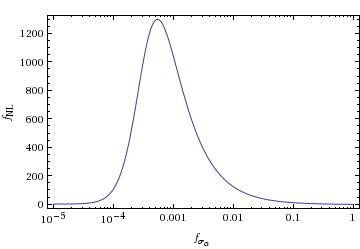
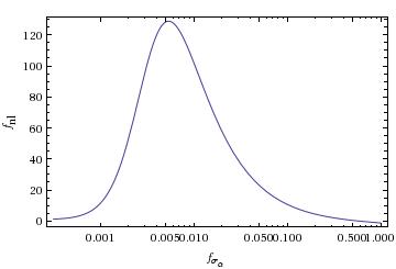
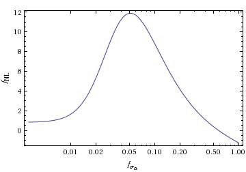
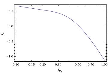
In the situation where there are two curvatons and no inflaton, the non-gaussianity depends upon the ratio of the two expectation values of the curvatons. In this case of one inflaton and one curvaton, the expression for fN​Lsubscript𝑓𝑁𝐿f_{NL} depends on the curvaton expectation value; we study it for Οƒβˆ—=1014​G​e​Vsubscript𝜎superscript1014𝐺𝑒𝑉\sigma_{*}=10^{14}GeV,Οƒβˆ—=1015​G​e​Vsubscript𝜎superscript1015𝐺𝑒𝑉\sigma_{*}=10^{15}GeV, Οƒβˆ—=1016​G​e​Vsubscript𝜎superscript1016𝐺𝑒𝑉\sigma_{*}=10^{16}GeV and Οƒβˆ—=1017​G​e​Vsubscript𝜎superscript1017𝐺𝑒𝑉\sigma_{*}=10^{17}GeV in plots Β 1 and Β 2.

Refer to caption Refer to caption
Figure 1: The non-gaussianity fN​Lsubscript𝑓𝑁𝐿f_{NL} for fΟƒΞ±βˆˆ[0,1]subscript𝑓subscriptπœŽπ›Ό01f_{\sigma_{\alpha}}\in[0,1], for Οƒβˆ—=1015​G​e​Vsubscript𝜎superscript1015𝐺𝑒𝑉\sigma_{*}=10^{15}GeV and Οƒβˆ—=1016​G​e​Vsubscript𝜎superscript1016𝐺𝑒𝑉\sigma_{*}=10^{16}GeV in the 1 inflaton-1 curvaton model.
Refer to caption Refer to caption
Figure 2: The non-gaussianity fN​Lsubscript𝑓𝑁𝐿f_{NL} for fΟƒΞ±βˆˆ[0,1]subscript𝑓subscriptπœŽπ›Ό01f_{\sigma_{\alpha}}\in[0,1], for Οƒβˆ—=1016​G​e​Vsubscript𝜎superscript1016𝐺𝑒𝑉\sigma_{*}=10^{16}GeV on the left and Οƒβˆ—=1017​G​e​Vsubscript𝜎superscript1017𝐺𝑒𝑉\sigma_{*}=10^{17}GeV on the right in the 1 inflaton-1 curvaton model.

For the first three cases we notice that the non-gaussianity increases as fσαsubscript𝑓subscriptπœŽπ›Όf_{\sigma_{\alpha}} becomes smaller, but not indefinitely. Instead, fN​Lsubscript𝑓𝑁𝐿f_{NL} has a maximum value of fN​Lm​a​x=1298subscriptsubscriptπ‘“π‘πΏπ‘šπ‘Žπ‘₯1298{f_{NL}}_{max}=1298, fN​Lm​a​x=128.8subscriptsubscriptπ‘“π‘πΏπ‘šπ‘Žπ‘₯128.8{f_{NL}}_{max}=128.8 and fN​Lm​a​x=11.9subscriptsubscriptπ‘“π‘πΏπ‘šπ‘Žπ‘₯11.9{f_{NL}}_{max}=11.9 respectively. So if we were to observe a non-gaussianity of fN​L=50subscript𝑓𝑁𝐿50f_{NL}=50 which we were to try to interpret in terms of mixed perturbations from a single inflaton and a single curvaton both with harmonic potentials, there would be two combinations of mass/decay time which would correspond to the same fN​Lsubscript𝑓𝑁𝐿f_{NL}. For Οƒβˆ—=1017​G​e​Vsubscript𝜎superscript1017𝐺𝑒𝑉\sigma_{*}=10^{17}GeV we see in Figure Β 2 that the non-gaussianity starts from values around -1 and as fσαsubscript𝑓subscriptπœŽπ›Όf_{\sigma_{\alpha}} becomes smaller it increases and reaches a maximum of fN​Lm​a​x=0.83subscriptsubscriptπ‘“π‘πΏπ‘šπ‘Žπ‘₯0.83{f_{NL}}_{max}=0.83 around which it then stays constant.

This is the same model as the one studied recently in [17]; we see the same capacity of the model to produce large values of fN​Lsubscript𝑓𝑁𝐿f_{NL} and the same increase of the non-gaussianity parameter when the curvaton expectation value becomes smaller. We also find that fN​Lsubscript𝑓𝑁𝐿f_{NL} has a maximum possible value and it in fact returns to the region allowed by observations after fσαsubscript𝑓subscriptπœŽπ›Όf_{\sigma_{\alpha}} is smaller than 2Γ—10βˆ’32superscript1032\times 10^{-3} for Οƒ=1015​G​e​V𝜎superscript1015𝐺𝑒𝑉\sigma=10^{15}GeV. Our Figures Β 1 and Β 2 are in agreement with their Fig. 2.

3.1.3 Case 1 with simultaneous decay

We would like to put some numbers into our equations to see what they are telling us. In this section, we will evaluate the fN​Lsubscript𝑓𝑁𝐿f_{NL} under the simplifying assumption that the second and third decay of case 1 happen simultaneously. Furthermore, we assume that both curvatons have a perfectly quadratic potential so that c​cβ€²β€²/c′⁣2=0𝑐superscript𝑐′′superscript𝑐′20cc^{\prime\prime}/c^{\prime 2}=0 and d​dβ€²β€²/d′⁣2=0𝑑superscript𝑑′′superscript𝑑′20dd^{\prime\prime}/d^{\prime 2}=0. To completely simplify the situation we assume that the two curvatons have equal expectation values at horizon crossing, Οƒβˆ—=Ο‡βˆ—subscript𝜎subscriptπœ’\sigma_{*}=\chi_{*}. In our plots for fN​Lsubscript𝑓𝑁𝐿f_{NL} we use the reduced Planck mass MP​l=2.4Γ—1018​G​e​Vsubscript𝑀𝑃𝑙2.4superscript1018𝐺𝑒𝑉M_{Pl}=2.4\times 10^{18}GeV and the slow roll parameter Ο΅βˆ—β‰ˆ0.02subscriptitalic-Ο΅0.02\epsilon_{*}\approx 0.02.

After the inflaton Ο•italic-Ο•\phi decays, the two curvatons decay simultaneously, Ωχ​α=Ωχ​βsubscriptΞ©πœ’π›ΌsubscriptΞ©πœ’π›½\Omega_{\chi\alpha}=\Omega_{\chi\beta}. This means that tΞ±=tΞ²subscript𝑑𝛼subscript𝑑𝛽t_{\alpha}=t_{\beta}, but to remain consistent with our notation we will express the curvature perturbation coefficients in terms of fσαsubscript𝑓subscriptπœŽπ›Όf_{\sigma_{\alpha}} and fχβsubscript𝑓subscriptπœ’π›½f_{\chi_{\beta}}. In reference [16], we find that for simultaneous decay of the two curvatons the following equation holds:

fχα=(1+fσα3)​fχβ.subscript𝑓subscriptπœ’π›Ό1subscript𝑓subscriptπœŽπ›Ό3subscript𝑓subscriptπœ’π›½f_{\chi_{\alpha}}=(1+\frac{f_{\sigma_{\alpha}}}{3})f_{\chi_{\beta}}. (42)

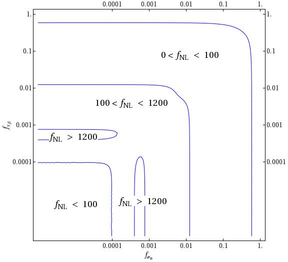
which immediately significantly simplifies the nine coefficients (A,B,ΓΓ\Gamma…) in the expression for ΢𝜁\zeta (3). The expression above is a direct result of the fact that we can consider the value of fχαsubscript𝑓subscriptπœ’π›Όf_{\chi_{\alpha}} as constrained by the given values of fσαsubscript𝑓subscriptπœŽπ›Όf_{\sigma_{\alpha}} and fχβsubscript𝑓subscriptπœ’π›½f_{\chi_{\beta}}. Since fΞ³0​α+fσα+fχα=1subscript𝑓subscript𝛾0𝛼subscript𝑓subscriptπœŽπ›Όsubscript𝑓subscriptπœ’π›Ό1f_{\gamma_{0}\alpha}+f_{\sigma_{\alpha}}+f_{\chi_{\alpha}}=1 we can write the inequality fχα≀1βˆ’fσαsubscript𝑓subscriptπœ’π›Ό1subscript𝑓subscriptπœŽπ›Όf_{\chi_{\alpha}}\leq 1-f_{\sigma_{\alpha}} and this eventually leads to fχα≀(1+fσα3)​fχβsubscript𝑓subscriptπœ’π›Ό1subscript𝑓subscriptπœŽπ›Ό3subscript𝑓subscriptπœ’π›½f_{\chi_{\alpha}}\leq(1+\frac{f_{\sigma_{\alpha}}}{3})f_{\chi_{\beta}} which is valid for all configurations. We use the simplified coefficients from equations (A-6) to (A-14) and equation (9) to obtain Figure Β 3 for fΟƒΞ±βˆˆ[0,1]subscript𝑓subscriptπœŽπ›Ό01f_{\sigma_{\alpha}}\in[0,1] and fΟ‡Ξ²βˆˆ[0,1]subscript𝑓subscriptπœ’π›½01f_{\chi_{\beta}}\in[0,1].

Refer to caption Refer to caption
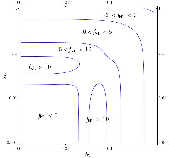
Figure 3: Contours for fN​L​(fσα,fχβ)subscript𝑓𝑁𝐿subscript𝑓subscriptπœŽπ›Όsubscript𝑓subscriptπœ’π›½f_{NL}(f_{\sigma_{\alpha}},f_{\chi_{\beta}}) as predicted in a simplified version of Case 1 for Οƒβˆ—=1014​G​e​Vsubscript𝜎superscript1014𝐺𝑒𝑉\sigma_{*}=10^{14}GeV, fΟƒΞ±βˆˆ[0,1]subscript𝑓subscriptπœŽπ›Ό01f_{\sigma_{\alpha}}\in[0,1] and fΟ‡Ξ²βˆˆ[0,1]subscript𝑓subscriptπœ’π›½01f_{\chi_{\beta}}\in[0,1] on the left. In the second plot, Οƒβˆ—=1016​G​e​Vsubscript𝜎superscript1016𝐺𝑒𝑉\sigma_{*}=10^{16}GeV while the range is fΟƒΞ±βˆˆ[10βˆ’3,1]subscript𝑓subscriptπœŽπ›Όsuperscript1031f_{\sigma_{\alpha}}\in[10^{-3},1] and fΟ‡Ξ²βˆˆ[10βˆ’3,1]subscript𝑓subscriptπœ’π›½superscript1031f_{\chi_{\beta}}\in[10^{-3},1].

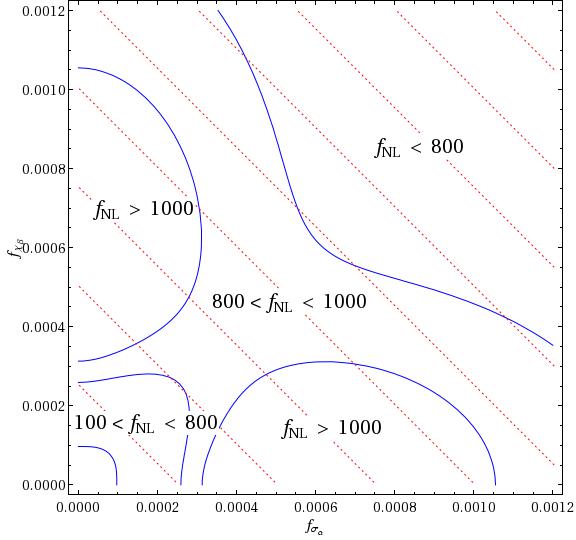
For Οƒβˆ—=1014​G​e​Vsubscript𝜎superscript1014𝐺𝑒𝑉\sigma_{*}=10^{14}GeV, we find that the maximum value for the non-linearity parameter is fN​Lm​a​x=1298subscriptsubscriptπ‘“π‘πΏπ‘šπ‘Žπ‘₯1298{f_{NL}}_{max}=1298. This value of fN​Lsubscript𝑓𝑁𝐿f_{NL} is obtained when fχβsubscript𝑓subscriptπœ’π›½f_{\chi_{\beta}} goes to zero (or alternatively fσα→0β†’subscript𝑓subscriptπœŽπ›Ό0f_{\sigma_{\alpha}}\rightarrow 0 since this case is symmetric), while the contribution of the other curvaton is ∼5Γ—10βˆ’4similar-toabsent5superscript104\sim 5\times 10^{-4}. This is precisely the same maximum value of fN​Lsubscript𝑓𝑁𝐿f_{NL} as the one in Figure Β 1 where we studied a model with one inflaton and one curvaton, as would be expected.It’s the same in the case of Οƒβˆ—=1016​G​e​Vsubscript𝜎superscript1016𝐺𝑒𝑉\sigma_{*}=10^{16}GeV; we find that the maximum value of the non-gaussianity is fN​Lm​a​x=11.9subscriptsubscriptπ‘“π‘πΏπ‘šπ‘Žπ‘₯11.9{f_{NL}}_{max}=11.9 and is identical to the result we got in the 1 inflaton 1 curvaton case. This maximum value is not observed in the non-gaussianity produced in the two curvaton scenario as studied in [16]. The only difference between our Case 1 and the model in [16] is the inclusion of the inflaton’s contribution to the perturbations in our work, which creates an upper boundary for fN​Lsubscript𝑓𝑁𝐿f_{NL}.

It is evident in all our plots that there are many different combinations of fσαsubscript𝑓subscriptπœŽπ›Όf_{\sigma_{\alpha}} and fχβsubscript𝑓subscriptπœ’π›½f_{\chi_{\beta}} that can give the same prediction for non-gaussianity. On the other hand, we want to emphasise with Figure Β 4, that even when we keep the total contribution of the curvatons to the perturbation constant (red dashed lines), the fN​Lsubscript𝑓𝑁𝐿f_{NL} can still change significantly.

Refer to caption
Figure 4: The area of large fN​Lsubscript𝑓𝑁𝐿f_{NL} in case 1 for Οƒβˆ—=1014​G​e​Vsubscript𝜎superscript1014𝐺𝑒𝑉\sigma_{*}=10^{14}GeV. The red dashed lines correspond to fσα+fχβ=constantsubscript𝑓subscriptπœŽπ›Όsubscript𝑓subscriptπœ’π›½constantf_{\sigma_{\alpha}}+f_{\chi_{\beta}}=\textrm{constant}.

3.2 Case 2: tΟƒo​s​c<tΟ‡o​s​c<tΟƒd​e​c​a​y<tΟ•d​e​c​a​y<tΟ‡d​e​c​a​ysubscript𝑑subscriptπœŽπ‘œπ‘ π‘subscript𝑑subscriptπœ’π‘œπ‘ π‘subscript𝑑subscriptπœŽπ‘‘π‘’π‘π‘Žπ‘¦subscript𝑑subscriptitalic-Ο•π‘‘π‘’π‘π‘Žπ‘¦subscript𝑑subscriptπœ’π‘‘π‘’π‘π‘Žπ‘¦t_{\sigma_{osc}}<t_{\chi_{osc}}<t_{\sigma_{decay}}<t_{\phi_{decay}}<t_{\chi_{decay}}

For the second case, we assume that one of the curvatons decays early, before the inflaton. Following the same procedure as in the first case we write down an equation valid just before the inflaton decays (decay 1):

Ωγ0​α​e4​(ΞΆΟƒβˆ’ΞΆΞ±)+Ωϕ1​e3​(ΞΆΟ•βˆ’ΞΆΞ±)+Ωχ​α​e3​(ΞΆΟ‡βˆ’ΞΆΞ±)=1.subscriptΞ©subscript𝛾0𝛼superscript𝑒4subscript𝜁𝜎subscriptπœπ›ΌsubscriptΞ©subscriptitalic-Ο•1superscript𝑒3subscript𝜁italic-Ο•subscriptπœπ›ΌsubscriptΞ©πœ’π›Όsuperscript𝑒3subscriptπœπœ’subscriptπœπ›Ό1\Omega_{\gamma_{0}\alpha}e^{4(\zeta_{\sigma}-\zeta_{\alpha})}+\Omega_{\phi_{1}}e^{3(\zeta_{\phi}-\zeta_{\alpha})}+\Omega_{\chi\alpha}e^{3(\zeta_{\chi}-\zeta_{\alpha})}=1. (43)

Here, the energy density of the curvaton ΟƒπœŽ\sigma, which has decayed, forms the background radiation Ξ³0subscript𝛾0\gamma_{0}, while the other two particles are still oscillating so their energy density evolves like matter. This means that in what follows in this section, Ωγ0​α=Ωσ​αsubscriptΞ©subscript𝛾0𝛼subscriptΞ©πœŽπ›Ό\Omega_{\gamma_{0}\alpha}=\Omega_{\sigma\alpha} and fΞ³0​α=fσα=1βˆ’fΟ•Ξ±βˆ’fχαsubscript𝑓subscript𝛾0𝛼subscript𝑓subscriptπœŽπ›Ό1subscript𝑓subscriptitalic-ϕ𝛼subscript𝑓subscriptπœ’π›Όf_{\gamma_{0\alpha}}=f_{\sigma_{\alpha}}=1-f_{\phi_{\alpha}}-f_{\chi_{\alpha}}. Once the inflaton decays as well, we have

Ωγ1​α​e4​(ΞΆΞ³1βˆ’ΞΆΞ±)+Ωχ​α​e3​(ΞΆΟ‡βˆ’ΞΆΞ±)=1subscriptΞ©subscript𝛾1𝛼superscript𝑒4subscript𝜁subscript𝛾1subscriptπœπ›ΌsubscriptΞ©πœ’π›Όsuperscript𝑒3subscriptπœπœ’subscriptπœπ›Ό1\Omega_{\gamma_{1}\alpha}e^{4(\zeta_{\gamma_{1}}-\zeta_{\alpha})}+\Omega_{\chi\alpha}e^{3(\zeta_{\chi}-\zeta_{\alpha})}=1 (44)

where the energy densities of Ο•italic-Ο•\phi and ΟƒπœŽ\sigma have been converted to radiation, and we see that the system is now the same as in the first case: the inflaton and one curvaton have decayed into radiation, while the second curvaton oscillates. This means that in this case the equations valid before and after the last decay are simply (24) and (25) respectively. To obtain the coefficients present in the non-gaussianity expression (9), we need the first and second order components of the curvature perturbation at the last decay. Just like we did in the previous case we expand the equations above to second order, to eventually get

ΞΆΞ²subscriptπœπ›½\displaystyle\zeta_{\beta} =\displaystyle= R1​fΟ•1​(1βˆ’fχβ)​΢ϕ(1)+R1​fσα​(1βˆ’fχβ)​΢σ(1)subscript𝑅1subscript𝑓subscriptitalic-Ο•11subscript𝑓subscriptπœ’π›½subscriptsubscript𝜁italic-Ο•1subscript𝑅1subscript𝑓subscriptπœŽπ›Ό1subscript𝑓subscriptπœ’π›½subscriptsubscript𝜁𝜎1\displaystyle R_{1}f_{\phi_{1}}(1-f_{\chi_{\beta}}){\zeta_{\phi}}_{(1)}+R_{1}f_{\sigma_{\alpha}}(1-f_{\chi_{\beta}}){\zeta_{\sigma}}_{(1)} (45)
+[1βˆ’R1​(1βˆ’fχα)​(1βˆ’fχβ)]​΢χ(1)+4​(1βˆ’fχβ)​(ΞΆΞ³1(1)βˆ’ΞΆΞ²(1))2delimited-[]1subscript𝑅11subscript𝑓subscriptπœ’π›Ό1subscript𝑓subscriptπœ’π›½subscriptsubscriptπœπœ’141subscript𝑓subscriptπœ’π›½superscriptsubscriptsubscript𝜁subscript𝛾11subscriptsubscriptπœπ›½12\displaystyle+[1-R_{1}(1-f_{\chi_{\alpha}})(1-f_{\chi_{\beta}})]{\zeta_{\chi}}_{(1)}+4(1-f_{\chi_{\beta}})({\zeta_{\gamma_{1}}}_{(1)}-{\zeta_{\beta}}_{(1)})^{2}
+3​fχβ​(ΞΆΟ‡(1)βˆ’ΞΆΞ²(1))2+(1βˆ’fχβ)​΢γ1(2)+fχβ​΢χ(2),3subscript𝑓subscriptπœ’π›½superscriptsubscriptsubscriptπœπœ’1subscriptsubscriptπœπ›½121subscript𝑓subscriptπœ’π›½subscriptsubscript𝜁subscript𝛾12subscript𝑓subscriptπœ’π›½subscriptsubscriptπœπœ’2\displaystyle+3f_{\chi_{\beta}}({\zeta_{\chi}}_{(1)}-{\zeta_{\beta}}_{(1)})^{2}+(1-f_{\chi_{\beta}}){\zeta_{\gamma_{1}}}_{(2)}+f_{\chi_{\beta}}{\zeta_{\chi}}_{(2)},

which we can rewrite solely in terms of ΞΆΟ•1(1)subscriptsubscript𝜁subscriptitalic-Ο•11{\zeta_{\phi_{1}}}_{(1)}, SΟƒ(1)subscriptsubscriptπ‘†πœŽ1{S_{\sigma}}_{(1)} and SΟ‡(1)subscriptsubscriptπ‘†πœ’1{S_{\chi}}_{(1)} to read off the curvature perturbation coefficients. The list can be found in equations (A-15)-(A-23) in the Appendix.

3.2.1 Case 2 with simultaneous decay

Again, we would like to evaluate our equations to find out what new information they are giving us.

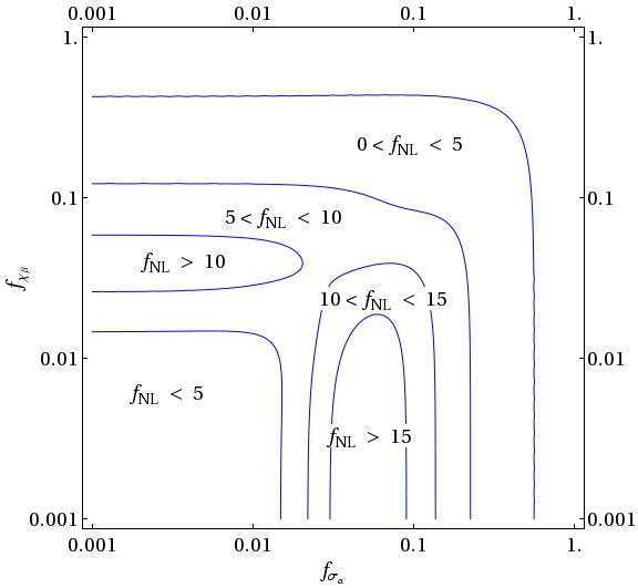
In this case we assume that after curvaton ΟƒπœŽ\sigma decays, the inflaton and the other curvaton decay at the same time. The coefficients in the curvature perturbation expression written in terms of fσαsubscript𝑓subscriptπœŽπ›Όf_{\sigma_{\alpha}} and fχβsubscript𝑓subscriptπœ’π›½f_{\chi_{\beta}} can be obtained by placing the relation fΞ³0​α=fσα=1βˆ’fΟ•Ξ±βˆ’fχαsubscript𝑓subscript𝛾0𝛼subscript𝑓subscriptπœŽπ›Ό1subscript𝑓subscriptitalic-ϕ𝛼subscript𝑓subscriptπœ’π›Όf_{\gamma_{0\alpha}}=f_{\sigma_{\alpha}}=1-f_{\phi_{\alpha}}-f_{\chi_{\alpha}} into equations (A-15)-(A-23) to produce equations (A-24) to (A-32). We then create contour plots of our expression for fN​Lsubscript𝑓𝑁𝐿f_{NL} in Figure Β 5. The maximum value for fN​Lsubscript𝑓𝑁𝐿f_{NL} is fN​Lm​a​x=2162.5subscriptsubscriptπ‘“π‘πΏπ‘šπ‘Žπ‘₯2162.5{f_{NL}}_{max}=2162.5 for Οƒβˆ—=1014​G​e​Vsubscript𝜎superscript1014𝐺𝑒𝑉\sigma_{*}=10^{14}GeV. This is significantly larger than the maximum fN​Lsubscript𝑓𝑁𝐿f_{NL} value of Case 1, which shows that the order of the particles’ decay can have a big effect on non-gaussianity.
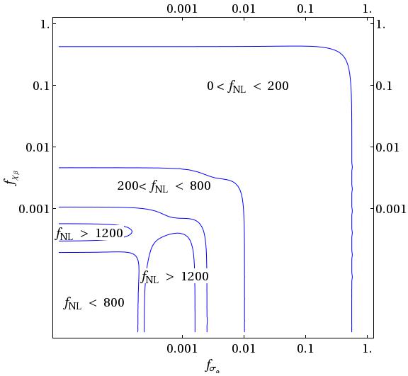
Refer to caption Refer to caption
Figure 5: fN​Lsubscript𝑓𝑁𝐿f_{NL} in Case 2 when the second and third decay happen simultaneously, in terms of fσαsubscript𝑓subscriptπœŽπ›Όf_{\sigma_{\alpha}} and fχβsubscript𝑓subscriptπœ’π›½f_{\chi_{\beta}}. The plot on the left is done for Οƒβˆ—=1014​G​e​Vsubscript𝜎superscript1014𝐺𝑒𝑉\sigma_{*}=10^{14}GeV with fΟƒΞ±βˆˆ[0,1]subscript𝑓subscriptπœŽπ›Ό01f_{\sigma_{\alpha}}\in[0,1] and fΟ‡Ξ²βˆˆ[0,1]subscript𝑓subscriptπœ’π›½01f_{\chi_{\beta}}\in[0,1], while the plot on the right for Οƒβˆ—=1016​G​e​Vsubscript𝜎superscript1016𝐺𝑒𝑉\sigma_{*}=10^{16}GeV with fΟƒΞ±βˆˆ[10βˆ’3,1]subscript𝑓subscriptπœŽπ›Όsuperscript1031f_{\sigma_{\alpha}}\in[10^{-3},1] and fΟ‡Ξ²βˆˆ[10βˆ’3,1]subscript𝑓subscriptπœ’π›½superscript1031f_{\chi_{\beta}}\in[10^{-3},1].

We see that the prediction for fN​Lsubscript𝑓𝑁𝐿f_{NL} is significantly smaller for larger Οƒβˆ—subscript𝜎\sigma_{*}. In the case where Οƒβˆ—=1016​G​e​Vsubscript𝜎superscript1016𝐺𝑒𝑉\sigma_{*}=10^{16}GeV we find the maximum value fN​Lm​a​x=19.2subscriptsubscriptπ‘“π‘πΏπ‘šπ‘Žπ‘₯19.2{f_{NL}}_{max}=19.2.

3.3 Case 3: tΟƒo​s​c<tΟ‡o​s​c<tΟƒd​e​c​a​y<tΟ‡d​e​c​a​y<tΟ•d​e​c​a​ysubscript𝑑subscriptπœŽπ‘œπ‘ π‘subscript𝑑subscriptπœ’π‘œπ‘ π‘subscript𝑑subscriptπœŽπ‘‘π‘’π‘π‘Žπ‘¦subscript𝑑subscriptπœ’π‘‘π‘’π‘π‘Žπ‘¦subscript𝑑subscriptitalic-Ο•π‘‘π‘’π‘π‘Žπ‘¦t_{\sigma_{osc}}<t_{\chi_{osc}}<t_{\sigma_{decay}}<t_{\chi_{decay}}<t_{\phi_{decay}}

In the third scenario, we consider a late decaying inflaton, decaying after both the curvatons have oscillated and decayed. The decay of the curvaton ΟƒπœŽ\sigma creates the radiation fluid present just before the decay of Ο‡πœ’\chi:

Ωγ0​α​e4​(ΞΆΟƒβˆ’ΞΆΞ±)+Ωχ​α​e3​(ΞΆΟ‡βˆ’ΞΆΞ±)+Ωϕ1​e3​(ΞΆΟ•βˆ’ΞΆΞ±)=1.subscriptΞ©subscript𝛾0𝛼superscript𝑒4subscript𝜁𝜎subscriptπœπ›ΌsubscriptΞ©πœ’π›Όsuperscript𝑒3subscriptπœπœ’subscriptπœπ›ΌsubscriptΞ©subscriptitalic-Ο•1superscript𝑒3subscript𝜁italic-Ο•subscriptπœπ›Ό1\Omega_{\gamma_{0}\alpha}e^{4(\zeta_{\sigma}-\zeta_{\alpha})}+\Omega_{\chi\alpha}e^{3(\zeta_{\chi}-\zeta_{\alpha})}+\Omega_{\phi_{1}}e^{3(\zeta_{\phi}-\zeta_{\alpha})}=1. (46)

After the second curvaton decays as well, we have:

Ωγ1​α​e4​(ΞΆΞ³1βˆ’ΞΆΞ±)+Ωϕ1​e3​(ΞΆΟ•βˆ’ΞΆΞ±)=1.subscriptΞ©subscript𝛾1𝛼superscript𝑒4subscript𝜁subscript𝛾1subscriptπœπ›ΌsubscriptΞ©subscriptitalic-Ο•1superscript𝑒3subscript𝜁italic-Ο•subscriptπœπ›Ό1\Omega_{\gamma_{1}\alpha}e^{4(\zeta_{\gamma_{1}}-\zeta_{\alpha})}+\Omega_{\phi_{1}}e^{3(\zeta_{\phi}-\zeta_{\alpha})}=1. (47)

We can also write the following two equations valid before and after the last decay:

Ωγ1​β​e4​(ΞΆΞ³1βˆ’ΞΆΞ²)+Ωϕ1​e3​(ΞΆΟ•βˆ’ΞΆΞ²)subscriptΞ©subscript𝛾1𝛽superscript𝑒4subscript𝜁subscript𝛾1subscriptπœπ›½subscriptΞ©subscriptitalic-Ο•1superscript𝑒3subscript𝜁italic-Ο•subscriptπœπ›½\displaystyle\Omega_{\gamma_{1}\beta}e^{4(\zeta_{\gamma_{1}}-\zeta_{\beta})}+\Omega_{\phi_{1}}e^{3(\zeta_{\phi}-\zeta_{\beta})} =\displaystyle= 11\displaystyle 1 (48)
Ωγ2​β​e4​(ΞΆΞ³2βˆ’ΞΆΞ²)subscriptΞ©subscript𝛾2𝛽superscript𝑒4subscript𝜁subscript𝛾2subscriptπœπ›½\displaystyle\Omega_{\gamma_{2}\beta}e^{4(\zeta_{\gamma_{2}}-\zeta_{\beta})} =\displaystyle= 1.1\displaystyle 1. (49)

These are the four main equations for this case and expanding them to second order eventually results in the expression for the primordial curvature perturbation at the time of last decay

ΞΆΞ²subscriptπœπ›½\displaystyle\zeta_{\beta} =\displaystyle= [1βˆ’R1​(1βˆ’fϕα)​(1βˆ’fϕβ)]​΢ϕ(1)+R1​fσα​(1βˆ’fϕβ)​΢σ(1)delimited-[]1subscript𝑅11subscript𝑓subscriptitalic-ϕ𝛼1subscript𝑓subscriptitalic-ϕ𝛽subscriptsubscript𝜁italic-Ο•1subscript𝑅1subscript𝑓subscriptπœŽπ›Ό1subscript𝑓subscriptitalic-ϕ𝛽subscriptsubscript𝜁𝜎1\displaystyle[1-R_{1}(1-f_{\phi_{\alpha}})(1-f_{\phi_{\beta}})]{\zeta_{\phi}}_{(1)}+R_{1}f_{\sigma_{\alpha}}(1-f_{\phi_{\beta}}){\zeta_{\sigma}}_{(1)} (50)
+R1​fχα​(1βˆ’fϕβ)​΢χ(1)+4​fϕβ​(ΞΆΞ³1(1)βˆ’ΞΆΞ²(1))2subscript𝑅1subscript𝑓subscriptπœ’π›Ό1subscript𝑓subscriptitalic-ϕ𝛽subscriptsubscriptπœπœ’14subscript𝑓subscriptitalic-ϕ𝛽superscriptsubscriptsubscript𝜁subscript𝛾11subscriptsubscriptπœπ›½12\displaystyle+R_{1}f_{\chi_{\alpha}}(1-f_{\phi_{\beta}}){\zeta_{\chi}}_{(1)}+4f_{\phi_{\beta}}({\zeta_{\gamma_{1}}}_{(1)}-{\zeta_{\beta}}_{(1)})^{2}
+3​(1βˆ’fϕβ)​(ΞΆΟ•(1)βˆ’ΞΆΞ²(1))2+fϕβ​΢γ1(2)+(1βˆ’fϕβ)​΢ϕ(2)31subscript𝑓subscriptitalic-ϕ𝛽superscriptsubscriptsubscript𝜁italic-Ο•1subscriptsubscriptπœπ›½12subscript𝑓subscriptitalic-ϕ𝛽subscriptsubscript𝜁subscript𝛾121subscript𝑓subscriptitalic-ϕ𝛽subscriptsubscript𝜁italic-Ο•2\displaystyle+3(1-f_{\phi_{\beta}})({\zeta_{\phi}}_{(1)}-{\zeta_{\beta}}_{(1)})^{2}+f_{\phi_{\beta}}{\zeta_{\gamma_{1}}}_{(2)}+(1-f_{\phi_{\beta}}){\zeta_{\phi}}_{(2)}

We rewrite this to match the form of equation (3). We list the resulting nine coefficients in the Appendix.

Case 3, in the simultaneous decay limit is equivalent to Case 2 for b↔ϕ↔𝑏italic-Ο•b\leftrightarrow\phi.

4 Discussion

In this work, we have studied the non-gaussianity predicted in models of inflation with 1 inflaton and 2 curvatons. We derived a general expression for fN​Lsubscript𝑓𝑁𝐿f_{NL} from the bi-spectrum of a general curvature perturbation ΢𝜁\zeta. We saw that our general expression simplifies to reproduce other expressions for fN​Lsubscript𝑓𝑁𝐿f_{NL} in the literature under the relevant simplifications.

We then analytically derived the necessary coefficients for specific scenarios in which we varied the sequence of the decays of the three particle species. For our main three cases, we then simplified our fN​Lsubscript𝑓𝑁𝐿f_{NL} expression under the assumption that the last two decays happen at the same time.

For all of the calculations we performed in this paper, we assumed a harmonic potential for the inflaton of the form m2​ϕ2superscriptπ‘š2superscriptitalic-Ο•2m^{2}\phi^{2} and we assumed therefore a slow roll parameter 60 efolds before the end of inflation of ϡ∼0.02similar-toitalic-Ο΅0.02\epsilon\sim 0.02. We made no assumption for the potential of the curvatons in our general calculations; for the simplified cases we used the quadratic form.

In the simultaneous decay limit we studied the features of the predicted fN​Lsubscript𝑓𝑁𝐿f_{NL} and found that the produced non-gaussianity is bounded. When the contribution of the curvaton to the final perturbation is of order unity, fN​Lsubscript𝑓𝑁𝐿f_{NL} is slightly negative but becomes more positive as fσαsubscript𝑓subscriptπœŽπ›Όf_{\sigma_{\alpha}} and fχβsubscript𝑓subscriptπœ’π›½f_{\chi_{\beta}} become smaller. The maximum value of fN​Lsubscript𝑓𝑁𝐿f_{NL} is set in this situation by the expectation value Οƒβˆ—subscript𝜎\sigma_{*} of the curvaton during inflation and is smaller when Οƒβˆ—subscript𝜎\sigma_{*} is larger. For expectation values smaller than around 1016superscript101610^{16} GeV fN​Lsubscript𝑓𝑁𝐿f_{NL} grows beyond the current observational constraints if the relative contribution of the curvaton has the right value. If the expectation value of the curvaton is 1017superscript101710^{17} GeV then we find that the maximum non-gaussianity is around fN​L∼0.8similar-tosubscript𝑓𝑁𝐿0.8f_{NL}\sim 0.8 which is not in the range that will be detectable by Planck.

We find that fN​Lsubscript𝑓𝑁𝐿f_{NL} can take very large values, depending upon the expectation value of the curvaton during inflation but that it does not grow indefinitely. After it reaches a maximum it decreases and returns to within the range allowed by current observations.

A particular value of fN​Lsubscript𝑓𝑁𝐿f_{NL} therefore corresponds to two different sets of parameters, even in the situation where there is a single inflaton and a single curvaton and more information is required.

The predicted fN​Lsubscript𝑓𝑁𝐿f_{NL} in all of the three field models in this paper is quite a complicated function of the relative contributions of the two curvatons. If, for example, we take the situation where 80% of the total curvature perturbation comes from the inflaton and 20% comes from the combined effect of the two curvatons, there are situations where having all of the curvaton contribution to the pertubation coming from one of the two curvaton fields will maximise fN​Lsubscript𝑓𝑁𝐿f_{NL}, and there are situations where having 10% of the perturbation coming from each curvaton will maximise fN​Lsubscript𝑓𝑁𝐿f_{NL}, depending upon the expectation values of the curvaton fields. There are therefore in general several combinations of field parameters that give the same non-gaussianity and, alternatively, even when these parameters change in a way that leaves the total curvaton contribution to ΢𝜁\zeta constant there can be big changes in the value of fN​Lsubscript𝑓𝑁𝐿f_{NL}.

Of course it would be interesting therefore to investigate the trispectrum to see if the parameter gN​Lsubscript𝑔𝑁𝐿g_{NL} could contribute to distinguishing between different models. It is also quite clear that the machinery used in this paper leads to rather a lot of long equations. It would be nice to come up with a way of simplifying the calculations such that one could make more general statements about N curvatons.

Acknowledgments

MF is very grateful for funding from the STFC. We are also very happy to thank Karim Malik, Filippo Vernizzi and David Wands.

References

  • [1] A. R. Liddle, astro-ph/9901124v1
  • [2] G. Lazarides, hep-ph/9802415v2
  • [3] A. R. Liddle, D. H. Lyth, Phys. Rep.πŸπŸ‘πŸ231\mathbf{231}, 1 (1993), astro-ph/9303019
  • [4] D. H. Lyth, D. Wands,Phys. Let. BπŸ“πŸπŸ’524\mathbf{524} (2002), hep-ph/0110002v2
  • [5] D. H. Lyth, C. Ungarelli, D. Wands, Phys. Rev. DπŸ”πŸ•67\mathbf{67}, astro-ph/0208055v3
  • [6] N. Bartolo, A. R. Liddle, Phys. Rev. D πŸ”πŸ“65\mathbf{65},astro-ph/0203076v2
  • [7] D. Wands, K. Malik, D. H. Lyth, A. R. Liddle, Phys. Rev. 62 (2000), astro-ph/0003278v2
  • [8] C. T. Byrnes, K. Choi, astro-ph/1002.3110v2
  • [9] D. Wands, astro-ph/1004.0818v1
  • [10] K. Dimopoulos, G. Lazarides, D.. H. Lyth, R. R. de Austri, hep-ph/0308015v1
  • [11] D. Langlois, astro-ph/1102.5052v1
  • [12] N. Bartolo, S. Matarrese, A. Riotto, Phys. Rev. DπŸ”πŸ—69\mathbf{69} (2004), hep-ph/0309033v3
  • [13] C. Gordon, A. Lewis, astro-ph/0212248v3
  • [14] E. Komatsu, astro-ph/1003.6097v2
  • [15] E. Komatsu π‘’π‘‘β€‹Β β€‹π‘Žπ‘™.π‘’π‘‘Β π‘Žπ‘™\mathit{et\textrm{ }al.} [WMAP Collaboration], arXiv:1001.4538
  • [16] H. Assadullahi, J. Valiviita, D. Wands, Phys. Rev. DπŸ•πŸ”76\mathbf{76} hep-ph/0708.0223v1
  • [17] J. Fonseca, D. Wands, astro-ph/1204.3443v2
  • [18] D. Lyth, K. Malik, M. Sasaki, JCAP 0505:004, 2005, astro-ph/0411220v
  • [19] M. Sasaki, J. Valiviita, D. Wands, Phys. Rev. DπŸ•πŸ’74\mathbf{74}, astro-ph/0607627v3
  • [20] D. Lyth, Y. Rodriguez,astro-ph/0504045v4

Appendix A Appendix

A.1 Case 1

Expanding equation (25) up to second order yields:

11\displaystyle 1 =\displaystyle= Ωγ2​β[1+4(ΞΆΞ³2(1)+12ΞΆΞ³2(2)βˆ’ΞΆΞ²(1)βˆ’12ΞΆΞ²(2))\displaystyle\Omega_{\gamma_{2}\beta}[1+4({\zeta_{\gamma_{2}}}_{(1)}+\frac{1}{2}{\zeta_{\gamma_{2}}}_{(2)}-{\zeta_{\beta}}_{(1)}-\frac{1}{2}{\zeta_{\beta}}_{(2)}) (A-1)
+162(ΞΆΞ³2(1)βˆ’ΞΆΞ²(2))2].\displaystyle+\frac{16}{2}({\zeta_{\gamma_{2}}}_{(1)}-{\zeta_{\beta}}_{(2)})^{2}].

Zeroth order is just

Ωγ2​β=1subscriptΞ©subscript𝛾2𝛽1\Omega_{\gamma_{2}\beta}=1 (A-2)

which is an identity, as after the decay of the second curvaton all three particles have decayed into radiation. The first order terms give simply

ΞΆΞ²(1)=ΞΆΞ³2(1),subscriptsubscriptπœπ›½1subscriptsubscript𝜁subscript𝛾21{\zeta_{\beta}}_{(1)}={\zeta_{\gamma_{2}}}_{(1)}, (A-3)

while the second order terms give the equation

ΞΆΞ³2(2)=βˆ’2​(ΞΆΞ³2(1)βˆ’ΞΆΞ²(2))2+ΞΆΞ²(2).subscriptsubscript𝜁subscript𝛾222superscriptsubscriptsubscript𝜁subscript𝛾21subscriptsubscriptπœπ›½22subscriptsubscriptπœπ›½2{\zeta_{\gamma_{2}}}_{(2)}=-2({\zeta_{\gamma_{2}}}_{(1)}-{\zeta_{\beta}}_{(2)})^{2}+{\zeta_{\beta}}_{(2)}. (A-4)

Combining these two equations we get

ΞΆΞ³2(2)=ΞΆΞ²(2),subscriptsubscript𝜁subscript𝛾22subscriptsubscriptπœπ›½2{\zeta_{\gamma_{2}}}_{(2)}={\zeta_{\beta}}_{(2)}, (A-5)

which is consistent since all that’s left after all the particles have decayed is radiation.

A.1.1 Case 1 with simultaneous decay

Below we list the nine curvature perturbation coefficients for Case 1 when we assume that the two curvatons decay at the same time. The coefficients are given in terms of fσαsubscript𝑓subscriptπœŽπ›Όf_{\sigma_{\alpha}} and fχβsubscript𝑓subscriptπœ’π›½f_{\chi_{\beta}}.

AA\displaystyle{\rm A} =\displaystyle= 11\displaystyle 1 (A-6)
BB\displaystyle{\rm B} =\displaystyle= fσα3subscript𝑓subscriptπœŽπ›Ό3\displaystyle\frac{f_{\sigma_{\alpha}}}{3} (A-7)
ΓΓ\displaystyle\Gamma =\displaystyle= 19​(3+fσα)​fχβ193subscript𝑓subscriptπœŽπ›Όsubscript𝑓subscriptπœ’π›½\displaystyle\frac{1}{9}(3+f_{\sigma_{\alpha}})f_{\chi_{\beta}} (A-8)
ΔΔ\displaystyle\Delta =\displaystyle= 12​[βˆ’3​fΟ‡Ξ²βˆ’fσα​(3+2​fχβ)]12delimited-[]3subscript𝑓subscriptπœ’π›½subscript𝑓subscriptπœŽπ›Ό32subscript𝑓subscriptπœ’π›½\displaystyle\frac{1}{2}[-3f_{\chi_{\beta}}-f_{\sigma_{\alpha}}(3+2f_{\chi_{\beta}})] (A-9)
EE\displaystyle{\rm E} =\displaystyle= βˆ’154​fσα​[βˆ’9+6​fσα​(2+fχβ)+2​fσα2​(3+fχβ)]154subscript𝑓subscriptπœŽπ›Όdelimited-[]96subscript𝑓subscriptπœŽπ›Ό2subscript𝑓subscriptπœ’π›½2superscriptsubscript𝑓subscriptπœŽπ›Ό23subscript𝑓subscriptπœ’π›½\displaystyle-\frac{1}{54}f_{\sigma_{\alpha}}[-9+6f_{\sigma_{\alpha}}(2+f_{\chi_{\beta}})+2f_{\sigma_{\alpha}}^{2}(3+f_{\chi_{\beta}})] (A-10)
ZZ\displaystyle{\rm Z} =\displaystyle= βˆ’1486​fχβ​[βˆ’81+6​(2+fσα)​(3+fσα)2​fχβ+2​(3+fσα)3​fχβ2]1486subscript𝑓subscriptπœ’π›½delimited-[]8162subscript𝑓subscriptπœŽπ›Όsuperscript3subscript𝑓subscriptπœŽπ›Ό2subscript𝑓subscriptπœ’π›½2superscript3subscript𝑓subscriptπœŽπ›Ό3superscriptsubscript𝑓subscriptπœ’π›½2\displaystyle-\frac{1}{486}f_{\chi_{\beta}}[-81+6(2+f_{\sigma_{\alpha}})(3+f_{\sigma_{\alpha}})^{2}f_{\chi_{\beta}}+2(3+f_{\sigma_{\alpha}})^{3}f_{\chi_{\beta}}^{2}] (A-11)
HH\displaystyle{\rm H} =\displaystyle= βˆ’fσαsubscript𝑓subscriptπœŽπ›Ό\displaystyle-f_{\sigma_{\alpha}} (A-12)
ΘΘ\displaystyle\Theta =\displaystyle= βˆ’13​(3+2​fσα)​fχβ1332subscript𝑓subscriptπœŽπ›Όsubscript𝑓subscriptπœ’π›½\displaystyle-\frac{1}{3}(3+2f_{\sigma_{\alpha}})f_{\chi_{\beta}} (A-13)
II\displaystyle{\rm I} =\displaystyle= βˆ’281​fσα​(3+fσα)​fχβ​[3​(2+fχβ)+fσα​(3+fχβ)]281subscript𝑓subscriptπœŽπ›Ό3subscript𝑓subscriptπœŽπ›Όsubscript𝑓subscriptπœ’π›½delimited-[]32subscript𝑓subscriptπœ’π›½subscript𝑓subscriptπœŽπ›Ό3subscript𝑓subscriptπœ’π›½\displaystyle-\frac{2}{81}f_{\sigma_{\alpha}}(3+f_{\sigma_{\alpha}})f_{\chi_{\beta}}[3(2+f_{\chi_{\beta}})+f_{\sigma_{\alpha}}(3+f_{\chi_{\beta}})] (A-14)

A.2 Case 2

The nine coefficients needed in the fN​Lsubscript𝑓𝑁𝐿f_{NL} expresion (9) are listed below:

AA\displaystyle{\rm A} =\displaystyle= 11\displaystyle 1 (A-15)
BB\displaystyle{\rm B} =\displaystyle= 13​R1​fσα​(1βˆ’fχβ)13subscript𝑅1subscript𝑓subscriptπœŽπ›Ό1subscript𝑓subscriptπœ’π›½\displaystyle\frac{1}{3}R_{1}f_{\sigma_{\alpha}}(1-f_{\chi_{\beta}}) (A-16)
ΓΓ\displaystyle\Gamma =\displaystyle= 13​[1βˆ’R1​(1βˆ’fχα)​(1βˆ’fχβ)]13delimited-[]1subscript𝑅11subscript𝑓subscriptπœ’π›Ό1subscript𝑓subscriptπœ’π›½\displaystyle\frac{1}{3}[1-R_{1}(1-f_{\chi_{\alpha}})(1-f_{\chi_{\beta}})] (A-17)
ΔΔ\displaystyle\Delta =\displaystyle= 32[βˆ’1+R1βˆ’R1fσα(1βˆ’fχβ)βˆ’R1fχα(1βˆ’fχβ)βˆ’R1fχβ+R1fσα(1βˆ’c​cβ€²β€²c′⁣2)\displaystyle\frac{3}{2}[-1+R_{1}-R_{1}f_{\sigma_{\alpha}}(1-f_{\chi_{\beta}})-R_{1}f_{\chi_{\alpha}}(1-f_{\chi_{\beta}})-R_{1}f_{\chi_{\beta}}+R_{1}f_{\sigma_{\alpha}}(1-\frac{cc^{\prime\prime}}{c^{\prime 2}}) (A-18)
+(1βˆ’R1(1βˆ’fχα))(1βˆ’d​dβ€²β€²d′⁣2)+fχβc​cβ€²β€²c′⁣2]\displaystyle+(1-R_{1}(1-f_{\chi_{\alpha}}))(1-\frac{dd^{\prime\prime}}{d^{\prime 2}})+f_{\chi_{\beta}}\frac{cc^{\prime\prime}}{c^{\prime 2}}]
EE\displaystyle{\rm E} =\displaystyle= 118​fσα​(1βˆ’fχβ)​[5​R1+2​R1​fσα2+2​fσα​(βˆ’1βˆ’4​R12+3​R12​fχβ+R12​fχβ2)]118subscript𝑓subscriptπœŽπ›Ό1subscript𝑓subscriptπœ’π›½delimited-[]5subscript𝑅12subscript𝑅1superscriptsubscript𝑓subscriptπœŽπ›Ό22subscript𝑓subscriptπœŽπ›Ό14superscriptsubscript𝑅123superscriptsubscript𝑅12subscript𝑓subscriptπœ’π›½superscriptsubscript𝑅12superscriptsubscript𝑓subscriptπœ’π›½2\displaystyle\frac{1}{18}f_{\sigma_{\alpha}}(1-f_{\chi_{\beta}})[5R_{1}+2R_{1}f_{\sigma_{\alpha}}^{2}+2f_{\sigma_{\alpha}}(-1-4R_{1}^{2}+3R_{1}^{2}f_{\chi_{\beta}}+R_{1}^{2}f_{\chi_{\beta}}^{2})] (A-19)
+16​R1​fσα​c​cβ€²β€²c′⁣216subscript𝑅1subscript𝑓subscriptπœŽπ›Όπ‘superscript𝑐′′superscript𝑐′2\displaystyle+\frac{1}{6}R_{1}f_{\sigma_{\alpha}}\frac{cc^{\prime\prime}}{c^{\prime 2}}
ZZ\displaystyle{\rm Z} =\displaystyle= 19{βˆ’3​fχβ2+12(1βˆ’fχβ)[βˆ’5+13R1βˆ’8R12\displaystyle\frac{1}{9}\{-\frac{3f_{\chi_{\beta}}}{2}+\frac{1}{2}(1-f_{\chi_{\beta}})[-5+13R_{1}-8R_{1}^{2} (A-20)
+6R12fχβ+2R12fχβ2+fχα(4βˆ’17R1+16R12βˆ’12R12fΟ‡Ξ²βˆ’4R12fχβ2)]\displaystyle+6R_{1}^{2}f_{\chi_{\beta}}+2R_{1}^{2}f_{\chi_{\beta}}^{2}+f_{\chi_{\alpha}}(4-17R_{1}+16R_{1}^{2}-12R_{1}^{2}f_{\chi_{\beta}}-4R_{1}^{2}f_{\chi_{\beta}}^{2})]
+2fχα2(βˆ’1+2R1βˆ’4R12+R1fσα+3R12fχβ+R12fχβ2)]}\displaystyle+2f_{\chi_{\alpha}}^{2}(-1+2R_{1}-4R_{1}^{2}+R_{1}f_{\sigma_{\alpha}}+3R_{1}^{2}f_{\chi_{\beta}}+R_{1}^{2}f_{\chi_{\beta}}^{2})]\}
+16​[(1βˆ’R1​(1βˆ’fχα))​d​dβ€²β€²d′⁣2+fχβ​d​dβ€²β€²d′⁣2]16delimited-[]1subscript𝑅11subscript𝑓subscriptπœ’π›Όπ‘‘superscript𝑑′′superscript𝑑′2subscript𝑓subscriptπœ’π›½π‘‘superscript𝑑′′superscript𝑑′2\displaystyle+\frac{1}{6}[(1-R_{1}(1-f_{\chi_{\alpha}}))\frac{dd^{\prime\prime}}{d^{\prime 2}}+f_{\chi_{\beta}}\frac{dd^{\prime\prime}}{d^{\prime 2}}]
HH\displaystyle{\rm H} =\displaystyle= βˆ’R1​fσα​(1βˆ’fχβ)+R1​fσα​c​cβ€²β€²c′⁣2subscript𝑅1subscript𝑓subscriptπœŽπ›Ό1subscript𝑓subscriptπœ’π›½subscript𝑅1subscript𝑓subscriptπœŽπ›Όπ‘superscript𝑐′′superscript𝑐′2\displaystyle-R_{1}f_{\sigma_{\alpha}}(1-f_{\chi_{\beta}})+R_{1}f_{\sigma_{\alpha}}\frac{cc^{\prime\prime}}{c^{\prime 2}} (A-21)
ΘΘ\displaystyle\Theta =\displaystyle= βˆ’1+R1βˆ’R1​fχα​(1βˆ’fχβ)βˆ’R1​fχβ+(1βˆ’R1​(1βˆ’fχα))​d​dβ€²β€²d′⁣2+fχβ​d​dβ€²β€²d′⁣21subscript𝑅1subscript𝑅1subscript𝑓subscriptπœ’π›Ό1subscript𝑓subscriptπœ’π›½subscript𝑅1subscript𝑓subscriptπœ’π›½1subscript𝑅11subscript𝑓subscriptπœ’π›Όπ‘‘superscript𝑑′′superscript𝑑′2subscript𝑓subscriptπœ’π›½π‘‘superscript𝑑′′superscript𝑑′2\displaystyle-1+R_{1}-R_{1}f_{\chi_{\alpha}}(1-f_{\chi_{\beta}})-R_{1}f_{\chi_{\beta}}+(1-R_{1}(1-f_{\chi_{\alpha}}))\frac{dd^{\prime\prime}}{d^{\prime 2}}+f_{\chi_{\beta}}\frac{dd^{\prime\prime}}{d^{\prime 2}} (A-22)
II\displaystyle{\rm I} =\displaystyle= 29fσα(1βˆ’fχβ)[1βˆ’5R1+4R12βˆ’3R12fχβ\displaystyle\frac{2}{9}f_{\sigma_{\alpha}}(1-f_{\chi_{\beta}})[1-5R_{1}+4R_{1}^{2}-3R_{1}^{2}f_{\chi_{\beta}} (A-23)
βˆ’R12fχβ2+fχα(βˆ’1+R1βˆ’4R12+R1fσα+3R12fχβ+R12fχβ2)]\displaystyle-R_{1}^{2}f_{\chi_{\beta}}^{2}+f_{\chi_{\alpha}}(-1+R_{1}-4R_{1}^{2}+R_{1}f_{\sigma_{\alpha}}+3R_{1}^{2}f_{\chi_{\beta}}+R_{1}^{2}f_{\chi_{\beta}}^{2})]

A.2.1 Case 2 with simultaneous decay

With the assumption that the inflaton Ο•italic-Ο•\phi and the curvaton Ο‡πœ’\chi decay simultaneously we can simplify the coefficients A,B,Ξ“,…ABΓ…{\rm A},{\rm B},\Gamma,... and express in the following way:

AA\displaystyle{\rm A} =\displaystyle= 11\displaystyle 1 (A-24)
BB\displaystyle{\rm B} =\displaystyle= fσ​13subscriptπ‘“πœŽ13\displaystyle\frac{f_{\sigma 1}}{3} (A-25)
ΓΓ\displaystyle\Gamma =\displaystyle= 13​(4βˆ’fσα)​fχβ(3+fχβ)134subscript𝑓subscriptπœŽπ›Όsubscript𝑓subscriptπœ’π›½3subscript𝑓subscriptπœ’π›½\displaystyle\frac{1}{3}\frac{(4-f_{\sigma_{\alpha}})f_{\chi_{\beta}}}{(3+f_{\chi_{\beta}})} (A-26)
ΔΔ\displaystyle\Delta =\displaystyle= βˆ’32​3​fσα+4​fχβ(3+fχβ)323subscript𝑓subscriptπœŽπ›Ό4subscript𝑓subscriptπœ’π›½3subscript𝑓subscriptπœ’π›½\displaystyle-\frac{3}{2}\frac{3f_{\sigma_{\alpha}}+4f_{\chi_{\beta}}}{(3+f_{\chi_{\beta}})} (A-27)
EE\displaystyle{\rm E} =\displaystyle= 19​(5​fσα2βˆ’5​fσα2+fσα3)195subscript𝑓subscriptπœŽπ›Ό25superscriptsubscript𝑓subscriptπœŽπ›Ό2superscriptsubscript𝑓subscriptπœŽπ›Ό3\displaystyle\frac{1}{9}(\frac{5f_{\sigma_{\alpha}}}{2}-5f_{\sigma_{\alpha}}^{2}+f_{\sigma_{\alpha}}^{3}) (A-28)
ZZ\displaystyle{\rm Z} =\displaystyle= βˆ’118​(4βˆ’fσα)​fχβ​[βˆ’9+(21βˆ’14​fσα+2​fσα2)​fχβ](3+fχβ)21184subscript𝑓subscriptπœŽπ›Όsubscript𝑓subscriptπœ’π›½delimited-[]92114subscript𝑓subscriptπœŽπ›Ό2superscriptsubscript𝑓subscriptπœŽπ›Ό2subscript𝑓subscriptπœ’π›½superscript3subscript𝑓subscriptπœ’π›½2\displaystyle-\frac{1}{18}\frac{(4-f_{\sigma_{\alpha}})f_{\chi_{\beta}}[-9+(21-14f_{\sigma_{\alpha}}+2f_{\sigma_{\alpha}}^{2})f_{\chi_{\beta}}]}{(3+f_{\chi_{\beta}})^{2}} (A-29)
HH\displaystyle{\rm H} =\displaystyle= βˆ’fσαsubscript𝑓subscriptπœŽπ›Ό\displaystyle-f_{\sigma_{\alpha}} (A-30)
ΘΘ\displaystyle\Theta =\displaystyle= βˆ’(4βˆ’fσα)​fχβ(3+fχβ)4subscript𝑓subscriptπœŽπ›Όsubscript𝑓subscriptπœ’π›½3subscript𝑓subscriptπœ’π›½\displaystyle-\frac{(4-f_{\sigma_{\alpha}})f_{\chi_{\beta}}}{(3+f_{\chi_{\beta}})} (A-31)
II\displaystyle{\rm I} =\displaystyle= βˆ’29​(4βˆ’fσα)2​fσα​fχβ(3+fχβ)29superscript4subscript𝑓subscriptπœŽπ›Ό2subscript𝑓subscriptπœŽπ›Όsubscript𝑓subscriptπœ’π›½3subscript𝑓subscriptπœ’π›½\displaystyle-\frac{2}{9}\frac{(4-f_{\sigma_{\alpha}})^{2}f_{\sigma_{\alpha}}f_{\chi_{\beta}}}{(3+f_{\chi_{\beta}})} (A-32)

A.3 Case 3

The nine coefficients that appear in the curvature perturbation expression for this case are:

AA\displaystyle{\rm A} =\displaystyle= 11\displaystyle 1 (A-33)
BB\displaystyle{\rm B} =\displaystyle= 13​R1​fΟƒ1​(1βˆ’fχβ)13subscript𝑅1subscript𝑓subscript𝜎11subscript𝑓subscriptπœ’π›½\displaystyle\frac{1}{3}R_{1}f_{\sigma_{1}}(1-f_{\chi_{\beta}}) (A-34)
ΓΓ\displaystyle\Gamma =\displaystyle= 13​[1βˆ’R1​(1βˆ’fϕβ)​(fσα+fχα)]13delimited-[]1subscript𝑅11subscript𝑓subscriptitalic-ϕ𝛽subscript𝑓subscriptπœŽπ›Όsubscript𝑓subscriptπœ’π›Ό\displaystyle\frac{1}{3}[1-R_{1}(1-f_{\phi_{\beta}})(f_{\sigma_{\alpha}}+f_{\chi_{\alpha}})] (A-35)
ΔΔ\displaystyle\Delta =\displaystyle= 32​[βˆ’1βˆ’2​R1​fσα3​(1βˆ’fϕβ)+R1​(1βˆ’fϕβ)​fχα+2​R1​fσα2​(1βˆ’fϕβ)​(1βˆ’2​fχα)]32delimited-[]12subscript𝑅1superscriptsubscript𝑓subscriptπœŽπ›Ό31subscript𝑓subscriptitalic-ϕ𝛽subscript𝑅11subscript𝑓subscriptitalic-ϕ𝛽subscript𝑓subscriptπœ’π›Ό2subscript𝑅1superscriptsubscript𝑓subscriptπœŽπ›Ό21subscript𝑓subscriptitalic-ϕ𝛽12subscript𝑓subscriptπœ’π›Ό\displaystyle\frac{3}{2}[-1-2R_{1}f_{\sigma_{\alpha}}^{3}(1-f_{\phi_{\beta}})+R_{1}(1-f_{\phi_{\beta}})f_{\chi_{\alpha}}+2R_{1}f_{\sigma_{\alpha}}^{2}(1-f_{\phi_{\beta}})(1-2f_{\chi_{\alpha}})] (A-36)
EE\displaystyle{\rm E} =\displaystyle= 118​fσα​(1βˆ’fϕβ)​[5​R1βˆ’4​R1​fσα2+2​fσα​(βˆ’1+3​R1βˆ’4​R12+3​R12​fΟ•2+R12​fϕβ2βˆ’6​R1​fχα)]118subscript𝑓subscriptπœŽπ›Ό1subscript𝑓subscriptitalic-ϕ𝛽delimited-[]5subscript𝑅14subscript𝑅1superscriptsubscript𝑓subscriptπœŽπ›Ό22subscript𝑓subscriptπœŽπ›Ό13subscript𝑅14superscriptsubscript𝑅123superscriptsubscript𝑅12subscript𝑓subscriptitalic-Ο•2superscriptsubscript𝑅12superscriptsubscript𝑓subscriptitalic-ϕ𝛽26subscript𝑅1subscript𝑓subscriptπœ’π›Ό\displaystyle\frac{1}{18}f_{\sigma_{\alpha}}(1-f_{\phi_{\beta}})[5R_{1}-4R_{1}f_{\sigma_{\alpha}}^{2}+2f_{\sigma_{\alpha}}(-1+3R_{1}-4R_{1}^{2}+3R_{1}^{2}f_{\phi_{2}}+R_{1}^{2}f_{\phi_{\beta}}^{2}-6R_{1}f_{\chi_{\alpha}})] (A-37)
ZZ\displaystyle{\rm Z} =\displaystyle= 19{βˆ’3​fϕβ2+12(1βˆ’fΟ•2)[βˆ’3+2R1fσα3+9R1fχα\displaystyle\frac{1}{9}\{-\frac{3f_{\phi_{\beta}}}{2}+\frac{1}{2}(1-f_{\phi_{2}})[-3+2R_{1}f_{\sigma_{\alpha}}^{3}+9R_{1}f_{\chi_{\alpha}} (A-38)
+2​(βˆ’1+2​R1βˆ’4​R12+3​R12​fϕβ+R12​fϕβ2)​fχα2+2​fσα2​(βˆ’1βˆ’4​R12+3​R12​fϕβ+R12​fϕβ2+2​R1​fχα)212subscript𝑅14superscriptsubscript𝑅123superscriptsubscript𝑅12subscript𝑓subscriptitalic-ϕ𝛽superscriptsubscript𝑅12superscriptsubscript𝑓subscriptitalic-ϕ𝛽2superscriptsubscript𝑓subscriptπœ’π›Ό22superscriptsubscript𝑓subscriptπœŽπ›Ό214superscriptsubscript𝑅123superscriptsubscript𝑅12subscript𝑓subscriptitalic-ϕ𝛽superscriptsubscript𝑅12superscriptsubscript𝑓subscriptitalic-ϕ𝛽22subscript𝑅1subscript𝑓subscriptπœ’π›Ό\displaystyle+2(-1+2R_{1}-4R_{1}^{2}+3R_{1}^{2}f_{\phi_{\beta}}+R_{1}^{2}f_{\phi_{\beta}}^{2})f_{\chi_{\alpha}}^{2}+2f_{\sigma_{\alpha}}^{2}(-1-4R_{1}^{2}+3R_{1}^{2}f_{\phi_{\beta}}+R_{1}^{2}f_{\phi_{\beta}}^{2}+2R_{1}f_{\chi_{\alpha}})
+fσα(11R1+4(βˆ’1+R1βˆ’4R12+312fϕβ+R12fϕβ2)fχα+2R1fχα2)]}\displaystyle+f_{\sigma_{\alpha}}(11R_{1}+4(-1+R_{1}-4R_{1}^{2}+3_{1}^{2}f_{\phi_{\beta}}+R_{1}^{2}f_{\phi_{\beta}}^{2})f_{\chi_{\alpha}}+2R_{1}f_{\chi_{\alpha}}^{2})]\}
HH\displaystyle{\rm H} =\displaystyle= βˆ’R1​fσα​(1βˆ’fϕβ)​[1+2​fσα2βˆ’2​fσα​(1βˆ’2​fχα)]subscript𝑅1subscript𝑓subscriptπœŽπ›Ό1subscript𝑓subscriptitalic-ϕ𝛽delimited-[]12superscriptsubscript𝑓subscriptπœŽπ›Ό22subscript𝑓subscriptπœŽπ›Ό12subscript𝑓subscriptπœ’π›Ό\displaystyle-R_{1}f_{\sigma_{\alpha}}(1-f_{\phi_{\beta}})[1+2f_{\sigma_{\alpha}}^{2}-2f_{\sigma_{\alpha}}(1-2f_{\chi_{\alpha}})] (A-39)
ΘΘ\displaystyle\Theta =\displaystyle= βˆ’1+R1​fσα​(1βˆ’fϕβ)+R1​fχα​(1βˆ’fϕβ)1subscript𝑅1subscript𝑓subscriptπœŽπ›Ό1subscript𝑓subscriptitalic-ϕ𝛽subscript𝑅1subscript𝑓subscriptπœ’π›Ό1subscript𝑓subscriptitalic-ϕ𝛽\displaystyle-1+R_{1}f_{\sigma_{\alpha}}(1-f_{\phi_{\beta}})+R_{1}f_{\chi_{\alpha}}(1-f_{\phi_{\beta}}) (A-40)
II\displaystyle{\rm I} =\displaystyle= βˆ’29fσα(1βˆ’fϕβ)[4R1+R1fσα2+(βˆ’1+R1βˆ’4R12+3R12fϕβ+R12fϕβ2)fχα\displaystyle-\frac{2}{9}f_{\sigma_{\alpha}}(1-f_{\phi_{\beta}})[4R_{1}+R_{1}f_{\sigma_{\alpha}}2+(-1+R_{1}-4R_{1}^{2}+3R_{1}^{2}f_{\phi_{\beta}}+R_{1}^{2}f_{\phi_{\beta}}^{2})f_{\chi_{\alpha}} (A-41)
+fσα(βˆ’1βˆ’4R12+3R12fϕβ+R12fϕβ2+R1fχα)]\displaystyle+f_{\sigma_{\alpha}}(-1-4R_{1}^{2}+3R_{1}^{2}f_{\phi_{\beta}}+R_{1}^{2}f_{\phi_{\beta}}^{2}+R_{1}f_{\chi_{\alpha}})]

A.4 Case 1*: tΟƒo​s​c<tΟ•d​e​c​a​y<tΟƒd​e​c​a​y<tΟ‡o​s​c<tΟ‡d​e​c​a​ysubscript𝑑subscriptπœŽπ‘œπ‘ π‘subscript𝑑subscriptitalic-Ο•π‘‘π‘’π‘π‘Žπ‘¦subscript𝑑subscriptπœŽπ‘‘π‘’π‘π‘Žπ‘¦subscript𝑑subscriptπœ’π‘œπ‘ π‘subscript𝑑subscriptπœ’π‘‘π‘’π‘π‘Žπ‘¦t_{\sigma_{osc}}<t_{\phi_{decay}}<t_{\sigma_{decay}}<t_{\chi_{osc}}<t_{\chi_{decay}}

This is very similar to the first case we studied in the main body of our paper, except the curvaton Ο‡πœ’\chi now remains frozen until both Ο•italic-Ο•\phi and ΟƒπœŽ\sigma decayed. Following the same process as before, we find the chain of four equations describing our model until the last decay. Before ΟƒπœŽ\sigma decays, the decay of the inflaton has created the background radiation while Ο‡πœ’\chi has not started oscillating yet and so its energy density hasn’t changed from ρ¯χsubscriptΒ―πœŒπœ’\bar{\rho}_{\chi}:

Ωγ0​α​e4​(ΞΆΟ•βˆ’ΞΆΞ±)+Ωσ​α​e3​(ΞΆΟƒβˆ’ΞΆΞ±)+Ωχ​α=1.subscriptΞ©subscript𝛾0𝛼superscript𝑒4subscript𝜁italic-Ο•subscriptπœπ›ΌsubscriptΞ©πœŽπ›Όsuperscript𝑒3subscript𝜁𝜎subscriptπœπ›ΌsubscriptΞ©πœ’π›Ό1\Omega_{\gamma_{0}\alpha}e^{4(\zeta_{\phi}-\zeta_{\alpha})}+\Omega_{\sigma\alpha}e^{3(\zeta_{\sigma}-\zeta_{\alpha})}+\Omega_{\chi\alpha}=1. (A-42)

Once ΟƒπœŽ\sigma decays it becomes part of the radiation too:

Ωγ1​α​e4​(ΞΆΞ³1βˆ’ΞΆΞ±)+Ωχ​α=1.subscriptΞ©subscript𝛾1𝛼superscript𝑒4subscript𝜁subscript𝛾1subscriptπœπ›ΌsubscriptΞ©πœ’π›Ό1\Omega_{\gamma_{1}\alpha}e^{4(\zeta_{\gamma_{1}}-\zeta_{\alpha})}+\Omega_{\chi\alpha}=1. (A-43)

When Ο‡πœ’\chi begins moving, but before it decays we have:

Ωγ1​β​e4​(ΞΆΞ³1βˆ’ΞΆΞ²)+Ωχ​β​e3​(ΞΆΟ‡βˆ’ΞΆΞ²)=1subscriptΞ©subscript𝛾1𝛽superscript𝑒4subscript𝜁subscript𝛾1subscriptπœπ›½subscriptΞ©πœ’π›½superscript𝑒3subscriptπœπœ’subscriptπœπ›½1\Omega_{\gamma_{1}\beta}e^{4(\zeta_{\gamma_{1}}-\zeta_{\beta})}+\Omega_{\chi\beta}e^{3(\zeta_{\chi}-\zeta_{\beta})}=1 (A-44)

which is the same as equation (24), as the sytem is now the same as in case 1. Finally, after the last decay the valid equation is just (25).

We expand these equations to second order to finally find the curvature perturbation at last decay:

ΞΆΞ²subscriptπœπ›½\displaystyle\zeta_{\beta} =\displaystyle= fΞ³0​α​(1βˆ’fχβ)​΢γ0(1)+fσα​(1βˆ’fχβ)​΢σ(1)+fχβ​΢χ(1)subscript𝑓subscript𝛾0𝛼1subscript𝑓subscriptπœ’π›½subscriptsubscript𝜁subscript𝛾01subscript𝑓subscriptπœŽπ›Ό1subscript𝑓subscriptπœ’π›½subscriptsubscript𝜁𝜎1subscript𝑓subscriptπœ’π›½subscriptsubscriptπœπœ’1\displaystyle f_{\gamma_{0\alpha}}(1-f_{\chi_{\beta}}){\zeta_{\gamma_{0}}}_{(1)}+f_{\sigma_{\alpha}}(1-f_{\chi_{\beta}}){\zeta_{\sigma}}_{(1)}+f_{\chi_{\beta}}{\zeta_{\chi}}_{(1)} (A-45)
+4​(1βˆ’fχβ)​(ΞΆΞ³1(1)βˆ’ΞΆΞ²(1))2+3​fχβ​(ΞΆΟ‡(1)βˆ’ΞΆΞ²(1))241subscript𝑓subscriptπœ’π›½superscriptsubscriptsubscript𝜁subscript𝛾11subscriptsubscriptπœπ›½123subscript𝑓subscriptπœ’π›½superscriptsubscriptsubscriptπœπœ’1subscriptsubscriptπœπ›½12\displaystyle+4(1-f_{\chi_{\beta}})({\zeta_{\gamma_{1}}}_{(1)}-{\zeta_{\beta}}_{(1)})^{2}+3f_{\chi_{\beta}}({\zeta_{\chi}}_{(1)}-{\zeta_{\beta}}_{(1)})^{2}
+(1βˆ’fχβ)​΢γ1(2)+fχβ​΢χ(2).1subscript𝑓subscriptπœ’π›½subscriptsubscript𝜁subscript𝛾12subscript𝑓subscriptπœ’π›½subscriptsubscriptπœπœ’2\displaystyle+(1-f_{\chi_{\beta}}){\zeta_{\gamma_{1}}}_{(2)}+f_{\chi_{\beta}}{\zeta_{\chi}}_{(2)}.

Once we rewrite this in the form of (3) it results in the following nine coefficients:

AA\displaystyle{\rm A} =\displaystyle= 11\displaystyle 1 (A-46)
BB\displaystyle{\rm B} =\displaystyle= 13​fσα​(1βˆ’fχβ)13subscript𝑓subscriptπœŽπ›Ό1subscript𝑓subscriptπœ’π›½\displaystyle\frac{1}{3}f_{\sigma_{\alpha}}(1-f_{\chi_{\beta}}) (A-47)
ΓΓ\displaystyle\Gamma =\displaystyle= fχβ3subscript𝑓subscriptπœ’π›½3\displaystyle\frac{f_{\chi_{\beta}}}{3} (A-48)
ΔΔ\displaystyle\Delta =\displaystyle= 32​(1βˆ’fχβ)​[βˆ’(1βˆ’fσα)​fσα2βˆ’fσα​(1βˆ’c​cβ€²β€²c′⁣2)βˆ’fχβ​(1βˆ’d​dβ€²β€²d′⁣2)]321subscript𝑓subscriptπœ’π›½delimited-[]1subscript𝑓subscriptπœŽπ›Όsuperscriptsubscript𝑓subscriptπœŽπ›Ό2subscript𝑓subscriptπœŽπ›Ό1𝑐superscript𝑐′′superscript𝑐′2subscript𝑓subscriptπœ’π›½1𝑑superscript𝑑′′superscript𝑑′2\displaystyle\frac{3}{2}(1-f_{\chi_{\beta}})[-(1-f_{\sigma_{\alpha}})f_{\sigma_{\alpha}}^{2}-f_{\sigma_{\alpha}}(1-\frac{cc^{\prime\prime}}{c^{\prime 2}})-f_{\chi_{\beta}}(1-\frac{dd^{\prime\prime}}{d^{\prime 2}})] (A-49)
EE\displaystyle{\rm E} =\displaystyle= 118​fσα​[8+5​fσα2+fσα​(βˆ’13+6​fχβ+2​fχβ2)βˆ’3​(1βˆ’c​cβ€²β€²c′⁣2)]118subscript𝑓subscriptπœŽπ›Όdelimited-[]85superscriptsubscript𝑓subscriptπœŽπ›Ό2subscript𝑓subscriptπœŽπ›Ό136subscript𝑓subscriptπœ’π›½2superscriptsubscript𝑓subscriptπœ’π›½231𝑐superscript𝑐′′superscript𝑐′2\displaystyle\frac{1}{18}f_{\sigma_{\alpha}}[8+5f_{\sigma_{\alpha}}^{2}+f_{\sigma_{\alpha}}(-13+6f_{\chi_{\beta}}+2f_{\chi_{\beta}}^{2})-3(1-\frac{cc^{\prime\prime}}{c^{\prime 2}})] (A-50)
ZZ\displaystyle{\rm Z} =\displaystyle= 19​fχβ​(3+fχβ)βˆ’16​fχβ​(1βˆ’d​dβ€²β€²d′⁣2)19subscript𝑓subscriptπœ’π›½3subscript𝑓subscriptπœ’π›½16subscript𝑓subscriptπœ’π›½1𝑑superscript𝑑′′superscript𝑑′2\displaystyle\frac{1}{9}f_{\chi_{\beta}}(3+f_{\chi_{\beta}})-\frac{1}{6}f_{\chi_{\beta}}(1-\frac{dd^{\prime\prime}}{d^{\prime 2}}) (A-51)
HH\displaystyle{\rm H} =\displaystyle= βˆ’fσα​(1βˆ’c​cβ€²β€²c′⁣2)βˆ’(1βˆ’fσα)​fσα2subscript𝑓subscriptπœŽπ›Ό1𝑐superscript𝑐′′superscript𝑐′21subscript𝑓subscriptπœŽπ›Όsuperscriptsubscript𝑓subscriptπœŽπ›Ό2\displaystyle-f_{\sigma_{\alpha}}(1-\frac{cc^{\prime\prime}}{c^{\prime 2}})-(1-f_{\sigma_{\alpha}})f_{\sigma_{\alpha}}^{2} (A-52)
ΘΘ\displaystyle\Theta =\displaystyle= 00\displaystyle 0 (A-53)
II\displaystyle{\rm I} =\displaystyle= βˆ’29​fσα​fχβ​(3+fχβ)29subscript𝑓subscriptπœŽπ›Όsubscript𝑓subscriptπœ’π›½3subscript𝑓subscriptπœ’π›½\displaystyle-\frac{2}{9}f_{\sigma_{\alpha}}f_{\chi_{\beta}}(3+f_{\chi_{\beta}}) (A-54)

A.5 Case 2*: tΟƒo​s​c<tΟƒd​e​c​a​y<tΟ•d​e​c​a​y<tΟ‡o​s​c<tΟ‡d​e​c​a​ysubscript𝑑subscriptπœŽπ‘œπ‘ π‘subscript𝑑subscriptπœŽπ‘‘π‘’π‘π‘Žπ‘¦subscript𝑑subscriptitalic-Ο•π‘‘π‘’π‘π‘Žπ‘¦subscript𝑑subscriptπœ’π‘œπ‘ π‘subscript𝑑subscriptπœ’π‘‘π‘’π‘π‘Žπ‘¦t_{\sigma_{osc}}<t_{\sigma_{decay}}<t_{\phi_{decay}}<t_{\chi_{osc}}<t_{\chi_{decay}}

In the final scenario that we study, the curvaton Ο‡πœ’\chi still remains frozen until the other two particles have decayed. The inflaton is no longer the first one to decay, making this a modified version of case 2. The equation below, is valid just before Ο•italic-Ο•\phi decays, so the radiation component has already been created by the ΟƒπœŽ\sigma decay:

Ωγ0​α​e4​(ΞΆΟ•βˆ’ΞΆΞ±)+Ωσ​α​e3​(ΞΆΟƒβˆ’ΞΆΞ±)+Ωχ​α=1,subscriptΞ©subscript𝛾0𝛼superscript𝑒4subscript𝜁italic-Ο•subscriptπœπ›ΌsubscriptΞ©πœŽπ›Όsuperscript𝑒3subscript𝜁𝜎subscriptπœπ›ΌsubscriptΞ©πœ’π›Ό1\Omega_{\gamma_{0}\alpha}e^{4(\zeta_{\phi}-\zeta_{\alpha})}+\Omega_{\sigma\alpha}e^{3(\zeta_{\sigma}-\zeta_{\alpha})}+\Omega_{\chi\alpha}=1, (A-55)

and once the inflaton decays as well we have the equation:

Ωγ1​α​e4​(ΞΆΞ³1βˆ’ΞΆΞ±)+Ωχ​α=1.subscriptΞ©subscript𝛾1𝛼superscript𝑒4subscript𝜁subscript𝛾1subscriptπœπ›ΌsubscriptΞ©πœ’π›Ό1\Omega_{\gamma_{1}\alpha}e^{4(\zeta_{\gamma_{1}}-\zeta_{\alpha})}+\Omega_{\chi\alpha}=1. (A-56)

Eventually, Ο‡πœ’\chi begins to oscillate and so its energy density will evolve like pressureless matter and equation (24) is valid to describe the era until just before it decays. After Ο‡πœ’\chi decays we have equation (25) since all that’s left is radiation. The primordial curvature perturbation we obtain by second order expansion of these equations is: Once we rewrite this in the form of (3) it results in the following nine coefficients:

AA\displaystyle{\rm A} =\displaystyle= 11\displaystyle 1 (A-57)
BB\displaystyle{\rm B} =\displaystyle= 13​fσα​(1βˆ’fχβ)13subscript𝑓subscriptπœŽπ›Ό1subscript𝑓subscriptπœ’π›½\displaystyle\frac{1}{3}f_{\sigma_{\alpha}}(1-f_{\chi_{\beta}}) (A-58)
ΓΓ\displaystyle\Gamma =\displaystyle= 13​fχβ13subscript𝑓subscriptπœ’π›½\displaystyle\frac{1}{3}f_{\chi_{\beta}} (A-59)
ΔΔ\displaystyle\Delta =\displaystyle= 3​(1βˆ’fχβ)2[1βˆ’2fΟƒΞ±βˆ’2fσα2+2fσα3βˆ’fχβ+fσα(1βˆ’fχβ)c​cβ€²β€²cβ€²2\displaystyle\frac{3(1-f_{\chi_{\beta}})}{2}[1-2f_{\sigma_{\alpha}}-2f_{\sigma_{\alpha}}^{2}+2f_{\sigma_{\alpha}}^{3}-f_{\chi_{\beta}}+f_{\sigma_{\alpha}}(1-f_{\chi_{\beta}})\frac{cc^{\prime\prime}}{{c^{\prime}}^{2}} (A-60)
+fχβ(1βˆ’fχβ)d​dβ€²β€²dβ€²2]\displaystyle+f_{\chi_{\beta}}(1-f_{\chi_{\beta}})\frac{dd^{\prime\prime}}{{d^{\prime}}^{2}}]
EE\displaystyle{\rm E} =\displaystyle= (1βˆ’fχβ)18​[3+2​fσα+8​fσα3+2​fσα2​(βˆ’8+3​fχβ+fχβ2)]+16​fσα​(1βˆ’fχβ)​c​cβ€²β€²cβ€²21subscript𝑓subscriptπœ’π›½18delimited-[]32subscript𝑓subscriptπœŽπ›Ό8superscriptsubscript𝑓subscriptπœŽπ›Ό32superscriptsubscript𝑓subscriptπœŽπ›Ό283subscript𝑓subscriptπœ’π›½superscriptsubscript𝑓subscriptπœ’π›½216subscript𝑓subscriptπœŽπ›Ό1subscript𝑓subscriptπœ’π›½π‘superscript𝑐′′superscriptsuperscript𝑐′2\displaystyle\frac{(1-f_{\chi_{\beta}})}{18}[3+2f_{\sigma_{\alpha}}+8f_{\sigma_{\alpha}}^{3}+2f_{\sigma_{\alpha}}^{2}(-8+3f_{\chi_{\beta}}+f_{\chi_{\beta}}^{2})]+\frac{1}{6}f_{\sigma_{\alpha}}(1-f_{\chi_{\beta}})\frac{cc^{\prime\prime}}{{c^{\prime}}^{2}} (A-61)
ZZ\displaystyle{\rm Z} =\displaystyle= 1βˆ’fχβ9​[βˆ’3​fχβ2+3​(1βˆ’fχβ)​fχβ+4​fχβ2]+16​fχβ​(1βˆ’fχβ)1subscript𝑓subscriptπœ’π›½9delimited-[]3subscript𝑓subscriptπœ’π›½231subscript𝑓subscriptπœ’π›½subscript𝑓subscriptπœ’π›½4superscriptsubscript𝑓subscriptπœ’π›½216subscript𝑓subscriptπœ’π›½1subscript𝑓subscriptπœ’π›½\displaystyle\frac{1-f_{\chi_{\beta}}}{9}[-\frac{3f_{\chi_{\beta}}}{2}+3(1-f_{\chi_{\beta}})f_{\chi_{\beta}}+4f_{\chi_{\beta}}^{2}]+\frac{1}{6}f_{\chi_{\beta}}(1-f_{\chi_{\beta}}) (A-62)
HH\displaystyle{\rm H} =\displaystyle= (1βˆ’fχβ)​[1βˆ’2​fΟƒΞ±βˆ’2​fσα2+2​fσα3+fσα​c​cβ€²β€²cβ€²2]1subscript𝑓subscriptπœ’π›½delimited-[]12subscript𝑓subscriptπœŽπ›Ό2superscriptsubscript𝑓subscriptπœŽπ›Ό22superscriptsubscript𝑓subscriptπœŽπ›Ό3subscript𝑓subscriptπœŽπ›Όπ‘superscript𝑐′′superscriptsuperscript𝑐′2\displaystyle(1-f_{\chi_{\beta}})[1-2f_{\sigma_{\alpha}}-2f_{\sigma_{\alpha}}^{2}+2f_{\sigma_{\alpha}}^{3}+f_{\sigma_{\alpha}}\frac{cc^{\prime\prime}}{{c^{\prime}}^{2}}] (A-63)
ΘΘ\displaystyle\Theta =\displaystyle= βˆ’fχβ​(1βˆ’fχβ)​(1βˆ’d​dβ€²β€²dβ€²2)subscript𝑓subscriptπœ’π›½1subscript𝑓subscriptπœ’π›½1𝑑superscript𝑑′′superscriptsuperscript𝑑′2\displaystyle-f_{\chi_{\beta}}(1-f_{\chi_{\beta}})(1-\frac{dd^{\prime\prime}}{{d^{\prime}}^{2}}) (A-64)
II\displaystyle{\rm I} =\displaystyle= (1βˆ’fχβ)9​[βˆ’6​fσα​(1βˆ’fχβ)​fΟ‡Ξ²βˆ’8​fσα​fχβ2]1subscript𝑓subscriptπœ’π›½9delimited-[]6subscript𝑓subscriptπœŽπ›Ό1subscript𝑓subscriptπœ’π›½subscript𝑓subscriptπœ’π›½8subscript𝑓subscriptπœŽπ›Όsuperscriptsubscript𝑓subscriptπœ’π›½2\displaystyle\frac{(1-f_{\chi_{\beta}})}{9}[-6f_{\sigma_{\alpha}}(1-f_{\chi_{\beta}})f_{\chi_{\beta}}-8f_{\sigma_{\alpha}}f_{\chi_{\beta}}^{2}] (A-65)