Fast fixation without fast networks

Abstract

We investigate the dynamics of a broad class of stochastic copying processes on a network that includes examples from population genetics (spatially-structured Wright-Fisher models), ecology (Hubbell-type models), linguistics (the utterance selection model) and opinion dynamics (the voter model) as special cases. These models all have absorbing states of fixation where all the nodes are in the same state. Earlier studies of these models showed that the mean time when this occurs can be made to grow as different powers of the network size by varying the the degree distribution of the network. Here we demonstrate that this effect can also arise if one varies the asymmetry of the copying dynamics whilst holding the degree distribution constant. In particular, we show that the mean time to fixation can be accelerated even on homogeneous networks when certain nodes are very much more likely to be copied from than copied to. We further show that there is a complex interplay between degree distribution and asymmetry when they may co-vary; and that the results are robust to correlations in the network or the initial condition.

I Introduction

One of the central themes in the application of the ideas and techniques of non-equilibrium statistical physics to the modeling of biological and social systems, is that of agents interacting through a network of links Dorogovtsev and Mendes (2003); Newman (2010). The agents may be individuals, species, companies, or other kinds of entity, and the nodes of the network may consist of one or many agents, but the general idea is the same. An agent at one node $i$ interacts with another at node $j$ if a link joining the two nodes is present. The probability of interaction may depend on the strength of the link or on the properties of the agents themselves. This stochastic dynamics may also include the birth or death of agents, their transformation from one type to another, or other more complicated processes.

In very many applications, the network structure is defined through a single symmetric matrix $G_{ij}$, whose entries give the strength of the link joining node $i$ to node $j$. Quantitatively, this strength might specify the frequency that the two agents at sites $i$ and $j$ come together to interact. Most simply, the entries may be zero if the link is absent and one if it is present: $G$ is then the adjacency matrix for the network. However in some systems, particularly in the social sciences, even variation in link strength or interaction frequency is not the whole story. Individuals may interact strongly or weakly, frequently or infrequently, and the nature of the interaction may, for instance, be antagonistic, neutral or reinforcing, or one of the agents may have significantly more impact than the other. To model these aspects, one may define another matrix, $H_{ij}$, which quantifies the nature of the influence that an agent at node $j$ has on one at node $i$. A key property of the $H$ matrix that distinguishes it from $G$ is that it need not be symmetric: agent $i$ may have much more influence on agent $j$ than vice versa.

This decomposition of interactions into symmetric and asymmetric parts turns out to be extremely natural in the case of the utterance selection model for language change that we introduced a number of years ago Baxter et al. (2006). In this model, the nodes of the network represent speakers who have the possibility of saying the same thing in two (or more) different ways. The process of language change is assumed to be the consequence of repeated face-to-face interactions between speakers, and so the frequency $G_{ij}$ that the pair of individuals $(i,j)$ interacts must necessarily be symmetric. However the weight that individual $i$ gives to the utterances of individual $j$ may depend on factors other than the frequency of interaction, such as the relative social standing. Whilst the frequency that $i$ interacts with $j$ must necessarily equal the frequency that $j$ interacts with $i$, there is no reason why the agents should judge each other to be of similar social standing. Such asymmetric effects can enter only via the matrix $H_{ij}$.

In this work, we systematically investigate the effect that varying the asymmetry (the matrix $H$) has on the dynamics of the utterance selection model. The basic microscopic process at work in this model is one agent replicating the behavior that another agent has previously exhibited. As such, the utterance selection model is a member of a much larger class of stochastic copying processes. Other models within this class include the Wright-Fisher model for changes in gene frequencies in a population Fisher (1930); Wright (1931); Crow and Kimura (1970); Ewens (2004); Barton et al. (2007), Hubbell’s model for species diversity in an ecological community Hubbell (2001) and the voter model that has been widely studied by statistical physicists as a baseline model of opinion dynamics Castellano et al. (2009); Sood and Redner (2005); Suchecki et al. (2005a, b); Sood et al. (2008).

We remark that in many of these cases, the asymmetry encoded in the matrix $H$ is a side-effect of the microscopic update rule that defines the model, as opposed to a quantity that can be varied independently in its own right. For example, the voter model is defined in terms of the following update: first, a site of the network is chosen at random, and then the state of that site is updated to match that of a randomly-chosen neighbor. This choice of update rule then implies that well-connected nodes are much more influential than poorly-connected nodes, as they are more likely to be copied from than copied to. Nevertheless, the network structure of such a model (the matrix $G$) is easily varied, and by doing so it has been found that the mean time to reach a state where all nodes have the same state—variously known as fixation, consensus or complete order—can grow as different powers of the network size $N$ Sood and Redner (2005); Suchecki et al. (2005a, b); Sood et al. (2008) depending on the level of heterogeneity in the network structure.

By exploiting the clean separation of network structure $G$ and interaction asymmetry $H$ afforded by the utterance selection model, we show that, even when the network structure is homogeneous, disparities in the impact of different agents, as expressed through the $H$ matrix, may drive the system more quickly to fixation than when such disparities are absent. Thus we may arrive at fast fixation without the need for special ‘fast’ network structures, as observed in previous works, if we instead manipulate the asymmetry in the interactions. One can of course also consider the case where network structure ($G$) and asymmetry ($H$) co-vary. As we discuss later in this work, this leads to a wide variety of scaling relations between the network size and the mean time to reach fixation.

This work builds on our earlier investigations of the utterance selection model, in which we introduced the model and studied the case of a fully-connected network with a constant $H_{ij}$ Baxter et al. (2006), investigated its application to the emergence of New Zealand English Baxter et al. (2009), and studied the effect of the network structure on the mean time to fixation Baxter et al. (2008). In the latter paper we considered the model in a broader context, which included models of population ecology and population genetics, where the $G$ and $H$ matrices appeared together in a migration matrix $m_{ij}\equiv G_{ij}H_{ij}$. We showed that if $m_{ij}$ was symmetric, then the mean time to fixation was essentially independent of the network structure. Since $G_{ij}$ is symmetric, fixation times much shorter or longer than this can only be found if $H_{ij}$ is not symmetric. However, in Ref. Baxter et al. (2009), we found that short fixation times would be needed to explain the rapid emergence of New Zealand English. We therefore postulated that there must have been a fraction of individuals in the population who had, for instance, greater influence than average, leading to a skewed distributed for $H_{ij}$, giving a let-out from the results of Ref. Baxter et al. (2008). The effect of these skewed distributions on the mean time to fixation form the focus of this present work.

The outline of the paper is as follows. In Sec. II we define the model and further develop the formalism that we will use in the rest of the paper. In Sec. III and IV this is applied to investigate how the structure of the matrices $G_{ij}$ and $H_{ij}$ influence the long time dynamics of the model. We consider two distinct cases: one in which the influence encoded in $H_{ij}$ is independent of the network structure described by $G_{ij}$, and another in which they are directly related to one another. In the former case we find that influence may accelerate the fixation process; while in the latter we find a wide variety of behavior that is summarized in Fig. 1. We conclude in Sec. V with a summary of our findings and how they relate to studies of similar models. An Appendix contains some useful mathematical results that are employed in Secs. II and III.

II Model and Formalism

The system, when expressed in terms of the model of language change mentioned in the Introduction Baxter et al. (2006), consists of $N$ speakers, whose frequency of interaction is given by a matrix $G$. More specifically, speakers $i$ and $j$ interact with a probability $G_{ij}$, normalized so that $\sum_{\langle ij\rangle}G_{ij}=1$, where $\langle ij\rangle$ refers to distinct pairs $i$ and $j$. In this simple version of the model, we will only monitor the frequency with which two different ways of saying the same thing spreads through the speaker community. That is, as in Baxter et al. (2006), we will focus only on a single expression with two variants, or linguemes, which we denote as $a$ and $b$.

The state of the system is completely specified by the probabilities for each speaker to utter the $a$ variant at a given time $t$. These will be denoted by $x_{i}(t)$; the rule by which they are determined is given below. We will frequently express the overall state of the system as $\mathbf{x}\equiv(x_{1},\ldots,x_{N})$. The second matrix mentioned in the Introduction, $H$, specifies how much weight $i$ gives to the utterances of $j$. With the structure of the model in place, it remains for the dynamics to be specified. The evolution of language use will be taken to be usage-based Croft (2000); Bybee (2001); Tomasello (2003): a speaker will be influenced by the extent to which a particular variant is used by the speaker he is in conversation with. In the formulation introduced in Baxter et al. (2006), it was assumed that a conversation would consist of $T$ tokens, i.e. instances of use, of the particular word or expression that is of interest. Here we will simply take $T=1$. This choice will not significantly change the nature of the dynamics, and moreover the choice of $T$ amounts to a rescaling of $G$ and $H$, and so it may be reintroduced at any time by performing these rescalings.

The actual production process is expected to be stochastic Croft (2000), and therefore we adopt the rule that at time $t$ speaker $i$ produces variant $a$ with probability $x_{i}(t)$ and variant $b$ with probability $(1-x_{i}(t))$. This is represented by a stochastic variable $\zeta_{i}$, so that $\zeta_{i}=1$ with probability $x_{i}(t)$ and zero otherwise. The change in the grammar of speaker $i$ due to an interaction (conversation) with speaker $j$ will be of the form $(\zeta_{i}+H_{ij}\zeta_{j})$. The first term is the result of speaker $i$ uttering an $a$ variant ($\zeta_{i}=1$) or not (i.e. uttering a $b$ variant, $\zeta_{i}=0$) and the second the result of speaker $j$ uttering an $a$ variant ($\zeta_{j}=1$) or not ($\zeta_{j}=0$). The weight given to the utterance of $j$ by $i$ is the factor $H_{ij}$ discussed above.

There are two further factors that have to be introduced. First, we multiply the above interaction term by a constant $\lambda$, which is taken to be small, since grammatical changes as a result of a single conversation will typically be small. Second, we have decided to choose the random variable $\zeta$ to be one or zero, following the original model Baxter et al. (2006). Using our convention, the overall value of $x_{i}$ has to be renormalized (by a factor of $[1+\lambda(1+H_{ij})]$) at each update. An alternative choice would be to take $\zeta$ to be one or minus one, which would avoid the need to normalize. With an appropriate correction to the values of $H_{ij}$ the two choices are equivalent.

If we now assume that one conversation takes place during a time $\delta t$, and that this conversation has been between the two speakers $i$ and $j$, then the change in the grammar of speaker $i$ as a result of this interaction will be

$$x_{i}(t+\delta t)=\frac{x_{i}(t)+\lambda(\zeta_{i}+H_{ij}\zeta_{j})}{1+\lambda(1+H_{ij})},$$ (1)

with a similar equation for speaker $j$ obtained by interchanging the indices $i$ and $j$.

An alternative mechanistic description consists of viewing speaker $i$ as containing a large number of objects, of which a fraction $x_{i}(t)$ are of type $a$ and a fraction $(1-x_{i}(t))$ of type $b$. One object is then picked at random for “migration” from speaker $i$ to another speaker. This was the formulation discussed in Baxter et al. (2008): speakers were viewed as islands containing individuals of a species which could undergo birth/death and migration. This picture shows how other models such as the Wright-Fisher population genetics model Fisher (1930); Wright (1931); Crow and Kimura (1970); Ewens (2004); Barton et al. (2007) or the Hubbell ecology model Hubbell (2001) may be treated with the same formalism we have outlined here. The relationships between these models are discussed in more detail in Blythe and McKane (2007).

In simulations we repeatedly use the update rule (1), after choosing the two speakers who are interacting using the network structure matrix $G_{ij}$. However, to make analytic progress we take $\delta t\to 0$, and construct a Fokker-Planck equation for the Markov process (1). The derivation is given in Baxter et al. (2006), where it is shown that the probability of the system being in state $\mathbf{x}$ at time $t$, $P(\mathbf{x},t)$, satisfies the equation

$$\frac{\partial P}{\partial t}=\sum_{\langle ij\rangle}\left(m_{ij}\frac{\partial}{\partial x_{i}}-m_{ji}\frac{\partial}{\partial x_{j}}\right)\left[\left(x_{i}-x_{j}\right)P\right]$$

$$+\frac{1}{2}\sum_{i=1}^{N}G_{i}\frac{\partial^{2}}{\partial x^{2}_{i}}\left[x_{i}\left(1-x_{i}\right)P\right],$$ (2)

where $G_{i}\equiv\sum_{\langle ij\rangle}G_{ij}$ and $m_{ij}\equiv G_{ij}h_{ij}$. Here $h_{ij}$ is $H_{ij}$ rescaled in a way that is appropriate for the Fokker-Planck description of the model. The precise relationship between them is $H_{ij}=\lambda h_{ij}$, and since by construction $h_{ij}$ must be independent of $\lambda$, when we use $H_{ij}$ in the context of a Fokker-Planck description, it is to be understood as being proportional to $\lambda$.

The Fokker-Planck equation (2) seems far too complicated to be amenable to analysis, but remarkably progress can made Baxter et al. (2008); Blythe (2010). The reason for this lies in the fact that after a relatively short time (compared to the very long fixation times that are of interest to us here) the change in the speakers grammars effectively become coupled, and their dynamics can be described by a single collective variable

$$\xi(t)=\sum^{N}_{i=1}Q_{i}x_{i}(t),$$ (3)

where $Q_{i}$ will be defined below. The problem now reduces to one having a single degree of freedom. Methods based on the backward Fokker-Planck equation Gardiner (2004); Risken (1989) can then be used to obtain an expression for the mean time to fixation. Precise criteria for determining the validity of this reduction to a single coordinate are given in Blythe (2010). Here we content ourselves with the observation that these criteria are usually satisfied when the network has sufficiently small diameter, and by checking our analytical predictions against Monte Carlo simulations.

To define $Q_{i}$ we follow Baxter et al. (2008) and introduce a matrix $M_{ij}$ by

$$M_{ij}=\left\{\begin{array}[]{ll}m_{ij},&\mbox{\ if $j\neq i$}\\ -\sum_{k\neq i}m_{ik},&\mbox{\ if $j=i$}.\end{array}\right.$$ (4)

From this it follows that $\sum_{j}M_{ij}=0$, that is, $M_{ij}$ has at least one eigenvalue equal to zero (assumed unique) with the corresponding right-eigenvector having all elements equal to one. The corresponding left-eigenvector (suitably normalized) defines $Q_{i}$:

$$\sum^{N}_{i=1}Q_{i}M_{ij}=0\ \ {\rm with}\ \ \sum^{N}_{i=1}Q_{i}=1.$$ (5)

We can make some interesting observations regarding the dynamics of the mean of $\xi(t)$, by first noting that from the Fokker-Planck equation (2) the mean of $x_{i}(t)$ evolves according to

$$\frac{{\rm d}\langle x_{i}(t)\rangle}{{\rm d}t}=\sum_{j\neq i}m_{ij}\left(\langle x_{j}(t)\rangle-\langle x_{i}(t)\rangle\right)\equiv\sum^{N}_{j=1}M_{ij}\langle x_{j}(t)\rangle.$$ (6)

This implies that the average of $\xi(t)$ is conserved by the dynamics:

$$\frac{{\rm d}\langle\xi(t)\rangle}{{\rm d}t}=\sum_{i=1}^{N}Q_{i}\frac{{\rm d}\langle x_{i}(t)\rangle}{{\rm d}t}=\sum_{i,j}Q_{i}M_{ij}\langle x_{j}(t)\rangle=0,$$ (7)

where we have used Eq. (5). A solution of Eq. (6) gives $\langle x_{i}(t)\rangle$ as an expansion in terms of the right eigenvectors of $M$. In the $t\to\infty$ limit only the one corresponding to the zero eigenvalue survives, but we have seen that all the elements of this particular eigenvector are equal. So $\lim_{t\to\infty}\langle x_{i}(t)\rangle$ is independent of $i$. Since all $x_{i}(t)$ tend to $0$ or $1$ as $t\to\infty$, this is the probability of the variant $a$ fixing. Taking the average of Eq. (3), letting $t\to\infty$, and using $\sum_{i}Q_{i}=1$, we see that this is also the value of $\lim_{t\to\infty}\langle\xi(t)\rangle$. So the fixation probability is $\langle\xi(\infty)\rangle$. However, from Eq. (7) we recall that $\langle\xi(t)\rangle$ is conserved, so the fixation probability is also $\xi(0)$.

These are straightforward deductions that we can make simply by considering the mean values of $x_{i}(t)$ and $\xi(t)$. To make further progress one has to solve the backward Fokker-Planck equation as indicated above. This is carried out in Baxter et al. (2008), where it is shown that, under reasonable assumptions that are expanded on in Blythe (2010), the mean time to fixation is given by

$$T=-\frac{2}{r}\left[\xi(0)\ln\xi(0)+(1-\xi(0))\ln(1-\xi(0))\right],$$ (8)

where

$$r\approx\sum_{i}Q^{2}_{i}G_{i}\frac{2\sum_{j\neq i}m_{ij}}{2\sum_{j\neq i}m_{ij}+G_{i}}.$$ (9)

So, in principle, we can find the mean fixation time from a knowledge of the matrices $G$, and $H$ and the vector $Q$. The first two are assumed given—they characterize the system under consideration. Only $Q$, the left eigenvector of $M$ corresponding to zero eigenvalue, needs to be found.

The next section of the paper will be devoted to an analytical study of this question for various choices of the matrix $H$, and the subsequent section to a numerical study. This latter section will both explore choices which cannot be treated analytically and will also be used to check the validity of the various approximations that are made in the derivations presented in the paper. However, let us end this section by recalling the case where the analysis is most straightforward Baxter et al. (2008). If $m$ is symmetric (and so $H$ is symmetric, since $G$ always is), then the right and left eigenvectors of $M$ must be identical. Therefore $Q_{i}$ must be the same for all $i$ and so from the normalization condition $Q_{i}=1/N$. The constant $r$ is now given in terms of known quantities. Incidentally, in this case the interpretation of $\xi(t)$ is especially clear — as a “center-of-mass” coordinate:

$$\xi(t)=\frac{1}{N}\sum^{N}_{i=1}x_{i}(t).$$ (10)

The object of this paper is to investigate mean fixation times when $H$ is not symmetric, that is, when the relationship between speakers is not symmetric. This is what we now turn to.

III Analytic calculations of mean fixation time

We have seen that the case where $H_{ij}$ is symmetric leads to a $Q_{i}$ which is equal to $1/N$ for all $i$. If we go further and ask that $H_{ij}$ is a constant (i.e. independent of $i$ and $j$) then we can also show that the right-hand side of Eq. (9), and so the mean time to fixation, is independent of the network structure Baxter et al. (2008). To go beyond this and make analytical progress we have to make specific assumptions for the form of $H_{ij},G_{ij}$ or both.

One particular form for $H_{ij}$ which allows us to make such progress, is to assume that $H_{ij}$ is separable: $H_{ij}=\alpha_{i}\beta_{j}$. This is not an unreasonable assumption; it allows us to look at the case where speakers are influenced by (the $\alpha_{i}$) or influence (the $\beta_{j}$) other speakers irrespective of the identity of their interlocutor.

Under this assumption, the solution for $Q_{i}$ becomes simple:

$$Q_{i}=\frac{\beta_{i}/\alpha_{i}}{\sum_{j}\beta_{j}/\alpha_{j}}\;.$$ (11)

It is straightforward to verify that this is a left-eigenfunction of $M$ with zero eigenvalue. This result can be understood by interpreting the matrix element $M_{ij}$ as the rate at which a particle hops from site $i$ to site $j$ of the network. Application of a Kolmogorov criterion Kelly (1979) then reveals that the separable form of $H_{ij}$ implies that detailed balance is satisfied, i.e., that $Q_{i}M_{ij}=Q_{j}M_{ji}$. Then (11) is the unique normalized solution of this set of equations, and we can write $r$ explicitly as

$$r=\frac{1}{[\sum_{j}\beta_{j}/\alpha_{j}]^{2}}\sum_{i}\frac{\beta^{2}_{i}}{\alpha_{i}^{2}}G_{i}\frac{2\alpha_{i}\sum_{j\neq i}G_{ij}\beta_{j}}{2\alpha_{i}\sum_{j\neq i}G_{ij}\beta_{j}+G_{i}}\;.$$ (12)

The fixation time is proportional to $1/r$, and so we will focus on the calculation of $r$. Note, however, that $\xi(0)$ will depend on the initial values of $x$. This is turn may have a (relatively weak) effect on the fixation time. Here we will assume that $x_{i}(0)=x_{0}\,\forall i$, then $\xi(0)=x_{0}$.

A second assumption which allows analytic progress to be made is that the network of speaker interactions is large, random, and uncorrelated. It is then defined by the degrees of the nodes, that is of the speakers, and we write $G_{ij}\propto k_{i}k_{j}$, where $k_{i}$ is the degree of node $i$. Since the mean node degree, $\mu_{1}$, is given by $N^{-1}\sum_{i}k_{i}$ and $\sum_{i,j}G_{ij}=2$, the constant of proportionality is $2/(N\mu_{1})^{2}$, and so we have

$$G_{ij}\approx\frac{2k_{i}k_{j}}{(N\mu_{1})^{2}}\qquad\mbox{ and }\qquad G_{i}\approx\frac{2k_{i}}{N\mu_{1}}\;.$$ (13)

If we assume both the decomposition of $H_{ij}$ and Eq. (13) we obtain

$$r=\frac{1}{N\mu_{1}[\sum_{j}\beta_{j}/\alpha_{j}]^{2}}\sum_{i}\frac{{4\beta_{i}^{2}k_{i}}\sum_{j\neq i}k_{j}\beta_{j}}{{2\alpha_{i}^{2}}\sum_{j\neq i}k_{j}\beta_{j}+\alpha_{i}(N\mu_{1})}\;.$$ (14)

Under these two approximations, we can try out different schemes for the interaction weightings. We are mainly interested in how the fixation time scales with $N$, and are in particular looking for significant deviations from the baseline result (found when $H_{ij}$ is a constant) Baxter et al. (2008) that $T$ is proportional to $N^{2}$.

III.1 Asymmetry independent of network structure

We first investigate the situation in which $H_{ij}$ is not a function of degree, and hence $H_{ij}$ and $G_{ij}$ are statistically independent quantities. We will also assume that the $\alpha_{i}$ are all equal: $\alpha_{i}=1$, say, while the $\beta_{i}$ take on arbitrary values. This means that different speakers’ utterances carry different weights with their audience, but the importance given to them does not vary from listener to listener. Then

$$r=\frac{1}{N\mu_{1}[\sum_{j}\beta_{j}]^{2}}\sum_{i}\frac{{4\beta_{i}^{2}k_{i}}\sum_{j\neq i}k_{j}\beta_{j}}{{2}\sum_{j\neq i}k_{j}\beta_{j}+N\mu_{1}}\;.$$ (15)

Suppose that the $\beta_{i}$ are selected from some distribution. Since they are selected independently from the $k_{i}$,

$$\sum_{j\neq i}k_{j}\beta_{j}\approx N\mu_{1}\langle\beta\rangle-k_{i}\beta_{i}\;.$$ (16)

There is now only the sum on $i$ remaining in Eq. (15). It may be written in the form

$$\sum_{i}\frac{\beta^{2}_{i}k_{i}\left[1-\delta_{i}\right]}{\left[1-\epsilon_{i}\right]}\;,$$ (17)

where $\delta_{i}$ and $\epsilon_{i}$ are proportional to $k_{i}\beta_{i}/N$. So for large $N$, we may expand the summand in Eq. (17) in powers of $k_{i}\beta_{i}/N$ to obtain

$$r \approx \frac{4}{N^{2}\mu_{1}\langle\beta\rangle^{2}}\left\{\frac{\mu_{1}\langle\beta\rangle\langle\beta^{2}\rangle}{[1+2\langle\beta\rangle]}-\frac{\mu_{2}\langle\beta^{3}\rangle}{N\mu_{1}[1+2\langle\beta\rangle]^{2}}\right.$$ (18)

$$- \left.\frac{2\mu_{3}\langle\beta^{4}\rangle}{(N\mu_{1})^{2}[1+2\langle\beta\rangle]^{3}}-\dots\right\}\;,$$

where $\mu_{n}$ is the $n^{\rm th}$ moment of the degree distribution.

If the $\beta_{i}$ are selected from a generic distribution, such as a Gaussian, the moments are well behaved, that is, they tend to a finite value for $N\to\infty$. This implies that $r\propto N^{-2}$ for large $N$ and so the mean time to fixation grows as $N^{2}$ for large $N$. This is identical to that obtained from the simplest case where $H_{ij}$ had no structure at all, and suggests that if we are to look for deviations from this behavior then we must investigate distributions where the moments depend on $N$ in some way. One case in which this occurs is in ‘heavy-tailed distributions’, which would correspond to our intuition that deviations from the $N^{2}$ behavior for the mean time to fixation might occur when there are members of the community who have a much larger influence than the modal value. If we assume that the heavy tail has the structure of a power law, then we can make analytic progress, as discussed in the Appendix.

Returning to Eq. (18), we choose the distribution to be a power law over its entire range, i.e.,

$$P(\beta)=A\beta^{-\gamma}\mbox{ for }\beta\geq\beta_{0}\;,$$ (19)

and examine the dependence of $r$ on $N$ for different values of the exponent $\gamma$ using Eq. (30) of the Appendix. For instance, when $1<\gamma<2$, the ratio of the $N$-dependence of the three terms in the large brackets in Eq. (18) is $N^{(3-\gamma)/(\gamma-1)}$ : $N^{1/(\gamma-1)}$ : $N^{1/(\gamma-1)}$, and so the first term dominates. For $2<\gamma<3$, the first moment $\langle\beta\rangle$ is a constant, but a similar analysis shows that again the first term dominates. Finally, when $\gamma>3$, higher moments may also have a finite limit as $N\to\infty$, but once again it is found that the first term is the most important for large $N$. Therefore for a heavy-tailed distribution of this kind

$$r\approx\frac{4\langle\beta^{2}\rangle}{N^{2}\langle\beta\rangle[1+2\langle\beta\rangle]}\;$$ (20)

for large $N$.

Since for $\gamma>3$ both $\langle\beta\rangle$ and $\langle\beta^{2}\rangle$ have finite limits as $N\to\infty$, we recover the $T\propto N^{2}$ result found from more conventional distributions. For $1<\gamma<2$, Eq. (20) gives $T\propto N$ and for $2<\gamma<3$, $T\propto N^{(5-3\gamma)/(\gamma-1)}$, and so in this range the power of $N$ varies from $3/2$ to $2$, having the former value when $\gamma=2$. So, in summary, choosing an extreme distribution for $\beta_{i}$ of the type (19) can reduce the growth of $T$ with population size, the slowest growth (and hence the shortest fixation times) being for $\gamma\leq 2$ when $T\propto N$.

The complementary situation to the one we have just examined is to take the $\beta_{i}$ to be all equal, while the $\alpha_{i}$ are free to vary. In this situation, some speakers give more attention to others’ utterances, and some less, but the identity of their interlocutor is not taken into account. However in this situation the method we used when the $\alpha_{i}$ were all equal does not apply, and we have been unable to obtain any simple analytic results. We did carry out numerical simulations of this case, which are detailed in Section IV below.

III.2 Asymmetry depends on speakers degree

A more extreme situation might be engineered by considering that a speaker’s influence depends on the number of their interlocutors. This might be realistic if we consider that, for example, a popular speaker (i.e., one with many neighbors) is given more weight by her interlocutors, for example as in Fagyal et al. (2010). Alternatively, speakers might divide their attention between all of their interlocutors. The voter model described in the Introduction (see Castellano et al. (2009) for a review) is an example of such a case: copying from a randomly chosen neighbor implies that $H_{ij}\propto 1/k_{i}$, so that the combined influence of agent $i$’s neighbors is independent of $i$, no matter how well-connected she is.

We can access a wide range of models in a systematic way by first supposing again that $\alpha_{i}$ is independent of $i$, say $\alpha=1$, and further assuming that

$$\beta_{j}=Ak_{j}^{\sigma}$$ (21)

for some constants $A$ and $\sigma$. We follow the same procedure as in Sec. III.1. Beginning from Eq. (15), we write down the analog of Eq. (16) and arrive again at the sum in Eq. (17). However, now $\beta^{2}_{i}k_{i}$ is replaced by $k_{i}^{2\sigma+1}$ and $\delta_{i}$ and $\epsilon_{i}$ are proportional to $k^{\sigma+1}_{i}/N$. Expanding in powers of $k^{\sigma+1}_{i}/N$ one finds

$$r \approx \frac{4}{N^{2}\mu_{1}\mu^{2}_{\sigma}}\left\{\frac{\mu_{\sigma+1}\mu_{2\sigma+1}}{[2\mu_{\sigma+1}+\mu_{1}A^{-1}]}-\frac{\mu_{3\sigma+2}\mu_{1}A^{-1}}{N[2\mu_{\sigma+1}+\mu_{1}A^{-1}]^{2}}\right.$$ (22)

$$- \left.\frac{2\mu_{4\sigma+3}\mu_{1}A^{-1}}{N^{2}[2\mu_{\sigma+1}+\mu_{1}A^{-1}]^{3}}-\dots\right\}\;.$$

For conventional degree distributions, all the moments tend to $N$-independent values as $N$ becomes large, and we have $r\sim 1/N^{2}$ as usual.

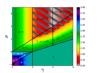
Figure 1: (Color online.) Scaling of mean time to reach fixation with population size. Shading represents the value of exponent $\nu$ where $T\propto N^{\nu}$. The labels give expressions for $\nu$ in each region, with black lines marking boundaries between regions. The diagonal hatches cover the region in which the approximations used are not expected to be accurate.

Suppose however that the degree distribution obeys a power law. In different regions of the $\gamma-\sigma$ plane different moments appearing in (22) diverge with $N$. By carefully examining the ratios between subsequent terms in the series, which involve ratios of moments $\mu_{(k+1)\sigma+k}/\mu_{k\sigma+k-1}$, we can establish that in every region the first term dominates. This then leaves us with

$$r\approx\frac{4\mu_{\sigma+1}\mu_{2\sigma+1}}{N^{2}\mu_{1}\mu_{\sigma}^{2}[2\mu_{\sigma+1}+\mu_{1}A^{-1}]}\;.$$ (23)

The scaling with respect to $N$ depends on whether any or which combination of the moments $\mu_{1},\mu_{\sigma},\mu_{\sigma+1},\mu_{2\sigma+1}$ diverge with $N$ [see Eq. (30)]. This divides the $\sigma$–$\gamma$ plane into a number of regions, as seen in Fig. 1. The mean fixation time is proportional to $1/r$, so finding the population size dependence of Eq. (23) immediately gives us the scaling of $T$ with $N$. In general $T\propto N^{\nu}$, and we give expressions for $\nu$ in the various regions in Fig. 1. We see that in a large area, $\nu=2$ as in the standard case of $H_{ij}$ all equal. For $\gamma<3$ and $\sigma<0$ the mean time to fixation may grow faster than $N^{2}$. On the other hand, for $\sigma>0$ and above the line $\sigma=\gamma-1$, $T$ may grow more slowly than $N^{2}$, with the slowest growth rate $T\propto N^{1/2}$ being achieved when $\gamma=3$ for $\sigma\geq 2$ (though, as we will see, our approximations start to break down when $\nu<1$).

In principle one could also consider further variations, such as $\alpha_{i}$ which are inversely proportional to degree (as in the voter model, or the uniform listening scenario) and so on. These we investigate primarily through numerical simulations, as described below.

IV Numerical calculations of mean fixation time

To check these calculations, and to explore the robustness of our results when assumptions we have made are relaxed, we performed Monte Carlo simulations of the stochastic algorithm described in Sec. II. Explicitly, in each update, we selected a pair of speakers $i$ and $j$ from the distribution $G_{ij}$, generated an utterance $\zeta$ for each speaker, and then applied the update rule (1) to both speakers. This update was repeated until a state of fixation was reached; the mean time to reach fixation is then obtained by averaging over multiple runs. Unless otherwise stated, we used homogeneous initial conditions, that is, all $x_{i}(0)$ are initially set to the same value $x_{0}$.

IV.1 Check of analytical results

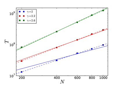
Figure 2: Mean fixation time as a function of population size for $H_{ij}$ independent of degree, as described in Sec. III.1. Results are for a fully connected network with $\beta_{i}$ following a power-law distribution with decay exponent $\gamma=2.0,2.2,2.6$ and constant $\alpha_{i}$. Markers are average fixation times for 5000 numerical runs. Solid lines are expected scaling as given by Eq. (20), dashed lines are best fit curves of the form $T=AN^{\zeta}$.

We first performed numerical simulations of the situations described in Secs. III.1 and III.2 to check our results. We set $H_{ij}=\alpha_{i}\beta_{j}$, and held the $\alpha_{i}$ values constant. For the results shown in Fig. 2 we considered a fully connected network of speakers, that is, each speaker is equally likely to speak with each of the other speakers, and chose the $\beta_{j}$ from a power-law distribution for various values of the power-law exponent $\gamma$.

We found that the agreement with the predictions of Eq. (20) was very good so long as the predicted exponent of growth of $T$ with $N$ was greater than $1$, that is for $\gamma>2$. This includes the region $2<\gamma<3$, in which the mean fixation time, $T$, grows more slowly with $N$ than in the usual situation where $T\propto N^{2}$. That is, the mean time to fixation may be reduced without recourse to any special network structure, merely by allowing heterogeneity in the response of speakers to the utterances of their interlocutors.

For $\gamma\leq 2$, Eq. (20) predicts $T\propto N$. As we we approach this region, we find the theoretical predictions break down. This can be seen in the lowest set of data in the figure. This is not unexpected, if we consider the approximations made to derive our estimates of the mean fixation time. We have assumed that there is a short relaxation period after which the dynamics can be well described by considering only the collective variable $\xi$ (see Blythe (2010) for details). Our calculated fixation times are only for this second stage. Typically the initial relaxation happens in a time of order $N$. We see that if the calculated fixation time is of a similar time scale, the initial relaxation can no longer be ignored. This is the case whenever $\nu$ approaches $1$ when $T\propto N^{\nu}$.

Similar results were obtained for a sparse interaction network in which each speaker had approximately an equal number of neighbors. Thus shortened fixation times are not a consequence of all agents being able to interact with all other agents.

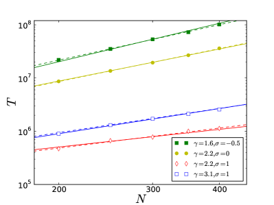
Figure 3: Mean fixation time as a function of population size with $\beta_{i}$ depending on speaker degree, as described in Section III.2. Results are for an random network whose degree distribution obeys a power law $p(k)\propto k^{-\gamma}$. The interaction weights depend on degree through $\beta_{i}\sim k_{i}^{\sigma}$. Markers are average fixation times for 5000 numerical runs. Solid lines are expected scaling as given by Eq. (23) and Fig. 1, dashed lines are best fit curves of the form $T=AN^{\zeta}$.

In Fig. 3 we present simulation results for the situation in which $\beta_{i}$ does depend on the speaker degree. Specifically, speakers were placed on an uncorrelated random network whose degree distribution follows a power law with exponent $\gamma$. These networks were generated using the modified configuration model described in Catanzaro et al. (2005). We then set $\beta_{i}=k_{i}^{\sigma}$. The results shown are for various locations in the $\gamma$–$\sigma$ plane (see Fig. 1). The mean fixation time grows with population size as $T\propto N^{\nu}$ with the value of $\nu$ depending on the parameters $\gamma$ and $\sigma$. The numerical results are in excellent agreement with the $\nu$ values predicted by Eq. (23) for values both smaller and larger than the baseline value of $2$. As before, we found that the agreement fails when the predicted value of $\zeta$ is $1$ or less. This occurs in the region marked with diagonal hatching in Fig. 1.

IV.2 Robustness of the analytical results

We now discuss cases where the conditions for our analytical results, Eqs. (20) and (23) do not hold, but we see nevertheless somewhat similar behavior.

First we investigated the effects of fixed $\beta_{i}$ and heterogeneous $\alpha_{i}$ (on a homogeneous network). By examining Eq. (14) in this case, we see that it is the smallest values of $\alpha_{i}$ which contribute most to $r$. In fact we find that $r\sim\langle 1/\alpha\rangle/N^{2}$. This result is similar to that found in Masuda et al. (2010); Baxter (2011) where different agents in the network could change state with different rates: this is one way to interpret variation of the $\alpha$ parameter in the present work.

In this context, we considered a power-law distribution of values, such that $P(\alpha)\propto\alpha^{-\gamma}$. The moment $\langle 1/\alpha\rangle$ is independent of $\gamma$ in this case [see Eq. (28)], so we would expect to find $T\propto N^{2}$. Indeed this is exactly what we observe through numerical simulations, with the mean fixation time growing as $N^{2}$, exactly as in the standard case, regardless of the value of $\gamma$.

Considering the fact that the smallest $\alpha$ values make the largest contribution, we also carried out simulations with an ‘inverted’ power-law distribution, $P(1/\alpha)\propto(1/\alpha)^{-\gamma}$, that is $P(\alpha)\propto\alpha^{+\gamma}$ with an imposed upper bound instead of a lower bound. In this case we do see mean fixation times changing with $\gamma$, but rather than fixation being sped up, it is slowed down. We find $T\propto N^{\nu}$, with $\nu$ approaching the baseline value of $2$ when $\gamma=3$, and increasing as $\gamma$ decreases, as shown in Fig. 4. Here we do find a difference relative to other cases we investigated, in that the density of the graph also has an effect on the exponent $\nu$: it grows more quickly with decreasing $\gamma$ on a sparse network than a fully connected network.

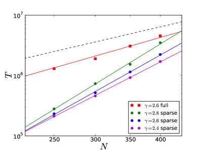
Figure 4: Numerical results for mean fixation time for $\alpha_{i}$ distributed according to inverted power law distributions, with values of $\gamma$ given in the legend. Top line (squares, red online) is for a fully connected graph with $\gamma=2.6$. Lower lines (circles) are for a sparse graph with mean degree $10$ and $\gamma=2.8,2.6,2.4$ from top to bottom. Lines are fitted functions of the form $T=aN^{\xi}$. Dashed line is $aN^{2}$ for comparison.

Returning to heterogeneous $\beta_{i}$ values, we investigated the effect of correlations between the $\beta_{i}$ values of neighboring speakers. To do this, we placed the speakers on a random sparse network, in which each speaker has approximately the same number of neighbors. A list of power law distributed $\beta$ values was created, and the largest value assigned to a randomly chosen speaker. The next largest $\beta$ values were then assigned to the neighbors of this speaker, followed by remaining second-neighbors and so on until all $\beta$ values were assigned. We found that these correlations only slightly affected the scaling of mean fixation time with population size $N$, with $T$ growing as $N^{\nu}$ with exponent $\nu$ similar to that found in Section III.1 for the same $\gamma$. To confirm this result, we repeated the simulations now assigning $\beta$ values from lowest to highest, and considered anticorrelations, in which the lowest $\beta$ values were located on the neighbors of the highest value and so on. In each case the growth of $T$ with $N$ was similar, though the overall prefactor was different to that found in Section III.1. Results are plotted in Fig. 5, compare with Fig. 3. This weak dependence of fixation times on correlations mirrors results found for the voter model on heterogeneous networks Sood and Redner (2005).

Finally we introduced inhomogeneity in the initial conditions. After randomly assigning $\beta_{i}$ values exactly as in Sec. III.1, speakers with the largest $\beta_{i}$’s had their initial grammar value $x_{i}(0)$ set to $1$, while the remainder were set to $0$, such that the overall mean grammar was $x_{0}$. Our calculation assumes the largest contribution to mean fixation time comes from the period after the initial relaxation to a quasi-stationary state, so the initial conditions would not be expected to affect the scaling of mean fixation time with $N$. This was indeed found to be the case, with $T$ scaling with $N$ exactly as found in Sec. III.1. The mean fixation time is affected by initial conditions through the center-of-mass parameter $\xi(0)$ which appears in Eq. (8). This affects the prefactor but not the scaling of $T$ with $N$. We found that $\xi(0)$ differed from the homogeneous case value $x_{0}$, as evidenced by a much greater probability of fixation to state $1$.

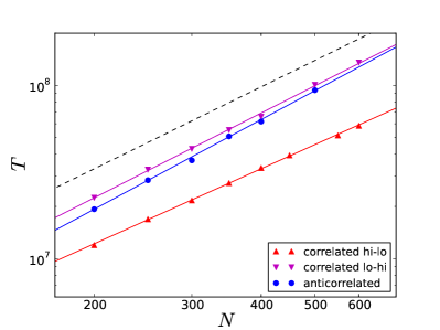
Figure 5: Numerical results for mean fixation time for correlated $\beta_{i}$. Speakers are located on a sparse network and $\beta_{i}$ values distributed according to a power law with exponent $\gamma=2.4$, and correlated (see text) from highest to lowest (triangles), from lowest to highest (inverted triangles) and anti-correlated (circles). Lines are fitted functions of the form $T=aN^{\xi}$, with $\xi=1.44,1.63,1.72$ respectively. For comparison the black dashed line has $\xi=1.57$ which is the slope expected for uncorrelated $\beta_{i}$.

These last numerical investigations thus support the value of the simpler cases for which we made analytic predictions. We find that they give a good indication of the general conditions for finding fixation times shorter than the standard $T\propto N^{2}$.

V Discussion

In this work, we have investigated how asymmetry in the interactions between speakers in a model of language change affects the time to reach a state of fixation (all speakers using a common conventional variant). Although we have couched our discussion in terms of the utterance selection model for language change Baxter et al. (2006), it is worth recalling that the Fokker-Planck equation that describes the continuous-time limit of the dynamics, Eq. (2), also applies to the Wright-Fisher model for changes in gene frequencies in a structured population Crow and Kimura (1970), to Hubbell’s model of ecological community dynamics Hubbell (2001) and, in a limit where all $m_{ij}\to 0$, to a spatially-structured voter model Blythe (2010). Thus our results apply quite generally to models in which the state of a node on a network evolves by copying the state of a neighboring node, whether through a birth-death process (as in the Wright-Fisher or Hubbell model) or by one agent adopting another agent’s behavior (as in the voter and utterance selection models).

As we noted in the introduction, an appealing and useful property of the utterance selection model is that there is a clean and natural separation between the symmetric and asymmetric components of the agent interactions. It is assumed that agents’ linguistic behavior is primarily affected by face-to-face interactions between speakers. Thus whenever agent $i$ is interacting with agent $j$, agent $j$ is interacting with agent $i$. This is reflected in the symmetry of the matrix $G$, viz, $G_{ij}=G_{ji}$. However it is not necessarily the case that the outcome of the interaction is the same for both speakers: agent $i$ may be influenced to a greater degree by agent $j$ than the other way round. In this instance $H_{ij}>H_{ji}$, which results in an asymmetric $H$ matrix .

This formulation has allowed us to explore in a systematic way the consequences of asymmetry in the dynamics by manipulating the $H$ matrix while leaving the $G$ matrix unchanged. This is much harder to do in the context of the voter model (for example), in which the asymmetry is implicit in the model dynamics, rather than specified explicitly as here. Whilst various attempts have been made to separate these two contributions within the context of the voter model, see e.g. Schneider-Mizell and Sander (2009); Moretti et al. (2012), the network structure and asymmetry effects have generally remained entangled to some degree when using the voter model as a starting point.

Our main finding is that the mean time to fixation can be dramatically affected by the presence of large disparities in the influence of different agents, for example, when the $H_{ij}$ are constructed to be drawn from a power-law distribution. We emphasize the distinction with similar results for the voter model on heterogeneous networks (e.g., Sood and Redner (2005); Suchecki et al. (2005a, b); Sood et al. (2008)), in which variation in the degree of each node (combined with the implicit asymmetry of the voter model dynamics) is responsible for such effects. Here we find that the fixation time can be reduced relative to the case of uniform influence ($H_{ij}={\rm const}$) even on homogeneous networks. This result contrasts with those of Masuda et al. (2010); Baxter (2011), in which variation in the willingness to change state (our $\alpha$ parameter) causes a slower onset of fixation, a result we also obtained here.

The specific networks we examined were fully-connected network and sparsely-connected random graphs. We have found that, as in earlier work Baxter et al. (2008), analytical predictions hold when there is a separation of timescales between an initial relaxation and the longer diffusive process that brings the system to fixation. A formal criterion for this separation of timescales is given in Blythe (2010), but in practice we have found the diffusive timescale dominates when it grows more rapidly than linearly with the size of the network $N$. We note that this separation of timescales is in fact seen on the two-dimensional square lattice (although the diffusive timescale is only a factor $\ln N$ longer than the relaxation timescale, Cox (1989)). It is therefore likely that our results hold for the very large class of networks that satisfy the ‘small-world’ property, that is, where the longest distance between any pair of nodes is much smaller than the network size $N$, not just the random graphs that we considered here Newman (2010).

We also found that a wide variety of scaling relationships between the mean fixation time and network size are possible when node influence and degree (a measure of ‘popularity’) co-vary. Here we found cases where fixation may be accelerated or decelerated relative to the baseline case of uniform influence, depending on how influence and degree are correlated. Our results are summarized in the phase diagram of Fig. 1, and are similar in spirit to those obtained in the specific context of the voter model on heterogeneous networks Schneider-Mizell and Sander (2009); Moretti et al. (2012).

Finally, we find that correlations in influence between neighboring nodes only weakly affects the mean time to fixation. This accords for example with a similar finding for degree correlations for the voter model on heterogeneous networks Sood and Redner (2005); Blythe (2010), in which correlations only appear to affect prefactors in the scaling relation between fixation time and network size, not the scaling exponent. This lack of sensitivity to correlations may be due once again to the ‘small-world’ property: since a variant can reach any node on the network in only a few steps, the question of who is using it may become only a second-order consideration.

Taken together with the many results for random-copying processes of various guises that are to be found in the literature, we have by now a more-or-less complete understanding of the factors that enter into the fixation time in these models. There do however remain some generalizations and extensions that remain to be fully explored. Most notably, we have assumed a fixed network structure: it is clear that this structure may also evolve over time, for example, as relationships are formed and broken between members of a social group. Furthermore, all the manifestations of the model we have discussed share the common and crucial property of neutrality with respect to the different variants. That is, the probability that agent $i$ adopts agent $j$’s behavior is independent of what that behavior actually is: there is no selection in the language of genetics or ecology. While both generalizations have been the subject of considerable study (e.g. Nardini et al. (2008); Vazquez et al. (2008) examine dynamic networks and Cherry and Wakeley (2003) selection in a spatial setting) the role of network structure and interaction asymmetry seems to be less well established in these cases.

Appendix A Moments of Power-law Distributions

In this paper we frequently write results in terms of moments of distributions of network properties. We are often interested in distributions with unusually large values, since these model situations where some of the speakers have atypical characteristics. In this Appendix we collect together results on moments of power-law distributions, which are of this kind, that are used in the main text.

Examples of quantities that we are interested in are: the degree $k_{i}$ of nodes of the network of speakers $G_{ij}$ or the matrix of the weights of utterances $H_{ij}$. These are to be sampled from a given distribution. For generic distributions, the moments are not expected to depend on the sample size $N$. However for ‘heavy-tailed’ distributions, the range of values likely to be taken by the samples grows with $N$, and as a consequence the various moments grow as some power of $N$.

Suppose that the probability distribution of some random variable $q$ takes the form

$$P(q)=Aq^{-\gamma}\mbox{ for }q\geq q_{0}\;,$$ (24)

where $A,\gamma$ and $q_{0}$ are constants. In the limit $N\to\infty$ there will be arbitrary large values of $q$ which are sampled. In this case the range of values of $q$ is unbounded ($q_{0}<q<\infty$) and simple integration gives the normalization constant $A$ as $A=(\gamma-1)q_{0}^{\gamma-1}$ ($\gamma>1$) and the $n^{\rm th}$ moment $\mu_{n}$ as

$$\mu_{n}=\frac{\gamma-1}{\gamma-1-y}q_{0}^{n}\;,$$ (25)

which diverges if $n>\gamma-1$.

In real applications, and in particular in this paper, we are interested in the case where $N$ is finite. In this case we expect that there will be some upper cutoff $q_{\rm max}$ that grows with $N$. The easiest way to extract the scaling of this cutoff with $N$ is to put

$$\int_{q_{\rm max}}^{\infty}q^{-\gamma}\propto\frac{1}{N}\;,$$ (26)

motivated by the requirement that the values of $q$ not seen due to finite sample-size effects will have a cumulative probability of order $1/N$. Performing the integral and rearranging yields $q_{\rm max}\sim N^{1/(\gamma-1)}$ (see e.g. Sood and Redner (2005)). More rigorously, one can compute the distribution of the maximum of $N$ power-law random numbers, which has the Fréchet form

$$P_{N}(q)\sim N(\gamma-1)q^{-\gamma}{\rm e}^{-Nq^{1-\gamma}}$$ (27)

for large $N$ and $q_{0}=1$ (see e.g. Castillo et al. (2005)). Using this distribution, one can now calculate the mean value of the maximum $q$ for a given $N$, which is found to scale in the same way as before, $q_{\rm max}\sim N^{1/(\gamma-1)}$. In the context of networks, however, there is an additional condition, in that we do not wish to have any multiple edges. This yields the upper cutoff $\propto N^{1/2}$ for $\gamma<3$ Boguñá et al. (2004). Setting $q_{\rm max}=aN^{1/\rho}$ with $\rho=2$ for $\gamma\leq 3$ and $\rho=(\gamma-1)$ for $\gamma>3$, leads to

$$\mu_{n}=\frac{\gamma-1}{\gamma-1-n}\frac{[q_{0}^{1-\gamma+n}-a^{1-\gamma+n}N^{(1-\gamma+n)/\rho}]}{[q_{0}^{1-\gamma}-a^{1-\gamma}N^{(1-\gamma)/\rho}]}\;.$$ (28)

If $n<\gamma-1$, the terms in Eq. (28) containing $N$ decay with increasing $N$, leading to a value for the moment (for sufficiently large $N$) close to that found in the case of infinite $N$. On the other hand, when $n>\gamma-1$, but $\gamma>1$, the term in $N$ in the numerator diverges, while that in the denominator vanishes, leaving

$$\mu_{n}\approx\frac{\gamma-1}{n-(\gamma-1)}\frac{a^{1-\gamma+n}N^{(1-\gamma+n)/\rho}}{q_{0}^{1-\gamma}}\;.$$ (29)

In summary, for $\gamma>1$, the $n^{\rm th}$ moment is of order:

$$\mu_{n}\sim\begin{cases}N^{(1-\gamma+n)/2}&n>\gamma-1\qquad\gamma\leq 3\\ N^{(1-\gamma+n)/(\gamma-1)}&n>\gamma-1\qquad\gamma>3\\ q_{0}^{n}\sim 1&n<\gamma-1\;.\end{cases}$$ (30)