Interaction-induced enhancement of $g$-factor in graphene

Abstract

We study the effect of electron interaction on the spin-splitting and the $g$-factor in graphene in perpendicular magnetic field using the Hartree and Hubbard approximations within the Thomas-Fermi model. We found that the $g$-factor is enhanced in comparison to its free electron value $g=2$ and oscillates as a function of the filling factor $\nu$ in the range $2\leq g^{\ast}\lesssim 4$ reaching maxima at even $\nu$ and minima at odd $\nu$. We outline the role of charged impurities in the substrate, which are shown to suppress the oscillations of the $g^{\ast}$-factor. This effect becomes especially pronounced with the increase of the impurity concentration, when the effective $g$-factor becomes independent of the filling factor reaching a value of $g^{\ast}\approx 2.3$. A relation to the recent experiment is discussed.

I Introduction

Graphene being subjected to a perpendicular magnetic field exhibits the unusual quantization of the energy spectrum, which is manifested in a non-equally spaced sequence of the Landau levelsGoerbig . In contrast to conventional two-dimensional electron gas (2DEG) systems, the energy difference between the lowest Landau levels is large enough allowing observation of the quantum Hall plateau even at room temperaturesNovoselov2007 . Another interesting peculiarity of graphene is the existence of the 0’th Landau level located precisely at the Dirac point and equally shared by electrons and holesGoerbig . If the magnetic field is high enough, in addition to the Landau level quantization, the level splitting due to the Zeeman effect takes place. This kind of splitting was clearly observed in the recent experiments even for states lying relatively far from the Dirac point, at the filling factors $\nu=\pm 4.$Zhao The Zeeman splitting is by its nature a one-electron effect, which tells that a particle possessing a spin degree of freedom acquires the additional energy in the magnetic field $B$,

$$V_{Z}^{\sigma}=\sigma g\mu_{B}B,$$ (1)

where $\sigma=\pm\frac{1}{2}$ describes two opposite spin states $\uparrow,\downarrow$; $\mu_{B}$ is the Bohr magneton, $g$ is the free electron Lande factor ($g$-factor); $g=2$ for graphene. However, experimentally observed splitting of the Landau levels can not be solely attributed to the Zeeman effect, as this splitting can also be enhanced by electron-electron interactionAndo1974 . The electron-electron interaction in graphene is especially important at high magnetic fields near $\nu=0$ when a new insulating state emergesZhang2010 . Even though the nature of this state is still under debate, it is commonly believed that it is related to the electron-electron interactionZhao .

The enhancement of the spin-splitting due the electron-electron interaction can be described by introducing a phenomenological effective $g$-factor, $g^{\ast},$ which effectively incorporates the interaction effects within the one-electron description. Calculation of the effective $g$-factor was originally done for conventional 2DEG systems based on Si MOSAndo1974 and GaAs/AlGaAsEnglert1982 structures. It was show that the $g$-factor can be enhanced by the electron-electron interaction up to one order of magnitude in comparison to its bare valueEnglert1982 and oscillates as a function of a carrier densityAndo1974 ; Englert1982 . Interaction induced spin-splitting was extensively studied in confined 2DEG structures such as quantum wires Kinaret ; Dempsey ; Tokura ; takis2002 ; Stoof ; Ihnatsenka_wire1 ; Ihnatsenka_wire_comp_strips ; IhnatsenkaCEOQW ; IhnatsenkaMarcus . It was also argued that interaction-induced spontaneous spin-splitting can take place in 2DEG systems even in the absence of magnetic fieldGhosh ; Goni ; Evaldsson .

The enhancement of the effective $g$-factor was also observed in carbon based systems. In graphite the effective $g$-factor is reported to be $g^{\ast}\approx 2.5.$Schneider Recently, Kurganova et. al.kurganova performed measurements of the effective $g$-factor in graphene. It was found to be $g^{\ast}=2.7\pm 0.2$, which is larger than its non-interacting value $g=2$. This indicates that electron-electron interaction effects play an important role and should be taken into account for explanation of the enhanced spin-splitting. Motivated by this experiment we use the Thomas-Fermi approach to study the spin-splitting in realistic two-dimensional graphene sheets in perpendicular magnetic field situated on a dielectric surface and subjected to a smooth confining potential due to charged impurities. (Note that the enhancement of effective $g$-factor in ideal graphene nanoribbons has been recently studied by Ihnatsenka et. alIhnatsenka2012 ). The paper is organized as follows. Sec. II presents the model, where we specify the system at hand and define the Hamiltonian. In Sec. III we discussed the obtained results and provide an explanation for the observed behavior of $g^{\ast}$-factor. Sec. IV contains the conclusions.

II Model

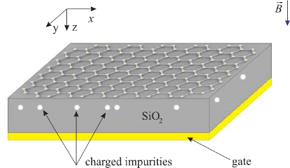
Figure 1: (Color online) Schematic illustration of the studied structure. A graphene sheet is located on an insulating substrate of the width $d$ separating it from a metallic gate. The substrate is contaminated by charged impurities with $q=\pm 1$ situated at the distanace $h=1$ nm apart from the graphene layer.

We consider a system depicted in Fig. 1, consisting of a graphene sheet located on an insulating substrate of the width $d$ with the dielectric constant $\epsilon_{r}.$ (We choose $\epsilon_{r}=3.9$ corresponding to SiO₂). A metallic back gate is used to tune the carrier density by varying the gate voltage $V_{g}$. We assume the charged impurities with the concentration $n_{i}$ are randomly distributed in the substrate at the distance $h=1$ nm apart from the graphene layerdassarma . The whole system is subjected to the perpendicular magnetic field $B$. In order to find the ground-state carrier density, we use the Thomas-Fermi approximation with the local relationGerthards1994 ; Gerthards1997 ; Hannes

$$n_{\sigma}(\mathbf{r})=\left\{\begin{array}[]{ll}\int\limits_{V^{\sigma}(\mathbf{r})}^{\infty}\rho^{\sigma}(E-V^{\sigma}(\mathbf{r}))f_{FD}^{e}(E-E_{F})dE&\text{(electrons)}\\ &\\ \int\limits_{-\infty}^{V^{\sigma}(\mathbf{r})}\rho^{\sigma}(E-V^{\sigma}(\mathbf{r}))f_{FD}^{h}(E-E_{F})dE&\text{(holes)}\\ &\end{array}\right.$$ (2)

between the spin-dependent carrier density $n_{\sigma}(\mathbf{r})$ of the graphene and the total potential energy $V^{\sigma}(\mathbf{r})$. Here $f_{FD}^{e}(E-E_{F})=1/\left(\exp\left(\frac{E-E_{F}}{k_{B}T}\right)+1\right)$ and $f_{FD}^{h}(E,\mu)=1-$ $f_{FD}^{e}(E-E_{F})$ are the Fermi-Dirac distribution functions for electrons and holes respectively, $E_{F}=eV_{g}$ is the Fermi energy. The Landau density of state in graphene is given byGoerbig

$$\rho^{\sigma}(E)=\left\{\begin{array}[]{ll}\sum\limits_{i=0}^{\infty}\frac{g_{\nu}}{2\pi l_{B}^{2}}\delta(E-\hbar\omega_{c}\sqrt{i})&\text{(electrons)}\\ &\\ \sum\limits_{i=0}^{\infty}\frac{g_{\nu}}{2\pi l_{B}^{2}}\delta(E+\hbar\omega_{c}\sqrt{i})&\text{(holes),}\\ &\end{array}\right.$$ (3)

where $\omega_{c}=\sqrt{2}v_{F}/l_{B}$ is the cyclotron frequency, $l_{B}=\sqrt{\hbar/eB}$ is the magnetic length, $v_{F}$ is the Fermi velocity in graphene; the factor $g_{v}=2$ takes into account the valley degeneracy for all levels except of the zeroth one. The zeroth Landau level belongs both to electrons and holes which we take into account by setting $g_{v}=1$. According to Eq. (2), the carrier density $n_{\sigma}(\mathbf{r})$ at the position $\mathbf{r}$ depends on the total potential only at that position.

The total potential

$$V^{\sigma}(\mathbf{r})=V_{H}(\mathbf{r})+V_{U}^{\sigma}(\mathbf{r})+V_{Z}^{\sigma}+V_{imp}(\mathbf{r})$$ (4)

is a sum of the Hartree, Hubbard, Zeeman and the external potential produced by the impurities. The Hartree potential is given byShylau_Cap ; FR ,

$$V_{H}(\mathbf{r})=\frac{e^{2}}{4\pi\epsilon_{0}\epsilon_{r}}\sum_{\mathbf{r}^{{}^{\prime}}\neq\mathbf{r}}n(\mathbf{r}^{\prime})\left(\frac{1}{|\mathbf{r}-\mathbf{r}^{\prime}|}-\frac{1}{\sqrt{|\mathbf{r}-\mathbf{r}^{\prime}|^{2}+4d^{2}}}\right),$$ (5)

where $n(\mathbf{r})=n_{\uparrow}(\mathbf{r})+n_{\downarrow}(\mathbf{r})$ is the local carrier density, and the second term describes a contribution from the mirror chargesHartree . The second term in Eq. (4) is the standard Hubbard potential which is shown to describe carbon electron systems in a good agreement with the first-principles calculationsFR ; Wehling

$$V_{U}^{\sigma}(\mathbf{r})=Un^{\sigma^{\prime}}(\mathbf{r})S_{a},$$ (6)

where $U$ is the effective Hubbard constant and $S_{a}=\frac{3\sqrt{3}}{4}a^{2}$ is the area of unit cell of graphene($a\approx 0.142$ nm is the carbon-carbon distance). In our work we use $U=9.3$ eV which has been recently calculated within the constrained random phase approximationWehling . The third term Eq. (4) is the Zeeman energy given by Eq. (1). The last term in Eq. (4) corresponds to the potential due to charged impurities and is given by

$$V_{imp}(\mathbf{r})=\frac{e^{2}}{4\pi\epsilon_{0}\epsilon_{r}}\times$$

$$\times\sum_{i=1}^{N_{imp}}\left(\frac{q_{i}}{|\mathbf{r}-\mathbf{r}_{i}|^{2}+h^{2}}-\frac{q_{i}}{\sqrt{|\mathbf{r}-\mathbf{r}_{i}|^{2}+(2d-h)^{2}}}\right),$$

where the summation is performed over charged impurities in the dielectric; $\mathbf{r}_{i}$ is the coordinate in the graphene plane of the projection of the $i$-th impurity of the charge $q_{i}$ situated at the distance $h$ from the plane. Equations (2) and (4) are solved self-consistently until a convergence is achieved.

We define the effective $g$-factor as follows,

$$g^{\ast}\mu_{B}B=\left\langle V^{\uparrow}(\mathbf{r})-V^{\downarrow}(\mathbf{r})\right\rangle,$$ (8)

which assumes that spin-splitting in the system is caused by the Zeeman term, Eq. (1), where the free electron value $g$ is replaced by the effective $g$-factor, $g^{\ast}.$ (If the Hubbard interaction is absent, $U=0$, then apparently $g^{\ast}=g)$. Substituting Eq.(4) into Eq.(8), we arrived at the equation used to calculate $g^{\ast},$

$$g^{\ast}=g+\frac{U}{\mu_{B}B}\left\langle n_{\downarrow}(\mathbf{r})-n_{\uparrow}(\mathbf{r})\right\rangle,$$ (9)

where $\langle\ldots\rangle$ denotes spatial averaging over the graphene lattice sites.

III Results and discussion

Figure 2 presents the central result of the paper. It shows the effective $g$-factor as a function of the filling factor $\nu=\frac{n}{n_{B}}$ ($n_{B}=\frac{1}{\pi l_{B}^{2}}$, note that our definition of $n_{B}$ includes a factor of 2 accounting for the valley degeneracy) calculated for different concentrations of impurities.

Figure 2: (Color online) The effective $g$-factor as a function of the filling factor $\nu$ for different concentrations of charged impurities, $n_{i}=0\%,0.02\%,0.08\%,0.2\%$, at the constant perpendicular magnetic field $B=35$T. Inset: the dependence of $g^{\ast}$ on the Hubbard constant $U$ for the fixed $\nu=2.5$. All the calculations are done at the temperature $T=4$ K.

The dependence $g^{\ast}=g^{\ast}(\nu)$ exhibits two main features. First, the effective $g$-factor is enhanced ($g^{\ast}>g$) and oscillates in the range $2\leq g^{\ast}\lesssim 4$ achieving its maximal values at even filling factors $\nu=0,2,4,\ldots$, while having the minima at odd filling factors $\nu=1,3,\ldots$. Second, the increase of the impurity concentration suppresses the enhancement as well as the oscillatory behavior of $g^{\ast}$, such that for high $n_{i}$ the effective $g$-factor becomes only weakly dependent on $\nu$ reaching the value $g^{\ast}\approx 2.3.$

Figure 3: (Color online) The dependence of (a) the charge concentration, (b) the polarization and (c) the effective $g$-factor on the filling factor in almost ideal system (i.e. in a graphene sheet with the low concentration of charged impurities in the substrate, $n_{i}=0.02\%$).

In order to understand the observed behavior let us first consider in details the case of a low concentration of impurities shown on Fig. 3, where $g^{\ast}$-factor dependence for $n_{i}=0.02\%$ is complemented by the spin-density and the polarization dependencies. For small $n_{i}$ the effect of impurities is small and the filling factor can be directly related to the number of the occupied Landau levels of an ideal system (i.e. without impurities). For a fixed value of the magnetic field the increase of the filling factor corresponds to the increase of charge density through subsequent population of the Landau levels. As seen in Fig. 3, the total spin polarization $P=\left\langle P(\mathbf{r})\right\rangle=\left\langle\frac{|n_{\downarrow}(\mathbf{r})|-|n_{\uparrow}(\mathbf{r})|}{|n_{\downarrow}(\mathbf{r})|+|n_{\uparrow}(\mathbf{r})|}\right\rangle$ exhibits the same qualitative behavior as the $g$-factor (except for $\nu=0$, which will be discussed below). At $\nu=1$ the $g^{\ast}$-factor reaches its minimal value $g^{\ast}=g$. In this case the Fermi energy is located in between the 0’th Landau level (LL0) and the 1’st Landau level (LL1), i.e. the LL0 is fully occupied, while LL1 is completely empty (see inset in Fig. 3). This gives rise to the equal spin-up and spin-down densities and hence to the zero spin polarization. The increase of the filling factor in the range $1<\nu<2$ leads to gradual population of 1’st spin-down ($\downarrow$) Landau level (LL1($\downarrow$)) and, in turn, to the increase of $n_{\downarrow}$, while $n_{\uparrow}$ does not change. (Note that even though in our model the DOS is given by the delta functions, it is effectively smeared out by a non-zero temperature, which results in a smooth change of the charge densities.) Since the difference $n_{\downarrow}-n_{\uparrow}$ increases, according to Eq. (9) $g^{\ast}$ grows and reaches its maximum $g^{\ast}\approx 3.5$ at $\nu=2$, when the Fermi energy lies in the middle of two spin-split levels corresponding to the same Landau level (LL1). The enhancement of the effective $g$-factor in comparison to its noninteracting value is apparently caused by the Hubbard term in Eq. (4). The Hubbard interaction enhances the spin-splitting triggered by the Zeeman interaction giving rise to $g^{\ast}>g$.

When the filling factor is further increased from $\nu=2$ to $\nu=3$, i.e. the Fermi energy is shifted towards higher energies, the population of the spin-up ($\uparrow$) level belonging to LL1 gradually grows, while the density of the spin-down electrons ($\downarrow$) belonging to the same LL1 remains unchanged as the later level remains completely filled. Eventually, at $\nu=3$ the spin densities become equal, $n_{\downarrow}\approx n_{\uparrow}$, the system is not spin-polarized ($P=0$) and the effective $g$-factor again reaches its minimum $g^{\ast}=g$. The same physics is responsible for similar oscillatory behavior of the effective $g$-factor and the polarization for higher filling factors.

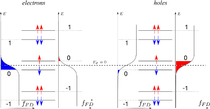
Figure 4: (Color online) Schematic illustration of Landau levels population at $\nu=0$ for electrons and holes. Shaded regions (red and blue) correspond to states occupied in the LL0 by spin-up and spin-down electrons.

The dependencies of the effective $g$-factor and the polarization are qualitatively different for $\nu<1$. Namely, the polarization drops to zero at $\nu=0$, while the effective $g$-factor reaches its maximum, see Fig. 3(b),(c). This is in contrast to all other even filling factors when both $g^{\ast}$ and $P$ exhibit maxima. This can be understood as follows. In contrast to other Landau levels, LL0 is equally shared by electrons and holes at $E_{F}=0$, which is a distinct feature of graphene. As illustrated in Fig. 4, when the magnetic field is high enough, i.e. the spin-split levels are well resolved, electrons predominantly populate the LL0($\downarrow$) state, while LL0($\uparrow$) is mostly occupied by holes. As a result, $n_{\downarrow}=-n_{\uparrow}$, and therefore the effective $g$-factor reaches the maximum because of the Hubbard term $\sim U(n_{\downarrow}-n_{\uparrow})=2Un_{\downarrow}$. On the other hand, at $\nu=0$ the graphene is electrically neutral, $n=n_{\downarrow}+n_{\uparrow}=0$, and spin-polarization is absent, $P=0,$ since $|n_{\downarrow}|=|n_{\uparrow}|$. Note that the effect of electron-electron interaction on spin splitting in graphene nanoribbons at $\nu\approx 0$ was discussed in Ref.[Shylau2011 ].

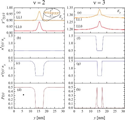
Figure 5: (Color online) Distribution of (a),(e) the self-consistent potential, (b),(f) spin-up and (c),(g) spin-down electron density, (d),(h) the spin polarization for a single impurity at different filing factors $\nu=2$ and $\nu=3$ (left and right columns respectively).

The above analysis is strictly speaking applicable only for ideal graphene, when $n_{i}=0$. In this case, the range of $g$-factor oscillations can be easily estimated from Eq. (9). At odd filling factors, when $n_{\downarrow}=n_{\uparrow}$, Eq. (9) gives $g_{\text{min}}^{\ast}=g=2$. At even filling factors, when $E_{F}$ lies between two spin-split levels of a given Landau level, for the chosen parameters $U$ and $B,$ the effective $g$-factor $g_{\text{max}}^{\ast}=2+\frac{US_{a}}{\pi l_{B}^{2}\mu_{B}}\approx 4$, which is in accordance with our numerical calculations (Fig. 2, $n_{i}=0$). However, in the presence of impurities, this is not the case anymore, as the oscillations of the effective $g$-factor get suppressed and $g^{\ast}$ never reaches $g_{\text{max}}^{\ast}$ and always stays larger than $g_{\text{min}}^{\ast}$, see Fig. 2.

In order to explain the influence of impurities on the $g$-factor, let us now consider a system consisting of a single repulsive impurity only. Figure 5 (a) shows the cross section of the self-consistent potentials $V^{\uparrow}$ and $V^{\downarrow}$ for spin-up and spin-down electrons respectively. The LL0($\downarrow,\uparrow$) coincides with the self-consistent potential $V^{\downarrow,\uparrow}$, while the positions of the LL1($\downarrow,\uparrow$) are given by $V^{\downarrow,\uparrow}+\hbar\omega_{c}$. We have chosen two representative values of the filling factor, namely, $\nu=2$ and $\nu=3$ corresponding to maximum and minimum values of the effective $g$-factor.

At $\nu=2$, which in ideal graphene corresponds to the almost occupied spin-down and almost empty spin-up states of the LL1, $g^{\ast}$ reaches the maximal value. Figure 5 shows that the LL1($\downarrow$) is pinned to the Fermi energy $E_{F}$. (For the effect of pinning of $E_{F}$ within the Landau levels see e.g. Ref. Davies ). The states lying in the interval $|E-E_{F}|<2\pi k_{B}T$ are partially filed $0<f_{FD}<1$ and therefore the electron density can be redistributed under an influence of an external potential. These states represents the compressible stripsChklovskii1992 , which in our case extends over the whole system (except of the impurity region). The presence of negative impurity leads to the distortion of the potential as depicted in Fig. 5(a). As a result, in the impurity region the LL1($\downarrow$) raises above $E_{F}$ and this state becomes depopulated, Fig. 5(c). (Note that LL1($\uparrow$) is practically depopulated even in an absence of the impurity, Fig. 5(b)). As a result, the spin density difference, $n_{\downarrow}-n_{\uparrow},$ decreases in the impurity region, which apparently leads to the decrease of $P$ and $g^{\ast}$ in comparison to ideal graphene, see Fig. 5(d).

On the other hand, the influence of the impurity is opposite for odd $\nu$. At $\nu=3$ the system is predominantly in a unpolarized state, which is manifested by the minimum of $g^{\ast}$. However, the distortion of the potential due to the impurity gives rise to the formation of a compressible strip around the impurity, where $E_{F}$ intersects the LL1. This is clearly seen in Fig. 5 (e) where the compressible strip corresponds to regions where the potential is flat because of the pinning to $E_{F}$ within the energy window $|E-E_{F}|<2\pi k_{B}T$ (where $0<f_{FD}<1).$ Because of the partial filling of the compressible strip, the electron density there can be easily redistributed there. As a result, the Hubbard interaction pushes up and depopulates the LL1($\uparrow$) while the LL1($\downarrow$) remains populated, see Figs. 5(f),(g). This leads to a local spin polarization around the impurity as illustrated in Fig.(5)(h). therefore, the overall polarization is no longer zero, $\langle P(\mathbf{r})\rangle>0$ and, hence, the effective $g$-factor does not drop to the minimum value, remaining $g^{\ast}>g_{\text{min}}^{\ast}$.

Summarizing, the influence of a single impurity is twofold: when the system is predominantly spin-polarized (even $\nu$), the impurity decreases the average polarization and the effective $g$-factor by locally pushing-up the Landau levels and depopulating them; in the opposite case of a predominantly non-polarized system (odd $\nu$), the impurity leads to the local formation of the spin-polarized compressible strips, which instead increases the average polarization and the effective $g$-factor.

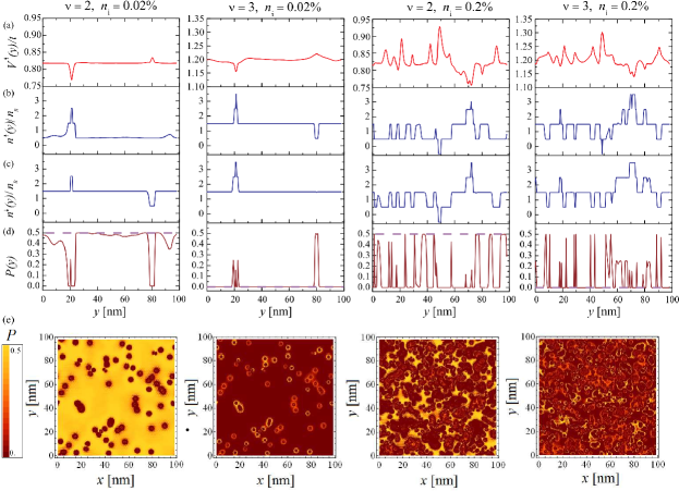
Figure 6: (Color online). The spin resolved potential, densities and polarization for different concentration charged of impurities($n_{i}=0.2\%,0.02\%$) and for different filling factors ($\nu=2,3$). The one-dimensional plots of (a) $V^{\uparrow}(y),$ (b) the spin-up and (c) spin-down charge densities, and (d) the spin polarization $P(y)$ as a functions of $y$ for $x=50$ nm. Dashed lines correspond to the ideal system (without impurities). (e) The 2D plot of the spatially resolved spin polarization $P(x,y)$ in a graphene sheet. The system parameters are $N_{x}=800$, $N_{y}=461$, $d=10$ nm, $B=50$ T.

Having understood the effect of a single impurity on the average polarization and the effective $g$-factor it is straightforward to generalize the obtained results for an arbitrary concentration of impurities. The higher concentration $n_{i}$, the larger influence of impurities on the average value of the spin-polarization and the effective $g$-factor. As a result, an increase of the impurity concentration leads to the suppression of the amplitude of oscillations as shown in Fig. 2.

Note that for a sufficiently large impurity concentration (in our case $n_{i}=0.2\%$), the oscillations of $g^{\ast}$ get practically suppressed and $g^{\ast}$ becomes rather independent on the filling factor, see Fig. 2. This effect can be understood from a comparison of two distinct cases of low and high impurity concentration, $n_{i}=0.02\%$ and $n_{i}=0.2\%$, see Fig. 6. When the impurity concentration is low ($n_{i}=0.02\%$, two left columns in Fig. 6), the self-consistent potentials produced by different impurities do not overlap and the system can be treated as an assembly of independent impurities. (The potential is flat everywhere besides narrow regions close to the impurities, see (a)-panels for $n_{i}=0.02\%$ in Fig. 6). At $\nu=2$ the presence of impurities decreases locally polarization (dips on (c)-panel), while at $\nu=3$ the local polarization increases (peaks on (c)-panel).

However, when the impurity concentration is high ($n_{i}=0.2\%$, two right columns in Fig. 6), the potentials produced by different impurities start to overlap and the analysis in terms of a single impurity is no longer justified. A given value of the filling factor can not be associated with a certain number of the Landau levels, since the potential is strongly distorted in comparison to the ideal case ((a)-panels for $n_{i}=0.2\%$ in Fig. 6) and therefore electrons occupy different Landau levels ((b) and (c)-panels for $n_{i}=0.2\%$ in Fig. 6). In fact, the deviations in the potential and densities from those of the ideal case become so significant, so the difference between the cases of $\nu=2$ and $\nu=3$ is practically washed out (c.f. two right columns in Fig. 6). As a result, the average value of the polarization and the effective $g$-factor becomes practically independent of the filling factor.

In the model used in our calculation the enhancement of the $g$-factor is caused by the Hubbard term in the potential, Eqs. (6) and (9). Let us briefly discuss how the calculated value of $g^{\ast}$ depends on the Hubbard constant $U$. While we used value $U\approx 3.5t$Wehling , the current literature reports various estimations of $U$ in the range $0.5t\lesssim U\lesssim 2t,$Yazyev ; Jung ; Tao where $t\approx 2.7$ eV is the hopping integral in the standard $p$-orbital tight-binding HamiltonianGoerbig . We calculated the dependencies $g^{\ast}=g^{\ast}(\nu)$ for different values of the parameter $U$ and found that the results show the same qualitative behaviour and the calculated value of $g^{\ast}$ scales linearly with $U.$ This is illustrated in the inset to Fig. 2 which shows a dependence of the effective $g$-factor on the Hubbard constant for a representative value of $\nu=2.5.$

Let us now discuss the relation of our findings to the recent experiment. Measurements done by Kurganova et al.kurganova exhibit the enhancement of the effective spin-splitting leading to the effective $g$-factor $g^{\ast}=2.7\pm 0.2$. Also, the enhanced effective $g$-factor was found to be practically independent on $\nu$. Our calculations show that for low impurity concentrations, $g^{\ast}$ exhibits a pronounced oscillatory behavior in the range $2\leq g^{\ast}\lesssim 4,$ and it becomes rather independent of $\nu$ for larger $n_{i}$ reaching a saturated value $g^{\ast}\sim 2.3.$ Our calculations therefore strongly suggest that impurities always present in realistic samples play an essential role in suppressing the oscillatory behavior of $g^{\ast}.$ Note that in real systems the oscillations of $g^{\ast}$ can be smoothed by a number of additional factors. The measurements of Kurganova et. al kurganova were performed in a tilted magnetic fields and at large filling factors $\nu>6$. In this case the distance between the adjacent Landau levels is comparable to the Zeeman splitting which results in stronger overlap of the successive Landau levels and eventually leads to an additional smearing of $g^{\ast}$. Therefore our calculations motivate for further studies of the effective $g$-factor close to $\nu=0$, where the oscillatory behavior of $g^{\ast}$ is expected to be more pronounced. Our finding also indicate that the oscillatory behavior of the effective $g$-factor is expected to be more pronounced in suspended samples where the influence of charged impurities will be much less important.

Finally, it is noteworthy that spin-splitting of in grapheneLundeberg and graphene quantum dotsGuttinger was also experimentally studied in a parallel magnetic filed. It was concluded that in this case the effective $g$-factor does differ from its free-electron value. This can be explained by the fact that in the parallel field the Landau levels do not form and therefore the interaction induced enhancement of the $g^{\ast}$-factor is small.

IV Conclusions

In this work we employed the Thomas-Fermi approximation in order to study the effective $g$-factor in graphene in the presence of a perpendicular magnetic field taking into account the effect of charged impurities in the substrate. We found that electron-electron interaction leads to the enhancement of the spin splitting, which is characterized by the increase of the effective $g$-factor. We showed that for low impurity concentration $g^{\ast}$ oscillates as a function of the filling factor $\nu$ in the range from $g_{\text{min}}^{\ast}=2$ to $g_{\text{max}}^{\ast}\approx 4$ reaching maxima at even filling factors and minima at odd ones. Finally, we outlined the influence of impurities on the spin-splitting and demonstrated that the increase of the impurity concentration leads to the suppression of the oscillation amplitude and to a saturation of the the effective $g$-factor around a value of $g^{\ast}\approx 2.3$.

- (1) M. O. Goerbig, Rev. Mod. Phys. 83, 1193 (2011).
- (2) K. S. Novoselov, Z. Jiang, Y. Zhang, S. V. Morozov, H. L. Stormer, U. Zeitler, J. C. Maan, G. S. Boebinger, P. Kim, and A. K. Geim, Science 315, 1379 (2007).
- (3) Yue Zhao, Paul Cadden-Zimansky, Fereshte Ghahari, and Philip Kim, Phys. Rev. Lett. 108, 106804 (2012).
- (4) T. Ando and Y. Uemura, J. Phys. Soc. Jpn. 37, 1044 (1974).
- (5) L. Zhang, Y. Zhang, M. Khodas, T. Valla, and I. A. Zaliznyak, Phys. Rev. Lett. 105, 046804 (2010).
- (6) T. Englert, D. Tsui, A. Gossard, and C. Uihlein, Surf. Sci. 113, 295 (1982).
- (7) J. M. Kinaret and P. A. Lee, Phys. Rev. B 42, 11768 (1990).
- (8) J. Dempsey, B. Y. Gelfand, and B. I. Halperin, Phys. Rev. Lett. 70, 3639 (1993).
- (9) Y. Tokura and S. Tarucha, Phys. Rev. B 50, 10981 (1994).
- (10) Z. Zhang and P. Vasilopoulos, Phys. Rev. B 66, 205322 (2002).
- (11) T. H. Stoof and G. E. W. Bauer, Phys. Rev. B 52, 12143 (1995).
- (12) S. Ihnatsenka and I. V. Zozoulenko, Phys. Rev. B 73, 075331 (2006).
- (13) S. Ihnatsenka and I. V. Zozoulenko, Phys. Rev. B 73, 155314 (2006).
- (14) S. Ihnatsenka and I. V. Zozoulenko, Phys. Rev. B 74, 075320 (2006).
- (15) S. Ihnatsenka and I. V. Zozoulenko, Phys. Rev. B 78, 035340 (2008).
- (16) A. Ghosh, C. J. B. Ford, M. Pepper, H. E. Beere, and D. A. Ritchie, Phys. Rev. Lett. 92, 116601 (2004).
- (17) A. R. Goñi, P. Giudici, F. A. Reboredo, C. R. Proetto, C. Thomsen, K. Eberl, and M. Hauser, Phys. Rev. B 70, 195331 (2004).
- (18) M. Evaldsson, S. Ihnatsenka, and I. V. Zozoulenko, Phys. Rev. B 77, 165306 (2008).
- (19) J. M. Schneider, N. A. Goncharuk, P. Vasek, P. Svoboda, Z. Vyborny, L. Smrcka, M. Orlita, M. Potemski, and D. K. Maude, Phys. Rev. B 81, 195204 (2010).
- (20) E. V. Kurganova, H. J. van Elferen, A. McCollam, L. A. Ponomarenko, K. S. Novoselov, A. Veligura, B. J. van Wees, J. C. Maan, and U. Zeitler, Phys. Rev. B, 84, 121407, (2011).
- (21) S. Ihnatsenka and I. V. Zozoulenko, arXiv:1206.6251v1 [cond-mat.mes-hall] (2012).
- (22) Enrico Rossi and S. Das Sarma, Phys. Rev. Lett. 101, 166803 (2008).
- (23) K. Lier and R. R. Gerhardts, Phys. Rev. B 50, 7757 (1994).
- (24) J. H. Oh and R. R. Gerhardts, Phys. Rev. B 56, 13519 (1997).
- (25) W.-R. Hannes, M. Jonson and M. Titov, Phys. Rev. B 84, 045414 (2011).
- (26) A. A. Shylau, J. W. Klos, and I. V. Zozoulenko, Phys. Rev. B 80, 205402 (2009).
- (27) J. Fernández-Rossier, J. J. Palacios, and L. Brey, Phys. Rev. B 75, 205441 (2007).
- (28) To facilitate calculations of the summation in Eq.(5) was performed numerically in the region . Outside this region the charge density was assumed to be uniform , such that that the additional potential produced by by charges in the this region was evaluated analytically.
- (29) T. O. Wehling, E. Şaşioğlu, C. Friedrich, A. I. Lichtenstein, M. I. Katsnelson and S. Blügel, Phys. Rev. Lett. 106, 236805 (2011).
- (30) A. A. Shylau and I. V. Zozoulenko, Phys. Rev. B 84, 075407 (2011).
- (31) J. H. Davies, The physics of low-dimensional semiconductors: an introduction, (Cambridge university press, Cambridge, 1998).
- (32) D. B. Chklovskii, B. I. Shklovskii, and L. I. Glazman, Phys. Rev. B 46, 4026 (1992).
- (33) O. V. Yazyev, Phys. Rev. Lett. 101, 037203 (2008).
- (34) J. Jung and A. H. MacDonald, Phys. Rev. B 80, 235417 (2009).
- (35) C. Tao, L. Jiao, O. V. Yazyev, Y.-C. Chen, J. Feng, X. Zhang, R. B. Capaz, J. M. Tour, A. Zettl, S. G. Louie, H. Dai, and M. F. Crommie, Nat. Phys. 7, 616 (2011).
- (36) Mark B. Lundeberg and Joshua A. Folk, Nat. Phys. 5, 894 (2009)
- (37) J. Guttinger, T. Frey, C. Stampfer, T. Ihn, and K. Ensslin, Phys. Rev. Lett. 105, 116801 (2010).