Nonuniformity effects in the negative effective magnetic pressure instability

Abstract

Using direct numerical simulations (DNS) and mean-field simulations (MFS), the effects of non-uniformity of the magnetic field on the suppression of the turbulent pressure is investigated. This suppression of turbulent pressure can lead to an instability which, in turn, makes the mean magnetic field even more non-uniform. This large-scale instability is caused by a resulting negative contribution of small-scale turbulence to the effective (mean-field) magnetic pressure. We show that enhanced mean current density increases the suppression of the turbulent pressure. The instability leads to magnetic flux concentrations in which the normalized effective mean-field pressure is reduced to a certain value at all depths within a structure.

1 Introduction

The Sun’s magnetic field is generally believed to be due to a turbulent dynamo operating in the convection zone in its outer 30% by radius [19, 21, 22, 26, 2]. Recent simulations performed by a number of groups have shown that the magnetic field is produced in the bulk of the convection zone. According to the flux tube scenario, most of the toroidal magnetic field resides at the bottom of the convection zone, or possibly just beneath it [7, 23]. Another possibility is that most of the toroidal field resides in the bulk of the convection zone, but that its spatio-temporal properties are strongly affected by the near-surface dynamics [8], or the near-surface shear layer [1]. In any case, the question then emerges how one can explain the formation of active regions out of which sunspots develop during the lifetime of an active region.

In the past, this question was conveniently bypassed by referring to the possible presence of a strong toroidal flux belt at the bottom of the convection zone, where they would be in a stable state, except that every now and then they would become unstable, for example to the clamshell or tipping instabilities [6]. However, if the magnetic field is continuously being destroyed and regenerated by the turbulence in the convection zone proper, the mechanism for producing active regions and eventually sunspots must be one that is able to operate within a turbulent environment. One such mechanism may be the negative effective magnetic pressure instability (NEMPI) which is based on the suppression of turbulent pressure by a weak mean magnetic field, leading therefore to a negative effective (or mean-field) magnetic pressure and, under suitable conditions, to an instability [14, 15, 18, 17, 24]. This has been the subject of intensive research in recent years [3, 5, 10, 11, 12, 9, 20], following the first detection of such an instability in direct numerical simulations [DNS; see 4]. Another mechanism that has been discussed in connection with the production of magnetic flux concentrations is related to the suppression of the turbulent convective heat flux [13]. Meanwhile, simulations of realistic solar convection have demonstrated that large-scale magnetic flux inhomogeneities can develop when horizontal magnetic flux is injected at the bottom of the simulation domain [25], but it remains to be seen whether this is connected with any of the two aforementioned mechanisms.

The purpose of the present paper is to investigate the possibility that higher-order contributions (involving higher spatial derivatives of the mean magnetic field) might play a role in NEMPI. We do this by using DNS to measure the resulting turbulent transport coefficients in cases where a measurable mean current density develops in the DNS. Note that even for an initially uniform mean magnetic field, a mean current density develops as a consequence of NEMPI itself, which redistributes an initially uniform magnetic field into a structured one. To investigate this process further, we use appropriately tailored mean-field simulations (MFS) that show how the spatial variations of the negative effective magnetic pressure vary in space as the instability runs further into saturation. We begin by discussing first the basic equations and turn then to the results. Throughout this work we use an isothermal equation of state which yields the simplest possible system to investigate this process.

2 Basic equations

In this paper we use both DNS and MFS to study the effects of nonuniformity of the magnetic field of the development of NEMPI. In the DNS, the solutions turn out to have a large-scale two-dimensional pattern which can best be isolated using averaging over the $y$ direction. Furthermore, by imposing a uniform magnetic field, we can determine some of the turbulent transport coefficients that characterize the dependence of the Reynolds and Maxwell stress on the mean field. This is generally done by determining the total mean stress

$$\overline{\Pi}_{ij}=\overline{\rho}\,\overline{U_{i}U_{j}}+{\textstyle{1\over 2}}\delta_{ij}\overline{\mbox{\boldmath$B$}{}^{2}}-\overline{B_{i}B_{j}}.$$ (1)

Here, the vacuum permeability is set to unity and overbars indicate $y$ averages. This total mean stress has contributions from the fluctuations,

$$\overline{\Pi}_{ij}^{\rm f}=\overline{\rho}\,\overline{u_{i}u_{j}}+{\textstyle{1\over 2}}\delta_{ij}\overline{\mbox{\boldmath$b$}{}^{2}}-\overline{b_{i}b_{j}},$$ (2)

where $\mbox{\boldmath$u$}{}=\mbox{\boldmath$U$}{}-\overline{\mbox{\boldmath$U$}}{}$ and $\mbox{\boldmath$b$}{}=\mbox{\boldmath$B$}{}-\overline{\mbox{\boldmath$B$}}{}$ are the departures from the averaged fields. Here $\overline{\mbox{\boldmath$U$}}{}$ and $\overline{\mbox{\boldmath$B$}}{}$ are the mean velocity and magnetic fields, and $\overline{p}$ is the mean fluid pressure. This, together with the contribution from the mean field, namely

$$\overline{\Pi}_{ij}^{\rm m}=\overline{\rho}\,\overline{U}_{i}\overline{U}_{j}+\delta_{ij}\left(\overline{p}+{\textstyle{1\over 2}}\overline{\mbox{\boldmath$B$}}{}^{2}\right)-\overline{B}_{i}\overline{B}_{j}-2\nu\overline{\rho}\,\overline{\sf S}_{ij},$$ (3)

yields the total mean stress tensor, i.e., $\overline{\Pi}_{ij}=\overline{\Pi}_{ij}^{\rm m}+\overline{\Pi}_{ij}^{\rm f}$. The term $\overline{\Pi}_{ij}^{\rm m}$ depends only on the mean field and is therefore directly obtained in MFS, while $\overline{\Pi}_{ij}^{\rm f}$ is caused by the fluctuating velocity and magnetic fields and requires a parameterization. It has a contribution independent of the mean field, $\overline{\Pi}^{\rm f,0}_{ij}$, and one that depends on it, $\Delta\overline{\Pi}_{ij}^{\rm f}(\overline{B})$. Much of the recent work in this field focussed on the parameterization

$$\Delta\overline{\Pi}_{ij}^{\rm f}=-{\textstyle{1\over 2}}q_{\rm p}(\beta)\,\delta_{ij}\,\overline{\mbox{\boldmath$B$}}{}^{2}+q_{\rm s}(\beta)\,\overline{B}_{i}\overline{B}_{j}+q_{\rm g}(\beta)\,\overline{\mbox{\boldmath$B$}}{}^{2}\hat{g}_{i}\hat{g}_{j},$$ (4)

where $\hat{g}_{i}=g_{i}/g$ is the unit vector in the direction of gravity. This difference in the mean stress, $\Delta\overline{\Pi}_{ij}^{\rm f}(\overline{B})$, is caused solely by the presence of the mean magnetic field $\overline{\mbox{\boldmath$B$}}{}$, where $q_{\rm p}(\beta)$ is found to be a positive function of $\beta=|\overline{\mbox{\boldmath$B$}}{}|/B_{\rm eq}$ only, and, for weak magnetic fields, $q_{\rm p}(\beta)$ is well in excess of unity for $\mbox{\rm Re}_{\rm M}\gg 1$, thus overcoming the magnetic pressure from the mean field itself. However the functions $q_{\rm s}(\beta)$ and $q_{\rm g}(\beta)$ were found to be small for isothermal turbulence. The net result for the sum $\overline{\Pi}_{ij}^{\rm m}+\Delta\overline{\Pi}_{ij}^{\rm f}$ is

$$\overline{\Pi}_{ij}\approx\overline{\Pi}^{\rm f,0}_{ij}+\delta_{ij}\,p_{\rm eff}(\overline{B}/B_{\rm eq})-\overline{B}_{i}\overline{B}_{j},$$ (5)

where $p_{\rm eff}={\textstyle{1\over 2}}\left[1-q_{\rm p}(\beta)\right]\,\overline{\mbox{\boldmath$B$}}{}^{2}$ is the mean effective magnetic pressure that is negative for $\beta<\beta_{\rm crit}$, where $\beta_{\rm crit}\approx 0.5$ (depending on other details of the system). This results in a large-scale instability (NEMPI) and the formation of large-scale inhomogeneous magnetic structures.

In the nonlinear stage of NEMPI, the mean magnetic field becomes strongly nonuniform. This implies that the Maxwell–Reynolds stress tensor $\Delta\overline{\Pi}_{ij}^{\rm f}$ may depend also on spatial derivatives of the mean magnetic field, i.e.,

$$\Delta\overline{\Pi}_{ij}^{\rm f} = -{\textstyle{1\over 2}}\delta_{ij}\,q_{\rm p}\,\overline{\mbox{\boldmath$B$}}{}^{2}+q_{\rm s}\,\overline{B}_{i}\overline{B}_{j}+q_{\rm g}\,\overline{\mbox{\boldmath$B$}}{}^{2}\hat{g}_{i}\hat{g}_{j}+C_{1}\overline{B}_{i,m}\overline{B}_{j,m}$$ (6)

$$+C_{2}\overline{B}_{m,i}\overline{B}_{m,j}+C_{3}\,(\overline{B}_{i,m}\overline{B}_{m,j}+\overline{B}_{j,m}\overline{B}_{m,i}),$$

where $\overline{B}_{i,j}=\nabla_{j}\overline{B}_{i}$. We decompose $\overline{B}_{i,j}$ into symmetric and antisymmetric parts:

$$\overline{B}_{i,j}=(\partial\overline{B})_{ij}-{\textstyle{1\over 2}}\varepsilon_{ijm}\overline{J}_{m},$$ (7)

where $(\partial\overline{B})_{ij}={\textstyle{1\over 2}}(\overline{B}_{i,j}+\overline{B}_{j,i})$. Substituting equation (7) into equation (6) we obtain:

$$\Delta\overline{\Pi}_{ij}^{\rm f} = -{\textstyle{1\over 2}}\delta_{ij}\,q_{\rm p}\,\overline{\mbox{\boldmath$B$}}{}^{2}+q_{\rm s}\,\overline{B}_{i}\overline{B}_{j}+q_{\rm g}\,\overline{\mbox{\boldmath$B$}}{}^{2}\hat{g}_{i}\hat{g}_{j}$$ (8)

$$-q_{\rm J}\,\left(\overline{J}^{2}\delta_{ij}-\overline{J}_{i}\overline{J}_{j}\right)-q_{\rm F}\,(\partial\overline{B})_{im}(\partial\overline{B})_{mj}$$

$$-q_{\rm I}\,\left(\varepsilon_{iml}(\partial\overline{B})_{mj}+\varepsilon_{jml}(\partial\overline{B})_{mi}\right)\overline{J}_{l}.$$

Let us consider a mean magnetic field of the form $\overline{\mbox{\boldmath$B$}}{}=(0,\overline{B}_{y}(x,z),0)$, so $(\partial\overline{B})_{xy}=\overline{J}_{z}/2$, $(\partial\overline{B})_{yz}=-\overline{J}_{x}/2$ and

$$(\partial\overline{B})_{im}(\partial\overline{B})_{mj}={1\over 4}\left(\matrix{\overline{J}_{z}^{2}&0&-\overline{J}_{x}\overline{J}_{z}\cr 0&\overline{J}^{2}&0\cr-\overline{J}_{x}\overline{J}_{z}&0&\overline{J}_{x}^{2}\cr}\right),$$ (9)

$$\left(\varepsilon_{iml}(\partial\overline{B})_{mj}+\varepsilon_{jml}(\partial\overline{B})_{mi}\right)\overline{J}_{l}$$

$$\quad\quad\quad\quad={1\over 2}\left(\matrix{\overline{J}_{z}^{2}&0&-\overline{J}_{x}\overline{J}_{z}\cr 0&-\overline{J}^{2}&0\cr-\overline{J}_{x}\overline{J}_{z}&0&\overline{J}_{x}^{2}\cr}\right).$$ (10)

Equations (8) and (9) yield:

$$\Delta\overline{\Pi}_{xx}^{\rm f} = -\tilde{q}_{\rm J}\,\overline{J}_{z}^{2}-{\textstyle{1\over 2}}q_{\rm p}\,\overline{B}^{2},$$ (11)

$$\Delta\overline{\Pi}_{yy}^{\rm f} = \tilde{q}_{\rm I}\,\overline{J}^{2}+\left(q_{\rm s}-{\textstyle{1\over 2}}q_{\rm p}\right)\,\overline{B}^{2},$$ (12)

$$\Delta\overline{\Pi}_{zz}^{\rm f} = -\tilde{q}_{\rm J}\,\overline{J}_{x}^{2}+\left(q_{\rm g}-{\textstyle{1\over 2}}q_{\rm p}\right)\,\overline{B}^{2},$$ (13)

$$\Delta\overline{\Pi}_{xz}^{\rm f} = \tilde{q}_{\rm J}\,\overline{J}_{x}\,\overline{J}_{z},$$ (14)

where $\tilde{q}_{\rm J}(\overline{B}^{2},\overline{J}^{2})=q_{\rm J}+q_{\rm I}/2+q_{\rm F}/4$,  $\tilde{q}_{\rm I}(\overline{B}^{2},\overline{J}^{2})=q_{\rm I}/2-q_{\rm J}-q_{\rm F}/4$, $q_{\rm p}=q_{\rm p}(\overline{B}^{2},\overline{J}^{2})$, $q_{\rm s}=q_{\rm s}(\overline{B}^{2},\overline{J}^{2})$ and $q_{\rm g}=q_{\rm g}(\overline{B}^{2},\overline{J}^{2})$. Unfortunately, we have only 4 equations, but 5 unknowns, so we cannot obtain all the required transport coefficients independently. In the following, we can only draw some limited conclusions that will allow us to motivate a numerical assessment of the nonlinear $(\overline{B}^{2},\overline{J}^{2})$ dependence of $q_{\rm p}$.

3 Results

3.1 DNS model

Following the earlier work of [4] and [11, 12], we solve the isothermal equations for the velocity, $U$, the magnetic vector potential, $A$, and the density, $\rho$

$$\rho{{\rm D}{}\mbox{\boldmath$U$}{}\over{\rm D}{}t} = -c_{\rm s}^{2}\mbox{\boldmath$\nabla$}{}\rho+\mbox{\boldmath$J$}{}\times\mbox{\boldmath$B$}{}+\rho(\mbox{\boldmath$f$}{}+\mbox{\boldmath$g$}{})+\mbox{\boldmath$\nabla$}{}\cdot(2\nu\rho\mbox{\boldmath${\sf S}$}{}),$$ (15)

$${\partial\mbox{\boldmath$A$}{}\over\partial t} = \mbox{\boldmath$U$}{}\times\mbox{\boldmath$B$}{}+\eta\nabla^{2}\mbox{\boldmath$A$}{},$$ (16)

$${\partial\rho\over\partial t} = -\mbox{\boldmath$\nabla$}{}\cdot\rho\mbox{\boldmath$U$}{},$$ (17)

where $\nu$ is the kinematic viscosity, $\eta$ is the magnetic diffusivity due to Spitzer conductivity of the plasma, $\mbox{\boldmath$B$}{}=\mbox{\boldmath$B$}{}_{0}+\mbox{\boldmath$\nabla$}{}\times\mbox{\boldmath$A$}{}$ is the magnetic field, $\mbox{\boldmath$B$}{}_{0}=(0,B_{0},0)$ is the imposed uniform field, $\mbox{\boldmath$J$}{}=\mbox{\boldmath$\nabla$}{}\times\mbox{\boldmath$B$}{}/\mu_{0}$ is the current density, $\mu_{0}$ is the vacuum permeability, ${\sf S}_{ij}={\textstyle{1\over 2}}(U_{i,j}+U_{j,i})-{\textstyle{1\over 3}}\delta_{ij}\mbox{\boldmath$\nabla$}{}\cdot\mbox{\boldmath$U$}{}$ is the traceless rate-of-strain tensor. The forcing function, $f$, consists of random, white-in-time, plane, non-polarized waves with a certain average wavenumber, $k_{\rm f}$. The turbulent rms velocity is approximately independent of $z$ with $u_{\rm rms}=\langle\mbox{\boldmath$u$}{}^{2}\rangle^{1/2}\approx 0.1\,c_{\rm s}$, where $c_{\rm s}={\rm const}{}$ is the isothermal sound speed. The gravitational acceleration, $\mbox{\boldmath$g$}{}=(0,0,-g)$ is chosen such that $k_{1}H_{\rho}=1$, so the density contrast between bottom and top is $\exp(2\pi)\approx 535$. Here, $H_{\rho}=c_{\rm s}^{2}/g$ is the density scale height and $k_{1}=2\pi/L$ is the smallest wavenumber that fits into the cubic domain of size $L^{3}$. We consider a domain of size $L_{x}\times L_{y}\times L_{z}$ in Cartesian coordinates $(x,y,z)$, with periodic boundary conditions in the $x$- and $y$-directions and stress-free, perfectly conducting boundaries at the top and bottom ($z=\pm L_{z}/2$). In the following we refer to $k_{\rm f}/k_{1}$ as the scale separation ratio, for which we choose the value $30$ in all cases. For the fluid Reynolds number we take $\mbox{\rm Re}\equiv u_{\rm rms}/\nu k_{\rm f}=18$, and for the magnetic Prandtl number $\mbox{\rm Pr}_{\rm M}=\nu/\eta=0.5$. The magnetic Reynolds number is $\mbox{\rm Re}_{\rm M}=\mbox{\rm Pr}_{\rm M}\mbox{\rm Re}$. In our units, $\mu_{0}=1$ and $c_{\rm s}=1$. The simulations are performed with the Pencil Code which uses sixth-order explicit finite differences in space and a third-order accurate time stepping method. We use a numerical resolution of $256^{3}$ mesh points. In the MFS we also use $128$ meshpoints, but because the MFS are two-dimensional, our resolution is $128^{2}$ mesh points. In the model presented below, the $z$ extent is however slightly bigger: $z/H_{\rho}$ is 8 instead of $2\pi$.

3.2 DNS results

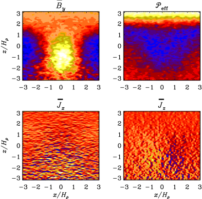
Figure 1: Representations of $\overline{B}_{y}$, ${\cal P}_{\rm eff}$, and the two components of $\overline{\mbox{\boldmath$J$}}{}$ in the $xz$ plane from a DNS with $\mbox{\rm Re}_{\rm M}=18$.

In all cases, we consider a weak imposed magnetic field in the $y$ direction. In Fig. 1 we show $y$-averaged visualizations of the normal component of the magnetic field, $\overline{B}_{y}$, together with the two components of the mean current density, $\overline{J}_{x}=-\partial\overline{B}_{y}/\partial z$, and $\overline{J}_{z}=\partial\overline{B}_{y}/\partial x$, and the normalized effective magnetic pressure, ${\cal P}_{\rm eff}=\Delta\overline{\Pi}_{xx}^{\rm f}/B_{\rm eq}^{2}$.

As a result of NEMPI, the field in the $xz$ plane gets concentrated in one position and diluted in another; see the first panel of Fig. 1. This leads to an equilibrium in which the resulting reduction of the turbulent pressure is offset by a corresponding increase in the gas pressure and therefore a corresponding increase in the density. The nonuniformity of the magnetic field implies a non-vanishing current density which is best seen in $\overline{J}_{z}$ (lower right panel of Fig. 1), but this is mainly because of enhanced fluctuations resulting from variations in the $z$ direction.

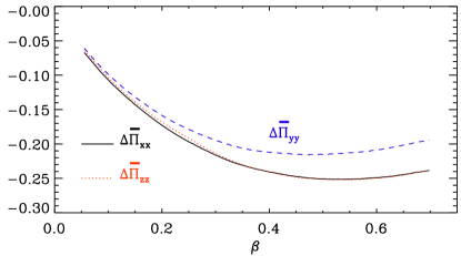
Figure 2: The 3 diagonal components of the tensor $\Delta\overline{\Pi}_{xx}^{\rm f}$ (solid, black), $\Delta\overline{\Pi}_{yy}^{\rm f}$ (dashed, blue), and $\Delta\overline{\Pi}_{zz}^{\rm f}$ (dotted, red), normalized by $B_{\rm eq}^{2}$ with a zero current density.

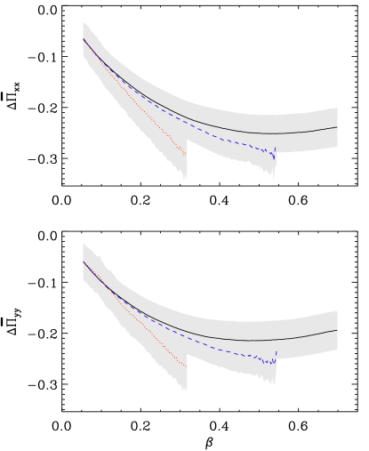
Figure 3: Normalized diagonal components $\Delta\overline{\Pi}_{xx}^{\rm f}$ and $\Delta\overline{\Pi}_{yy}^{\rm f}$ as a function of $\beta$, for vanishing mean current density (black, solid line), for points with low (dashed, blue, $0.25>\overline{J}^{2}H_{\rho}^{2}/B_{0}^{2}>0.1$) and higher current densities (dotted, red, 0.25 ¡ $J^{2}/H_{\rho}^{2}B_{0}^{2}$).

In Fig. 2 we show three diagonal components of the tensor $\Delta\overline{\Pi}_{xx}^{\rm f}$, $\Delta\overline{\Pi}_{yy}^{\rm f}$ and $\Delta\overline{\Pi}_{zz}^{\rm f}$, normalized by $B_{\rm eq}^{2}$ in turbulence with a zero mean current density. Fig. 2 demonstrates that the tensor $\Delta\overline{\Pi}_{yy}^{\rm f}$ in the direction of the mean magnetic field is different from the tensors $\Delta\overline{\Pi}_{xx}^{\rm f}$ and $\Delta\overline{\Pi}_{zz}^{\rm f}$ in the directions perpendicular to the mean magnetic field.

In the following we want to study the possible effects of current density on the resulting mean-field (or effective) magnetic pressure. We find that $\Delta\overline{\Pi}_{xz}^{\rm f}$ vanishes, which implies that $\tilde{q}_{\rm J}=0$; see Eq. (14). On the other hand, since $\Delta\overline{\Pi}_{xx}^{\rm f}\approx\Delta\overline{\Pi}_{zz}^{\rm f}$, the coefficient $q_{\rm g}$ vanishes or is small. In Fig. 3 we show two diagonal components $\Delta\overline{\Pi}_{xx}^{\rm f}$ and $\Delta\overline{\Pi}_{yy}^{\rm f}$, normalized by $B_{\rm eq}^{2}$ for different mean current densities. Inspection of Fig. 3 shows that the mean current density increases the negative minimum of the effective magnetic pressure characterized by $\Delta\overline{\Pi}_{xx}^{\rm f}$. This implies that an enhanced current density increases the effect of negative effective magnetic pressure, i.e., they intensify the formation of magnetic structures. Therefore, Eq. (11) allows us to determine $q_{\rm p}=-2\Delta\overline{\Pi}_{xx}^{\rm f}/\overline{B}^{2}$ and the mean effective magnetic pressure $p_{\rm eff}={\textstyle{1\over 2}}\left[1-q_{\rm p}(\beta)\right]\,\overline{B}^{2}=\Delta\overline{\Pi}_{xx}^{\rm f}+{\textstyle{1\over 2}}\overline{B}^{2}$. In agreement with earlier studies [5], we find a clear negative minimum in ${\cal P}_{\rm eff}(\beta)$ at $\beta\approx 0.25$. However, as the current density increases, the minimum of ${\cal P}_{\rm eff}(\beta)$ deepens, suggesting that NEMPI might turn out to be stronger than originally anticipated based on the dependence ${\cal P}_{\rm eff}(\beta)$ that does not distinguish between strong and weak current densities. A reasonable fit to such a behavior would be of the form

$$\overline{\Pi}_{xx}=-{\textstyle{1\over 2}}(1+\overline{J}^{2}/k_{J}^{2}B_{\rm eq}^{2})q_{\rm p}(\beta)\,\overline{B}^{2},$$ (18)

where $k_{J}$ is a free parameter. In Fig. 4 we show that we can get a good fit to the data for $k_{J}H_{\rho}=4$. Note further that equation (12) has two unknowns $\tilde{q}_{\rm I}$ and $q_{\rm s}$ which cannot be determined for such a simple configuration of the mean magnetic field, $\overline{\mbox{\boldmath$B$}}{}=(0,\overline{B}_{y}(x,z),0)$.

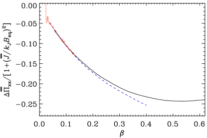
Figure 4: Like Fig. 3, but compensated by $1/(1+\overline{J}^{2}/k_{J}^{2}B_{\rm eq}^{2})$ for $k_{J}H_{\rho}=4$.

3.3 Gravity effects in DNS

We mention in passing the effect of changing gravity. It is clear that increasing gravity enhanced the anisotropy of the turbulence, which seems to have a reducing effect on the negative effective magnetic pressure; see Fig. 5. The reason for this is at the moment not well understood. We emphasize that this effect is connected with $q_{\rm p}$ and not with $q_{\rm g}$ that was introduced in equation (4).

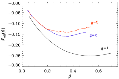
Figure 5: Dependence of ${\cal P}_{\rm eff}(\beta)$ on the value of $g$ (in units of $k_{1}c_{\rm s}^{2}$). Note that the depth of the minimum decreases with increasing gravity.

3.4 MFS

Next, let us investigate the spatial variations of ${\cal P}_{\rm eff}$ in a corresponding MFS. We use the parameters $\beta_{\star}$ and $\beta_{p}$ that are appropriate in the regime investigated in the DNS above, namely $\eta_{\rm t0}/u_{\rm rms}H_{\rho}=10^{-2}$, corresponding to $k_{\rm f}H_{\rho}\approx 30$, $B_{0}/B_{\rm eq0}=0.4$, $\beta_{\star}=0.32$ and $\beta_{p}=0.05$. The result is shown in Fig. 6, where we plot in the upper panel the $xz$ dependence of ${\cal P}_{\rm eff}$. Since the domain is periodic in the $x$ direction, we were able to shift the position of the minimum such that it lies approximately at $x=0$. The white vertical line near $x=0$ and the horizontal white line near $z/H_{\rho}=-4.3$ indicate positions along which we plot in the next two panels ${\cal P}_{\rm eff}$ at three different times.

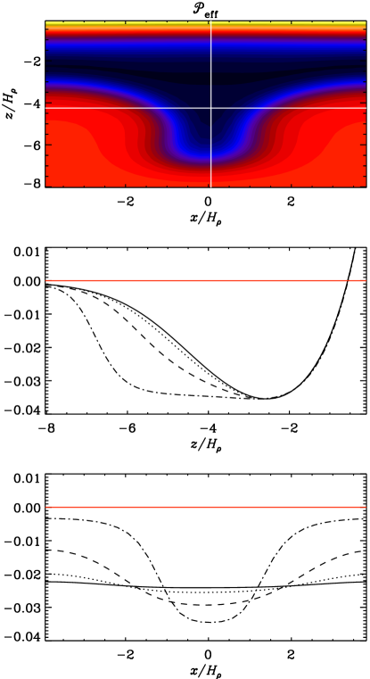
Figure 6: Representation of ${\cal P}_{\rm eff}$ in the $xz$ plane using a MFS with $\eta_{\rm t0}/u_{\rm rms}H_{\rho}=10^{-2}$, corresponding to $k_{\rm f}H_{\rho}\approx 30$, $B_{0}/B_{\rm eq0}=0.4$, $\beta_{\star}=0.32$ and $\beta_{p}=0.05$.

Initially, the minimum of ${\cal P}_{\rm eff}(\beta)$ occurs at the height $z/H_{\rho}\approx-2.5$, but at later times the minimum broadens and we have ${\cal P}_{\rm eff}\approx-0.035$ in the range $-5.5<z/H_{\rho}<2.5$. In the last panel of Fig. 6 we show that the horizontal extent of the structure becomes narrower and more concentrated as time goes on.

4 Conclusions

The present results have shown that NEMPI tends to develop sharp structures in the course of its nonlinear evolution. This becomes particularly clear from the MFS presented in §3.4. The results of §3.2 suggest that this might have consequences of an intensification of NEMPI with increasing $|\overline{\mbox{\boldmath$J$}}{}|$, as was demonstrated using DNS. At present it is not clear what is the appropriate parameterization of this effect. One possibility is that the $\overline{\mbox{\boldmath$J$}}{}$ dependence enters in the same way as the $\overline{\mbox{\boldmath$B$}}{}$ dependence, i.e., $\overline{\Pi}_{xx}=-{\textstyle{1\over 2}}(1+\overline{J}^{2}/k_{J}^{2}B_{\rm eq}^{2})q_{\rm p}(\beta)\,\overline{B}^{2}$, where we treat $k_{J}$ as a free parameter, although this might be a naive expectation given the small number of data points and experiments performed.

The present results are just a first attempt in going beyond the simple representation of the turbulent stress in terms if the mean field along. Other important terms include combinations with gravity as well as anisotropies of the form $\overline{J}_{i}\overline{J}_{j}$. Furthermore, if there is helicity, one could construct contributions to the stress tensor using products of the pseudo-tensors $\overline{J}_{i}\overline{B}_{j}$ and $\overline{J}_{j}\overline{B}_{i}$ with the kinetic or magnetic helicity. Such a construction obeys the fact that the Reynolds and Maxwell tensors are proper tensors. Such pseudo-tensors might play a role in the solar dynamo where the $\alpha$ effect is believed to play an important role. However, nothing is known about the importance or the sign of such effects. It would thus be desirable to have an accurate method that allows one to determine the relevant turbulent transport coefficients.

References

- Brandenburg [2005] Brandenburg A 2005, Astrophys. J. 625 539
- Brandenburg and Subramanian [2005] Brandenburg A and Subramanian K 2005, Phys. Rep., 417 1
- Brandenburg et al. [2010] Brandenburg A, Kleeorin N and Rogachevskii I 2010, Astron. Nachr. 331 5
- Brandenburg et al. [2011] Brandenburg A, Kemel K, Kleeorin N, Mitra D and Rogachevskii I 2011, Astrophys. J. 740 L50
- Brandenburg et al. [2012] Brandenburg A, Kemel K, Kleeorin N and Rogachevskii I 2012, Astrophys. J. 749 179
- Cally et al. [2003] Cally P S, Dikpati M and Gilman P A 2003, Astrophys. J. 582 1190
- Gilman and Dikpati [2000] Gilman P A and Dikpati M 2000, Astrophys. J. 528 552
- Käpylä et al. [2012a] Käpylä P J, Mantere M J and Brandenburg A 2012a, Astrophys. J. Lett., in press, arXiv:1205.4719
- Käpylä et al. [2012b] Käpylä P J, Brandenburg A, Kleeorin N, Mantere M J and Rogachevskii I 2012b, Mon. Not. R. Astron. Soc.422 2465
- Kemel et al. [2012a] Kemel, K., Brandenburg, A., Kleeorin, N. and Rogachevskii, I. 2012, Astron. Nachr. 333 95
- Kemel et al. [2012b] Kemel K, Brandenburg A, Kleeorin N, Mitra D and Rogachevskii I 2012b, Solar Phys. DOI:10.1007/s11207-012-0031-8, arXiv:1203.1232
- Kemel et al. [2012c] Kemel K, Brandenburg A, Kleeorin N, Mitra D and Rogachevskii I 2012c, Solar Phys. DOI:10.1007/s11207-012-9949-0, arXiv:1112.0279
- Kitchatinov & Mazur [2000] Kitchatinov LL, Mazur MV 2000, Solar Phys. 191 325
- Kleeorin et al. [1989] Kleeorin N, Rogachevskii I and Ruzmaikin A 1989, Sov. Astron. Lett. 15 274
- Kleeorin et al. [1990] Kleeorin N, Rogachevskii I and Ruzmaikin A 1990, Sov. Phys. JETP 70 878
- Kleeorin et al. [1993] Kleeorin N, Mond M and Rogachevskii I 1993, Phys. Fluids B, 5, 4128
- Kleeorin et al. [1996] Kleeorin N, Mond M and Rogachevskii I 1996, Astron. Astrophys. 307 293
- Kleeorin and Rogachevskii [1994] Kleeorin N and Rogachevskii I 1994, Phys. Rev. E 50 2716
- Krause and Rädler [1980] Krause F and Rädler K-H 1980, Mean-field magnetohydrodynamics and dynamo theory (Pergamon Press, Oxford)
- Losada [2012] Losada I R, Brandenburg A, Kleeorin N, Mitra D and Rogachevskii I 2012, Astron. Astrophys. (submitted), arXiv:1207.5392
- Moffatt [1978] Moffatt H K 1978, Magnetic field generation in electrically conducting fluids (Cambridge University Press, Cambridge)
- Parker [1979] Parker E N 1979, Cosmical magnetic fields (Oxford University Press, New York)
- Parfrey and Menou [2007] Parfrey K P and Menou K 2007, Astrophys. J. 667 L207
- Rogachevskii & Kleeorin [2007] Rogachevskii I and Kleeorin N 2007, Phys. Rev. E 76 056307
- Stein and Nordlund [2012] Stein R F and Nordlund Å 2012, Astrophys. J. 753 L13
- Zeldovich et al. [1983] Zeldovich Ya B, Ruzmaikin A A and Sokoloff D D 1983, Magnetic fields in astrophysics (Gordon & Breach, New York)