Phase diagram and critical points of a double quantum dot

Abstract

We apply a combination of numerical renormalization group (NRG) and renormalized perturbation theory (RPT) to a model of two quantum dots (impurities) described by two Anderson impurity models hybridized to their respective baths. The dots are coupled via a direct interaction $U_{12}$ and an exchange interaction $J$. The model has two types of quantum critical points, one at $J=J_{c}$ to a local singlet state and one at $U_{12}=U_{12}^{c}$ to a locally charge ordered state. The renormalized parameters which determine the low energy behavior are calculated from the NRG. The results confirm the values predicted from the RPT on the approach to the critical points, which can be expressed in terms of a single energy scale $T^{*}$ in all cases. This includes cases without particle-hole symmetry, and cases with asymmetry between the dots, where there is also a transition at $J=J_{c}$. The results give a comprehensive quantitative picture of the behavior of the model in the low energy Fermi liquid regimes, and some of the conclusions regarding the emergence of a single energy scale may apply to a more general class of quantum critical points, such as those observed in some heavy fermion systems.

I Introduction

Experimental evidence in heavy fermion materials suggests that there is a close connection between the regions of anomalous spin fluctuations associated with a quantum critical point and the occurrence of superconductivity. There is a similar association in the cuprates Tai10 and iron pnictide Ste11 superconductors. This has motivated many experimental studies of quantum behavior in fermionic systems, which can be induced by lowering the transition in a magnetically ordered state to zero by application of pressure, a magnetic field or by alloyingSS10 ; LRVW07 ; CPSR01 . Many conjectures have been put forward to understand this behavior, but as yet there is no fully quantitative or comprehensive explanation (for a recent review on this topic see referenceSS10 ). This situation has led to a resurgence of interest in local or impurity models which have quantum critical points. There are two reasons for this. Firstly, impurity problems are simpler and well established techniques have been developed for tackling them. Secondly, such systems can be simulated using nanoscale devices, such as quantum dots, where the parameters can be varied in a controlled way via gate voltages and the behavior examined over different regimes. An example is the two channel Kondo model, which has a quantum critical point and non-Fermi liquid behavior. An arrangement of quantum dots and gate voltages has been used successfully to test experimentally theoretical predictions for this model in the non-Fermi liquid regimePRSOD07 .

The two impurity Kondo model is another example of a model with local quantum critical behavior. Numerical renormalization group studies for this model have shown that there is a discontinuous transition on increasing the (antiferromagnetic) exchange interaction between the two impurities from a state in which the impurity spins are predominantly screened by the conduction electrons (Kondo screening) to one screened within a local singlet stateJV87 . There has been recent experimental workBZD11 to examine the critical behavior of this model using two magnetic impurities, one on a STM tip and the other on a metal surface, such that the interaction between the two impurities can be modified by controlling the distance of the STM tip from the surface. Yet another type of critical point which has been studied theoreticallyGLK06 , one that could occur in two capacitatively coupled quantum dots, has a discontinuous transition to a locally charge ordered state.

In a recent paper we studied a two-impurity Anderson model which has direct and exchange interactions between the two impurities and displays both types of transitionNCH12 . We showed, by using a combination of renormalized perturbation theory (RPT) and numerical renormalization group calculations (NRG), that we could derive many exact results for the low temperature behavior in the Fermi liquid regime right up to the quantum critical points. We were able to show the emergence of a single energy scale on the approach to each type of quantum critical point with renormalized Fermi liquid parameters corresponding to a strong correlation regime. The results were restricted to a model with symmetry between the two impurities and particle-hole symmetry. In this paper we enlarge upon those results, examine the phase diagram more fully, and also relax the restrictions to include channel asymmetry and lack of particle-hole symmetry.

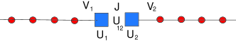
Figure 1: (Color online) A schematic illustration of NRG chains for the double dot system. The quantum dots (filled squares) interact via an exchange $J$ and a direct term $U_{12}$, and are hybridized with the first site of their respective conduction electron chains (filled circles).

The model for the system we study corresponds to two quantum dots connected via leads with their respective conduction baths. The Hamiltonian ${\cal H}$ for the system takes the form ${\cal H}={\cal H}_{1}+{\cal H}_{2}+{\cal H}_{12}$, where the individual dots are described by a single impurity Anderson model, so ${\cal H}_{\alpha}$ for dot $\alpha=1,2$ is given by

$${\cal H}_{\alpha}=\sum_{\sigma}\epsilon_{d,\alpha}d^{\dagger}_{\alpha,\sigma}d_{\alpha,\sigma}+\sum_{k,\sigma}\epsilon_{k,\alpha}c^{\dagger}_{k,\alpha,\sigma}c_{k,\alpha,\sigma}$$ (1)

$$+\sum_{k,\sigma}(V_{k,\alpha}d^{\dagger}_{\alpha,\sigma}c_{k,\alpha,\sigma}+V_{k,\alpha}^{*}c^{\dagger}_{k,\alpha,\sigma}d_{\alpha,\sigma})+U_{\alpha}n_{d,\alpha,\uparrow}n_{d,\alpha,\downarrow}$$

where $d^{\dagger}_{\alpha,\sigma}$, $d_{\alpha,\sigma}$, are creation and annihilation operators for an electron at the impurity site in channel $\alpha$, where $\alpha=1,2$, and spin component $\sigma=\uparrow,\downarrow$. The creation and annihilation operators, $c^{\dagger}_{k,\alpha,\sigma}$, $c_{k,\alpha,\sigma}$, are for conduction electrons with energy $\epsilon_{k,\alpha}$ in channel $\alpha$. The hybridization function for each dot is given by $\Delta_{\alpha,\sigma}(\omega)=\pi\sum_{k}|V_{k,\alpha}|^{2}\delta(\omega-\epsilon_{k})$. We will make the usual approximation and take $\Delta_{\alpha,\sigma}(\omega)$ to be a constant $\Delta_{\alpha}$, independent of $\omega$ and $\sigma$, corresponding to the wide band limit with a constant density of states.

The interaction between the two quantum dots is taken in the form of a direct term $U_{12}$, and an exchange term $J$, so that the interaction Hamiltonian ${\cal H}_{12}$ has the form,

$${\cal H}_{12}=U_{12}\sum_{\sigma}n_{d,1,\sigma}\sum_{\sigma^{\prime}}n_{d,2,\sigma^{\prime}}+2J{\bf S}_{d,1}\cdot{\bf S}_{d,2},$$ (2)

where $J>0$ for an antiferromagnetic coupling and $J<0$ in the ferromagnetic case.

Though the model here is taken to describe a double quantum dot, it can serve equally well to describe a number of other physical situations. It can describe a single magnetic impurity with two fold ’orbital’ degeneracy, where the exchange coupling $J$ then corresponds to a Hund’s rule term where a ferromagnetic exchange term would be appropriate Yos76 ; NCH10s ; NCH10a . In the strong coupling regime $U/\pi\Delta\gg 1$, the model corresponds to two Kondo models and with $U_{12}=0$ it has been much studied as a model of a system with two coupled magnetic impurities JV87 ; JV89 ; SVK93 ; Gan95 . The model with $J=0$ has also been used to study two capacitatively coupled quantum dots GLK06 .

For the numerical renormalization group calculations (NRG) the conduction electron states are transformed to a basis corresponding to a tight-binding chain such that the model takes the form illustrated in Fig 1. The densities of states for the conduction electron baths (half-bandwidth $D$) are discretized with a parameter $\Lambda(>1)$ as in the original calculation of Wilson Wil75 so that the couplings along the chain fall off as $\Lambda^{-N/2}$, for large $N$, where $N$ is the $N$th site along the chain from the dot.

II Phase Diagram

As the model used here is rather more general than those studied so far, we show some results for the phase diagram which now includes two QCPs. Before considering the general case we look at the case with $U_{12}=0$. In the Kondo regime this is a much studied model of a system with two coupled magnetic impurities JV87 ; JV89 ; SVK93 ; Gan95 which has a QCP at $J=J_{c}$ where there is a sudden change in phase shift of the conduction electrons from $\pi/2$ to zero. When $J=0$ the two dots are isolated and their ground states are (Kondo) singlets giving a phase shift of $\pi/2$ in each channel. In the opposite limit $J\to\infty$ the impurity spins form a decoupled local singlet such that the phase shift of the conduction electrons in each channel is zero. In some related models the change between these two limits was found to occur continuously with increase of $J$. Affleck, Ludwig and Jones AL92 ; ALJ95 , however, cleared up the confusion resulting from apparently conflicting results from the different models, in giving the conditions for the change to occur discontinuously, resulting in a QCP. In a more recent study of a quantum dot version of the model, it has been shown that the transition occurs even when there is asymmetry between the two channels and away from particle-hole symmetryZCSV06 . For the calculations of the phase diagram we assume both channel symmetry $U_{1},V_{1}=U_{2},V_{2}$ and particle-hole symmetry $\epsilon_{d,\alpha}=-U_{\alpha}/2$, though we relax some of these conditions later. It will be useful to introduce a renormalised quantity $\tilde{\Delta}(0)$, which will be defined more fully later, such that $\tilde{\Delta}(U,0)\to\Delta$ for $U\to 0$ and in the Kondo regime $U/\pi\Delta\gg 1$, $\pi\tilde{\Delta}(U,0)\to 4T_{\rm K}$, where $T_{\rm K}$ the Kondo temperature of the isolated dot, defined by the relation $T_{\rm K}=(g\mu_{\rm B})^{2}/4\chi_{\rm imp}$, where $\chi_{\rm imp}$ is the $T=0$ spin susceptibility for an isolated dot.

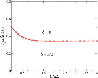
Figure 2: (Color online) A plot of $J_{c}/\pi\tilde{\Delta}(U,0)$ as a function of $U/\pi\Delta$ for $\pi\Delta=0.01$.

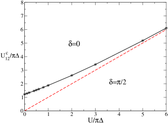
Figure 3: (Color online) A plot of $U^{c}_{12}/\pi\Delta$, as a function of $U/\pi\Delta$ for the model with $J=0$.

In Fig. 2 we give a plot of the critical value $J_{c}/\pi\tilde{\Delta}(U,0)$ as a function of $U/\pi\Delta$ for $\pi\Delta=0.01$ (note: we take this value for $\pi\Delta$ all subsequent calculations unless specified explicitly). The transition in the NRG calculations corresponds to a sudden change in the low energy fixed point from that of a free chain with $N$ sites, where $N$ is even (odd) to one with $N$ odd (even). It can be seen that there is a transition for all values of $U$ including $U=0$. For $U/\pi\Delta>3$ the curve is flat indicating that in this regime $J_{c}$ is proportional to $T_{\rm K}$, corresponding to $J_{c}=1.378T_{\rm K}$. These results are in line with calculations based on the Kondo model where values of $J_{c}/T_{\rm K}\approx 1.4$ were estimated when expressed using our definition of $T_{\rm K}$ JV87 ; JV89 ; SVK93 (in previous studies $T_{\rm K}$ was defined by $\chi_{s}=2\mu_{\rm B}^{2}/\pi T_{\rm K}$ giving in our case $J_{c}/T_{\rm K}=2.165$).

The second type of transition to a local charge ordered state occurs in the model $J=0$ when $U_{12}$ reaches a critical value $U^{c}_{12}$. For $U_{12}=0$ the charges on the two impurities are identical, but on increasing $U_{12}$ such that $U_{12}\gg U$ it becomes energetically unfavourable and there is a local broken symmetry resulting in a charge imbalance between the impurities. If there are matrix elements connecting the two possible broken symmetry states to restore the symmetry then they must be exceedingly small because the NRG results indicate a precise transition at a critical value $U_{12}=U^{c}_{12}$. We plot the value of $U^{c}_{12}/\pi\Delta$ as a function of $U/\pi\Delta$ in Fig. 3. This transition exists for all values of $U$ and for $U/\pi\Delta\gg 3$ the critical values approach the value of $U$, i.e. $U^{c}_{12}\to U$. These results are in agreement with those given earlier by Galpin et al. GLK06 .

The phase diagram for the model with finite $J$ and $U_{12}$, where both types of transitions occur, is shown in Fig.4 for the value $U/\pi\Delta=5$. The two types of transition are separated by the line $U_{12}=U+3J/2$ along which the phase shift remains at the value $\delta=\pi/2$. The two types of transition asymptotically approach this line on opposite sides.

To investigate the low energy behavior of the model in detail, we first derive a number of exact results in terms of renormalized parameters using a renormalized perturbation theory (RPT) for the low energy properties in the Fermi liquid regime. An analysis of the low energy NRG fixed point is then used to calculate the renormalized parameters in terms of the ‘bare’ parameters that define the model. Once the renormalized parameters have been calculated, they can be substituted into the equations for the exact evaluation of the low energy thermodynamics. The relevant equations based on the renormalized pertubation theory (RPT) will be derived in the next section.

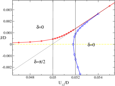
Figure 4: (Color online) A plot of the critical lines (local singlet- stars, local charge order - circles) separating the regions with phase shift $\delta=\pi/2$ and $\delta=0$ as a function of $J/D$ and $U_{12}/D$ for $U/\pi\Delta=5$. The dotted line corresponds to $U_{12}=U+3J/2$. The two vertical lines relate to results shown later in Fig. 26 and Fig. 27.

III RPT Analysis

We start with the Fourier transform of the single particle Green’s function for the impurity $d$-state,

$$G_{d,\alpha,\sigma}(\omega_{n^{\prime}})=-\int_{0}^{\beta}\langle T_{\tau}d_{\alpha,\sigma}(\tau)d^{\dagger}_{\alpha,\sigma}(0)\rangle e^{i\omega_{n^{\prime}}\tau}\,d\tau,$$ (3)

where $\omega_{n^{\prime}}=(2n^{\prime}+1)/\beta$ and $\beta=1/T$ and the brackets $\langle...\rangle$ denote a thermal average. This Green’s function can be expressed in the form,

$$G_{d,\alpha,\sigma}(\omega_{n})={1\over i\omega_{n}-\epsilon_{d,\alpha}+i\Delta_{\alpha,\sigma}{\rm sgn}(\omega_{n})-\Sigma_{\alpha,\sigma}(\omega_{n})},$$ (4)

where $\Sigma_{\alpha,\sigma}(\omega_{n})$ is the self-energy.

For the zero temperature Green’s function, which will be our main concern, $\omega_{n}$ can be replaced by a continuous variable $\omega$, and summations over $\omega_{n}$ replaced by integrations over $\omega$. For the renormalized perturbation theory Hew93 , the Green’s function in Eq.(4) can be re-expressed as $G_{d,\alpha,\sigma}(\omega_{n})=z_{\alpha}\tilde{G}_{d,\alpha,\sigma}(\omega_{n})$, where $\tilde{G}_{d,\alpha,\sigma}(\omega_{n})$ is the quasiparticle Green’s function given by

$$\tilde{G}_{d,\alpha,\sigma}(\omega_{n})={1\over i\omega_{n}-\tilde{\epsilon}_{d,\alpha}+i\tilde{\Delta}_{\alpha}{\rm sgn}(\omega_{n})-\tilde{\Sigma}_{\alpha,\sigma}(\omega_{n})}$$ (5)

and the renormalized parameters, $\tilde{\epsilon}_{d,\alpha}$ and $\tilde{\Delta}_{\alpha}$ are given by

$$\tilde{\epsilon}_{d,\alpha}=z_{\alpha}(\epsilon_{d,\alpha}+\Sigma_{\alpha,\sigma}(0)),\quad\tilde{\Delta}_{\alpha}=z_{\alpha}\Delta_{\alpha},$$ (6)

where $z_{\alpha}=1/(1-\partial\Sigma_{\alpha,\sigma}(\omega)/\partial(i\omega))$ evaluated at $\omega=0$. The quasiparticle self-energy $\tilde{\Sigma}_{\alpha,\sigma}(\omega)$ is given by

$$\tilde{\Sigma}_{\alpha,\sigma}(\omega)=$$

$$z_{\alpha}\left(\Sigma_{\alpha,\sigma}(\omega)-\Sigma_{\alpha,\sigma}(0)-i\omega{\partial\Sigma_{\alpha,\sigma}(\omega)\over\partial i\omega}\Big{|}_{\omega=0}\right),$$

where we have assumed the Luttinger theorem Lut60 , ${\rm Im}\Sigma(0)=0$, so that ${\rm Im}\tilde{\Sigma}_{\alpha,\sigma}(\omega)\sim\omega^{2}$ as $\omega\to 0$. When expressed in this form, the $\omega=0$ part of the self-energy and its derivative have been absorbed into renormalizing the parameters $\epsilon_{d,\alpha}$ and $\Delta_{\alpha}$, so in setting up the perturbation expansion any further renormalization of these terms must be excluded, or it will result in over-counting. In working with the fully renormalized quasiparticles it is appropriate to use the renormalized or effective interactions between the quasiparticles. In the single channel case, we identify the renormalized interaction $\tilde{U}_{\alpha}$ as the local four vertex $\Gamma^{\alpha}_{\uparrow,\downarrow,\downarrow,\uparrow}(\omega_{1},\omega_{2},\omega_{3},\omega_{4})$ in the zero frequency limit Hew93 ,

$$\tilde{U}_{\alpha}=z_{\alpha}^{2}\Gamma^{\alpha}_{\uparrow,\downarrow,\downarrow,\uparrow}(0,0,0,0).$$ (7)

In this case we need to include the local inter-channel four vertex, $\Gamma^{\alpha\alpha^{\prime}}(\omega_{1},\omega_{2})$ corresponds to the Fourier coefficient of the connected skeleton diagram for the two particle Green’s function,

$$\langle T_{\tau}{\bf S}_{d,1}(\tau_{1})\cdot{\bf S}_{d,2}(\tau_{2})\rangle,$$ (8)

with the external legs removed. We define

$$2\tilde{J}=z_{1}z_{2}\Gamma_{{\bf\sigma_{1}},{\bf\sigma}_{2}}(0,0,0,0).$$ (9)

and we can define a renormalized direct interaction $\tilde{U}_{12}$ in a similar way.

We can combine these terms to define a quasiparticle Hamiltonian $\tilde{\cal H}=\sum_{\alpha}\tilde{\cal H}_{\alpha}+\tilde{\cal H}_{12}$, where

$$\tilde{\cal H}_{\alpha}=\sum_{\sigma}\tilde{\epsilon}_{d,\alpha}\tilde{d}^{\dagger}_{\alpha,\sigma}\tilde{d}_{\alpha,\sigma}+\sum_{k\sigma}\epsilon_{k,\alpha}c^{\dagger}_{k,\alpha,\sigma}c_{k,\alpha,\sigma}$$

$$+\sum_{k,\sigma}(\tilde{V}_{k}\tilde{d}^{\dagger}_{\alpha,\sigma}c_{k,\alpha,\sigma}+\tilde{V}_{k}^{*}c^{\dagger}_{k,\alpha,\sigma}\tilde{d}_{\alpha,\sigma})+\tilde{U}_{\alpha}:\tilde{n}_{d,\alpha,\uparrow}\tilde{n}_{d,\alpha,\downarrow}:$$

and

$$\tilde{\cal H}_{12}=\tilde{U}_{12}:\sum_{\sigma}\tilde{n}_{d,1,\sigma}\sum_{\sigma^{\prime}}\tilde{n}_{d,2,\sigma^{\prime}}:+2\tilde{J}:\tilde{\bf S}_{d,1}\cdot\tilde{\bf S}_{d,2}:,$$ (10)

The brackets :${\hat{O}}$: indicate that the operator ${\hat{O}}$ within the brackets must be normal ordered with respect to the ground state of the interacting system, which plays the role of the vacuum. This is because the interaction terms only come into play when more than one quasiparticle is created from the vacuum.

The renormalized Hamiltonian is not equivalent to the original model, and the relation between the original and renormalized model is best expressed in the Lagrangian formulation, where frequency enters explicitly Hew01 . If the Lagrangian density ${\cal L}(\epsilon_{d},\Delta_{\alpha},U,J)$ describes the original model, then by suitably re-arranging the terms we can write

$${\cal L}(\epsilon_{d},\Delta,U,J,U_{12})={\cal L}(\tilde{\epsilon}_{d},\tilde{\Delta}_{\alpha},\tilde{U}_{\alpha},\tilde{J},\tilde{U}_{12})+{\cal L}_{c}(\{\lambda_{i}\}),$$ (11)

where the remainder part ${\cal L}_{c}(\{\lambda_{i}\})$ is known as the counter term. The set of coefficients $\{\lambda_{i}\}$, where $i=1,2,3,4,5$, can be expressed explicitly in terms of the self-energy terms and vertices at zero frequency. These relations, however, are not useful in carrying out the expansion. We want to work entirely with the renormalized parameters and carry out the expansion in powers of $\tilde{U}_{\alpha}$, $\tilde{J}$ and $\tilde{U}_{12}$. We assume that the $\lambda_{i}$ can be expressed in powers of quasiparticle interaction terms, $\tilde{U}_{\alpha}$, $\tilde{J}$ and $\tilde{U}_{12}$, and can be determined order by order from the conditions that there should be no further renormalization of quantities which have already been taken to be fully renormalized. These conditions are

$$\tilde{\Sigma}_{\alpha,\sigma}(0)=0,\quad{\partial\tilde{\Sigma}_{\alpha,\sigma}(\omega)\over\partial i\omega}\Big{|}_{0}=0,$$ (12)

and that the renormalized local and intersite 4-vertices at zero frequency are unchanged.

The propagator in the RPT is the free quasiparticle Green’s function,

$$\tilde{G}^{(0)}_{d,\alpha,\sigma}(\omega_{n})={1\over i\omega_{n}-\tilde{\epsilon}_{d,\alpha}+i\tilde{\Delta}_{\alpha}{\rm sgn}(\omega_{n})}.$$ (13)

From Fermi liquid theory, the quasiparticle interaction terms do not contribute to the linear specific heat coefficient $\gamma$ of the electrons. The specific heat coefficient $\gamma$ is given by

$$\gamma=2\pi^{2}\sum_{\alpha}\tilde{\rho}_{\alpha}(0)/3,$$ (14)

where $\tilde{\rho}_{\alpha}(\omega)$ is the free quasiparticle density of states per single spin and channel,

$$\tilde{\rho}_{\alpha}(\omega)={\tilde{\Delta}_{\alpha}/\pi\over(\omega-\tilde{\epsilon}_{d,\alpha})^{2}+\tilde{\Delta}_{\alpha}^{2}}.$$ (15)

The results for the spin susceptibility is given by

$$\chi_{s}=2\mu_{\rm B}^{2}\sum_{\alpha}\tilde{\eta}_{s,\alpha}\tilde{\rho}_{\alpha}(0),\quad\chi_{c}=2\sum_{\alpha}\tilde{\eta}_{c,\alpha}\tilde{\rho}_{\alpha}(0),$$ (16)

where

$$\tilde{\eta}_{s,\alpha}=1 + \tilde{U}_{\alpha}\tilde{\rho}_{\alpha}(0)-\tilde{J}\tilde{\rho}_{\beta}(0),$$

$$\tilde{\eta}_{c,\alpha}=1 - \tilde{U}_{\alpha}\tilde{\rho}_{\alpha}(0)-2\tilde{U}_{12}\tilde{\rho}_{\beta}(0),$$ (17)

where $\beta\neq\alpha$. The equations for the spin and charge susceptibilities, $\chi_{s}$ and $\chi_{c}$, can be proved using the Ward identities which follow from conservation of total spin and charge. They also correspond to a simple mean field approximation to first order in the effective interactions, $\tilde{U}_{\alpha}$, $\tilde{J}$ and $\tilde{U}_{12}$, in the quasiparticle Hamiltonian Eqn. (10). The corresponding equations for the staggered susceptibilities also follow from these mean field equations and in the Appendix we give an alternative way they can be derived from the leading correction terms to the NRG fixed point,

$$\chi^{st}_{s}=2\mu_{\rm B}^{2}\sum_{\alpha}\tilde{\eta}^{st}_{s,\alpha}\tilde{\rho}_{\alpha}(0),\quad\chi^{st}_{c}=2\sum_{\alpha}\tilde{\eta}^{st}_{c,\alpha}\tilde{\rho}_{\alpha}(0),$$ (18)

where

$$\tilde{\eta}^{st}_{s,\alpha}=1 + \tilde{U}_{\alpha}\tilde{\rho}_{\alpha}(0)+\tilde{J}\tilde{\rho}_{\beta}(0),$$

$$\tilde{\eta}^{st}_{c,\alpha}=1 - \tilde{U}_{\alpha}\tilde{\rho}_{\alpha}(0)+2\tilde{U}_{12}\tilde{\rho}_{\beta}(0).$$ (19)

From the equation of motion of the Green’s function $G^{\alpha}_{k\sigma,k^{\prime},\sigma}(\omega)$, which is the Fourier transform of the retarded conduction electron Green’s function $<<c_{\alpha,k,\sigma}(t):c_{\alpha,k^{\prime},\sigma}^{\dagger}(t^{\prime})>>$ in channel $\alpha$, we can derive the equation,

$$G^{\alpha}_{k\sigma,k^{\prime},\sigma}(\omega)={\delta_{k,k^{\prime}}\over(\omega-\epsilon_{k})}+{1\over(\omega-\epsilon_{k})}t^{k,k^{\prime}}_{\alpha,\sigma}(\omega){1\over(\omega-\epsilon_{k^{\prime})}},$$ (20)

where the t-matrix, $t^{k,k^{\prime}}_{\alpha,\sigma}(\omega)$ is given by $t^{k,k^{\prime}}_{\alpha,\sigma}(\omega)=V_{k,\alpha}G_{d,\alpha,\sigma}(\omega)V_{k^{\prime},\alpha}$. From the definition of the phase shift as the phase of the t-matrix for $\omega=0$,

$$\delta_{\alpha,\sigma}={\rm tan}^{-1}\left({{\rm Im}\,G_{d,\alpha,\sigma}(0)\over{\rm Re}\,G_{d,\alpha,\sigma}(0)}\right),$$ (21)

we find

$$\delta_{\alpha}-{\pi\over 2}=-{\rm tan}^{-1}\left({\epsilon_{d,\alpha}+\Sigma_{\alpha}(0)\over\Delta_{\alpha}}\right)=-{\rm tan}^{-1}\left({\tilde{\epsilon}_{d,\alpha}\over\tilde{\Delta}_{\alpha}}\right).$$ (22)

The total occupation of the impurity sites $\sum n_{d,\alpha}=\sum\delta_{\alpha}/\pi$ at $T=0$, which corresponds to the Friedel sum rule.

We consider first of all the model with $U_{12}=J=0$, which corresponds to two independent Anderson models. With particle-hole symmetry $\epsilon_{d,\alpha}=-U_{\alpha}/2$, $\tilde{\epsilon}_{d,\alpha}=0$, which corresponds to a phase shift $\delta_{\alpha}=\pi/2$ in a given spin channel, independent of the value of $U_{\alpha}$. This leaves just two renormalized parameters per dot, $\tilde{\Delta}_{\alpha}$ and $\tilde{U}_{\alpha}$, which are related in the strong coupling regime, as there is only one relevant low energy scale, the Kondo temperature $T_{\rm K,\alpha}$. The relation takes the form, $\tilde{U}_{\alpha}=\pi\tilde{\Delta}_{\alpha}=4T_{\rm K,\alpha}$, where $T_{\rm K,\alpha}$ is defined such that spin susceptibility of a single impurity is given by $\chi_{s,\alpha}=(g\mu_{\rm B})^{2}/4T_{\rm K,\alpha}$.

On the approach to a quantum critical point we expect both quasiparticle weight factors, $z_{1}\to 0$ and $z_{2}\to 0$, as a singularity develops in the self-energy of the dot Green’s functions, which implies a divergence in the specific heat coefficient $\gamma$. It also implies a divergence in the quasiparticle density of states at the Fermi level, $\tilde{\rho}_{\alpha}(0)\to\infty$. As $J\to J_{c}$ we expect a divergence in the staggered spin susceptibility $\chi_{s}^{st}$ as it is the fluctuations in this channel that become critical. We expect the other susceptibilities, $\chi_{s}$, $\chi_{c}$ and $\chi_{c}^{st}$, to remain finite, which leads us to require $\eta_{s,\alpha}\to 0$, $\eta_{c,\alpha}\to 0$ and $\eta_{c,\alpha}^{st}\to 0$ as $J\to J_{c}$. These conditions give sufficient equations for us to determine all the renormalized parameters $\tilde{\rho}_{\alpha}(0)$, $\tilde{U}_{\alpha}$, $\tilde{J}$ and $\tilde{U}_{12}$ in terms of a single energy scale. We find

$$\tilde{U}_{\alpha}\tilde{\rho}_{\alpha}(0)\to 1,\quad\tilde{J}\tilde{\rho}_{\alpha}(0)\to 2,\quad\tilde{U}_{12}\tilde{\rho}_{\alpha}(0)\to 0.$$ (23)

For the local charge transition it is only the the staggered charge susceptibility $\chi_{c}^{st}$ which should diverge as $U_{12}\to U^{c}_{12}$. For the other susceptibilities to remain finite, $\eta_{s,\alpha}\to 0$, $\eta_{c,\alpha}\to 0$ and $\eta_{c,\alpha}^{st}\to 0$ as $U_{12}\to U^{c}_{12}$. This implies

$$\tilde{U}_{\alpha}\tilde{\rho}_{\alpha}(0)\to-1,\quad\tilde{J}\tilde{\rho}_{\alpha}(0)\to 0,\quad\tilde{U}_{12}\tilde{\rho}_{\alpha}(0)\to 1.$$ (24)

We can define an energy scale $T^{*}$ as $J\to J_{c}$ on the approach to the QCPs via $1/\tilde{\rho}(0)=4T^{*}$ which for particle-hole symmetry becomes $\pi\tilde{\Delta}=4T^{*}$, such that the renormalized interaction parameters can be expressed in terms of this single energy scale $T^{*}$.

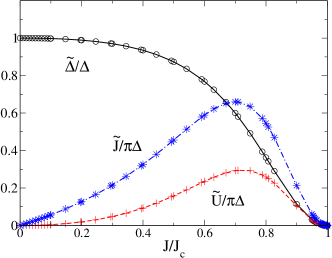
Figure 5: (Color online) A plot of $\tilde{\Delta}/\Delta$, $\tilde{U}/\pi\Delta$ and $\tilde{J}/\pi\Delta$ as a function of $J/J_{c}$, for $U=0$.

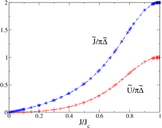
Figure 6: (Color online) A plot of the ratios, $\tilde{U}/\pi\tilde{\Delta}$ and, and $\tilde{J}/\pi\tilde{\Delta}$ as a function of $J/J_{c}$, for $U=0$.

Other exact results can be obtained from the RPT. An exact expression for the renormalized self-energy for the model with particle-hole symmetry $\tilde{\Sigma}(\omega)$ to order $\omega^{2}$ and $T^{2}$ follows from an RPT calculationNCH12 taken to second order in interaction parameters $\tilde{U}$, $\tilde{J}$ and $\tilde{U}_{12}$, and is given by

$$\tilde{\Sigma}(\omega,T)={-i\pi^{2}I\tilde{\Delta}\over 64}\left[\left({\omega\over T^{*}}\right)^{2}+\left({\pi T\over T^{*}}\right)^{2}\right],$$ (25)

where $I=(2\tilde{U}^{2}+3\tilde{J}^{2}+4\tilde{U}_{12}^{2})/(\pi\tilde{\Delta})^{2}$, so $I\to 14$ as $J\to J_{c}$ and $I\to 6$ as $U\to U_{12}^{c}$, and we have taken the channel symmetric case, $U_{1}=U_{2}$, $V_{1,k}=V_{2,k}$. This is a generalization of the calculations given earlier in a paper on an impurity model with a Hund’s rule term NCH10s ; Yos76 . On substituting (25) into the quasiparticle Green’s function, we deduce $\omega^{2}$ and $T^{2}$ contribution to the t-matrix, $t_{\alpha}(\omega,T)$,

$${i\pi D\over 16}\left[(I+4)\left({\omega\over T^{*}}\right)^{2}+I\left({\pi T\over T^{*}}\right)^{2}\right].$$ (26)

The ratio of the $\omega^{2}$ to the $\pi^{2}T^{2}$ term is $(I+4)/I$, which for $I=14$ gives $9/7$ in agreement with the calculation of Mitchell and SelaMS12 for the two impurity Kondo model.

To evaluate the RPT expressions for the low energy behavior of the model we need the values of the renormalized parameters in terms of the ‘bare’ parameters that define the model. We give a brief description how they may be deduced from the low energy fixed point in an NRG calculation. The results of these calculations enable us to test the predictions given in Eqns (23) and (24). An evaluation of the RPT expressions gives a comprehensive picture of the low energy behavior of the model in the Fermi liquid regimes.

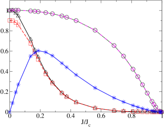
Figure 7: (Color online) A plot of $\tilde{\Delta}_{1}(U,J)/\tilde{\Delta}_{1}(U,0)$ (dotted line and triangles), $\tilde{\Delta}_{2}(U,J)/\tilde{\Delta}_{2}(U,0)$ (full line and circles), $\tilde{U}_{1}/\pi\tilde{\Delta}_{1}(U,0)$ (dashed line and squares), $\tilde{U}_{2}/\pi\tilde{\Delta}_{2}(U,0)$ (dot-dashed line and diamonds), and $\tilde{J}/\pi(\tilde{\Delta}_{1}(U,0)\tilde{\Delta}_{2}(U,0))^{1/2}$ (full line and stars) as a function of $J/J_{c}$, for $U/\pi\Delta_{2}=6$, $\Delta_{1}/\Delta_{2}=4$, $\Delta_{2}=0.01$.

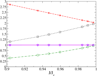
Figure 8: (Color online) A plot of $\tilde{J}/\pi\tilde{\Delta}_{1}$ (dots and squares), $\tilde{J}/\pi\tilde{\Delta}_{2}$ (dashes, stars), $\tilde{U}_{1}/\pi\tilde{\Delta}_{1}$(full line, up triangle), $\tilde{U}_{2}/\pi\tilde{\Delta}_{2}$ (full line, down triangle), and $\tilde{\Delta}_{2}/\tilde{\Delta}_{1}$ (dot-dash, circles) as a function of $J/J_{c}$ for $U/\pi\Delta_{2}=6$, $\Delta_{1}/\Delta_{2}=4$, $\pi\Delta_{2}=0.01$.

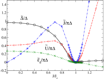
Figure 9: (Color online) A plot of $\tilde{\Delta}/\Delta$, $\tilde{\epsilon}_{d}/\pi\Delta$, $\tilde{U}/\pi\Delta$ and $\tilde{J}/\pi\Delta$ as a function of $J/J_{c}$, for $U/\pi\Delta=0.5$, $\epsilon_{d}/\pi\Delta=0.159$.

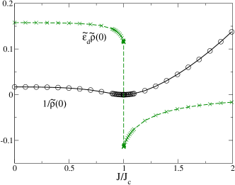
Figure 10: (Color online) A plot of $1/\tilde{\rho}(0)$ ($=4T^{*}$) and $\tilde{\epsilon}_{d}\tilde{\rho}(0)$ as a function of $J/J_{c}$, for $U/\pi\Delta=0.5$, $\epsilon_{d}/\pi\Delta=0.159$. The discontinuity in $\tilde{\epsilon}_{d}\tilde{\rho}(0)$ at the quantum critical point corresponds to a jump in phase shift of $\pi/2$ per spin state per dot channel.

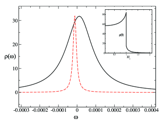
Figure 11: (Color online) A plot of low energy local dot spectral density $\rho(\omega)=z\tilde{\rho}(\omega)$ as a function of $\omega$ for the two cases $J/J_{c}=0.98$ (full curve) and $J/J_{c}=1.02$ (dashed curve) for the same parameter set as in Fig. 10. The inset shows $\rho(0)$ ($=z\tilde{\rho}(0)$) as a function of $J/J_{c}$ showing the discontinuous loss of spectral density at the Fermi level as the value of $J$ increases through the critical point $J=J_{c}$.

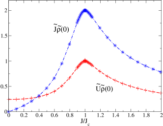
Figure 12: (Color online) A plot of $\tilde{U}\tilde{\rho}(0)$ and $\tilde{J}\tilde{\rho}(0)$ as a function of $J/J_{c}$, for $U/\pi\Delta=0.5$, $\epsilon_{d}/\pi\Delta=0.159$.

IV NRG Calculation of Renormalized Parameters

The numerical renormalization group results can be used to calculate the renormalized parameters, by identifying the quasiparticle Hamiltonian in Eqn. (10) as the NRG low energy fixed point with the leading order correction terms. In the NRG calculation the non-interacting Green’s function for the impurity site $\alpha$ takes the form,

$$G^{(0)}_{d,\alpha,\sigma}(\omega)={1\over\omega-\epsilon_{d}-V^{2}G_{0,\alpha,\sigma}^{(0)}(\omega)}$$ (27)

where

$$G^{(0)}_{n,\alpha,\sigma}(\omega)={1\over\omega-\epsilon_{i}-V_{n}^{2}G_{n+1,\alpha,\sigma}^{(0)}(\omega)},$$ (28)

with $n=0,1,2,....N$ for a tight binding $N$-site conduction chain, where $V_{n}$ are the intersite hopping matrix elements and $\epsilon_{n}$ the energies, with $V_{n}=\Lambda^{-n/2}\xi_{n}$, where $\Lambda$ (>1) is the discretization parameter, and $\xi_{n}$ is given by

$$\xi_{n}={D\over 2}{(1+\Lambda^{-1})(1-\Lambda^{-n-1})\over(1-\Lambda^{-2n-1})^{1/2}(1-\Lambda^{-2n-3})^{1/2}}.$$ (29)

We use a discretization parameter $\Lambda=6$, $D=1$, particle-hole symmetry in the conduction band $\epsilon_{n}=0$, and retain 4000 states at each NRG iteration.

The renormalized parameters, $\tilde{\epsilon}_{d}$ and $\tilde{V}$, are calculated by requiring the lowest energy single and hole particle excitations, $E_{p,\alpha}(N)$ and $E_{h,\alpha}(N)$, for the interacting system with a NRG chain of length $N$ to correspond to the poles of the quasiparticle Green’s function in the limit of large $N$. This gives to the condition,

$$E_{p/h,\alpha}(N)-\tilde{\epsilon}_{d}-\tilde{V}^{2}G_{0,\alpha,\sigma}^{(0)}(E_{p/h,\alpha}(N))=0,$$ (30)

where $G_{0,\alpha,\sigma}^{(0)}(\omega)$ is given by Eq. (28). This equation defines quantities, $\tilde{\epsilon}_{d,\alpha}(N)$ and $\tilde{\Delta}_{\alpha}(N)$, which in general depend upon $N$. Plotting these quantities as a function of $N$ a plateau develops when they become independent of $N$ for large $N$, which then determines the parameters for the free quasiparticles. After diagonalizing the free quasiparticle Hamiltonian, the renormalized interaction parameters, $\tilde{U}$, $\tilde{J}$ and $\tilde{U}_{12}$, can be calculated from the leading order correction terms to the difference between the lowest two particle excitation, $E^{\sigma}_{pp,\alpha}(N)$ and the two lowest single particle excitations for large $N$, eg. $E^{0}_{pp,\alpha}(N)-E^{\uparrow}_{p,\alpha}(N)-E^{\downarrow}_{p,\alpha}(N)$ in channel $\alpha$ determines $\tilde{U}_{\alpha}$. Once the renormalized parameters have been determined the $T=0$ susceptibilities and specific heat coefficient $\gamma$ etc can then be determined by substituting them into the relevant RPT equations. For further details we refer to earlier papers HOM04 ; NCH10s ; NCH10a . This analysis differs from the one used by Krishnamurthy, Wilkins and Wilson KWW80a ; KWW80b for the Anderson model where a distinction is made between a strong coupling and weak coupling low energy fixed point. In our analysis there is just one type of low energy fixed point for the Anderson model, the Fermi liquid one. The relation between the two approaches is discussed more fully in the Appendix.

We now look in detail at the results for the renormalized parameters as the interactions between the dots are increased from zero to their critical values at the onset of the transitions.

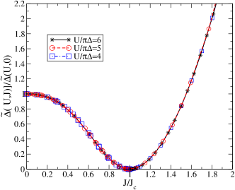
Figure 13: (Color online) A plot of $\tilde{\Delta}(U,J)/\tilde{\Delta}(U,0)$ as a function of $J/J_{c}$ for values of $U/\pi\Delta=4,5,6$. The results fall on a single curve indicating that this ratio becomes universal in the large $U$ regime.

IV.1 NRG Results for $U_{12}=0$, $J<J_{c}$

We first of all show results of a calculation for the renormalized parameters for the symmetric model. Results for $U/\pi\Delta=5$, which corresponds to the Kondo regime of the model, were given in earlier work NCH12 , so here we show results in a contrasting regime with $U=0$ in Fig. 5. Though $U=0$, a renormalized interaction $\tilde{U}$ is induced when the interaction $J$ is switched on; though rather small initially, it increases until $J\approx 0.7J_{c}$ and then falls to zero as $J\to J_{c}$. It can be seen that all the renormalized parameters, $\pi\tilde{\Delta}$, $\tilde{U}$ and $\tilde{J}$ tend to zero on the approach to the quantum critical point $J=J_{c}$. The ratios, $\tilde{U}/\pi\tilde{\Delta}$ and $\tilde{J}/\pi\tilde{\Delta}$, are shown in Fig. 6. The value of $\tilde{U}/\pi\tilde{\Delta}$ increases monotonically with increase of $J$ and tends to the strong coupling value $\tilde{U}/\pi\tilde{\Delta}=1$ on the approach to the critical point. The ratio $\tilde{J}/\pi\tilde{\Delta}$ also increases monotonically such that $\tilde{J}/\pi\tilde{\Delta}\to 2$ as $J\to J_{c}$. These results are in line with the RPT predictions in Eqn. (23).

We next look at a case where the two dots are hybridized differently to their respective baths so we have channel asymmetry. We take $V_{1}=2V_{2}$, which is such that $\Delta_{1}=4\Delta_{2}$, and take $\Delta_{2}=0.01$ and $U/\pi\Delta_{2}=6$. For $J=0$ we are dealing with two isolated Anderson models where the ratio of the renormalized energy scales of the two dots, $\tilde{\Delta}_{1}(J=0)/\tilde{\Delta}_{2}(J=0)=619.16$, are very different. In Fig. 7 we give plots of $\tilde{\Delta}_{1}(U,J)/\Delta_{1}(U,0)$, $\tilde{\Delta}_{2}(U,J)/\Delta_{2}(U,0)$, $\tilde{U}_{1}/\pi\Delta_{1}(U,0)$, $\tilde{U}_{2}/\pi\Delta_{2}(U,0)$, and $\tilde{J}/\pi(\tilde{\Delta}_{1}(U,0)\tilde{\Delta}_{2}(U,0))^{1/2}$ as a function of $J/J_{c}$. We see that $\tilde{U}_{2}=\pi\tilde{\Delta}_{2}(U,0)$ at $J=0$ showing that dot 2 is initially in the Kondo regime, but the ratio $\tilde{U}_{1}/\pi\tilde{\Delta}_{1}(U,0)<1$ so that initially dot 1 is not quite in the Kondo regime due to the larger value of the hybridization $\Delta_{1}(U,0)$. As $J$ is increased there is a transition at $J_{c}/\pi\Delta_{2}=0.1605$ where all the renormalized parameters tend to zero. The results imply that both $z_{1}\to 0$ and $z_{2}\to 0$, corresponding to a loss of the local quasiparticle weight at the Fermi level in both dots at the critical point.

To test the predictions based on the RPT given in the Eqn. (23) for this case, we plot the ratios of the renormalized parameters, $\tilde{J}/\pi\tilde{\Delta}_{1}$, $\tilde{J}/\pi\tilde{\Delta}_{2}$, $\tilde{U}_{1}/\pi\tilde{\Delta}_{1}$ $\tilde{U}_{2}/\pi\tilde{\Delta}_{2}$ and $\tilde{\Delta}_{2}/\tilde{\Delta}_{1}$ as a function of $J/J_{c}$ over the range $0.9<J/J_{c}<1$. Over this range we see that $\tilde{U}_{1}/\pi\tilde{\Delta}_{1}=\tilde{U}_{2}/\pi\tilde{\Delta}_{2}=1$, corresponding to strong coupling on both dots. Remarkably the ratio $\tilde{\Delta}_{2}/\tilde{\Delta}_{1}$, which was initially very small, $1/619.16\approx 0.001615$, approaches the strong coupling value 1 at the critical point. The two ratios, $\tilde{J}/\pi\tilde{\Delta}_{1}$ and $\tilde{J}/\pi\tilde{\Delta}_{2}$, converge to a common value 2 as $J\to J_{c}$. These results confirm the predictions given in Eqn. (23) for the case $U_{12}=0$. Furthermore, they show rather dramatically the emergence of channel symmetry as $J$ approaches the critical value $J_{c}$.

We found precisely similar results when we fixed the value of $J$ at $J/\pi\Delta_{2}=0.06$ and $U/\pi\Delta_{2}=6$, and increased the hybridization ratio $r=\Delta_{1}/\Delta_{2}$. A transition point was reached at $r=r_{c}=2.6732$, where all the renormalized parameters went to zero, and in the predicted ratios.

The transition in this model is remarkably robust and not only persists in cases where there is asymmetry between the two dots, but also away from particle-hole symmetry ZCSV06 . Before looking at an example of this type we consider how to calculate the renormalized parameters for the regime $J>J_{c}$.

IV.2 Extension of NRG results to $J>J_{c}$

IV.2.1 Particle-hole asymmetric case

For the regime $J>J_{c}$ there is a difference in the calculation of the renormalized parameters for the cases with and without particle-hole symmetry. In both cases the renormalized hybridization, which couples to dots to their respective conduction baths, $\tilde{V}_{\alpha}\to 0$ as $J\to J_{c}$ for $J<J_{c}$. In the particle-hole asymmetric case the renormalized hybridization re-emerges in the regime $J>J_{c}$, which means we can apply precisely the same analysis to the calculation of the renormalized parameters, $\tilde{\Delta}$ and $\tilde{\epsilon}_{d}$, using Eqn. (30), as described earlier. To see what happens as we pass through the transition we look at the results for a particular example.

In Fig. 9 we show the results deduced for the renormalized parameters over the range $0<J/J_{c}<1.2$ ($J_{c}/\pi\Delta=1.0884$) for the case with $U/\pi\Delta=0.5$ with $\epsilon_{d}/\pi\Delta=0.159$, where the level on the dot is initially above the Fermi level. It can be seen that all the renormalized parameters, $\tilde{\Delta}$, $\tilde{\epsilon}_{d}$, $\tilde{U}$ and $\tilde{J}$ go to zero as $J\to J_{c}$ both for $J<J_{c}$ and $J>J_{c}$. To learn in more detail what happens to the quantity $\tilde{\epsilon}_{d}$ through the quantum critical point we plot in Fig. 10 the product $\tilde{\epsilon}_{d}\tilde{\rho}(0)$ and $1/\tilde{\rho}(0)$ as a function of $J/J_{c}$. There is a discontinuity in $\tilde{\epsilon}_{d}\tilde{\rho}(0)$ at $J=J_{c}$ which reflects the fact that there is a discontinuous change in the phase shift $\delta_{\alpha}$ of $\pi/2$. From the Friedel sum rule (22) this implies that the total local occupation number in the ground state for $J>J_{c}$ has two more electrons than that for $J<J_{c}$. The local density of states $\rho(\omega)$ at each dot in the low frequency regime corresponds to $z\tilde{\rho}(\omega)$, and this is plotted in Fig. 11 for cases on either side of the transition, $J/J_{c}=0.98$ and $J/J_{c}=1.02$. The peak in $\tilde{\rho}(\omega)$ has shifted from just above the Fermi level for $J/J_{c}=0.98$ to below for $J/J_{c}=1.02$. In the inset of Fig. 11 $\rho(0)$ ($=z\tilde{\rho}(0)$) is plotted as a function of $J/J_{c}$. It can be seen that as the value of $J$ increases through the transition there is a sudden loss of spectral weight at the Fermi level but there is finite spectral weight on both sides of the transition.

To check the RPT predictions given in Eqn. (23) we have plotted $\tilde{U}\tilde{\rho}(0)$ and $\tilde{J}\tilde{\rho}(0)$ in Fig. 12. It can be seen that $\tilde{U}\tilde{\rho}(0)\to 1$ and $\tilde{J}\tilde{\rho}(0)\to 2$ as $J\to J_{c}$ on both sides of the quantum critical point in agreement with the RPT prediction.

IV.2.2 Particle-hole symmetric case

The case of particle-hole symmetry differs from the case we have just considered as the renormalized hybridization parameter $\tilde{V}_{\alpha}$, calculated from the NRG, does not just go to zero as $J\to J_{c}$ for $J<J_{c}$ but remains equal to zero for all $J>J_{c}$. This implies that we lose all the spectral weight at the transition for the particle-hole symmetric case, and not just some of the spectral weight as was the case with particle-hole asymmetry. At the fixed point for $J>J_{c}$ the two dots are decoupled from the conduction electrons on the lowest energy scale. We know, however, for $J>J_{c}$ the low energy behavior still corresponds to a Fermi liquid. We conjecture that this Fermi liquid can be described by a similar set of renormalized parameters and that the equations for the susceptibility and low energy behavior are still valid. However, this needs to be clarified.

The fact that $z\to 0$ implies that the derivative of the the self-energy in the impurity Green’s function, $\Sigma^{\prime}(\omega)$, diverges at $\omega=0$ such that this self-energy develops a singularity as $J\to J_{c}$. The fact that $z=0$ for $J>J_{c}$ means that that this singularity persists in the regime $J>J_{c}$ and the analysis outlined in the previous section breaks down. To consider this situation in more detail, we sum over $k$ and $k^{\prime}$ in Eqn. (20) to obtain an equation for the Green’s function on the first site of the conduction electron chain in the NRG calculation which we denote by $G_{0,\alpha,\sigma}(\omega)$,

$$G_{0,\alpha,\sigma}(\omega)=G^{(0)}_{0,\alpha,\sigma}(\omega)+G^{(0)}_{0,\alpha,\sigma}(\omega)V_{\alpha}^{2}G_{d,\alpha,\sigma}(\omega)G^{(0)}_{0,\alpha,\sigma}(\omega).$$ (31)

If we take the conduction band in the wide band limit, $V_{\alpha}^{2}G^{(0)}_{0,\alpha,\sigma}(\omega)=-i\pi\Delta_{\alpha}$, this equation becomes

$$G_{0,\alpha,\sigma}(\omega)=G^{(0)}_{0,\alpha,\sigma}(\omega)\left(1-i\Delta G_{d,\alpha,\sigma}(\omega)\right).$$ (32)

If we introduce a self-energy $\Sigma^{0}_{\alpha,\sigma}(\omega)$ for the Green’s function for the first site on the $\alpha$ conduction electron chain, which will also include the effect of switching on the hybridization term, Eqn. (32) becomes

$${1+i\rho_{c}\Sigma^{0}_{\alpha,\sigma}(\omega)}={1\over 1-i\Delta G_{d,\alpha,\sigma}(\omega)}.$$ (33)

For $J<J_{c}$ the self-energies on the dot are non-singular and from the Friedel sum rule $\epsilon_{d}+\Sigma_{\alpha}(0)=0$ corresponding to a phase shift $\delta_{\alpha}=\pi/2$. We then have $G_{d,\alpha,\sigma}(0)=1/i\Delta_{\alpha}$ for the case of particle-hole symmetry and hence from Eqns. (32) and (33) the Green’s function on the first site of the conduction chain is zero, $G_{0,\alpha,\sigma}(0)=0$, and the self-energy $\Sigma^{0}_{\alpha,\sigma}(\omega)$ diverges at $\omega=0$.

For $J>J_{c}$, however, the dot self-energy develops a divergence at $\omega=0$, such that the dot Green’s function vanishes for $\omega=0$, and we get a phase shift $\delta_{\alpha}=0$. The self-energy for the first conduction site is now non-singular and from Eqn. (33), $\Sigma^{0}_{\alpha,\sigma}(0)=0$. We can then develop a renormalized perturbation approach and analysis of the low energy NRG fixed point with the first conduction site playing the role of an effective dot. We should, therefore, be able to describe the Fermi liquid behavior for $J>J_{c}$ in terms of renormalized parameters associated with the first site on the impurity conduction electron chain.

For $J<J_{c}$ we determine the renormalized parameters $\tilde{\epsilon}_{d}$ and $\tilde{V}$ by requiring the lowest energy particle and hole excitations of the interacting systems to correspond to poles of the impurity quasiparticle Green’s function. For $J>J_{c}$ we can adopt the same procedure but replacing the Green’s function of the impurity site by that for the first conduction electron site, so that parameters for $\tilde{\epsilon}_{0}$ and $\tilde{V}_{0}$ are required to correspond to solutions of the equation,

$$E_{p/h,\alpha}(N)-\tilde{\epsilon}_{0}-\tilde{V}_{0}^{2}G_{1,\alpha,\sigma}^{(0)}(E_{p/h,\alpha}(N))=0,$$ (34)

where $G_{1,\alpha,\sigma}^{(0)}(\omega)$ is given by Eq. (28). The local quasiparticle interaction terms, $\tilde{U}$, $\tilde{J}$ and $\tilde{U}_{12}$, can then be calculated as in the case $J<J_{c}$.

As the effective impurities now correspond to the first site on the conduction electron chain for each channel, there are a some modifications to the analysis used for $J<J_{c}$. The density of states of the conduction electron chain which now starts at the second conduction site is modified, which affects the calculation of the effective hybridization width $\Delta_{0}=\pi|V_{0}|^{2}\rho_{c}$, where $\rho_{c}$ is the density of conduction states at the Fermi level. The factor $A_{\Lambda}$, which relates the hybridization width of the discretized model to the continuum model, also changes. These two effects can be combined into a single additional factor $B_{\Lambda}$ so that the hybridization width $\Delta_{0}$ for the continuum model is calculated from $\Delta_{0}=\pi|V_{0}|^{2}/2A_{\Lambda}B_{\Lambda}D$. The value of $B_{\Lambda}$ was estimated from the result for the isolated Anderson model ($J=0$) for $U/\pi\Delta\gg 1$, $\tilde{U}/\pi\tilde{\Delta}\to 1$, which for a discretization parameter $\Lambda=6$, gave the value $B_{6}=2.2373$.

In the limit $J\to\infty$ the two impurities are entirely decoupled from the conduction electrons. This is reflected in the NRG results for the renormalized parameter $\tilde{V}_{0}$, which in this limit give $\tilde{V}_{0}\to\Lambda^{-1/2}\xi_{1}$, which is the value for the free NRG conduction chain. The calculation of the impurity susceptibility using the RPT expression with $\tilde{\Delta}_{0}$ includes this extra conduction electron contribution. However, this correction is negligible except in the regime when $J/J_{c}$ is very large and it is not necessary to take it into account.

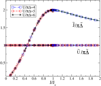
Figure 14: (Color online)A plot of $\tilde{U}/\pi\tilde{\Delta}$ and $\tilde{J}/\pi\tilde{\Delta}$, as a function of $J/J_{c}$ for $U/\pi\Delta=4,5,6$.

IV.3 NRG results for $J\neq 0$, $U_{12}=0$

We now consider the channel and particle-hole symmetric model taking $V_{1}=V_{2}$ so we can drop the channel index $\alpha$. We extend the results for the renormalized parameters to include the regime $J>J_{c}$. We restrict attention first of all to the strong correlation regime $U/\pi\Delta\gg 3$ for different values of $U$. In Fig. 13 we plot the results for the ratio $\tilde{\Delta}(U,J)/\tilde{\Delta}(U,0)$ as a function of $J/J_{c}$ for $U/\pi\Delta=4,5,6$ over the range $0<J/J_{c}<2$. It can be seen that, though the values of $J_{c}$ vary significantly, all three results fall on a single curve indicating universal behavior in this regime. We have dropped the index on $\Delta_{0}$ and $\tilde{\Delta}_{0}$ for the regime $J>J_{c}$, to define a continuous function $\tilde{\Delta}$ through the transition point. With the definition of the Kondo temperature $T_{\rm K}$, $\pi\tilde{\Delta}(U,0)=4T_{\rm K}$ and the energy scale $T^{*}(U,J)$, $\pi\tilde{\Delta}(U,J)=4T^{*}$ we now have a single energy scale over the range $0<J/J_{c}<2$ such that in the strong correlation regime,

$$T^{*}=T_{\rm K}F(J/J_{c}),$$ (35)

where the function $F(J/J_{c})$ is independent of $U$ for $U/\pi\Delta\gg 1$, such that $F(0)=1$ and $F(1)=0$. We also have $J_{c}=1.378T_{\rm K}$ in this regime, so Eqn. (35) can be re-expressed in the form, $T^{*}=T_{\rm K}F(0.726J/T_{\rm K})$.

In Fig. 14 we plot the ratios $\tilde{U}/\pi\tilde{\Delta}$ and $\tilde{J}/\pi\tilde{\Delta}$, for $U/\pi\Delta=4,5,6$ over the same range. All the values for $\tilde{U}/\pi\tilde{\Delta}$ fall on the same line $\tilde{U}/\pi\tilde{\Delta}=1$ corresponding to the strong coupling limit. The values of $\tilde{J}/\pi\tilde{\Delta}$ also all lie on a single curve. Hence, using Eqn. (35), in this regime we have

$${\tilde{J}}=4T^{*}f({J/J_{c}}),$$ (36)

where $f(J/J_{c})$ is a universal function such that $f(0)=0$ and $f(1)=2$. As from Eqn. (35) $T^{*}$ is a universal function of $J$ and $T_{\rm K}$ then Eqn. (36) can be re-expressed as ${\tilde{J}}=T_{\rm K}\bar{f}({0.726J/T_{\rm K}})$, where $\bar{f}(J/J_{c})$ is a universal function such that $\bar{f}(0)=0$ and $\bar{f}(1)=0$.

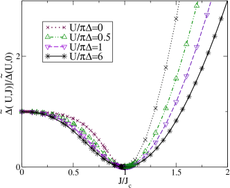
Figure 15: (Color online) A plot of $\tilde{\Delta}(U,J)/\tilde{\Delta}(U,0)$ as a function of $J/J_{c}$ for values of $U/\pi\tilde{\Delta}=0,0.5,1,6$.

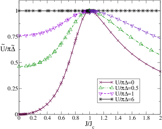
Figure 16: (Color online) A plot of $\tilde{U}/\pi\tilde{\Delta}$, as a function of $J/J_{c}$ for $U/\pi\Delta=0,0.5,1,6$.

The universality found in the Kondo regime $U/\pi\Delta\gg 1$ no longer holds for smaller values of $U$ as can be seen in Fig. 15 where we give results for the ratio of $\tilde{\Delta}(U,J)/\tilde{\Delta}(U,0)$ over the range $0<J/J_{c}<2$ for values of $U/\pi\Delta=0,0.5,1,2,6$ as a function of $J/J_{c}$. It can be seen that they all qualitatively behave in a similar way, but for smaller values of $U/\pi\Delta$ the results do not lie on the same curve.

In Figs. 16 and 17 we give the corresponding plot for the ratios $\tilde{U}/\pi\tilde{\Delta}$ and $\tilde{J}/\pi\tilde{\Delta}$. There is no universality except in the approach to the critical point where $\tilde{U}/\pi\tilde{\Delta}\to 1$ and $\tilde{J}/\pi\tilde{\Delta}\to 2$ in all cases in line with the predictions in Eqn. (23).

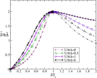
Figure 17: (Color online) A plot of $\tilde{J}/\pi\tilde{\Delta}$, as a function of $J/J_{c}$ for $U/\pi\Delta=0,0.5,1,6$.

The factors $\tilde{\eta}_{s}$ and $\tilde{\eta}_{c}$ in the expressions for the spin and charge susceptibilities reflect the effect of the interaction between the quasiparticles in enhancing or suppressing the corresponding fluctuations. For the single impurity Anderson model $\tilde{\eta}_{s}$ is better known as the Wilson ratio and in the strong coupling regime has the value 2, enhanced over that for non-interacting quasiparticles where the value would be 1. In Fig. 18 we plot the values of $\tilde{\eta}_{s}$ for $U/\pi\Delta=4,5,6$ as a function of $J/J_{c}$. We see that there is a universal curve in this regime which falls from the value 2 for the isolated impurities to zero at the critical point. In Fig. 19 the values of $\tilde{\eta}_{s}$ are plotted as a function of $J/J_{c}$ for $U/\pi\Delta=0,0.5,1,4$. There is non-universal behavior in the regime, though the results for $U/\pi\Delta=4$ correspond to the universal curve for the strong coupling limit.

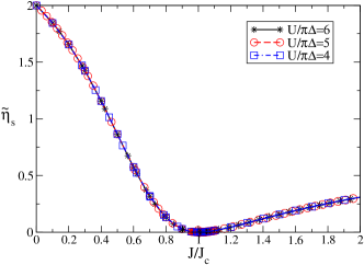
Figure 18: (Color online) A plot of the Wilson ratio $\tilde{\eta}_{s}$ as a function of $J/J_{c}$ for $U/\pi\Delta=4,5,6$ for $\pi\Delta=0.01$.

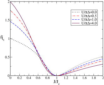
Figure 19: (Color online) A plot of $\tilde{\eta}_{s}$, as a function of $J/J_{c}$ for $U/\pi\Delta=0,0.5,1,4$ for $\pi\Delta=0.01$.

The values of $\tilde{\eta}_{c}$ for $U/\pi\Delta=0,0.5,1$ are shown in Fig. 20. For $U=0$ and $J=0$ the value is 1 corresponding to a non-interacting system and then, as $J$ is increased, progressively reduces to zero (corresponding to the Kondo limit) as $J\to J_{c}$. For the larger values of $U$, $\tilde{\eta}_{c}$ is already reduced at $J=0$, due to the on-site interaction $U$, and is then further reduced to zero as the exchange interaction increases to the critical value. For $U/\pi\Delta>3.5$, $\tilde{\eta}_{c}\approx 0$ as the charge fluctuations are almost completely suppressed for all values of $J$ in this range.

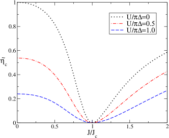
Figure 20: (Color online) A plot of $\tilde{\eta}_{c}$, as a function of $J/J_{c}$ for $U/\pi\Delta=0,0.5,1$ for $\pi\Delta=0.01$.

All the expressions given in the previous section apply equally well to the situation with a ferromagnetic exchange $J<0$. In figure 21 we show the values of $\tilde{\eta}_{s}$ as a function of $J/\pi\Delta$ extended to the ferromagnetic range for $U/\pi\Delta=5$, where it extrapolates to the expected value $8/3$.

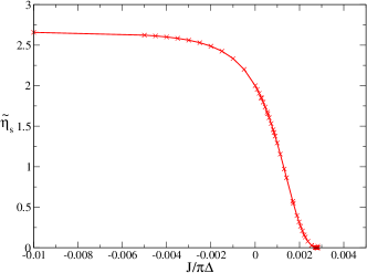
Figure 21: (Color online) A plot of $\tilde{\eta}_{s}$ (Wilson ratio) as a function of $J/\pi\Delta$, including the ferromagnetic range, for $U/\pi\Delta=5$ for $\pi\Delta=0.01$.

IV.4 Results for $U_{12}<U_{12}^{c}$, $J=0$

The transition to a locally charge ordered state in the model with a finite interaction $U_{12}$ ($J=0$) has been studied in detail by Galpin et al GLK06 . Here we throw further light on this transition by calculating the renormalized parameters. In particular we test the RPT conjecture of the emergence of a single energy scale on the approach to the QCP and the predictions given in Eqn. (24).

In Fig. 22 we give results for the ratio $\tilde{\Delta}/\Delta$ as a function of $U_{12}/U$ for the case $U/\pi\Delta=5$. Over the range $U_{12}/U<0.8$ there is a slow steady increase in $\tilde{\Delta}$ with increasing $U_{12}$. There is then a rapid increase due to fluctuations of charge between the two dots and $\tilde{\Delta}$ reaches a maximum at the SU(4) point $U_{12}=U$, and an extremely rapid fall off beyond this point to a QCP at $U_{12}/U=1.028$. In Fig. 23 the corresponding results for the renormalized parameter ratios, $\tilde{U}/\pi\tilde{\Delta}$ and $\tilde{U}_{12}/\pi\tilde{\Delta}$, are shown as a function of $U_{12}/U$ over the same range. Over the range $U_{12}/U<0.9$ these ratios differ very little from the values for the Anderson model in the Kondo regime, $\tilde{U}/\pi\tilde{\Delta}=1$ and $\tilde{U}_{12}/\pi\tilde{\Delta}=0$. Beyond this point there is a rapid change and the two curves cross at the SU(4) point where $\tilde{U}/\pi\tilde{\Delta}=\tilde{U}_{12}/\pi\tilde{\Delta}={1/3}$. This result follows from the RPT equations for the susceptibility from the condition that the uniform charge susceptibility $\chi_{c}$ is so small, due to the large value of $U$, that it can be equated to zero. Beyond the SU(4) point the ratios rapidly approach the values predicted in Eqn. (24) on the approach to the QCP, $\tilde{U}/\pi\tilde{\Delta}=-1$ and $\tilde{U}_{12}/\pi\tilde{\Delta}=1$.

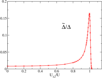
Figure 22: (Color online) A plot of $\tilde{\Delta}/\Delta$ as a function of $U_{12}/U$ for $U/\pi\Delta=5$.

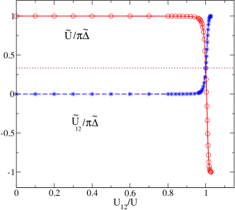
Figure 23: (Color online) A plot of $\tilde{U}/\pi\tilde{\Delta}$ (circles) and $\tilde{U}_{12}/\pi\tilde{\Delta}$ (stars) as a function of $U_{12}/U$ for $U/\pi\Delta=5$. The dotted line which passes through the SU(4) point corresponds to $\tilde{U}_{12}/\pi\tilde{\Delta}=\tilde{U}/\pi\tilde{\Delta}=1/3$.

The question arises as to what happens for smaller values of $U$ and in particular the case $U=0$. This is addressed in Fig. 24 which shows a plot of $\tilde{U}/\pi\tilde{\Delta}$ as a function of $U_{12}/U_{12}^{c}$ for values of $U/\pi\Delta=0,0.5,1,2,3,5$. We see that in all cases $\tilde{U}/\pi\tilde{\Delta}\to-1$ as $U_{12}\to U_{12}^{c}$, though less rapidly the smaller the value of $U$. This also holds for the case $U=0$ so that switching on the interaction term $U_{12}$ induces an onsite effective interaction $\tilde{U}$ in the quasiparticle Hamiltonian.

The corresponding curves for the ratio $\tilde{U}_{12}/\pi\tilde{\Delta}$ as a function of $U_{12}/U_{12}^{c}$ are shown in Fig. 25. We see that it this case all the curves approach the predicted value $\tilde{U}_{12}/\pi\tilde{\Delta}\to 1$ as $U_{12}\to U_{12}^{c}$, though much less rapidly for the smaller values of $U$.

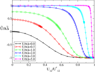
Figure 24: (Color online) Plots of $\tilde{U}/\pi\tilde{\Delta}$ as a function of $U_{12}/U_{12}^{c}$ for values of $U/\pi\Delta=0,0.5,1,2,3,5$, $J=0$.

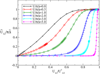
Figure 25: (Color online) Plots of $\tilde{U}_{12}/\pi\tilde{\Delta}$ as a function of $U_{12}/U_{12}^{c}$ for values of $U/\pi\Delta=0,0.5,1,2,3,5$, $J=0$.

IV.5 NRG results for $J\neq 0$ and $U_{12}\neq 0$

To complete the check on the predictions in Eqns. (23) and (24) we look at some examples with finite values of both $J$ and $U_{12}$. We look first at a case with $U/\pi\Delta=U_{12}/\pi\Delta=5$ over a range of values of $J$ through the critical point $J_{c}=0.09015\pi\Delta$. This corresponds to moving along a vertical line in Fig. 4 with $U_{12}/D=0.05$. The results for the renormalized parameter ratios, $\tilde{J}/\pi\tilde{\Delta}$, $\tilde{U}/\pi\tilde{\Delta}$ and $\tilde{U}_{12}/\pi\tilde{\Delta}$ are shown in Fig. 26. The results include the regime with ferromagnetic coupling $J<0$, and it can be seen that as the ferromagnetic coupling increases $\tilde{U}/\pi\Delta$ approaches the value 1 and $\tilde{J}/\pi\tilde{\Delta}$ the value $-2/3$ as expected in the regime where the channel and charge fluctuations are suppressed. The value of $U_{12}/\pi\tilde{\Delta}$ is small in this limit but increases as the ferromagnetic coupling is reduced. At $J=0$ there is an SU(4) point where the curves for $\tilde{U}/\pi\tilde{\Delta}$ and $\tilde{U}_{12}/\pi\tilde{\Delta}$ meet at a common value $1/3$, and $\tilde{J}=0$. As $J$ is increased from $J=0$ the curves for $\tilde{J}/\pi\tilde{\Delta}$ and $\tilde{U}/\pi\tilde{\Delta}$ increase to a maximum at the transition point $J=J_{c}$, where they reach the values 2 and 1, respectively. At this point $\tilde{U}_{12}/\pi\tilde{\Delta}=0$ in line with the general prediction in Eqn. (23). This means that switching on and increasing the value of $J$ have the effect of cancelling out the $\tilde{U}_{12}/\pi\Delta$ ratio which is finite for $J=0$, and reducing it to zero as $J\to J_{c}$. For $J>J_{c}$, the values of $\tilde{J}/\pi\tilde{\Delta}$, $\tilde{U}/\pi\tilde{\Delta}$ fall off significantly with increase of $J$ and $\tilde{U}_{12}/\pi\tilde{\Delta}$ has a slow increase.

In Fig. 27 we plot the same ratios of the renormalized parameters but in this case we take value $U_{12}/\pi\Delta=5.2$. We take a range of values of $J$ corresponding to moving along a vertical line in Fig. 4, $U_{12}/D=0.052$. We see in this case the line passes through three QCPs. For the ferromagnetic regime where $(J-J_{c})/J_{c}<-6$, the spin and inter-dot fluctuations are suppressed and the ratios take on the expected values, $\tilde{U}/\pi\tilde{\Delta}=1$, $\tilde{J}/\pi\tilde{\Delta}=-2/3$ and $\tilde{U}_{12}/\pi\tilde{\Delta}=0$. Around $(J-J_{c})/J_{c}\sim-4$ there is a rapid change over as the values move to $\tilde{U}/\pi\tilde{\Delta}=-1$, $\tilde{J}/\pi\tilde{\Delta}=0$ and $\tilde{U}_{12}/\pi\tilde{\Delta}=1$ on the approach to the local charge order transition at $(J-J_{c})/J_{c}\approx-2.1$. When $(J-J_{c})/J_{c}\approx-0.25$ the system emerges from the charge ordered state, with the same set of ratios, but as $J\to J_{c}$ there is a rapid change of the ratios of the renormalized parameters to the ratios, $\tilde{U}/\pi\tilde{\Delta}=1$, $\tilde{J}/\pi\tilde{\Delta}=2$ and $\tilde{U}_{12}/\pi\tilde{\Delta}=0$ on the approach to the transition to the local singlet state. There is a rapid decrease in $\tilde{U}/\pi\tilde{\Delta}$, $\tilde{J}/\pi\tilde{\Delta}$ and an increase in the ratio $\tilde{U}_{12}/\pi\tilde{\Delta}$. For $(J-J_{c})/J_{c}>0.25$ there is a slow fall off with increase of $J$ for all three ratios.

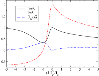
Figure 26: (Color online) A plot of the renormalized parameter ratios, $\tilde{J}/\pi\tilde{\Delta}$, $\tilde{U}/\pi\tilde{\Delta}$ and $\tilde{U}_{12}/\pi\tilde{\Delta}$ as a function of $(J-J_{c})/J_{c}$ where $J_{c}=0.09015\pi\Delta$ for $U/\pi\Delta=U_{12}/\pi\Delta=5$. As $J$ is increased there is an SU(4) point at $J=0$ where $\tilde{U}/\pi\tilde{\Delta}=\tilde{U}_{12}/\pi\tilde{\Delta}=1/3$ and $\tilde{J}=0$ followed by a transition at $J=J_{c}$ from the Fermi liquid phase $J<J_{c}$ to the second Fermi liquid phase $J>J_{c}$.

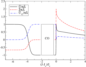
Figure 27: (Color online) A plot of the renormalized parameter ratios, $\tilde{J}/\pi\tilde{\Delta}$, $\tilde{U}/\pi\tilde{\Delta}$ and $\tilde{U}_{12}/\pi\tilde{\Delta}$ as a function of $(J-J_{c})/J_{c}$ where $J_{c}=0.27228\pi\Delta$ for $U/\pi\Delta=5$, $U_{12}/\pi\Delta=5.2$. As $J$ is increased there is first transition from a Fermi liquid phase $J<J_{c}$ to a local charged ordered regime indicated by the box (CO) followed by a return to the Fermi liquid phase $J<J_{c}$ and then a transition to the second Fermi liquid phase $J>J_{c}$.

IV.6 The case $U_{12}=U+3J/2$

There is a special line in the phase diagram shown in Fig. 4, corresponding to $U_{12}=U+3J/2$ along which there appears to be no transition. With this set of parameters, and a ferromagnetic exchange coupling ($J<0$), the model corresponds to a model introduced by Yoshimori Yos76 to describe a single impurity with an $n$-fold degenerate orbital for the case $n=2$. The exchange interaction $J$ in this context corresponds to a Hund’s rule term. The model in the ferromagnetic regime was used to calculate the orbital susceptibilityNCH10s ; NCH10a for a two-fold degenerate impurity with a Hund’s rule interaction $J$, where the orbital susceptibility is given by

$$\chi_{orb}={\mu_{\rm B}^{2}\eta_{orb}\tilde{\rho}(0)\over 4},\quad\eta_{orb}=1+(\tilde{U}+3\tilde{J})\tilde{\rho}(0).$$ (37)

As the value of $|J|$ is increased in the ferromagnetic range the orbital fluctuations are suppressed and the two local spins are coupled to give an effective spin 1. When $\tilde{\eta}_{\rm orb}\sim 0$ from Eq. (37) we find the value, $|\tilde{J}|=2\pi\tilde{\Delta}/3$. The value $\tilde{\eta}_{s}$ approaches $\tilde{\eta}_{s}=8/3$, as expected for the Wilson ratio for a two channel Kondo model.

We have previously calculated the renormalized parameters for this model, both for the particle-hole symmetric and antisymmetric models, for a ferromagnetic coupling NCH10s ; NCH10a . It is interesting to check here what happens in the antiferromagnetic case. The lack of a transition is likely to be due to the fact that for the isolated dots at half filling the gain in energy in forming a local singlet $-3J/2$ is compensated by an equal and opposite term from the $J$-dependence of the $U_{12}$ term. We look at the results for the renormalized parameters in detail.

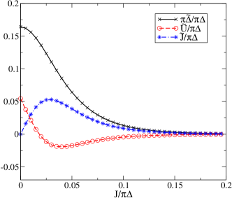
Figure 28: (Color online) A plot of the renormalized parameters,$\pi\tilde{\Delta}/\pi\Delta$, $\tilde{U}/\pi\Delta$ and $\tilde{J}/\pi\Delta$ as a function of $J/\pi\Delta$ for $U/\pi\Delta=5$, $U_{12}=U+3J/2$.

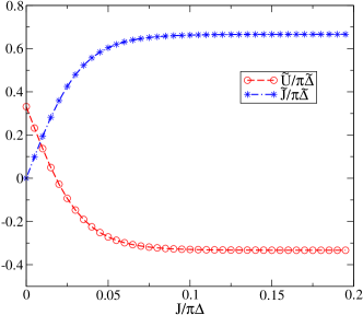
Figure 29: (Color online) A plot of ratios of the renormalized parameters, $\tilde{U}/\pi\tilde{\Delta}$ and $\tilde{J}/\pi\tilde{\Delta}$ as a function of $J/\pi\Delta$ for $U/\pi\Delta=5$, $U_{12}=U+3J/2$.

In Fig. 28 we plot the renormalized parameters $\pi\tilde{\Delta}/\pi\Delta$, $\tilde{U}/\pi\Delta$ and $\tilde{J}/\pi\Delta$ as a function of $J/\pi\Delta$ over an antiferromagnetic range of $J$ for $U/\pi\Delta=5$. The value of $\tilde{\Delta}$, and consequently the quasiparticle weight factor $z$, decreases monotonically to very small values for large $J$ without any evidence of a transition. Somewhat surprisingly in this case the value of $\tilde{U}/\pi\Delta$ decreases and becomes negative with increase of $J$.

In Fig. 29 we plot that ratios $\tilde{U}/\pi\tilde{\Delta}$ and $\tilde{J}/\pi\tilde{\Delta}$ as a function of $J/\pi\Delta$. For $J=0$, $\tilde{U}/\pi\tilde{\Delta}=1/3$, which is predicted from the condition that the $\tilde{\eta}_{c}\sim 0$ due to the large value of $U/\pi\Delta$ which suppresses the charge susceptibility. For large $J$, $\tilde{U}/\pi\tilde{\Delta}\to-1/3$ and $\tilde{J}/\pi\tilde{\Delta}\to 2/3$, so there is a single energy scale for large values of $J$. These results are in line with predictions based on the fact that for large $U$ and large $J$ both the charge and spin susceptibilities are suppressed so $\tilde{\eta}_{c}\to 0$ and $\tilde{\eta}_{s}\to 0$. From Eq. (17) the condition $\tilde{\eta}_{c}\to 0$ we find $3(\tilde{U}+\tilde{J})=\pi\tilde{\Delta}$. Using this result in the expressions for $\tilde{\eta}_{s}$ and $\tilde{\eta}_{orb}$ we find

$$\tilde{\eta}_{s}={4\over 3}-{2\tilde{J}\over\pi\tilde{\Delta}},\quad\tilde{\eta}_{orb}={4\over 3}+{2\tilde{J}\over\pi\tilde{\Delta}}.$$ (38)

From the condition $\tilde{\eta}_{s}\to 0$, using Eq. (17), we find $\tilde{J}/\pi\tilde{\Delta}\to 2/3$. When this result is substituted into the earlier condition, $3(\tilde{U}+\tilde{J})=\pi\tilde{\Delta}$, we find $\tilde{U}/\pi\tilde{\Delta}\to-1/3$ in this limit, and $\tilde{\eta}_{orb}\to 8/3$.

From earlier results for this model in the ferromagnetic range NCH10s , when $|J|$ was large such that the orbital susceptibility was suppressed we found $\tilde{J}/\pi\tilde{\Delta}\to-2/3$ and $\tilde{\eta}_{s}\to 8/3$, which suggests from Eq. (38) the relation $\tilde{\eta}_{s}\leftrightarrow\tilde{\eta}_{orb}$ if $\tilde{J}/\pi\tilde{\Delta}\leftrightarrow-\tilde{J}/\pi\tilde{\Delta}$ under the sign change $J\to-J$. In Fig. 30 we plot the values of $\tilde{\eta}_{s}$, $\tilde{\eta}_{orb}$ and $\tilde{\eta}_{c}$ as a function of $J/\tilde{\Delta}(5,0)$ for $U/\pi\Delta=5$. The results show that there is an approximate symmetry $\tilde{\eta}_{s}\leftrightarrow\tilde{\eta}_{orb}$ as $J\leftrightarrow-J$, but it is not precise for values in the intermediate range of $|J|$ where the differences, though small, are greater than any that might arise from the estimated errors in the calculation of the renormalized parameters.

In the antiferromagnetic regime there is still the tendency for the impurity spins to be screened more locally as $J$ is increased. This can be seen in the plot of $\chi_{s}$ shown in Fig. 31. The value of $\chi_{s}$ decreases monotonically as $J/\pi\Delta$ increases to a value $J/\pi\Delta\sim 0.15$. After that point there appears to be a slight upturn, but no real significance can be attached to this as it involves the product of a quantity tending to zero $\tilde{\eta}_{s}$ and a diverging quantity $1/z\pi\Delta$ as $z\to 0$, and numerical errors start becoming significant when $z$ becomes very small. Though we get no transition in this case it does not correspond to the category described by Affleck et al. ALJ95 , where the phase shift $\delta$ decreases with increases of $J$. For the whole range of $J$ the phase shift remains at the value $\delta=\pi/2$. It would appear that provided the Friedel sum rule applies for particle-hole symmetry $\langle n_{d,\alpha,\sigma}\rangle=1/2$ and if Eq. $\epsilon_{d}+\Sigma(0)=0$, we always have a phase shift $\delta=\pi/2$, so we cannot have a continuous crossover from $\delta=\pi/2$ to $\delta=0$. Either there is no transition and $\delta=\pi/2$ for all $J$ or the self-energy develops a singularity at $\omega=0$, with a breakdown of the Friedel sum rule, and a sharp transition to a state with $\delta=0$.

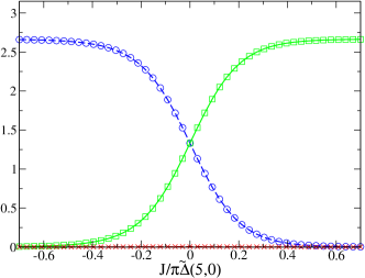
Figure 30: (Color online) A plot of $\tilde{\eta}_{s}$ (circles), $\tilde{\eta}_{orb}$ (squares) and $\tilde{\eta}_{c}$ (crosses) as a function of $J/\pi\tilde{\Delta}(5,0)$ for $U_{12}=U+3J/2$, $U/\pi\Delta=5$.

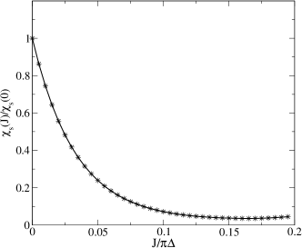
Figure 31: (Color online) A plot of $\chi_{s}(J)/\chi_{s}(0)$ as a function of $J/\pi\tilde{\Delta}$ for $U_{12}=U+3J/2$, $U/\pi\Delta=5$.

V Conclusions

We have examined the low energy behavior in the Fermi liquid regime of a model that has two types of quantum critical points. The thermodynamic and dynamic response functions in this regime can be expressed in terms of a limited number of renormalized parameters, $\tilde{\Delta}$, $\tilde{U}$, $\tilde{J}$ and $\tilde{U}_{12}$, which we can calculate accurately from an analysis of the NRG low energy fixed point. Once these have been determined they can then be substituted into the relevant RPT formulae. The fact that certain susceptibilities remain finite at the transition, where the quasiparticle weight $z\to 0$, gives enough equations to predict the dimensionless parameters, $\tilde{U}\tilde{\rho}(0)$, $\tilde{J}\tilde{\rho}(0)$ and $\tilde{U}_{12}\tilde{\rho}(0)$ in the Fermi liquid region on the approach to the critical point. These predictions have been confirmed from the NRG results for both types of transition, including situations away from particle-hole symmetry, and dot asymmetry in the case of the transition at $J=J_{c}$. As these dimensionless parameters are universal on the approach to the critical points, the quasiparticle interactions, $\tilde{U}$, $\tilde{J}$ and $\tilde{U}_{12}$, can all be expressed in terms of a single energy scale $T^{*}=1/4\tilde{\rho}(0)$, where $T^{*}\to 0$ at the critical point.

In this paper we have not examined the finite temperature non-Fermi liquid regime in the region of the critical point at $J=J_{c}$, but in our NRG results we found the same higher energy non-Fermi liquid fixed point as observed in previous calculations for the two impurity Kondo modelALJ95 . Those results were explained by Affleck and LudwigAL92 ; ALJ95 using conformal field theory. More recent work has clarified with the relation between this transition and the non-Fermi liquid fixed point of the two channel Kondo model. A recent paper of Sela and MitchellMS12 has addressed the crossover as a function of temperature between the Fermi liquid and non-Fermi liquid regimes. It would be interesting to examine this crossover in terms of renormalized parameters using the approach which was developed and applied to the two channel Kondo modelBHZ97 ; BBHZ99 .

It has proved difficult to probe the quantum critical point of the two dot/impurity model experimentally. The problem is that in any experimental set up there will be in addition to the interdot/impurity interaction a direct or indirect hybridization term. This was the case in the recent experimental work on a two impurity system which consisted of a cobalt ion on a STM point and interacting with a second cobalt ion on a metal surface. The hybridization term destroys the critical point. Nevertheless it would be interesting to generalize the model used here to model this experimental system, to see if the quantum critical behavior could be observed due to the presence of a higher energy non-Fermi liquid fixed point, as was done in the case of the two channel Kondo model.

The quantum critical points studied here are for impurity models and cannot be applied directly to the experimental results on quantum critical behavior observed in lattice heavy fermion systems. However, certain features found may be universal and apply to a general class quantum critical points. For example, the fact that on the approach to the quantum critical points all the quasiparticle interactions could be expressed in terms of a single energy scale $T^{*}$ means that any dynamic response function $\chi(\omega)$ should take the form $\chi(\omega)=F(\omega/T^{*},T/T^{*})$. At the critical point where $T^{*}\to 0$ we would then expect a form, $\chi(\omega)=T^{a}f(\omega/T)$, or $\omega/T$ scaling which has been observed at the several heavy fermion critical points, such as in YbRu₂Si₂Pfau2012 . The quantum critical point induced in YbRu₂Si₂ by suppressing the antiferromagnetic order with a magnetic field and has been interpreted as a Kondo breakdownSS10 ; CPSR01 , where the loss of the f-electron states at the Fermi surface results in a change in volume of the Fermi surface at the quantum critical point. A schematic sketch is given Fig. 4 in the paper of Pfau et al. Pfau2012 of the evolution of the quasiparticle weight factor $z$ across such a quantum critical point. At the critical point $J=J_{c}$ in our calculations in the particle-hole symmetric case there is a similar Kondo breakdown because the Kondo resonance at the Fermi level for $J<J_{c}$ collapses at $J=J_{c}$ and there are no impurity/dot f-states at the Fermi level for $J>J_{c}$. In Fig. 13 we have precise results for this evolution of the quasiparticle weight factor $z$ for the Kondo collapse in a two impurity model (note that for comparison with the sketch for YbRu₂Si₂, the range $J>J_{c}$ corresponds to the small Fermi surface and $J<J_{c}$ to the large one).

Acknowledgment

We thank Akira Oguri and Johannes Bauer for helpful discussions. Two of us (DJGC and ACH) thank the EPRSC for support (Grant No. EP/G032181/1). The numerical calculations were partly carried out at the Yukawa Institute Computer Facility.

VI Appendix

We clarify here how the analysis of the low energy NRG fixed points which we use in this paper differs from the approaches based on the work of Krishnamurthy, Wilkins and Wilson (KWW I and II) KWW80a ; KWW80b . We consider the case of the single impurity Anderson model. For the particle-hole symmetric Anderson model in the KWW approach the low energy NRG fixed point is taken to correspond to the free conduction chain with the impurity and first conduction site removed. This corresponds to $V\to\infty$ in the bare model, and the equivalent of the strong coupling fixed point taken for the Kondo model in the original calculation of Wilson Wil75 , as the Kondo coupling $J\sim V^{2}/U$. The low energy fixed point, however, can equally well be viewed as the fixed point of a non-interacting Anderson model with a finite hybridization $\tilde{V}\neq 0$, which we shall denote as the Fermi liquid (FL) fixed point. The fixed point corresponding to a free NRG conduction chain depends only on whether the chain has an even or odd number of sites. As two sites are removed from the original NRG chain in interpreting the fixed point in the KWW approach, the KWW and FL fixed points are equivalent.

When the leading irrelevant corrections to the fixed point are taken into account in the KWW calculation, the effective Hamiltonian takes the form,

$$H_{N,eff}=H_{N,SC}+\omega_{1}\Lambda^{(N-1)/2}\delta H_{1}+2\omega_{2}\Lambda^{(N-1)/2}\delta H_{2},$$ (39)

with

$$\delta H_{1}=\sum_{\sigma}(c^{\dagger}_{1,\sigma}c_{2,\sigma}+c^{\dagger}_{1,\sigma}c_{2,\sigma}),\quad\delta H_{2}=(\sum_{\sigma}n_{1,\sigma}-1)^{2},$$ (40)

where $H_{N,SC}$ is the Hamiltonian for the truncated free conduction chain, $\delta H_{1}$ corresponds to a correction to the hopping matrix element between the first and second conduction sites of the truncated conduction chain, and $\delta H_{2}$, an on-site interaction at the first site of the truncated chain. The corrections to the free energy are then calculated to first order in $\omega_{1}$ and $\omega_{2}$, and the following expression derived for the impurity specific heat coefficient,

$$\gamma=-{\omega_{1}\over D}\left({4\over 1+\Lambda^{-1}}\right){\alpha_{0}\alpha_{1}\over{\rm ln}\Lambda},$$ (41)

in units of $2\pi^{2}k_{\rm B}^{2}/3$, and for the susceptibility,

$$\chi=-{\omega_{1}\over D}\left({2\over 1+\Lambda^{-1}}\right){\alpha_{0}\alpha_{1}\over{\rm ln}\Lambda}+{\omega_{2}\over D}\left({2\over 1+\Lambda^{-1}}\right){\alpha^{4}_{0}\over({\rm ln}\Lambda)^{2}}$$ (42)

in units of $(g\mu_{\rm B})^{2}$, where

$$\alpha_{0}^{2}={1\over 2}(1-\Lambda^{-1}),\quad\alpha_{1}^{2}={1\over 2}(1-\Lambda^{-3}).$$ (43)

The values of $\omega_{1}$, $\omega_{2}$ in the KWW approach have to be calculated from the asymptotic approach of the energy levels to their fixed point values. If $E_{p}(N)$ is the energy of the lowest single-particle excitation from the ground state in the NRG calculation for a chain length $N$, and $E^{*}_{p}$ is the corresponding value at the fixed point, the value of $\omega_{1}$ can be obtained by matching the difference $E_{p}(N)-E^{*}_{p}$ to that obtained from fixed point Hamiltonian with the leading order correction term $\delta H_{1}$ for large $N$. Similarly $\omega_{2}$ can be calculated from the difference between the lowest two-particle excitation $E_{pp}(N)$ and the lowest two single-particle excitations $E_{p}(N)$ for large $N$.

We contrast this with the FL analysis where the two leading order corrections correspond to the effective hybridization with the impurity $\tilde{V}$ and the effective on-site interaction $\tilde{U}$ at the impurity site. The hybridization term, though a leading irrelevant term, it is technically a dangerously irrelevant term, because the fixed point changes when $\tilde{V}=0$ from that corresponding to an even (odd) chain to that for an odd (even) one. The value of $\tilde{V}$ can be obtained by requiring $E_{p}(N)$ for large $N$ correspond to the lowest single particle excitation of a non-interacting Anderson model with hybridization parameter $\tilde{V}$, as described briefly in section IV. The corresponding value of $\tilde{\Delta}$ for the continuum model is given by $\tilde{\Delta}=\pi\tilde{V}^{2}/DA_{\Lambda}$, where

$$A_{\Lambda}={1\over 2}{\rm ln}\Lambda\left[{1+\Lambda^{-1}\over 1-\Lambda^{-1}}\right]$$ (44)

is a correction factor to the bandwidth $D$ on using a discretized NRG chain with discretization parameter $\Lambda(>1)$. Once $\tilde{V}$ has been determined $\tilde{U}$ (and $\tilde{J}$) can be calculated from the difference between the lowest two-particle and the lowest two single-particle excitations in a similar way to the calculation of $\omega_{2}$. Once the renormalized parameters have been determined the physical quantities, such as the specific heat coefficient $\gamma$, and the spin and charge susceptibilities, can be calculated by substituting into the relevant RPT formulae. For further details we refer to references HOM04 ; NCH10s .

We can establish a connection between the two approaches using the equations given in Appendix E of the KWW I KWW80a . In this Appendix $\omega_{1}$ and $\omega_{2}$ are calculated to first order in $U$ for the symmetric Anderson model. In the RPT the exact results for $\gamma$ and $\chi$ correspond to such a calculation but with renormalized parameters so we can use the results given in equations (5.38) and (5.39) in KWW I by replacing $\Delta$ (or $\Gamma$ in the notation used in the paper) by $\tilde{\Delta}$, and $U$ by $\tilde{U}$, which gives

$$\omega_{1}=-{1\over 2}[{1\over 2}(1+\Lambda^{-1})]^{2}{({\rm ln}\Lambda)^{2}\over\alpha_{0}^{3}\alpha_{1}}{D\over 2\pi\tilde{\Delta}},$$ (45)

$$\omega_{2}=[{1\over 2}(1+\Lambda^{-1})]^{3}{({\rm ln}\Lambda)^{4}\over\alpha_{0}^{8}}\left[{D\over 2\pi\tilde{\Delta}}\right]^{2}\left[{\tilde{U}\over 2D}\right]$$ (46)

We see that both $\omega_{1}$ and $\omega_{2}$ diverge as $\tilde{\Delta}\to 0$, if $\tilde{U}/\pi\tilde{\Delta}$ remains finite, which explains why the renormalized parameters we calculate on the approach to the QCP tend to zero, and the corresponding terms on using the KWW approach diverge.

On using Eqns (41) to (44) we find for the continuum model,

$$\gamma={2\pi^{2}k_{\rm B}^{2}\over 3\pi\tilde{\Delta}},\quad\chi={(g\mu_{\rm B})^{2}\over 2\pi\tilde{\Delta}}\left[1+{\tilde{U}\over\pi\tilde{\Delta}}\right],$$ (47)

which is the RPT result for the symmetric model.

There is a clear advantage in the Fermi liquid analysis for the asymmetric Anderson model as one deals with the same low energy fixed point with just the additional renormalized parameter $\tilde{\epsilon}_{d}$, so that results in Eqn. (47) are generalized by replacing $1/\pi\tilde{\Delta}$ by $\tilde{\rho}(0)$. The corresponding KWW analysis requires consideration of a number of low energy fixed points, strong coupling, intermediate valence, etc, to cover the full parameter range. The generalized results for Eqn. (47), however, can be deduced from Appendix D in KWW IIKWW80b with the substitutions, $U\to\tilde{U}$, $\Gamma\to\tilde{\Delta}$ and $\epsilon_{d}+U/2\to\tilde{\epsilon}_{d}$ in Eqns (D.23-25).

References

- (1) L. Taillefer, Annual Review of Condensed Matter Physics 1, 51 (2010).
- (2) G. R. Stewart, Rev. Mod. Phys. 83, 1589 (2011).
- (3) Q. Si and F. Steglich, Science 329, 1161 (2010).
- (4) H. Löhneysen, A. Rosch, M. Vojta, and P. Wölfle, Rev. Mod. Phys. 79, 1015 (2007).
- (5) P. Coleman, C. Pepin, Q. Si, and R. Ramazashvili, J. Phys. C 13, R723 (2001).
- (6) R. Potok, G. Rau, H. Shtrikman, Y. Oreg, and D. Goldhaber-Gordon, Nature 446, 167 (2007).
- (7) B. A. Jones and C. Varma, Phys. Rev. B 58, 843 (1987).
- (8) J. Bork et al., Nature Physics 7, 5413 (2011).
- (9) M. R. Galpin, D. E. Logan, and H. R. Krishnamurthy, J. Phys.: Cond. Mat. 18, 6545 (2006).
- (10) Y. Nishikawa, D. J. G. Crow, and A. C. Hewson, Phys. Rev. Lett. 108, 056402 (2012).
- (11) A. Yoshimori, Prog. Theor. Phys. 55, 66 (1976).
- (12) Y. Nishikawa, D. J. G. Crow, and A. C. Hewson, Phys. Rev. B 82, 115123 (2010).
- (13) Y. Nishikawa, D. J. G. Crow, and A. C. Hewson, Phys. Rev. B 82, 245109 (2010).
- (14) B. A. Jones and C. Varma, Phys. Rev. B 40, 324 (1989).
- (15) C. Sire, C. Varma, and H. Krishnamurthy, Phys. Rev. B 48, 13833 (1993).
- (16) J. Gan, Phys. Rev. B 51, 8287 (1995).
- (17) K. Wilson, Rev. Mod. Phys. 47, 773 (1975).
- (18) I. Affleck and A. W. W. Ludwig, Phys. Rev. Lett. 68, 1046 (1992).
- (19) I. Affleck, A. W. W. Ludwig, and B. A. Jones, Phys. Rev. B 52, 9528 (1995).
- (20) G. Zarand, C.-H. Chung, P. Simon, and M. Vojta, Phys. Rev. Lett. 97, 166802 (2006).
- (21) A. C. Hewson, Phys. Rev. Lett. 70, 4007 (1993).
- (22) J. M. Luttinger, Phys. Rev. 119, 1153 (1960).
- (23) A. C. Hewson, J. Phys.: Cond. Mat. 13, 10011 (2001).
- (24) A. K. Mitchell and E. Sela, Phys. Rev. B 85, 236127 (2012).
- (25) A. C. Hewson, A. Oguri, and D. Meyer, Eur. Phys. J. B 40, 177 (2004).
- (26) H. R. Krishna-murthy, J. W. Wilkins, and K. G. Wilson, Phys. Rev. B 21, 1003 (1980).
- (27) H. R. Krishna-murthy, J. W. Wilkins, and K. G. Wilson, Phys. Rev. B 21, 1044 (1980).
- (28) R. Bulla, A. C. Hewson, and G. M. Zhang, Phys. Rev. B 56, 11721 (1997).
- (29) S. C. Bradley, R. Bulla, A. C. Hewson, and G.-M. Zhang, Eur. Phys. J. B 11, 535 (1999).
- (30) H. Pfau et al., Nature 484, 493 (2012).