The size-luminosity relation at z=7 in CANDELS and its implication on reionization

Abstract

Context. The exploration of the relation between galaxy sizes and other physical parameters (luminosity, mass, star formation rate) has provided important clues for understanding galaxy formation, but such exploration has until recently been limited to intermediate redshift objects.

Aims. We use the currently available CANDELS Deep+Wide surveys in the GOODS-South, UDS and EGS fields, complemented by data from the HUDF09 program, to address the relation between size and luminosity at $z\sim 7$.

Methods. The six different fields used for this study are characterized by a wide combination of depth and areal coverage, well suited for reducing the biases the observed size-magnitude plane. From these fields, we select 153 z-band dropout galaxies. Detailed simulations have been carried out for each of these six fields, inserting simulated galaxies at different magnitudes and half light radius in the two dimensional images for all the HST bands available and recovering them as carried out for the real galaxies. These simulations allow us to derive precisely the completeness as a function of size and magnitude and to quantify measurements errors/biases, under the assumption that the 2-D profile of z=7 galaxies is well represented by an exponential disk function.

Results. We find in a rather robust way that the half light radius distribution function of $z\sim 7$ galaxies fainter than $J=26.6$ is peaked at $\leq 0.1$ arcsec (or equivalently 0.5 kpc proper), while at brighter magnitudes high-z galaxies are typically larger than $\sim$0.15 arcsec. We also find a well defined size-luminosity relation, $Rh\propto L^{1/2}$. We compute the Luminosity Function in the HUDF and P12HUDF fields, finding large spatial variation on the number density of faint galaxies. Adopting the size distribution and the size-luminosity relation found for faint galaxies at z=7, we derive a mean slope of $-1.7\pm 0.1$ for the luminosity function of LBGs at this redshift.

Conclusions. Using this LF, we find that the number of ionizing photons emitted from galaxies at $z\sim 7$ cannot keep the Universe re-ionized if the IGM is clumpy ($C_{HII}\geq 3$) and the Lyman continuum escape fraction of high-z LBGs is relatively low ($f_{esc}\leq 0.3$). If these results are confirmed and strengthened by future CANDELS data, in particular by the forthcoming deep observations in GOODS-South and North and the wide field COSMOS, we can put severe limits to the role of galaxies in the reionization of the Universe.

1 Introduction

The advent of the WFC3 instrument onboard HST has opened a new window for the study of galaxy shape, size, and morphology up to very high redshifts (Windhorst et al. (2011)). The combination of large area, fine resolution, and NIR wavelengths achieved with this powerful instrument allows us to study galaxies in the UV rest frame at $z\sim 7-8$ with impressive accuracy.

An important parameter that is useful for constraining different models of galaxy formation and evolution is galaxy size, measured through its half light radius (hereafter $Rh$). This quantity gives us an indication of the dynamical state of the galaxy itself and the effects of feedback, minor/major merging, inflows and outflows. In particular, the relation between size and luminosity, or other physical properties (stellar mass, dust extinction, etc.), can give insight into the detailed galactic assembly processes.

With the advent of large surveys, like the Sloan Digital Sky Survey (SDSS, Abazajian et al. (2004)) it has been possible to study the physical properties of local galaxies with great accuracy. Present-day galaxies show a clear correlation between size and stellar mass, with the most massive galaxies having the largest half-light radii (Shen et al. (2003); Graham & Worley (2008)). This mass-size correlation has been found both for elliptical and spiral galaxies. In particular, Barden et al. (2005) pointed out that the same relation holds up to $z\sim 1$ and its normalization is unchanged with respect to local disk galaxies at least for stellar masses $M\geq 10^{10}M_{\odot}$. Recently, Mosleh, M. et al. (2012) extended the evolution of the stellar mass-size relation for star-forming galaxies till $z\sim 7$, finding that the typical size of LBGs increases toward lower redshifts, in agreement with previous measurements at low-z.

Star Forming galaxies at $z\sim 2-3$, instead, have been extensively studied using ground based spectroscopy, HST imaging and IFU observations. Lyman Break Galaxies (LBGs, Steidel & Hamilton (1993); Madau et al. (1996)) at $z\sim 2-3$ show a stellar mass-radius relation already established (Nagy et al. (2011); Law et al. (2012)). Similarly, Lyman-$\alpha$ emitters (LAEs) at the same redshifts present a correlation between their sizes and other physical properties, such as stellar mass, star formation rate (SFR), Spectral Energy Distribution (SED) or dust extinction (Bond et al. (2012)), with larger galaxies having higher stellar masses, higher dust extinction, and higher SFR. The half light radius of these LAEs at $z=2$, however, is not correlated to the EW in Lyman-$\alpha$. The stellar mass-radius relation evolves in redshift as $(1+z)^{-1}$, in a manner consistent with the size evolution found by Bouwens et al. (2004) and Ferguson et al. (2004) for LBGs at $z\geq 2-5$ and by Hathi et al. (2008) at $z\sim 5-6$.

At $z\sim 6$, Bouwens et al. (2006) found a well-defined correlation between measured size and observed magnitudes for 332 photometrically selected LBG candidates: this indicates that a size-luminosity relation could be still in place at high-z. At magnitudes fainter than $z_{\rm AB}\sim 28$ there is a clear lack of galaxies larger than 0.2 arcsec, but at such faint levels, the effect of surface brightness dimming is limiting the completeness of large galaxies. At the same redshift, Dow-Hygelund et al. (2007) found that all the Lyman-$\alpha$ emitters are more compact than average relative to the observed size-magnitude relation of the large i-dropout sample of Bouwens et al. (2006).

The evolution of galaxy size with redshift and luminosity also has important implications for the faint end of the Luminosity Function (LF) and the role of low-luminosity galaxies in the reionization of the Universe. One of the main motivations of this work is to answer to the questions raised in Grazian et al. (2011). In our previous work we have explored different distributions for the half light radius of $z=7$ galaxies. One of the clearest results is that the LF is quite steep ($\alpha\sim-2$) if faint galaxies are extended ($Rh\sim 0.2-0.3arcsec$ at $J=28-29$) while it turns out to be similar to lower-z LFs ($\alpha\sim-1.7$) if objects become smaller at relatively faint magnitudes. This is simply due to the corrections for incompleteness at the faint end of the LF, which are more severe for large and extended galaxies. A steep LF has deep implications for the number of ionizing photons produced by galaxies at $z\sim 7$: a typical LF with $\alpha\sim-1.7$ provides enough light to maintain the reionization process only assuming a large escape fraction of Lyman Continuum photons ($f_{esc}>20\%$), an IGM that is not clumpy ($C_{HII}<4-6$), and extrapolating this steepness down to very faint flux levels ($M_{1500}=-10$). These constraints are valid under the assumptions of a Salpeter IMF and ignoring the effects of PopIII stars or other exotic sources of ionizing radiation. On the other hand, if faint galaxies are extended, then the resulting LF is quite steep ($\alpha\sim-2$) and galaxies alone are able to keep the Universe reionized even for less extreme combinations of escape fraction and clumpiness ($f_{esc}>5\%$ and $C_{HII}<30$). Thus a detailed analysis on the typical sizes of high-z galaxies and the relation between galaxy size and luminosity is necessary to understand whether galaxies alone are the responsibles for reionization. In Grazian et al. (2011) we did not provide a definitive answer to these questions, which therefore motivated the investigation here with a larger sample of galaxies at $z\sim 7$. Of course, other hypotheses on the sources responsible for reionization at such high-z are possible, like a top-heavy IMF, a large contribution from PopIII stars, or other sources of ionizing photons i.e. high-z AGNs.

Throughout this paper, we will assume a “concordance” cosmology with $H_{0}=70km\leavevmode\nobreak\ s^{-1}\leavevmode\nobreak\ Mpc^{-1}$, $\Omega_{M}=0.3$ and $\Omega_{\Lambda}=0.7$. In this cosmological model, an angular dimension of 1 arcsec corresponds to a physical dimension of 5.227 kpc (proper) at z=7.

2 Data

2.1 The photometric sample

We have analysed six different data sets observed with the NIR camera of HST, the Wide Field Camera 3 (WFC3): the UKIDSS Ultra Deep Survey (UDS, 227 sq. arcmin to J=26.7) and the Extended Groth Strip (EGS, 110 sq. arcmin to J=26.7) from the CANDELS-Wide survey (Grogin et al. (2011); Koekemoer et al. (2011)), the Early Release Science (Windhorst et al. (2011)) on the GOODS-S field (GOODS-ERS, 40 sq. arcmin. to J=27.4), part of the GOODS-South Deep (GDS, 27 sq. arcmin. to J=27.8) from the CANDELS-Deep survey (Grogin et al. (2011); Koekemoer et al. (2011)), the first year observations of the Hubble Ultra Deep Field (HUDF, 4.7 sq. arcmin. to J=29.2) and its parallel field (P12HUDF, 4.7 sq. arcmin. to J=29.2) described in Bouwens et al. (2011). All together, they allow us to cover a broad enough range of galaxy size and luminosity to investigate their interrelationship.

2.1.1 UDS

The UDS program is part of the CANDELS/Wide survey and it was the first wide field to be observed by the CANDELS observations in the NIR with WFC3. It is centered on the UKIDSS Ultra Deep Survey field (Lawrence et al. (2007)) and benefits from the ground based imaging with SUBARU in BVRiz bands (Furusawa et al. (2008)), deep JHK imaging from UKIRT-WFCAM, deep CFHT U band, MIR observations by Spitzer (SpUDS and SEDS programs), and intense follow-up optical spectroscopy from Gemini, VLT-VIMOS, and VLT-FORS2 (Smail et al. (2008); Simpson et al. (2012)). This field has been covered by HST in optical and NIR using a mosaic grid of tiles and repeated over two epochs. During each epoch, each tile has been observed for one orbit ($\sim$2000 seconds), divided into two exposures in J125 (at a depth of 1/3 orbit) and two exposures in H160 (at a depth of 2/3 orbit), together with parallel exposures using ACS/WFC in V606 and I814. Observations and data reduction for the UDS field are described in detail in Koekemoer et al. (2011) and Grogin et al. (2011).

The total area covered by the CANDELS/UDS is $\sim 227$ sq. arcmin. down to J=26.7, and H=26.5 magnitudes at $5\sigma$ in a circular aperture of $\sim 0.11$ $arcsec^{2}$ (corresponding to 2 times the FWHM of the NIR images).

2.1.2 EGS

The EGS (Davis et al. (2007)) field is part of the CANDELS/Wide survey. It covers a region of the sky that has been extensively studied by the All-wavelength Extended Groth strip International Survey (AEGIS). This field has been observed with ACS in the V606 and I814 bands and by a number of ground based facilities from the U to the K band. These data have been complemented by observations with the Spitzer Space Telescope in the 3.6-70$\mu$m range, in X-ray by Chandra, in FUV by GALEX and in radio by VLA. The CANDELS/Wide observations used here are only the first half of the area that will be covered at the completion of the survey, namely a rectangular grid of $6.7\times 30.6$ sq. arcmin. The WFC3 observing strategy in the EGS mirrors that adopted for the UDS, covering a total area of $\sim 110$ sq. arcmin. down to J=26.7, and H=26.5 magnitudes at $5\sigma$ in a circular aperture of $\sim 0.11$ $arcsec^{2}$ (corresponding to 2 times the FWHM of the NIR images). An overview of observations available for the EGS field is described in detail in Grogin et al. (2011).

2.1.3 ERS

The GOODS-ERS WFC3/IR observations comprised 60 HST orbits consisting of 10 contiguous pointings in the GOODS-South field (HST Program ID 11359), using 3 filters per visit ($Y_{098}$, $J_{125}$, $H_{160}$), and 2 orbits per filter (for a total of 4800-5400s per pointing and filter). The total area covered by the GOODS-ERS is $\sim 40$ sq. arcmin. down to Y=27.3, J=27.4, and H=27.4 magnitudes at $5\sigma$ in an area of $\sim 0.11$ $arcsec^{2}$ (corresponding to 2 times the FWHM of the images).

A full description of the imaging dataset for the ERS field and of the reduction procedures adopted is given in Grazian et al. (2011).

2.1.4 GDS

The CANDELS-Deep survey will cover 125 sq. arcmin. to $\sim 10$orbit depth on the central region of the GOODS-South and Goods-North fields at completion (Koekemoer et al. (2011)). At this stage, only 6 WFC3 pointings ($\sim 27$ sq. arcmin.) in the GOODS-South central region are available, with a 3 orbit depth in the $Y_{105}$ band and $\sim 2.5$ orbits both in $J_{125}$ and in $H_{160}$ bands. In the following, we will refer this field to Goods Deep Survey (GDS). We added these images to our database since they reach a slightly deeper magnitude limit ($J=27.8$ at $5\sigma$ in a circular aperture of $\sim 0.11$ $arcsec^{2}$) than the ERS in a comparable area, starting to investigating the region of the parameter space dealing with faint and extended objects: since they are faint, it is not possible to detect them on wide surveys, i.e. the UDS, but they are very rare in ultra-deep pencil beam surveys (i.e. HUDF).

When completed, the GDS survey will open new frontiers on the size-luminosity studies of high redshift galaxies, thanks to its unique combination of both area (125 sq. arcmin.) and depth ($J=28$) in the NIR wavelength range.

2.1.5 HUDF

The first year HUDF09 WFC3/IR dataset (HST Program ID 11563) is a total of 60 HST orbits, observed in September 2009, in a single pointing (Oesch et al. (2010); Bouwens et al. (2010)) in three broad-band filters (16 orbits in $Y_{105}$, 16 in $J_{125}$, and 28 in $H_{160}$). It is one of the deepest NIR images ever taken, reaching Y=29.3, J=29.2, and H=29.2 total magnitudes for point like sources at 5 sigma (this S/N ratio is computed in an aperture of $\sim 0.11$ $arcsec^{2}$, corresponding to two times the FWHM of the NIR images). The area covered by the WFC3-HUDF imaging is 4.7 sq. arcmin., and the IR data have been drizzled to the ACS-HUDF data (Beckwith et al. (2006)), with a resulting pixel scale of 0.03 arcsec and a FWHM of 0.18 arcsec.

As for the ERS, a full description of this dataset and of the reduction procedures adopted are described in Grazian et al. (2011).

2.1.6 P12HUDF

The HUDF09 program consists of deep observations in three different fields (HUDF, P12, P34) on the GOODS-South region. They have been already discussed in Bouwens et al. (2011). Here we use only data from the P12 (hereafter P12HUDF) region to double the number statistics at the faint end of the size-luminosity relation at $z\sim 7$. The P12HUDF field has been observed in the $V_{606}$, $I_{775}$, and $Z_{850}$ bands by ACS (Oesch et al. (2007)) and in the $Y_{105}$, $J_{125}$, and $H_{160}$ bands by WFC3 (Bouwens et al. (2011)) down to a magnitude limit of $\sim 29.1$ in the VIZ filters and $\sim 29.2$ for the YJH ones. These data have been reduced using the same approach described above for the GDS and HUDF fields.

2.2 Photometry and Size of faint galaxies

The photometric catalogs of the UDS, EGS, ERS, GDS, P12HUDF, and HUDF fields have been derived in a consistent way. Galaxies have been detected in the $J_{125}$ band (corresponding to rest frame 1500 Å  at z=7), and their total magnitudes have been computed using the MAG_BEST of SExtractor (Bertin & Arnouts (1996)), using DETECT_MINAREA=9 pixels and DETECT_THRESH=ANALYSIS_THRESH=0.7. Colors in BVIZY and H bands have been measured running SExtractor in dual image mode, using isophotal magnitudes (MAG_ISO) for all the galaxies. Since the FWHM of the ACS images ($0.12\arcsec$) is slightly smaller than the WFC3 ones, we smoothed the ACS bands with an appropriate kernel to reproduce the resolution of the NIR WFC3 images. This ensures both precise colors for extended objects and unbiased photometry for faint sources. Further details on the photometric measurement can be found in Grazian et al. (2011).

We used the same SExtractor catalog to measure the angular sizes of galaxies in the samples. For this purpose we have used the half light radius measured by SExtractor in the J band. This quantity is the zero–order estimator of the overall shape of a galaxy that one can adopt, and is clearly inadequate to fully describe the whole complexity of galaxies. However, most of the $z\simeq 7$ galaxies are very faint, close to the detection limit of our images: in this case, the more sophisticated estimators that can be adopted to measure galaxy morphology (e.g. the CAS system, Abraham et al. (1994), or the Gini coefficients, Lotz et al. (2004)) cannot be adopted, for lack of adequate S/N.

For this reason, we adopt here the half light radius and, hereafter, we will refer to it when generically speaking of galaxy sizes. We are aware that, even adopting this simple estimator, this approach is still prone to systematic effects. These will be addressed with detailed simulations, that are described in Sect. 4.

3 Selecting galaxies at z=7: color criteria

The selection of galaxies at $z\sim 7$ uses the well known “drop-out” or “Lyman-break” technique. At $6.5<z<7.5$, this feature is sampled by the large $Z-Y$ color, as shown by a number of works using ground based imaging (Ouchi et al. (2009); Castellano et al. (2010a, b)) and from space (Bouwens & Illingworth (2006); Mannucci et al. (2007); Oesch et al. (2009, 2010); Bunker et al. (2010); McLure et al. (2010); Bouwens et al. (2011)). The spectroscopic confirmations of these candidates (shown in Fontana et al. (2010); Vanzella et al. (2011); Pentericci et al. (2011); Stark et al. (2011); Ono et al. (2012)) ensures that this technique is robust and the fraction of expected interlopers is quite low (less than 20% at $z\sim 6$, as shown in Pentericci et al. (2011)).

As described in Grogin et al. (2011) and Koekemoer et al. (2011), for the CANDELS data on the GOODS deep survey (GDS), the $Y_{105}$, $J_{125}$, and $H_{160}$ bands are available, as well as in the HUDF and P12HUDF fields, while in the wide areas (UDS and EGS) only the $J_{125}$ and $H_{160}$ bands from WFC3 are available. On the other hand, in the ERS field the $Y_{098}$ filter is available instead of the $Y_{105}$ one. This turns out in a slightly different selection criteria for these fields.

For the HUDF, P12HUDF, and GDS fields we thus adopted the color criteria discussed in Grazian et al. (2011):

$$z-Y_{105} > 0.8,$$

$$z-Y_{105} > 0.9+0.75(Y_{105}-J_{125}),$$

$$z-Y_{105} > -1.1+4.0(Y_{105}-J_{125})$$

while for the ERS we adopted the following color criteria:

$$z-Y_{098} > 1.1,$$

$$z-Y_{098} > 0.55+1.25(Y_{098}-J_{125}),$$

$$z-Y_{098} > -0.5+2.0(Y_{098}-J_{125})$$

to take into account the differences in the transmission of $Y_{098}$ and $Y_{105}$ filters.

For the non-detection in bands bluer than $Z$, we adopt the same criteria used in Castellano et al. (2010a, b) and in Grazian et al. (2011) ($S/N<2$ in all BVI bands and $S/N<1$ in at least two of them).

Following the above criteria, we select 20 candidates in the HUDF field down to $J<29.2$, while in the ERS we find 22 z-dropout candidates at $J<27.4$, respectively. Their characteristics are described in Table 1 and 2 of Grazian et al. (2011). For the GDS and P12HUDF we recover 21 and 23 galaxies down to $J<27.8$ and $J<29.2$, respectively.

For the UDS and EGS fields, where the only photometry available from space is in $V_{606}$, $I_{814}$, $J_{125}$, and $H_{160}$ bands, we adopt the $I_{814}$-dropout color selection, which gives a more extended redshift window for selecting galaxy candidates ($6.4<z<8.5$). In particular, the color criteria adopted are:

$$I_{814}-J_{125} > 2.0,$$

$$I_{814}-J_{125} > 1.4+2.5(J_{125}-H_{160})$$

with $J_{125}\leq 26.7$ and non detected in the $V_{606}$ band ($S/N(V_{606})<1.5$), which is satisfied by 46 galaxy candidates in the UDS and 21 in the EGS (the present observation of this field covers only half of the expected FoV).

In appendix A we provide the tables with position, $J_{125}$ band magnitude and size of the $z\sim 7$ candidates found in the GDS, P12HUDF, EGS, and UDS fields.

Fig. 1 shows the selection functions in redshift for the different color criteria described above. They have been derived using the simulations described in the next section, and applying to the simulated catalogs the same color selections described above for real dropouts. The selection function for the CANDELS wide surveys (UDS and EGS) is more extended due to the limited set of HST filters used (VIJH) with respect to those used in GOODS Deep or HUDF surveys (BVIZYJH). In particular, in the UDS and EGS surveys we adopt the $I_{814}$ drop-out criterion, which selects lower-z candidates than the classical $Z_{850}$ drop-out galaxies. Indeed, the lack of the HST Y band for UDS and EGS results in a redshift selection function which is more extended towards higher-z objects. The redshift distributions expected for HUDF and for ERS are similar, despite the different Y band filters adopted. The mean redshifts of all the distributions are around 6.7, indicating that there’s no difference in the typical redshifts of selected dropout galaxies in these six surveys.

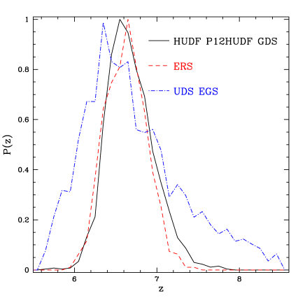
Figure 1: The selection function in redshift for the different color criteria adopted in the six CANDELS and HUDF fields. The peaks of the distributions have been normalized to 1 to ease the comparison. The selection function for the CANDELS wide surveys (UDS and EGS) is more extended due to the limited set of filters used (VIJH) with respect to the filters used in GOODS Deep or HUDF surveys (BVIZYJH).

3.1 The reliability of candidates selected on the CANDELS Wide surveys

In the CANDELS wide surveys analysed here (UDS and EGS), the reliability of $z\sim 7$ galaxies candidates can be hampered by the limited set of HST images (VIJH) available. We have carefully investigated the properties of our dropout candidates in the UDS field using both the photometric redshift technique based on SED fitting and the stacking of HST images of all the candidates to check the expected non detection in the optical images.

To compute the photometric redshifts for our candidates in the UDS field, we complement the VIJH HST photometry with the ground based images available from CFHT in the U band, from Subaru in the BVRiz filters and from UKIRT in the JHK bands. We added also the IRAC photometry both from SpUDS and SEDS programs, using the TFIT software to match the resolution of HST to the PSF of ground based images or of space based images by Spitzer. The adopted technique for the derivation of the photometric catalog is described in detail in Galametz et al. (in prep.).

The photometric redshift analysis used to selected the high-redshift candidates in the UDS field was performed using the template-fitting code developed by McLure et al. (2011). For the purposes of this study we employed the Bruzual & Charlot (2003) stellar evolution models, with metallicities ranging from solar ($Z_{\odot}$) to $1/50$th solar ($0.02Z_{\odot}$). Models with instantaneous bursts of star-formation, constant star-formation and star-formation rates exponentially declining with characteristic timescales in the range 50 Myrs $<\leavevmode\nobreak\ \tau\leavevmode\nobreak\ <$ 10 Gyrs were all considered. The ages of the stellar population models were allowed to range from 10 Myrs to 13.7 Gyrs, but were required to be less than the age of the Universe at each redshift. Dust reddening was described by the Calzetti et al. (2000) attenuation law, and allowed to vary within the range $0.0<A_{V}<2.5$ magnitudes. Inter-galactic medium absorption short-ward of Ly$\alpha$ was described by the Madau (1995) prescription, and a Chabrier IMF was assumed in all cases. For each model of this grid, we have computed the expected magnitudes in our filter set, and found the best–fitting template with a standard $\chi^{2}$ normalisation.

Within the UDS sample, only 27 galaxies have a robust photometric redshift $z\geq 6.8$, while the remaining galaxies are either consistent with having a slightly lower value ($6.3\leq z\leq 6.8$), or have two comparable solutions for the photometric redshifts (one at $z\sim$2 and the other at $z\sim 7$). These 27 candidates are part of another work on the luminosity function of bright z-dropout LBGs and will be described in detail in McLure et al. (in prep.), with a full description of the photometric redshifts used here. We decided to keep the full sample of 46 candidates for UDS in our work, after checking that they have comparable properties (both in luminosity and half light radius) to the sub-sample of the 27 candidates of McLure et al. (in prep.). We repeat the same check on EGS, and we find that 13 galaxies out of 21 have $zphot\geq 6.8$.

Fig.2 shows the weighted mean of the 46 $I_{814}$-dropout candidates in the UDS field for $V_{606}$, $I_{814}$, $J_{125}$, and $H_{160}$ bands. The stack image has no detection in the $V_{606}$ band, and a very faint detection in the $I_{814}$ band. The fit to the SED of the stack indicates that the photometric redshift is consistent with $zphot\sim 6.5-7.5$ and no secondary peak at $z\sim 1-2$ is present. Restricting the sample to galaxies with magnitude $J_{125}\leq 26.2$ and angular size $Rh\geq 0.2$ arcsec, we obtain essentially the same stacked SED and photometric redshift probability as that for the whole sample. This indicates that the 46 candidates in the UDS field are robust against contamination by low-z interlopers, and bright and extended $I_{814}$-dropouts are not dominated by foreground sources mimicking our color criteria. In the other fields, where the depth of HST images are similar (EGS) or deeper (ERS, GDS, HUDF, P12HUDF), we expect as well a reduced contamination by lower-z sources.

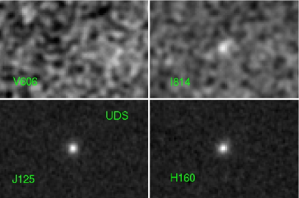
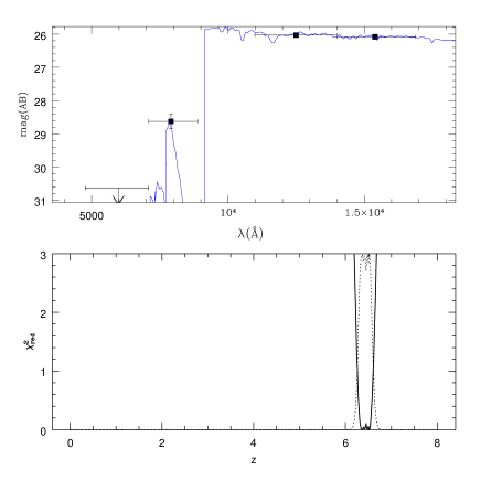
Figure 2: Top: the image stacking of the 46 $I_{814}$-dropout candidates in the UDS field for $V_{606}$, $I_{814}$, $J_{125}$, and $H_{160}$ bands. Middle: the VIJH photometry of this image stacking (black dots) has been fitted with an extended library of synthetic galaxies, and the best fit (blue line) is consistent with a photometric redshift $z\geq 6.5$, with no secondary peak at $z\sim 1-2$. The model templates are computed with the spectral synthesis models BC03 (Bruzual & Charlot (2003)), and chosen to broadly encompass the variety of star–formation histories, metallicities and extinction of real galaxies, as described in detail in McLure et al. (2011). At z=6.5 the Lyman continuum absorption is at an observed wavelength of $\lambda=6840$ Å, and a faint emission in the $I_{814}$ filter can be still compatible with a partially neutral IGM at this redshift. Bottom: The continuous curve is the reduced $\chi^{2}$ as a function of photometric redshift $z$, while the dotted line is the probability P(z) rescaled to have the peak at the same level of $\chi^{2}$, to improve visibility.

4 Simulations for estimating completeness and systematic effects

While the selection criteria described above are formally designed to select a pure sample of high-z candidates, they are in practice applied to very faint objects, typically close to the limiting depth of the images. At these limits, systematics may significantly affect their detection and the accurate estimate of their colors or apparent dimensions. To take into account all the systematic effects (completeness, photometric scatter, size scatter) involved in the size-luminosity relation, we carried out a set of detailed simulations.

These simulations have two main goals. The first is to estimate the incompleteness that affects the detection of faint galaxies as a function of their size. The incompleteness arises not only from the difficulty of detecting faint sources, but also from the effect of noise in the many bands that we need to select high-z candidates. As expected, we become severely dominated by incompleteness as we attempt the detection of extended sources at the faintest magnitudes, and this effect must be taken into account when trying to infer the intrinsic size–luminosity relation.

The second goal is to quantify the systematic biases in the measure of the half–light radius provided by SExtractor, as a function of magnitude and galaxy size. These systematic biases affect the estimate of the distribution of galaxy size in a non-negligible way, and therefore also need to be treated carefully in the analysis.

In this section we describe in some detail the simulations adopted to estimate these systematic effects and the technique that we adopt to include them in the derivation of the correct size distribution. The reader directly interested in the observational results may skip this section and proceed to Sect. 5.

4.1 Completeness

We follow the procedure described in Grazian et al. (2011) and in Castellano et al. (2010a, b) to obtain a realistic catalog of simulated high redshift sources. We first produce a set of UV absolute magnitudes and redshifts $(M_{1500},z)$ according to an evolving Luminosity Function by Castellano et al. (2010b), and then convert it into a set of predicted magnitudes using the BC03 models with a range of ages, metallicities, dust content and Ly$\alpha$ emission as in in Grazian et al. (2011). We have also added the intergalactic (IGM) absorption using the average evolution as in Fan et al. (2006). The redshift range adopted for the simulated galaxies in all the fields is $5.5<z<8.5$ while the absolute magnitudes $M_{1500}$ run from -17 to -23. The input distribution for the axial ratio parameter $b/a$ is assumed flat from 0 to 1.

For each simulated galaxy, an input half-light radius has been assigned by selecting at random from a uniform distribution between 0.0 and 1.0 arcsec. The two-dimensional profiles adopted during the simulations are typical of disk galaxies, i.e. an exponentials. In Appendix B we show the results of our simulations under the assumption of a Sersic profile of index $n=4$. Previous works (e.g. Ferguson et al. (2004)) dealing with the size-luminosity relation at lower-z, assumed a mix of morphological models, with a fraction of 70% spiral and 30% ellipticals at z=3-4. From the observational point of view, Ravindranath et al. (2006) find that 40% of the LBGs at $2.5<z<5$ have light profiles close to exponential, as seen for disk galaxies, and only $\sim$30% have high Sersic index, as seen in nearby spheroids. They also find a significant fraction ($\sim$30%) of galaxies with multiple cores or disturbed morphologies, suggestive of close pairs or on-going galaxy mergers. Using the ultradeep images of the HUDF in BVIZ bands by ACS, Hathi et al. (2008b) found that the sum of the images of all LBGs selected at $4\leq z\leq 6$ are well fit by Sersic profiles with an index $n<2$, indicating that these galaxies follow a disk-like profile in their central region, as recently confirmed by Fathi et al. (2012) (but see Graham & Guzman (2003) for a different interpretation). Moreover, recent results from spectroscopically confirmed LBGs at $z\leq 3$ (Nagy et al. (2011); Law et al. (2012)) and $z\sim 5$ (Douglas et al. (2010)) show that the light profile of these galaxies are not represented by an elliptical morphology, and the brightest galaxies are typically described by an exponential disk. Based on these considerations, from now on we assume that galaxies at $z\sim 7$ are typically approximated by an exponential disk morphology and that there is no galaxy with an $r^{1/4}$ profile at such high-z. Though this is only a rough approximation, there are indications, at redshifts lower than 7, that it is a realistic assumption.

The synthetic galaxies are placed at random positions in the real 2-dimensional FITS images, avoiding positions where where real galaxies or stars are observed. To this aim, the segmentation image created by SExtractor during the detection of real objects in the observed J band has been used for each field. To avoid an excessive and unphysical crowding in the simulated images, we have included only 200 objects of the same flux and morphology each time. We then perform the detection in the synthetic images using SExtractor with the same parameters adopted for the real images. We simulate all the available bands, i.e. from the B to the H bands for the ERS and HUDF fields while for the UDS and EGS fields we have simulated only the VIJH filters from HST observations. We repeated the simulation until a total of at least $5\times 10^{5}$ objects were tested for each of the six fields described above.

These simulations first provide the detection completeness as a function of the input half light radius and input total magnitudes. The typical output is shown in Fig.3, where we plot the measured total magnitude $J_{out}$ and half-light radius $Rh_{out}$ in the case of the UDS field. Small dots show the position of the simulated objects, while big red triangles are the observed $z\sim 7$ LBG candidates. Since the simulated input catalog contains objects of all sizes up to 1” in equal proportions, Fig.3 clearly shows that, at a given magnitude, the fraction of detected objects drops above some critical size. We use these simulations to compute the 50% completeness threshold as a function of magnitude, which is shown as a blue solid line in Fig.3.

We repeated the same analysis for all the six fields in our survey and we show the output in Fig.14 of Appendix B, for the EGS, ERS, GDS, P12HUDF and HUDF fields, respectively. Results are qualitatively very similar, the only major difference being that the 50% completeness curve shifts to fainter magnitudes on the deeper fields, as expected.

We also explored the effects of our assumption for the galaxy surface-brightness profiles. We repeated the analysis adopting as input for our simulations a Sersic profile with index $n=4$, and show the completeness obtained with this profile in Fig.3 (dashed line), comparing it with the previous result for an exponential profile (solid line). As expected, the 50% completeness threshold occurs at lower radii (for a given magnitude) with the elliptical profile than with the exponential one. It is worth noting that the elliptical profile cannot explain the presence of galaxies brighter than $J=26$ and larger than 0.3 arcsec in half light radius that we are finding in the UDS field. It is useful to stress that the completeness due to a Sersic profile with index $n=4$ carried out here is only a simple exercise and in the following sections of this paper we make the reasonable assumption that all the $z\sim 7$ candidates found in the CANDELS and HUDF fields have an exponential disk profile.

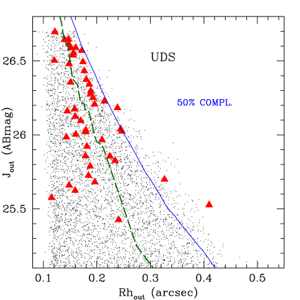
Figure 3: The observed J magnitude vs size of simulated (small black dots) and observed galaxies (red triangles) at $z\sim 7$ for the UDS field. The solid blue line shows the 50% completeness level for an input simulated profile of disk galaxy, while the dashed green line is the same limit for a Sersic profile with n=4.

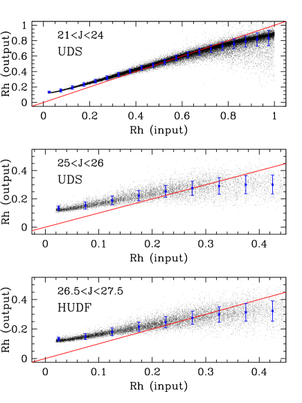
Figure 4: The results of our simulations for $z\sim 7$ galaxies with exponential disk profiles in the UDS and HUDF fields. The plot shows the comparison between the half–light radius (in arcsec) as measured by SExtractor as a function of the input one. The upper and lower panel refer to different total magnitudes in two different simulations, as reported in the legend. The red line shows the identity relation. The blue points and errorbars show the average value and the relevant r.m.s. of the output half–light radius. At small sizes the output half light radius is typically larger than the input one due to the convolution with the instrumental PSF carried out during the simulations. Note that the limits of the top panel are different from the ones in the middle and bottom panels.

A second output of our simulations is the estimate of the biases in the measurement of the half–light radius as a function of luminosity and size. We show the results in Fig.4, where we plot the measured $Rh$ as a function of the input one, in three magnitude ranges. The upper and middle plots refer to the UDS field, while the bottom plot describes the same simulation for the HUDF field. The upper panel shows the result for relatively bright objects ($21\leq J\leq 24$). While no $z\simeq 7$ galaxies are found in this magnitude range, it is instructive to see that systematic effects are important even at the bright end. As expected, the measured size of the objects cannot be smaller than the instrumental PSF (which is about 0.18” of FWHM in the J band, corresponding to an half light radius of 0.11”). Because of the convolution with the PSF, all objects intrinsically smaller than $\simeq 0.2$” are biased high by the SExtractor estimate. Above 0.4”, the opposite starts to occur. This is due to the detection algorithm adopted. In SExtractor an object is detected only if a given number of pixels have an intensity above a defined threshold, and the half light radius is computed using only those pixels. For faint and quite extended galaxies, the surface brightness far from the center is very low and the galaxy merges into the noise, with the effect of underestimating both the total flux and the effective size for these objects. The middle and bottom panels of Fig.4 show the same simulations carried out in two magnitude ranges that are critical for the aims of this work (note that the half light radius range in the x and y-axis is different from the one in the top panel).

The combined effect of the two systematic biases described above (on the detection and on the estimated size) has a measurable impact on the observed distribution of galaxy sizes. An example is given in Fig.5. We assume that the real input distribution is a log-normal with mean half light radius of 0.6 arcsec and a $\sigma_{Rh}$ of 0.5 (black histogram) which has a mode (peak) at 0.2 arcsec. These values are not representative of the best fitting parameters for the UDS half light radius distribution, but they are randomly chosen just to provide an example with an extended tail, to show the selection effects at large $Rh$.

The distribution of the measured sizes (red histogram) of the simulated objects deviates from the input distribution in two respects. At small sizes, the distribution is truncated below 0.1-0.15” and the peak is moved to a slightly larger value, because of the convolution with the PSF. At large sizes, a clear cut above half light radius of 0.4 arcsec is evident, due to the detection incompleteness discussed in Fig.3. We also note that when the color criteria for $z\sim 7$ are applied, the amplitude of the histogram is reduced but its shape is not changed (magenta distribution), implying that the color selection is not significantly affecting the half–light distribution of the simulated objects. The $Rh$ distribution for real objects, scaled in normalization to match the number of simulated galaxies, is shown by the blue histogram in Fig.5.

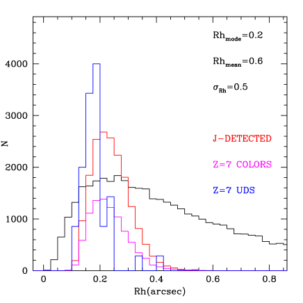
Figure 5: The size distributions of simulated and observed galaxies at $z\sim 7$ for the UDS field. The black histogram represents the input log-normal function with mean half light radius of 0.6 arcsec and a $\sigma_{Rh}$ of 0.5, resulting in a peak at 0.2 arcsec (mode). This is not the best fit for the observed size distribution, but only an example to show the effects of incompleteness at large half light radii. The input galaxies are simulated down to a magnitude of $J=26.7$, which is the nominal limit for the UDS field. The red histogram is the size distribution of all galaxies detected in the J band UDS image, irrespectively of magnitudes and colors, while the magenta histogram shows only the galaxies at $z\sim 7$ selected by our color criteria. Last, the blue distribution represents the observed galaxy sizes in the UDS, scaled in normalization to match the number of simulated galaxies.

4.2 Finding the best fit to the observed distribution of galaxy half–light radius

We finally use our simulations to recover the true size distribution of z=7 galaxies, under the assumption of a particular functional form. We parameterized this as a log-normal function in half light radius, with the two parameters $Rh_{mode}$ and $\sigma_{Rh}$ that are independent from the input luminosities for each simulated sample. This assumption is based on the fact that the observed size distribution at different redshifts is characterized by a well-defined peak and a tail towards more extended objects (e.g. Nagy et al. (2011)). The log-normal functional form naturally fits this shape, and it is characterized by two parameters, $Rh_{mode}$ and $\sigma_{Rh}$, the peak and the dispersion of the log-normal half light radius distribution. Moreover, from the theoretical point of view, the log-normal function is expected as a natural distribution for galaxy sizes (Mo, Mao & White (1998)).

In order to recover the intrinsic shape of the distribution we have adopted a Maximum Likelihood (ML) approach. For any choice of the free parameters of the log-normal function ($Rh_{mode}$ and $\sigma_{Rh}$), the resulting intrinsic distribution is first convolved with the observational biases (as described above, see Fig.5) to get the expected number of sources as a function of the measured half light radius. The total number of observed galaxies has been matched to the simulated one. Then, a Poisson likelihood is computed comparing the simulated and observed $Rh$ distributions, using the usual formula:

$${\cal L}=\prod_{i}e^{-N_{exp,i}}\frac{(N_{exp,i})^{N_{obs,i}}}{(N_{obs,i})!}$$ (1)

where $N_{obs,i}$ is the observed number of sources in the half light radius interval $i$, $N_{exp,i}$ is the expected number of simulated sources in the same half light radius interval, and $\Pi_{i}$ is the product symbol.

Because the observed J-band magnitude range of our $z\sim 7$ candidates in the six CANDELS fields is roughly two magnitudes, and even larger for HUDF and P12HUDF, we limit both the observed and the simulated samples to a relatively small magnitude interval for the maximum likelihood computation. For each field, we use only galaxies (both observed and simulated) in the magnitude range $25.6\leq J\leq 26.6$ to compute the likelihood for bright galaxies; for the intermediate magnitude bin we limit the interval to $26.6\leq J\leq 27.6$, while for the faintest bin we adopt $27.6\leq J\leq 28.6$ as limits. Even though a size-luminosity relation holds at $z\sim 7$, as we will show later in this paper, this choice ensures that the change in $Rh_{mode}$ inside each analysed magnitude interval is small.

For each combination of the two parameters $Rh_{mode}$ and $\sigma_{Rh}$, the peak and the dispersion of the log-normal half light radius distribution, we compute the maximum likelihood as described in Eq.1. A typical example is provided in Fig.6, that shows the best fit distribution resulting from comparing observations and simulations in the UDS field, using $z\sim 7$ galaxies in the magnitude range $25.6\leq J\leq 26.6$. We plot both the differential (bottom) as well as the cumulative size distributions (top). This figure shows the observed distributions of half light radii (black segmented line) and a comparison is made with the cumulative distributions resulting from the simulations discussed above (blue curve) after all the systematic effects are taken into account, especially the convolution of the intrinsic galaxy shape with the observed PSF. We compute the Kolmogorov-Smirnov p-value by comparing the observed and the simulated cumulatives. Since the K-S test is not sensitive to the details of the distribution, we prefer the Maximum Likelihood approach (bottom panel), as we discussed above, to find the best agreement between simulations and observations.

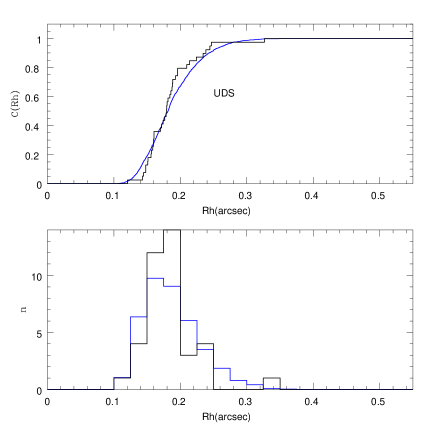
Figure 6: The best fit for the size distribution of the observed galaxies at $z\sim 7$ in the magnitude range $25.6\leq J\leq 26.6$ for the UDS field. Top: the cumulative distribution for the observed galaxy sizes (black histogram) is compared with the same for the simulated galaxies (blue curve), and a K-S p-value is computed. Bottom: The observed (black) and simulated histograms (blue), as described in the top panel, are compared with a Maximum Likelihood approach.

For each of the six fields we scan a grid in two parameters, $Rh_{mode}$ and $\sigma_{Rh}$. The grid extends from 0.01 to 0.4 arcsec in $Rh_{mode}$ (corresponding to an interval of 0.02-1.0 arcsec in $Rh_{mean}$) and from 0.02 to 1.0 arcsec in $\sigma_{Rh}$, for a bin size of 0.01 arcsec in $Rh_{mode}$ and 0.02 in $\sigma_{Rh}$. The choice of parameters ($Rh_{mode}$, $\sigma_{Rh}$) that maximizes the likelihood is considered as the best fit for the real input distribution. To improve the signal-to-noise ratio of the fitting procedure, we combine the likelihoods of the fields within the same J-band magnitude range. In addition to the best fit values, the ML approach allows us to define the allowed confidence intervals on the free parameters $Rh_{mode}$ and $\sigma_{Rh}$.

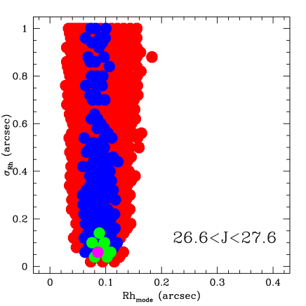
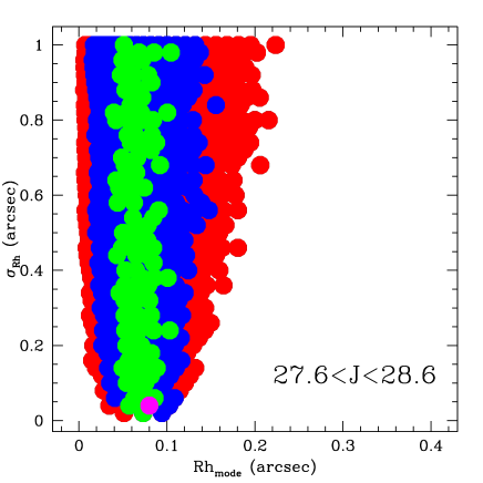
Figure 15: The composite likelihood distribution for the intermediate ($26.6\leq J\leq 27.6$, left) and faint ($27.6\leq J\leq 28.6$, right) magnitude bins. The best fit is indicated by the magenta point while the green, blue, and red regions define the uncertainties at 68%, 95%, and 99.7% (1,2, and 3 sigma) confidence level, respectively.

Fig.7 shows the likelihood distribution for the combined UDS, EGS, ERS and GDS fields for galaxies in the magnitude range $25.6\leq J\leq 26.6$. The best fit is indicated by the magenta point while the green, blue, and red regions define the uncertainties at 68%, 95%, and 99.7% (1,2, and 3 sigma) confidence level, respectively. In Fig.7 $Rh_{mode}$ and $\sigma_{Rh}$ represent the intrinsic parameters of the input log-normal distribution before convolving it with all the observational effects (PSF convolution, noise, detection and size measurements). Fig.15 in Appendix C shows the same plot for the other J band intervals, namely the combination of all the fields for the intermediate magnitude bin $26.6\leq J\leq 27.6$, and the combined GDS, P12HUDF and HUDF fields for the faintest bin $27.6\leq J\leq 28.6$, respectively. From this statistical analysis we derive the best fit values $Rh_{mode}$ and $\sigma_{Rh}$ used in the following, together with their 68% confidence level intervals.

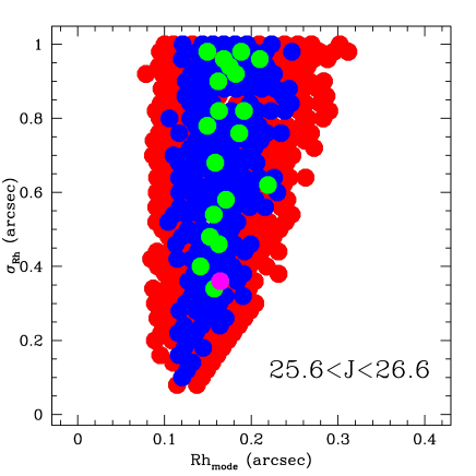
Figure 7: The confidence levels obtained with the maximum likelihood approach for the size distribution on the magnitude interval $25.6\leq J\leq 26.6$. The best fit is indicated by the magenta point while the green, blue, and red regions define the uncertainties at 68%, 95%, and 99.7% (1,2, and 3 sigma) confidence level, respectively. The $\sigma_{Rh}$ is basically unconstrained, while the parameter $Rh_{mode}$ is well constrained between 0.14 and 0.22 arcsec at 1 sigma.

In Fig.7 the peak of the half light distribution ($Rh_{mode}$) for the bright sample ($25.6\leq J\leq 26.6$) is well constrained by the present observations, while it is not possible to put reasonable limits for the spread of the size distribution ($\sigma_{Rh}$). The reason for this behavior is clear going back to Fig.5: input distributions with extended tails like the black histogram, after the convolution with simulated effects, are affected by a strong incompleteness at large sizes (red and magenta histograms) and thus the present data in the UDS and EGS fields, even after detailed comparison with simulations, cannot provide stringent constraints to the extensions of the intrinsic distributions in size.

5 Results

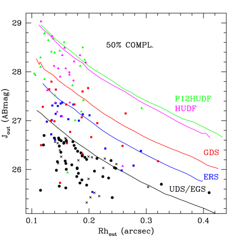
Figure 8: The observed J magnitude vs size of candidate galaxies at $z\sim 7$ for all the six fields analysed. The black circles indicates galaxies in the UDS field, while crosses are associated to objects in the EGS field. The solid lines show the 50% completeness levels of the six different surveys for an input simulated profile of exponential disk galaxy. The galaxy size ($Rh_{out}$) is the observed half light radius in arcsec measured by SExtractor and it is not deconvolved by the PSF.

5.1 Faint galaxies are always small

First of all, we present the relation between galaxy half light radii and fluxes for our $z\sim 7$ sample. Fig.8 summarizes the result for the observed size-magnitude distribution at $z\sim 7$ for all the six fields investigated in this work. The solid lines show the 50% completeness levels of the six different surveys for an input simulated profile of exponential disk galaxy, as described above. The galaxy size ($Rh_{out}$) is the observed half light radius in arcsec measured by SExtractor, without any attempt to deconvolve it for the effect of the PSF.

It is interesting to note in this plot the lack of galaxies in the region of large sizes but faint magnitudes (or low surface brightness) objects, namely fainter than J=26.6 and larger than 0.2 arcsec (corresponding to a physical dimension of 1.15 kpc at z=7). Two notable exceptions are 2 galaxy candidates, one in the GDS and the other in the P12HUDF field. Visual inspection of these two objects indicates that they are both close to bright and extended galaxies, thus their magnitudes or sizes could be affected by the presence of the bright interlopers. They do not show any evidence of merging or clumpy morphology. We included these two galaxies in the Maximum Likelihood analysis described above. Excluding these two objects from Fig.8, we detect a clear lack of faint and extended galaxies at $z\sim 7$, corroborated by very large statistics (153 candidates over 6 fields) and down to very faint magnitude limits ($J\sim 29$). Limiting our analysis to $26.6<J<27.6$, where the lack of extended galaxies is evident and where we are reasonably complete with our survey, we have 41 galaxies. Moreover, as shown in Fig.4 (bottom panel), in this magnitude range the true value of the galaxy size is not particular underestimated, and from our simulations we expect to find exponential disk galaxies with $Rh=0.3-0.4$ arcsec, if they exist. None of them have been found on HUDF and P12HUDF.

From the best fit results of Fig.7 and Fig.15 in Appendix C it is clear that the parameter $\sigma_{Rh}$, which regulates the amplitude of the log-normal distribution in size, is basically unconstrained in almost all the fields (see also Table 1). It is also worth noting that in Fig.15 we have a marginal indication (68% confidence level) that the parameter $\sigma_{Rh}$ is less than 0.14 arcsec on the magnitude interval $26.6\leq J\leq 27.6$. If confirmed, this could strengthen the evidence of a lack of extended galaxies at z=7 in the faint luminosity regime ($J\sim 27-28$). Conversely, as shown in Fig.8, at magnitude brighter than $J=26.6$ (i.e. $M_{1500}\sim-20.5$ for z=7) galaxies can be as extended as $Rh=0.4$ arcsec, or 2.3 kpc physical, while fainter than this limit the sizes are always less than 0.2 arcsec.

5.2 The best fit log-normal distribution

The visual impression derived from Fig.8 is confirmed by the robust analysis with the ML method. Adopting the formalism described above, we fit the observed size distributions in the six fields with a log–normal function, taking into account all the observational biases. Results are summarised in Fig.9, where we plot the peak (mode) half light radius (of the intrinsic distribution) at different luminosities of the $z\sim 7$ galaxy candidates in each survey. The brightest point refers to galaxies in the magnitude range $25.6\leq J\leq 26.6$, while the middle point at $M_{UV}\sim-19.5$ is the result of the joint Maximum Likelihood using objects with $26.6\leq J\leq 27.6$. In the faint bin we combine the Likelihood values for the GDS, HUDF, and P12HUDF fields at $27.6\leq J\leq 28.6$. The vertical error bars are the 1$\sigma$ uncertainties on $Rh_{mode}$ found with the simulations described above, while the horizontal error bars show the minimum-maximum range in luminosity of the sample. The results for each magnitude interval are summarized in Table 1.

Table 1: Size-Luminosity Results at $z\sim 7$

Interval	$N_{cand}$	$M_{UV}$	$M_{UV}^{min}$	$M_{UV}^{max}$	$Rh_{mode}$	$Rh_{mode}^{low}$	$Rh_{mode}^{up}$	$\sigma_{Rh}$	$\sigma_{Rh}^{low}$	$\sigma_{Rh}^{up}$
					(arcsec)	$-1\sigma$	$+1\sigma$	(arcsec)	$-1\sigma$	$+1\sigma$
$25.6\leq J\leq 26.6$	63	-20.5	-21.0	-20.0	0.16	0.14	0.22	0.36	0.34	0.98
$26.6\leq J\leq 27.6$	36	-19.5	-20.0	-19.0	0.09	0.07	0.11	0.06	0.04	0.14
$27.6\leq J\leq 28.6$	32	-18.5	-19.0	-18.0	0.08	0.04	0.10	0.04	0.02	1.00
$26.6\leq J\leq 28.6$	68	-19.0	-20.0	-18.0	0.09	0.08	0.10	0.06	0.04	0.10

$N_{cand}$ is the number of galaxy candidates at $z\sim 7$ used in this work, with observed magnitudes $25.6\leq J\leq 26.6$, $26.6\leq J\leq 27.6$, and $27.6\leq J\leq 28.6$ in the six fields analysed here. The columns $M_{UV}^{min}$ and $M_{UV}^{max}$ refer to the minimum and maximum in absolute magnitudes of the observed sample, while $Rh_{mode}^{low}$ and $Rh_{mode}^{up}$ indicate the 1$\sigma$ lower and upper limits for the $Rh_{mode}$ parameters, in arcsec. The last two columns indicate the 1$\sigma$ uncertainties for the parameter $\sigma_{Rh}$, in arcsec.

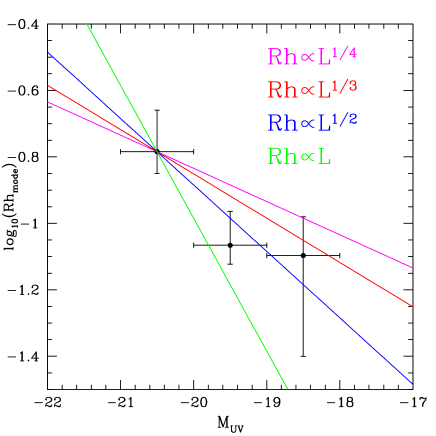
Figure 9: The trend of galaxy size (in arcsec and logarithmic scale) with UV absolute magnitude (1500Årest frame) at z=7 and the comparison with some simple power-law relations. The data point at $M_{UV}\sim-20.5$ is related to galaxies in the magnitude range $25.6\leq J\leq 26.6$, the one at -19.5 is derived using objects with $26.6\leq J\leq 27.6$, while the faint bin at -18.5 is the combination of GDS, HUDF, and P12HUDF fields (where the maximum likelihood has been computed restricting to $27.6\leq J\leq 28.6$).

Overplotting simple power-law relations in Fig.9, it is clear that there is a strong dependence of the size on luminosity, $Rh\propto L^{1/2}$ or $Rh\propto L^{1/3}$. We cannot exclude however that the size distribution is a constant function ($Rh\sim 0.16$ arcsec) at $L>L^{*}$ and then there is a cutoff to 0.08 arcsec (=0.4 kpc at z=7) for fainter galaxies, rather than being represented by a smoother trend with luminosity. The point at $M_{UV}=-18.5$ deserves also particular attention: it is the combination of two fields in particular, the HUDF and P12HUDF, since the five GDS galaxies at $J\sim 27.6$ are not able to provide strong constraints to the size distribution. If we check the results of the two ultradeep fields separately, we find two different best fit values, $Rh_{mode}=0.09\pm 0.02$ arcsec for HUDF and $Rh_{mode}=0.03\pm 0.03$ for P12HUDF. The differences between these two samples are also evident in Fig.8, where the typical galaxies in the HUDF have a larger observed $Rh$ with respect to the ones in the parallel field. The two inconsistent results can be due to the small volumes covered by these two HST pointed observations, which can be affected by a strong field to field variation. Larger areas covered by HST at a similar depth of the HUDF are thus required in order to solve the inconsistency of $Rh$ estimate at faint magnitude limits.

The faint bin of the size-luminosity relation in Fig.9 is particularly problematic also for another reason. From Fig.4 it is clear that in the HUDF and P12HUDF, for galaxies with input $Rh<0.1$, the size of galaxies as measured by SExtractor is completely dominated by the PSF of HST and the resulting $Rh(output)$ is around 0.12 arcsec. This feature in the HUDF and P12HUDF fields is present both for relatively bright ($J\sim 26.5$) and for faint ($J\sim 28.5$) simulated galaxies. Moreover, at $J\sim 28-28.5$, the galaxy size is under-estimated for simulated objects with input $Rh$ greater than 0.2 arcsec. Thus, it is reasonable to think that the present $z\sim 7$ galaxies at $J\sim 28$ cannot give strong constraint to $Rh_{mode}$ estimation, and the behavior of the size-luminosity relation for $M_{UV}\geq-19$ is presently not robust.

To check the reliability of the $Rh_{mode}$ determination at the faintest magnitudes, we have also investigated in the HUDF the power of the maximum likelihood test on the discrimination between different best fit solutions. The relatively large PSF of WFC3 with respect to the expected size of galaxies at z=7 and $M_{UV}>-19$ can induce the reader to think that it is not possible to distinguish between values of $Rh_{mode}$ smaller that $\sim 0.1$ arcsec at $J\sim 28$. We have verified for HUDF galaxies in the magnitude range $27.6<J<28.6$ that an input distribution with $Rh_{mode}=0.02$ arcsec has a likelihood parameter that is 3$\sigma$ off from the best fit ($Rh_{mode}=0.08$ arcsec), while if we choose $Rh_{mode}=0.14$ arcsec the likelihood test can reject this solution at 2$\sigma$ level. Thus, we can conclude that our simulations are able to distinguish between values of $Rh_{mode}$ smaller than the actual size of the WFC3 PSF. As we discussed above, the main uncertainty on the size determination at $M_{UV}>-19$ is the field-to-field variance, with significantly different values between the HUDF ($Rh_{mode}=0.09\pm 0.02$ arcsec) and the P12HUDF field ($Rh_{mode}=0.03\pm 0.03$ arcsec).

From these results we can draw another conclusion. While we could not exclude the presence of a non negligible population of faint and extended galaxies, it is clear that the typical (mode) physical dimension at $L\leq L^{*}$ is smaller than for more luminous galaxies. A similar result has been found on the HUDF also by Oesch et al. (2010b).

We thus have found evidence for a size-luminosity relation (in the sense that bright galaxies can be extended while faint galaxies are always compact/small) at high redshifts, confirming the general trend found by star forming galaxies (LBGs, LAEs) at lower-z (Nagy et al. (2011); Bond et al. (2012); Law et al. (2012)). This is also in agreement with the works of Vanzella et al. (2009); Pentericci et al. (2010); Malhotra et al. (2012): they found that LAEs at $z\sim 3-4$ are in general smaller than the LBG sample and fainter in the UV continuum. They also showed that galaxies with small or negative EW in Lyman-$\alpha$ span a wide range of sizes and UV continuum luminosities, while large EW objects tend to be very small and faint in $M_{UV}$, in practice line emitters tend to be small galaxies, while amongst LBGs there are both small and large galaxies.

A comparison can be carried out at this stage between the size/luminosity relation of LBGs at $z\sim 7$ with the one of star-forming galaxies at lower-z. Papovich et al. (2005) found that the typical size of spiral galaxies with $M_{UV}\sim-21$ at $z\sim 2-3$ is $\sim 2kpc$, slightly larger than our determination ($\sim 0.8$ kpc) at the same luminosity. We can thus infer that the size-luminosity relation of star-forming galaxies is evolving slowly from $z=7$ to $z=2$, in agreement with the $(1+z)^{-1}$ evolution of $Rh$ with redshift found by Bouwens et al. (2004) at lower-z and confirmed by Hathi et al. (2008) at $z\sim 5-6$ and by Oesch et al. (2010b) at $z\sim 7$.

Local irregulars and spirals are characterized by a similar size-luminosity relation. Roche et al. (1996) derived a relation between the half light radius and the luminosity at $z\sim 0.5$ of $Rh\propto L^{1/2}$. Fig.10 summarizes the size-luminosity relations at various redshifts described above, showing a continuous evolution in $Rh$ from z=7 (our points) to z=1-3 (the empty squares and triangles by Papovich et al. (2005)). At lower redshift the situation is currently not clear, with Roche et al. (1996) finding a steep relation between the half light radius and the luminosity of galaxies at z=0.5, $Rh\propto L^{1/2}$, while de Jong & Lacey (2000) measured a flatter relation $Rh\propto L^{1/3}$, and slightly lower in normalization at $M_{UV}=-21$ for the local galaxies. Despite this discrepancy at lower-z, the normalization of the local size-luminosity relation is higher at low-z than at $z\sim 2-7$: a spiral/irregular galaxy with $M_{UV}\sim-21$ has a physical (proper) size of 6-10 kpc at $z<1$, compared to 2 kpc at $z\sim 2$. This implies that a significant evolution on the size/luminosity relation happened in the last 8 Gyr of the lifetime of the Universe, in contrast with a slow growth at $z\geq 2$.

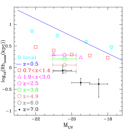
Figure 10: The redshift evolution of the size-luminosity relation from $z\sim 0$ to z=7. The cyan empty stars show the local relation found by de Jong & Lacey (2000), taking the absolute magnitudes in the I band from their work and applying a constant shift $M_{UV}-M_{I}=1.0$. The blue line is the relation by Roche et al. (1996) for irregular galaxies at $z\sim 0.5$, the empty squares and triangles represent galaxies at $0.7<z<1.4$ and $1.9<z<3.0$ by Papovich et al. (2005) and the pentagons are the typical half light radii of LBGs at z=2.5 (magenta, top), 3.8 (green), 4.9 (brown), and 6.0 (grey, bottom) by Bouwens et al. (2004). The black dots with error bars are the z=7 relation found in this work.

6 Discussion

6.1 The impact on the reionization process

The presence of a size/luminosity relation at $z\sim 7$ has important implications for the luminosity function of LBGs at $z\sim 7$ and the role of stars on the reionization of the Universe. The observed lack of extended galaxies at faint magnitude limits ($Rh\sim 0.2$ arcsec at $J>27$) implies that the typical half light radius is less than $\sim$0.1 arcsec ($Rh_{mode}$).

The present data on individual fields are not able to give stringent constraints on the amplitude of the size distribution ($\sigma_{Rh}$), as described above. We explore here the possibility to sum up the likelihood regions for all the fields probing the faint side of the magnitude distribution, namely the ERS, GDS, P12HUDF and HUDF, in the magnitude range $26.6\leq J\leq 28.6$. Adding together the outputs of these four fields, we derive a best fit of $Rh_{mode}=0.09\pm 0.01$ arcsec and a $\sigma_{Rh}=0.06\pm 0.04$. We thus explore the dependence of the slope of the faint end of the $z\sim 7$ LBG Luminosity Function $\alpha$ on the shape of the half-light radius distribution. We fix the parameters $Rh_{mode}$ to 0.09 and $\sigma_{Rh}$ to 0.06, which are the best fit values found above for the combination of all the faint fields. We compute the number density of $z\sim 7$ LBGs using the stepwise technique as in Grazian et al. (2011) for the HUDF and P12HUDF fields separately and plot the results in Fig.11. At faint absolute magnitudes, $M_{UV}\sim-18$, the field to field variation in the number counts is comparable with the statistical errors (a combination of Poisson noise and uncertainties due to the conversion of observed J band magnitudes into absolute values taking into account the output of our simulations). In particular, in the P12HUDF field an excess of faint $z\sim 7$ galaxies have been detected, which results in a relatively steep LF for this field. We have checked that this enhancement is not due to an artificial overcorrection due to an excess of false positive rejection rate at faint magnitudes in the P12HUDF field. The number of simulated galaxies at $z\sim 7$ which are not recovered by our criteria in this field is 11% and it is similar to that found in HUDF (12%).

We have fitted with a Schechter function (Schechter (1976)) the individual stepwise results for HUDF and P12HUDF adding the LF determinations at $M_{UV}\leq-20.5$ discussed in Grazian et al. (2011) and shown in Fig.11 with filled symbols. Fixing $\Phi^{*}$ and $M^{*}$ to the values provided in Grazian et al. (2011), namely 0.00074 and -20.14, we obtained $\alpha=-1.65\pm 0.09$ and -1.83$\pm$0.18 for the HUDF and P12HUDF, respectively. We can derive a mean value for $\alpha$ by averaging the number counts in the HUDF and P12HUDF fields. We thus obtained $\alpha=-1.7\pm 0.1$, where the large uncertainties reflects the strong field to field variation affecting the present data.

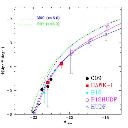
Figure 11: The Luminosity Function of LBG galaxies at $z\sim 7$ computed with the Stepwise method and assuming a log-normal size distribution with parameters $Rh_{mode}=0.09\pm 0.01$ arcsec and $\sigma_{Rh}=0.06\pm 0.04$. The filled symbols show the data points presented in Grazian et al. (2011) (black dots and upper limits by Ouchi et al. (2009); red squares by Castellano et al. (2010b) and cyan dots by Bouwens et al. 2010b ), while the open points are the number densities for the HUDF (triangles) and P12HUDF (circles). The cosmic variance between the two fields is greater than the statistical uncertainties.

If we consider $Rh_{mode}=0.09$ arcsec and $\sigma_{Rh}=0.48$, we obtain the most extended size distribution still allowed at the 95% confidence level by the combined likelihood regions in the magnitude range $26.6\leq J\leq 28.6$. Using this distribution into the simulations, we derived two luminosity functions at $z\sim 7$ for the HUDF and P12HUDF fields as described above, and fitting them with a Schechter function we obtained $\alpha=-1.87\pm 0.12$ and $\alpha=-2.05\pm 0.23$, respectively. Combining the two fields, a best fit of $\alpha=-1.95\pm 0.15$ has been derived. We thus confirm the anti-correlation between the parameter $\sigma_{Rh}$ and the resulting steepness $\alpha$ of the LF, already found in Grazian et al. (2011). In our previous paper, we found that the faint end of the $z\sim 7$ LBG Luminosity Function $\alpha$ is $\sim$-1.7 (see their Fig.8), when a compact morphology ($Rh\leq 0.15$ arcsec) is adopted. For more extended morphologies ($Rh\sim 0.25$ arcsec) a steeper LF was derived ($\alpha\sim-2$), confirming these results.

A plausible value for the relevant UV emissivity of LBGs at $z=7$, $\rho_{UV}$, can be computed by integrating the present z=7 LF with $\alpha=-1.7$ down to $M_{1500}=-10$, assuming that the steepness of the faint end of the LF remains constant down to fluxes significantly fainter than that reached by our deepest images, the HUDF and P12HUDF ones.

Using $M^{*}=-20.14$, $Log\Phi^{*}=-3.13$ for z=7 as in Grazian et al. (2011), we obtain a luminosity density of $\rho_{UV}(-10)=1.1\cdot 10^{+26}$ $erg\leavevmode\nobreak\ s^{-1}\leavevmode\nobreak\ Hz^{-1}\leavevmode\nobreak\ Mpc^{-3}$ corresponding to $\alpha=-1.7$ (the 1 $\sigma$ lower and upper bounds for this quantity are $8.1\cdot 10^{+25}$ and $1.5\cdot 10^{+26}$ $erg\leavevmode\nobreak\ s^{-1}\leavevmode\nobreak\ Hz^{-1}\leavevmode\nobreak\ Mpc^{-3}$, corresponding to $\alpha=-1.6$ and $\alpha=-1.8$, respectively). We have no information on the number density of $z\sim 7$ galaxies at these faint magnitudes ($M_{UV}=-10$) with the present data, so it is useful to stress that this is a very strong extrapolation.

Given these confidence limits on $\rho_{UV}$ and adopting the same assumptions of Grazian et al. (2011), in order to have the Universe ionized at $z=7$ we derive a lower limit for the Lyman Continuum escape fraction $f_{esc}\geq 0.14\times C_{HII}$ for $\alpha=-1.7$, where $C_{HII}$ is the clumpiness of the IGM at z=7. Taking into account the uncertainties on the faint end of the LF, this translates into $f_{esc}\geq 0.10\times C_{HII}$ for $\alpha=-1.8$ and $f_{esc}\geq 0.19\times C_{HII}$ for $\alpha=-1.6$ (at 68% c.l.), respectively.

In the following, we will consider the implications of a luminosity function at z=7 with $\alpha=-1.8$, in order to relax the constraints on the other two parameters, $f_{esc}$ and $C_{HII}$. Assuming a maximum escape fraction of 1.0, the above limits can be converted into constraints to the IGM at z=7, $C_{HII}\leq 10.0$, provided that the only source of UV photons are stars and the Universe is fully ionized at z=7. Of course, smaller values for the clumpiness $C_{HII}$ are required if the escape fraction is less than 100% or the LF is flatter than $\alpha=-1.8$. We must consider $C_{HII}\geq 1$, since galaxies at $z\sim 7$ are formed in biased density regions of the Universe and the IGM is not homogeneous ($C_{HII}=1$) at these redshifts. Limiting the clumpiness to $C_{HII}\geq 1$, we thus have $f_{esc}\geq 0.10$ in order to have the Universe reionized by z=7. Bolton & Haehnelt (2007) have inferred $C_{HII}\leq 3$ at $z\sim 6$ from the Lyman-$\alpha$ forest photoionization state: since $C_{HII}$ is expected to monotonically decrease towards high-z in a hierarchical Universe, an escape fraction of $f_{esc}\sim 0.3$ is enough for stellar ionizers to reach the reionization of the IGM at z=7. A similar result has been derived by Shull et al. (2012), based on hydrodynamical and N-body simulations, of $C_{HII}\sim 1.5-3.0$ at $z\geq 6$. Their model has more free parameters (the electron temperature of the IGM, the IMF of the stellar population producing UV photons) than considered here, and they derived that an escape fraction of 20% is enough at z=7 to keep the Universe ionized.

It is worth noting that the recent estimates of $f_{esc}$ for $L\geq L^{\ast}$ LBGs at $0\leq z\leq 3$ are $\leq 10\%$ (Bridge et al. (2010); Cowie et al. (2010); Siana et al. (2010); Vanzella et al. (2010); Boutsia et al. (2011)): thus, assuming that the Universe is only re-ionized at $z\sim 7$ by stars in galaxies, this implies a fast increase of the galaxy escape fraction going to faint luminosities or to high redshifts (but see Nestor et al. (2011) for a larger estimate of the escape fraction of $L^{\ast}$ LBGs at $z\sim 3$).

We neglect in our computation the contribution of AGNs, since their LF at z=7 is still unknown and the upper limits currently available indicate that the AGN will add only 5-8% to the luminosity density of galaxies (Ouchi et al. (2009); Cowie et al. (2010); Haardt & Madau (2011)). These estimates however are derived extrapolating the behavior of very bright QSOs selected by SDSS ($M_{UV}\sim-26$) down to very faint magnitude limits. Recent results using the 4 Msec Chandra observation in the GOODS-South region pointed out that the X-ray selected AGNs present a rather steep LF toward faint magnitudes (Fiore et al. (2011)), they are characterized by a significant escape fraction (half of them have $f_{esc}\sim$100%, see Vanzella et al. (2010)) and thus they could be the main responsibles of the reionization process at $z\geq 6$.

Summarizing, we have found here that the number density of faint LBGs at $z\sim 7$ can be fitted with a Schechter luminosity function with a faint end slope of $\alpha=-1.7\pm 0.1$, assuming a size distribution with $Rh_{mode}=0.09\pm 0.01$ arcsec and $\sigma_{Rh}=0.06\pm 0.04$. The value of the parameter $\alpha$ depends critically on the size distribution of faint LBGs, as we already found in Grazian et al. (2011), and the slope of the LF at z=7 can be steeper if the half-light radii of LBGs at this redshift extend towards larger values. We have detected the large field-to-field variation in the number density of faint galaxies at $z\sim 7$, but this does not prevent us from deriving a limit on the steepness of the z-dropout LF, $\alpha=-1.7\pm 0.1$ at 68% confidence level. Using this limit, the Universe can be reionized by galaxies at large redshifts, only if their escape fraction is larger than $\sim 30\%$.

A plausible conclusion is that the number of faint galaxies at $z\sim 7$ in the Universe is enough to re-ionize the Universe ($\alpha\sim-1.7$) only when extrapolating the present LF down to $M_{1500}=-10$, assuming a combination of small clumpiness for the IGM and relatively high escape fraction of Lyman continuum photons ($f_{esc}\geq 0.14\times C_{HII}$). A similar conclusion has been reached also by Finkelstein et al. (2012). Since all these conditions are extreme assumptions, we start posing some doubts that the galaxies alone at $z\sim 7$ are able to keep the Universe ionized without the additional contributions of faint AGNs (Fiore et al. (2011)) or other more exotic explanations (Dopita et al. (2011); Conroy & Kratter (2012)). Of course, invoking a dramatic increase of the escape fraction with redshift $f_{esc}\propto(1+z)^{3.4}$ as done in Haardt & Madau (2011) could be an alternative solution to alleviate this problem.

6.2 Is this picture conclusive ?

The picture of the size-luminosity relation sketched in this work might not be conclusive, for a number of reasons: our results are based on photometrically selected candidates and they could be contaminated by lower-z interlopers; the bright side of the distribution is based only on a single field (UDS) and only half of the EGS region, and it is probably affected by the cosmic variance effect, which should be stronger for more luminous galaxies; the morphology adopted in this work (disk galaxies with exponential profile) cannot be representative of the real galaxy shapes, especially at $z\sim 7$ in the UV rest-frame, where the star-forming galaxies are clumpy and irregular; the distribution for the axial ratio parameter $b/a$ assumed in this work (flat from 0 to 1) may not be representative of the real one (see Ferguson et al. (2004));

While we acknowledge that our analysis is not decisive, we tend to believe that these results are robust for a number of reasons.

All the six fields used in this work are characterized by a combination of deep multi-wavelength photometry, which ensures a clean sample of candidate galaxies at $z\sim 7$. The spectroscopic confirmations of the bright candidates in the GOODS fields, and in other ground based surveys, is currently ongoing (Fontana et al. (2010); Stark et al. (2011); Vanzella et al. (2011); Ono et al. (2012)) and the fraction of lower-z interlopers seems to be less than 20% at $z\sim 6$ (Pentericci et al. (2011)). Thus we are confident that the sample adopted for studying the size-luminosity relation in this paper is not heavily contaminated by lower-z galaxies.

At the moment, the bright side of the $z\sim 7$ galaxy population is sampled mainly by the UDS field, so the robustness of the size-luminosity relation is based only on this region. Since the cosmic variance effect should be stronger for more luminous galaxies, one can suspect that it is only by chance that bright galaxies in the UDS are also the largest, when compared to the ones in deeper fields (i.e. HUDF). However, at $J\leq 25.8$ we have 7 galaxies with $Rh\geq 0.2arcsec$ out of a total of 14 objects (50%) in the combined UDS and EGS fields, which is hard to be interpreted only as a simple cosmic variance effect. In the near future the CANDELS-Wide survey will complete the EGS and cover the COSMOS field at a similar depth and areal coverage of the UDS, thus enhancing by a factor of two the number of galaxies in the bright side of the size-luminosity relation and reducing the uncertainties on $Rh_{mode}$.

The size-luminosity relation measured in this work could also be an artifact due to the frequent merging of galaxies expected at very high-z. Instead of measuring a physical size, the large $Rh$ found for relatively bright objects could be an estimate for the separation of their clumps during the merging phase. Detailed kinematic analysis with IFU spectroscopy at Extremely Large Telescopes (ELTs) of 30-40 meters of diameter, as done currently with 8m class telescopes on $z\sim 2$ galaxies (Forster-Schreiber et al. (2006); Law et al. (2012)), would distinguish these two plausible hypotheses.

A more reliable distribution for the axial ratio parameter $b/a$, following Ferguson et al. (2004) can be adopted in our simulations, but we must stress that, in their work, this functional form is measured on a sample of photometrically selected candidate galaxies at $z\sim 4$, and it is not clear whether this should be applied also to our $z\sim 7$ sample. A more detailed approach, like that adopted in Law et al. (2012) work, is more appropriate but very complex and goes beyond the aims of this paper.

7 Conclusions

Galaxy sizes (half light radii) have been measured for a sample of 153 galaxy candidates at $z\sim 7$ from the CANDELS HST Multi-Cycle Treasury Program (Grogin et al. (2011); Koekemoer et al. (2011)) and HUDF09 project (Bouwens et al. (2011)). In particular, we have used the deep HST imaging database in BVIZYJH bands for the ERS, GDS, P12HUDF and HUDF fields together with the wide area observations in the UDS and EGS fields in the VIJH bands. We select the galaxy candidates at z=7 through the classical z-dropout technique, which has been verified by deep VLT spectroscopy (Pentericci et al. (2011)). For the UDS and EGS we use the HST $I_{814}$ band as dropout to select high-z galaxy candidates.

Despite the difficulties of measuring galaxy morphology at $z\sim 7$, thanks to detailed and extensive simulations, we successfully detect a clear size-luminosity relation for LBGs at high-z. In particular, we found evidences that:

• bright galaxies can be large. At magnitude brighter than $J=26.6$ (corresponding $\sim L^{\ast}$ at z=7) galaxies have been observed at larger dimensions ($Rh\sim 0.4arcsec$ or equivalently 2.3 kpc proper) than at faint magnitudes. Again, Fig.8 shows the extended tail in $Rh$ which is present only for bright galaxies: despite all the deeper fields are sensitive to such extended galaxies, none of them have been found at $J\geq 26.6$.

• faint galaxies are small. At $J\geq 26.6$ the observed sizes of z=7 galaxies are smaller than 0.2 arcsec (corresponding to 1.15 kpc proper). This is evident looking both at Fig.8 and as a result of the detailed simulations summarized by Table 1.

• a size-luminosity relation is already in place at z=7. The observed dependency of LBG sizes from galaxy luminosity at z=7 has been shown in Fig.9. We have found that a relation exist between these two observables, $Rh\propto L^{\gamma}$, with $\gamma\sim 1/3-1/2$.

These results have deep implications for our understanding of the reionization of the Universe. The derived size-luminosity relation at $z\sim 7$ and the fact that faint LBGs have typical half light radii of $\sim$0.1 arcsec seems to indicate that the slope of the z=7 LF is not extremely steep, due to the correlation between size and $\alpha$ found in Grazian et al. (2011) and recovered here. We detect also a strong field to field variation in the faint regime, with $\alpha\sim-1.6$ in the HUDF and $\alpha\sim-1.8$ in the P12HUDF field. Using an average value for the two samples, we derived $\alpha=-1.7\pm 0.1$. The relevant UV emissivity of LBGs at $z=7$, $\rho_{UV}$, has been computed by integrating the best fit LF down to $M_{1500}=-10$, and resulted in $\rho_{UV}=1.1\cdot 10^{+26}$ $erg\leavevmode\nobreak\ s^{-1}\leavevmode\nobreak\ Hz^{-1}\leavevmode\nobreak\ Mpc^{-3}$. This amount of radiation is not able to keep the Universe re-ionized if the IGM is clumpy ($C_{HII}\geq 3$) and if the Lyman continuum escape fraction of high-z LBGs is relatively low ($f_{esc}\leq 0.3$). The only configuration that allows a non-neutral Universe due to stellar ionizers in galaxies is if the LBG LF is steeper than $-1.7$, combined with a small clumpiness for the IGM and a high escape fraction of Lyman continuum photons. These are not implausible conditions (see Bolton & Haehnelt (2007) or Haardt & Madau (2011)), but of course they are extreme assumptions, that could be overcome by simpler explanations, like an additional contribution of faint AGNs (see Fiore et al. (2011)), or more exotic explanations (see Dopita et al. (2011)).

Our results on the size distribution and size-luminosity relation of $z=7$ LBGs have been investigated through detailed and realistic simulations and thus they are robust conclusions. However, the dataset used, especially at the bright side (UDS), is not free from biases due to cosmic variance effects, and we cannot exclude that subtle effects can modify our results. Investigating wide fields searching for $-21\leq M_{UV}\leq-20$ galaxies will be very useful to reinforce our statements. The CANDELS-Wide survey, by observing the COSMOS (Scoville et al. (2007)) and the whole EGS (Davis et al. (2007)) fields, for a total of other 300 sq. arcmin down to J=26.7, will provide $\sim 70$ additional bright candidates at $z=7$, and would be able to beat down the cosmic variance affecting the bright side of $z=7$ distribution. In addition, WFC3 imaging of $Y\sim 25$ z-dropout galaxies found with large area ground based imaging (Ouchi et al. (2009); Castellano et al. (2010a, b); Bowler et al. (2012)) will provide useful information on the bright side of the size-luminosity relation not yet covered by the present observations.

Moreover, the CANDELS Deep survey plus the HUDF ultradeep fields (both those already observed and the HST program recently approved for Cycle 19) will extend these results and confirm in a more accurate statistical evidence the trend of the size-luminosity relation at $z\sim 7$. In particular, the CANDELS-Deep region on the two GOODS fields, covering 150 sq. arcmin down to $J\sim 28$, will open a very interesting window on the exact shape of the size distribution down to very large half light radii. In addition, the combination of depth and area guaranteed by the CANDELS-Deep survey will decrease the uncertainties on the faint side determination of the $z\sim 7$ LF due to cosmic variance.

Clearly, the size-luminosity relation found here is the simplest correlation between physical properties of galaxy at $z\sim 7$. With a full spectroscopic sample in hand, coupled with the deep multi-wavelength dataset available for the CANDELS survey, it will be possible to explore the dependencies of the half light radius with the galaxy stellar mass, SFR, dust extinction or the EW of Ly-$\alpha$, as already done for star-forming galaxies at smaller redshifts.

Appendix A $z\sim 7$ galaxy candidates in the GDS, P12HUDF, EGS and UDS fields

The $z\sim 7$ candidate galaxies in the ERS and HUDF fields have been already presented in Grazian et al. (2011). Here we provide the lists of the z-band drop-out candidates for the GDS (Table 2), P12HUDF (Table 3), and I814-band dropout from the UDS (Table 4) and EGS (Table 5) fields. In Table 4 (5) we mark the 27 (13) candidates selected by McLure et al. (in prep.) with a robust photometric redshift consistent with $z\geq 7$ in the UDS and EGS fields, respectively.

Table 2: $z\sim 7$ galaxy candidates in the GDS field

ID	RAD	DEC	J	Rh(arcsec)
565	53.074491	-27.877560	26.77	0.167
959	53.079016	-27.873006	27.07	0.187
1240	53.072728	-27.869255	26.48	0.258
1710	53.053794	-27.864331	27.33	0.175
1903	53.101737	-27.862297	26.50	0.116
2197	53.086466	-27.859149	26.99	0.140
2610	53.123502	-27.855121	27.67	0.199
2613	53.112600	-27.855104	27.15	0.264
2721	53.091561	-27.853837	26.66	0.204
3331	53.106017	-27.848158	26.54	0.161
6444	53.101396	-27.820836	27.64	0.131
6483	53.099068	-27.820457	26.17	0.321
6619	53.036200	-27.819195	27.64	0.142
7015	53.064118	-27.815569	27.33	0.160
7817	53.058939	-27.808653	27.60	0.189
8899	53.066929	-27.799365	26.95	0.215
9705	53.052408	-27.791223	25.73	0.149
10362	53.096474	-27.787018	26.99	0.134
10453	53.083067	-27.786274	27.80	0.134
11438	53.033874	-27.778009	26.32	0.188
13233	53.083367	-27.764388	27.28	0.119

Table 3: $z\sim 7$ galaxy candidates in the P12HUDF field

ID	RAD	DEC	J	Rh(arcsec)
173	53.263422	-27.703536	28.50	0.189
330	53.264582	-27.700250	27.26	0.352
337	53.258939	-27.700140	28.40	0.140
355	53.255364	-27.699911	28.12	0.235
686	53.266042	-27.693785	28.60	0.197
801	53.260144	-27.692035	27.51	0.141
1059	53.248301	-27.689142	27.19	0.187
1212	53.283644	-27.687548	27.72	0.171
1213	53.249308	-27.687531	28.29	0.115
1271	53.265814	-27.686757	28.79	0.123
1278	53.284528	-27.686671	27.93	0.106
1364	53.236245	-27.685609	27.01	0.176
1403	53.232299	-27.685280	27.96	0.104
1404	53.240862	-27.685269	28.43	0.149
1545	53.234488	-27.683431	28.41	0.134
1634	53.253769	-27.682253	28.24	0.193
1744	53.245689	-27.680663	27.41	0.190
1750	53.245773	-27.680770	28.68	0.137
1988	53.254990	-27.677560	28.78	0.122
2005	53.248703	-27.676469	25.94	0.162
2070	53.238318	-27.676401	28.10	0.115
2226	53.243749	-27.673300	27.85	0.122
2261	53.244625	-27.672749	28.65	0.129

Table 4: $z\sim 7$ galaxy candidates in the UDS field

ID	RAD	DEC	J	Rh(arcsec)	zphot
2047	34.280510	-5.2683411	26.59	0.151	yes
2635	34.488762	-5.2656941	25.72	0.184	no
2638	34.488934	-5.2657399	26.64	0.140	no
2782	34.424973	-5.2652078	26.54	0.156	yes
3147	34.305576	-5.2637830	26.43	0.176	no
4101	34.389111	-5.2595940	26.49	0.174	no
4154	34.422218	-5.2592878	25.92	0.182	yes
6374	34.475731	-5.2484989	25.62	0.159	no
6409	34.280376	-5.2483692	25.70	0.326	yes
6443	34.482029	-5.2481699	25.66	0.148	yes
9386	34.321495	-5.2355309	26.23	0.214	yes
10527	34.415421	-5.2307229	26.02	0.179	yes
13324	34.367481	-5.2190270	26.18	0.239	no
13796	34.224491	-5.2169590	26.04	0.244	no
14435	34.323608	-5.2141371	26.57	0.172	no
15399	34.233883	-5.2100158	25.43	0.241	yes
15482	34.253719	-5.2095661	26.00	0.160	yes
16119	34.253719	-5.2068028	26.30	0.189	yes
16669	34.279049	-5.2043710	26.48	0.148	yes
16910	34.226192	-5.2033339	26.50	0.121	yes
16974	34.313725	-5.2030821	26.02	0.247	yes
17160	34.313225	-5.2023530	26.37	0.180	no
18356	34.325001	-5.1977878	26.59	0.160	no
18777	34.283592	-5.1959820	26.34	0.186	yes
18797	34.278481	-5.1958232	26.16	0.145	no
18932	34.482838	-5.1953049	26.17	0.158	yes
19136	34.467083	-5.1944618	26.25	0.193	yes
19390	34.434162	-5.1934099	26.10	0.170	no
19476	34.354675	-5.1930408	26.03	0.179	yes
19818	34.376148	-5.1916552	26.55	0.156	yes
21850	34.408279	-5.1825972	25.53	0.410	no
23427	34.298386	-5.1760311	25.83	0.234	yes
24592	34.359615	-5.1711669	25.58	0.115	yes
25519	34.308323	-5.1673961	26.65	0.147	yes
26120	34.443848	-5.1646738	26.21	0.196	yes
26125	34.337284	-5.1646609	26.35	0.151	yes
27601	34.447922	-5.1583772	25.86	0.224	no
28737	34.229103	-5.1533098	25.97	0.210	yes
29249	34.226135	-5.1510921	25.98	0.143	no
29272	34.493279	-5.1510839	26.12	0.160	no
30492	34.490051	-5.1458049	25.79	0.188	yes
32650	34.479736	-5.1365409	26.61	0.148	no
33062	34.413895	-5.1347852	25.86	0.179	yes
33622	34.269180	-5.1324148	26.28	0.188	no
33684	34.446419	-5.1321688	26.70	0.122	no
34364	34.313526	-5.1293492	25.68	0.196	yes

We mark with the label $zphot=yes$ the 27 candidates selected by McLure et al. (in prep.) with a robust photometric redshift consistent with $z\geq 7$.

Table 5: $z\sim 7$ galaxy candidates in the EGS field

ID	RAD	DEC	J	Rh(arcsec)	zphot
1976	214.854416	52.759621	25.52	0.210	no
4022	214.732269	52.685204	25.81	0.199	yes
5970	214.779892	52.732086	26.26	0.152	no
6168	215.091064	52.954372	26.62	0.149	yes
6845	215.066467	52.941925	25.64	0.303	yes
7908	215.188446	53.033737	26.25	0.205	no
8053	215.145386	53.004257	25.32	0.196	no
8371	214.710114	52.696918	26.62	0.160	yes
10433	215.081482	52.972218	25.43	0.203	yes
10671	215.060745	52.958767	26.56	0.162	yes
10865	214.705551	52.707199	26.26	0.199	yes
13537	214.677643	52.703339	26.22	0.228	no
14449	214.946732	52.900570	26.64	0.159	no
14516	214.945587	52.900261	26.13	0.146	yes
15250	214.998825	52.942127	26.11	0.248	yes
15423	215.130081	53.035568	26.57	0.141	yes
15937	215.095123	53.014256	25.46	0.218	yes
19048	214.670349	52.731167	26.40	0.149	yes
19761	215.077621	53.026142	26.54	0.145	no
20105	214.628082	52.709671	26.03	0.225	no
21147	214.863052	52.889496	26.19	0.182	yes

We mark with the label $zphot=yes$ the 13 candidates selected by McLure et al. (in prep.) with a robust photometric redshift consistent with $z\geq 7$.

Appendix B Output of completeness simulations in the EGS, ERS, GDS, P12HUDF, and HUDF fields

Fig.12 shows the results of the simulations carried out in the UDS field. A Sersic profile of index $n=4$ has been adopted as input morphology for our simulations. This plot shows the comparison between the half–light radius (in arcsec) as measured by SExtractor as a function of the input one, for the magnitude range $21<J<24$ (top) and $24<J<25$ (bottom). Fig.13 provides the same information for simulated galaxies in the HUDF field, in the range $25.5<J<26.5$ (top) and $26.5<J<27.5$ (bottom). The measured size of the objects cannot be smaller than the instrumental PSF (which is about 0.18” of FWHM in the J band, corresponding to an half light radius of 0.11”). Because of the convolution with the PSF, all objects intrinsically smaller than $\simeq 0.2$” are biased high by the SExtractor estimate.

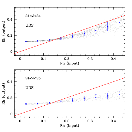
Figure 12: The results of our simulations for $z\sim 7$ galaxies with Sersic profiles of index $n=4$ in the UDS field. The plot shows the comparison between the half–light radius (in arcsec) as measured by SExtractor as a function of the input one. The upper and lower panel refer to different total magnitudes, as reported in the legend. The red line shows the identity relation. The blue points and errorbar shows the average value and the relevant r.m.s. of the output half–light radius. At small sizes the output half light radius is typically larger than the input one due to the convolution with the instrumental PSF carried out during the simulations.

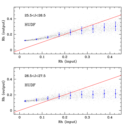
Figure 13: The results of our simulations for $z\sim 7$ galaxies with Sersic profiles of index $n=4$ in the HUDF field. The plot shows the comparison between the half–light radius (in arcsec) as measured by SExtractor as a function of the input one. The upper and lower panel refer to different total magnitudes, as reported in the legend. The red line shows the identity relation. The blue points and errorbar shows the average value and the relevant r.m.s. of the output half–light radius. At small sizes the output half light radius is typically larger than the input one due to the convolution with the instrumental PSF carried out during the simulations.

Fig.14 shows the observed J-band magnitudes versus the measured sizes for simulated (small dots) and observed galaxies (red triangles) at $z\sim 7$ for the EGS, ERS, GDS, P12HUDF and HUDF fields. The solid blue line shows the 50% completeness level for an input simulated profile of disk galaxy. Detailed explanations on the procedure adopted in these simulations can be found in section 4.1.

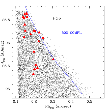
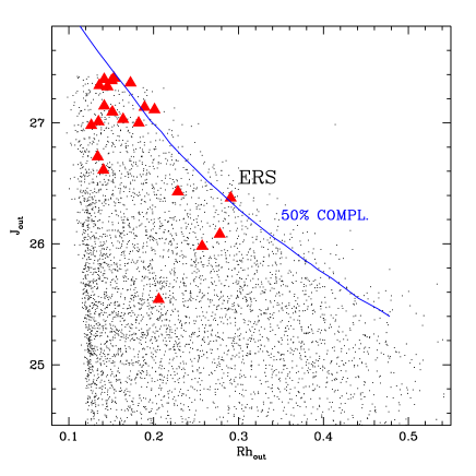
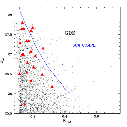
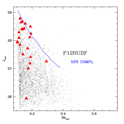
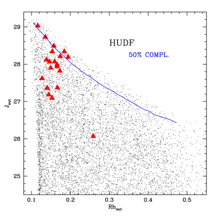
Figure 14: The observed J magnitude vs size of simulated (small dots) and observed galaxies (red triangles) at $z\sim 7$ for the EGS, ERS, GDS, P12HUDF and HUDF fields.

Appendix C Best Fit

The confidence levels for the maximum likelihood analysis of the size distribution on the combined ERS and GDS fields (intermediate sample), and the combined P12HUDF and HUDF fields (faint sample). The best fit is indicated by the magenta point while the green, blue, and red regions define the uncertainties at 68%, 95%, and 99.7% (1,2, and 3 sigma) confidence level, respectively.