On the factorization of chiral logarithms
in the pion form factors

Abstract

The recently proposed hard-pion chiral perturbation theory predicts that the leading chiral logarithms factorize with respect to the energy dependence in the chiral limit. This claim has been successfully tested in the pion form factors up to two loops in chiral perturbation theory. In the present paper we explain this factorization property at two loops and even show that it is valid to all orders for a subclass of diagrams. We also demonstrate that factorization is violated starting at three loops.

1 Introduction

Chiral perturbation theory ($\chi$PT ​) Weinberg:1978kz ; Gasser:1983yg allows one to calculate the momentum and light quark mass dependence of hadronic processes at low energy. It can also be applied to processes in which hard scales are involved, e.g. when baryon or heavy quarks interact with pions. In these cases, however, the range of applicability of the theory is restricted to the kinematical regions in which the momenta of the pions are soft. In ref. Flynn:2008tg Flynn and Sachrajda proposed an interesting argument which, after reinterpreting the effective Lagrangian describing the decay of a heavy meson (the $K$ in that case) into a pion and a lepton-neutrino pair, leads to a prediction of the coefficient of the leading chiral logarithm in $K_{\ell 3}$ decays even for kinematical configurations where the pion is not soft. Subsequently, in a series of papers by Bijnens and collaborators Bijnens:2009yr ; Bijnens:2010ws ; Bijnens:2010jg ; Bijnens:2011bp it has been claimed that the calculation of such a chiral logarithm is possible in more general processes in which the pion is hard. This approach has been referred to as hard pion chiral perturbation theory (H$\pi\chi$PT).

A particularly clear example of a prediction in H$\pi\chi$PT has been provided in ref. Bijnens:2010jg where it has been shown that the scalar and vector form factors of the pion, which have been calculated to two loops in $SU(2)$ $\chi$PT Bijnens:1998fm , in the limit $M_{\pi}^{2}/s\ll 1$ factorize:

$$F_{V,S}(s,M_{\pi}^{2})=\overline{F}_{V,S}(s)\,\big{(}1+\alpha_{V,S}(s)\,L\big{)}+{\cal O}(M^{2})~{}.$$ (1)

Here $s$ is the momentum transfer squared and $L$ stands for the leading chiral logarithm, defined as 

$$L\equiv\frac{M^{2}}{(4\pi F)^{2}}\,\ln\frac{M^{2}}{s}~{}.$$ (2)

$M^{2}$ is proportional to the average up and down quark masses $\hat{m}$ ($M^{2}=2B\hat{m}$) and $F$ is the pion decay constant in the chiral limit:

$$M_{\pi}^{2}=M^{2}+\mathcal{O}(M^{4})~{},\qquad F_{\pi}=F+\mathcal{O}(M^{2})~{}.$$ (3)

$\overline{F}_{V,S}(s)$ denote the form factors for vanishing $u$ and $d$ quark masses . Bijnens and Jemos provide arguments in support of the validity of this factorization property to all orders Bijnens:2010jg . On the other hand a precise formulation of this factorization property is still lacking and it is not clear under what circumstances and for what quantities it holds.

The aim of this paper is to start providing an answer to these questions. In particular we asked ourselves whether factorization of chiral logs for asymptotically small values of the quark masses could be exact, or in other words, a property of QCD. If the latter is true, then this property must emerge also in any effective theory of QCD provided this can deal with the chiral limit. This is the case of $\chi$PT in the limit $M^{2}\ll s\ll\Lambda_{\chi}^{2}$, and indeed the observed factorization in the form factors at two-loop level points in this direction. In the present paper we will analyze the pion form factors in $\chi$PT beyond two loops. We find that the most effective way to attack this problem is to study the dispersion relation for the form factors and apply the chiral counting to this. As we will show, this allows us to formulate a recursive argument and to establish factorization for a subclass of diagrams to all orders in the chiral counting.

We also find, however, that inelastic contributions (three-loop diagrams with a four-pion intermediate state) also generate chiral logs of the order of interest to us and that these violate the factorization property. These diagrams do not fall in the subclass of diagrams which are treated in our recursive argument mentioned above. We conclude that factorization of chiral logs cannot be an exact property of QCD for the pion form factors. If we believe that H$\pi\chi$PT is valid even for (asymptotically) large values of $s$, then this conclusion would be implied by the available results on the meson form factors in the limit of asymptotically large energy. In this limit the pion form factors can be analyzed in the context of perturbative QCD factorization, as shown by Brodsky-Lepage Lepage:1980fj . In their formula the quark masses are neglected, but as discussed by Chen and Stewart Chen:2003fp , it is possible to study the deviation from the chiral limit and in particular to determine the coefficient of the leading chiral log. This chiral log factorizes with respect to the leading Brodsky-Lepage term (but there is no reason to assume that it could factorize for the subleading terms). However, the coefficient of the leading chiral log is different from what is obtained in the low-energy limit.

The paper is organized as follows: in sec. 2 we introduce our notation and briefly discuss the dispersive representation of the pion form factors. In sec. 3 we show how, after applying the chiral counting, one can determine the leading chiral log on the basis of the dispersive representation. Considering only elastic contributions (two-pion intermediate states) we are able to provide a recursive argument and prove factorization of the leading chiral log to all orders. In sec. 4 we discuss the leading inelastic contributions, calculate the chiral log coming from these and show that these violate factorization. In sec. 5 we briefly discuss the papers of Brodsky-Lepage Lepage:1980fj and Chen-Stewart Chen:2003fp and show that these also lead to the same conclusion, namely that factorization of the leading chiral log cannot be exact.

2 Dispersive representation of the pion form factors

We consider the vector and scalar pion form factors, respectively $F_{V}(s)$ and $F_{S}(s)$ and denote them by the common symbol $F(s)$ (unless it is necessary to distinguish them). We normalize the scalar form factor such that  $F_{S}(0)=1$ — for the vector form factor this condition follows from current conservation. Note that this normalization condition (whether automatic or imposed) is inessential to our argument. Both these form factors are analytic functions in the cut plane $[4M_{\pi}^{2},\infty)$ and satisfy a once subtracted dispersion relation of the form

$$F(s)=1+\frac{s}{\pi}\int_{4M_{\pi}^{2}}^{\infty}ds^{\prime}\,\frac{\mathrm{Im\,}F(s^{\prime})}{s^{\prime}(s^{\prime}-s)}~{}.$$ (4)

The subtraction constant is the value of the form factor at zero momentum transfer which is equal to one as mentioned above. In the elastic region unitarity relates the imaginary part of the form factor to the form factor itself and the $\pi\pi$ partial wave with the same quantum numbers:

$$\mathrm{Im\,}F(s)=\sigma(s)\,F(s)\,t^{*}(s)~{},\qquad\sigma(s)=\sqrt{1-\frac{4M_{\pi}^{2}}{s}}~{}.$$ (5)

When $s$ gets larger than the inelastic threshold, additional cuts involving several intermediate pions contribute to the discontinuity. In the subsequent discussion we will consider the form factor which is obtained by solving the dispersion relation with imaginary parts arising only from two-pion intermediate states. We will be able to make a statement about this contribution, provided we consider only two-pion intermediate states also for the $\pi\pi$ scattering amplitude entering the unitarity relation (5). We call this part the elastic contribution, and the rest the “inelastic” part.

$$F(s)=F_{\mathrm{el}}(s)+F_{\mathrm{inel}}(s)~{}.$$ (6)

We stress that this definition is a diagrammatic one. Its precise meaning should become more clear in the following section, in which we will consider only the elastic contribution. The first diagrams contributing to $F_{\mathrm{inel}}(s)$, which start at order $p^{6}$, are discussed in sec. 4.

In the following we will apply the chiral counting to the dispersion relation Gasser:1990bv ; Colangelo:1996hs . It is well-known that if one does so one gets a one-to-one correspondence between direct $\chi$PT calculations and the various chiral orders in the dispersion relation: in other words $\chi$PT provides a perturbative solution to the dispersion relation. This will be the basis of our analysis . Indeed, since $t(s)$ starts at $\mathcal{O}(p^{2})$, knowing the form factor and the $\pi\pi$ partial wave up to a given chiral order means to know $\mathrm{Im\,}F(s)$ at one order higher. If one is then able to perform the dispersive integral, the corresponding real part of the form factor is also obtained. This is a powerful tool which allows us to argue recursively.

The chiral representation contains of course more information than what one gets from the dispersion relation as it also gives the quark mass dependence of subtraction constants. Indeed whenever necessary we will use $\chi$PT to determine chiral logs in subtraction constants. This will be needed in the $\pi\pi$ scattering amplitude, but not for the form factors since with the normalization condition we chose for the form factors (4), the subtraction constant is equal to one and cannot contain any logs.

3 The elastic contribution to $F(s)$

We will now address the question, how leading chiral logarithms can arise from the elastic contribution to the dispersive integral. There are two possible mechanisms to generate terms containing $L$: either one starts from an integrand which does not contain a log of the pion mass and this is produced by the integration over $s^{\prime}$, or the integrand itself contains a chiral log and the dispersive integral determines what function of $s$ multiplies it. We will now discuss these two mechanisms in turn. We stress that, as mentioned in the introduction, we are considering the form factors in the limit $M^{2}\ll s$ and are only interested in terms proportional to $L$: terms of $\mathcal{O}(M^{2})$ without logarithmic enhancement or terms of $\mathcal{O}(M^{2}L)$ are all beyond the accuracy we aim at.

To avoid clutter in the notation in this section we will drop the subscript “el”, $F(s)\mathrel{\widehat{=}}F_{\mathrm{el}}(s)$, as this is the only contribution discussed here.

3.1 Leading chiral logarithms from the dispersive integration

The first possible mechanism is that the leading chiral logarithms are generated by the dispersive integral, i.e. they are produced at the lower integration boundary $s^{\prime}\sim 4M_{\pi}^{2}$, which goes to zero in the chiral limit. In order to investigate this, we must analyze the behavior of the integrand in the regime $s^{\prime}\sim M^{2}\ll s$: we can therefore make use of the standard chiral expansion for the discontinuity of the form factor (5). Expanding both the form factor and the $\pi\pi$ amplitude we can write

$$F(s,M_{\pi}^{2})=1+\mathcal{O}(s)+\mathcal{O}(M^{2})\qquad\mbox{and}\qquad t(s,M_{\pi}^{2})=c_{1}\,M^{2}+c_{2}\,s+\mathcal{O}(s^{2})+\mathcal{O}(M^{4})~{}.$$ (7)

Plugging eq. (7) into eq. (4) we obtain

$$F(s)=1+\frac{s}{\pi}\int_{4M_{\pi}^{2}}^{\infty}ds^{\prime}\frac{\sigma(s^{\prime})}{s^{\prime}(s^{\prime}-s)}\,\Big{(}c_{1}\,M^{2}+c_{2}\,s^{\prime}+\mathcal{O}(p^{4})\Big{)}~{}.$$ (8)

The three terms in brackets in the integrand in eq. (8) generate three types of integrals: the first (the one proportional to $c_{1}$) is the well-known loop function $\bar{J}(s)$ which has the following expansion in $M^{2}/s\ll 1$,

$$\frac{s}{\pi}\int_{4M_{\pi}^{2}}^{\infty}ds^{\prime}\frac{\sigma(s^{\prime})}{s^{\prime}(s^{\prime}-s)}=16\pi\,\bar{J}(s)=\frac{1}{\pi}\left[1+\ln\frac{M^{2}}{-s}+\frac{2M^{2}}{s}\left(1-\ln\frac{M^{2}}{-s}\right)+\mathcal{O}\left(\frac{M^{4}}{s^{2}}\right)\right]~{}.$$ (9)

The remaining two integrals are UV divergent. However, since we are interested in their behaviour close to the lower integration boundary, we can introduce an $M_{\pi}$-independent cut-off $\Lambda^{2}$, which allows us to interchange integration and expansion for small $M$. The second type of integral (the one proportional to $c_{2}$) is then given by

$$\frac{s}{\pi}\int_{4M_{\pi}^{2}}^{\Lambda^{2}}ds^{\prime}\frac{\sigma(s^{\prime})}{(s^{\prime}-s)}=\overline{d}_{1}(s,\Lambda^{2})-\frac{2}{\pi}\,M^{2}\ln\frac{M^{2}}{s}+\mathcal{O}(M^{2})$$ (10)

and the third by

$$\frac{s}{\pi}\int_{4M_{\pi}^{2}}^{\Lambda^{2}}ds^{\prime}\frac{\sigma(s^{\prime})}{s^{\prime}(s^{\prime}-s)}\times\mathcal{O}(p^{4})=\overline{d}_{2}(s,\Lambda^{2})+\mathcal{O}(M^{2})~{}.$$ (11)

With $\mathcal{O}(p^{4})$ we indicate terms proportional to $s^{\prime 2}$, $s^{\prime}M^{2}$ and $M^{4}$, which are all small in the region close to the lower integration boundary. It is easy to see that this further suppression does not allow terms proportional to $L$ (without further powers of $M^{2}$) to be generated. We conclude that the dispersive integral can generate leading chiral logs only from the leading chiral contribution to the integrand. The functions $\overline{d}_{1}(s,\Lambda^{2})$ and $\overline{d}_{2}(s,\Lambda^{2})$ are quark mass independent and contribute to $\overline{F}(s)$ together with the low-energy constants (LECs) which cancel the $\Lambda$-dependence.

Putting all pieces together we conclude that the chiral log generated by the dispersive integration is given by

$$16\pi F^{2}\left(c_{1}-2\,c_{2}\right)L~{}.$$ (12)

The constants $c_{1}$ and $c_{2}$ are related to the leading chiral contributions to the $\pi\pi$ scattering lengths and effective ranges characterizing the threshold expansion

$${\rm Re}\,t_{\ell}^{I}(s)=q^{2\ell}\left(a^{I}_{\ell}+b^{I}_{\ell}q^{2}+\mathcal{O}(q^{4})\right)~{},$$ (13)

where $q^{2}=s/4-M_{\pi}^{2}$ and $I$ and $\ell$ denote isospin and angular momentum, respectively. For the scalar form factor the relevant parameters are $c_{1}=a^{0}_{0}/M^{2}-b_{0}^{0}+\mathcal{O}(M^{2})$ and $c_{2}=b^{0}_{0}/4+\mathcal{O}(M^{2})$ where Gasser:1983yg

$$a^{0}_{0}=\frac{7M^{2}}{32\pi F^{2}}+\mathcal{O}(M^{4})\;,\qquad b_{0}^{0}=\frac{1}{4\pi F^{2}}+\mathcal{O}(M^{2})~{},$$ (14)

leading to

$$\alpha_{S}=16\pi F^{2}\left(c_{1}-2\,c_{2}\right)=16\pi F^{2}\lim_{M^{2}\to 0}\left(\frac{a^{0}_{0}}{M^{2}}-\frac{3b^{0}_{0}}{2}\right)=-\frac{5}{2}~{},$$ (15)

which reproduces the known result Bijnens:1998fm ; Bijnens:2010jg . For the vector form factor we must instead use the parameters: $c_{1}=-(a^{1}_{1})_{|_{M^{2}\to 0}}=-1/(24\pi F^{2})$, and $c_{2}=(a^{1}_{1}/4)_{|_{M^{2}\to 0}}=1/(96\pi F^{2})$, which leads to

$$\alpha_{V}=16\pi F^{2}\left(c_{1}-2\,c_{2}\right)=16\pi F^{2}\lim_{M^{2}\to 0}\left(-\frac{3a^{1}_{1}}{2}\right)=-1~{},$$ (16)

also in agreement with the explicit calculation in refs. Bijnens:1998fm ; Bijnens:2010jg .

For the subsequent discussion it is useful to determine the leading order of $\overline{F}(s)$ in the chiral expansion in powers of $s$ (see also Bissegger:2006ix ). In order to do this, we have to find a function which is analytic in the cut plane $[0,\infty)$ and with the following imaginary part along the cut

$$\lim_{M\to 0}\left[\sigma(s)F^{(0)}(s)\,t^{(2)}(s)\right]=c_{2}\,s~{}.$$ (17)

Such a function is easily found:

$$\overline{F}^{(2)}(s)=s\,\frac{c_{2}}{\pi}\ln\frac{\Lambda_{2}^{2}}{-s}~{},$$ (18)

with $\Lambda_{2}$ an unknown scale. The explicit expressions in the case of the scalar and vector form factors read

$$\overline{F}_{S}^{(2)}(s) = \frac{s}{16\pi^{2}F^{2}}\left[1+\ln\frac{\mu^{2}}{s}+i\pi+16\pi^{2}\ell_{4}^{r}(\mu)\right]$$

$$\overline{F}_{V}^{(2)}(s) = \frac{s}{16\pi^{2}F^{2}}\left[\frac{5}{18}+\frac{1}{6}\ln\frac{\mu^{2}}{s}+\frac{i\pi}{6}-16\pi^{2}\ell_{6}^{r}(\mu)\right]~{},$$ (19)

in agreement with ref. Bijnens:2010jg . The coefficients of the logarithms are indeed correctly reproduced by substituting $c_{2}=(b_{0}^{0}/4)_{|_{M^{2}\to 0}}=1/(16\pi F^{2})$ for the scalar form factor and $c_{2}=(a_{1}^{1}/4)_{|_{M^{2}\to 0}}=1/(96\pi F^{2})$ for the vector one.

3.2 Leading chiral logarithms from the integrand

We shall now discuss whether and how leading chiral logarithms can be generated at higher chiral orders — more specifically, we are interested in terms proportional to $s^{n-1}L$ at order $p^{2n}$. The discussion above made it clear that the behavior of the integrand around the lower limit of integration may only generate a chiral logarithm at $\mathcal{O}(p^{2})$. There is a second mechanism, however, by which chiral logarithms may arise from the dispersive integrals at higher orders, namely if the integrand itself contains a chiral logarithm.

Let us consider the dispersion relation at $\mathcal{O}(p^{4})$ (i.e. the contributions to the form factor at the two-loop level). At this order the integrand has this form

$$\mathrm{Im\,}F^{(4)}(s)=\sigma(s)\left[t^{(4)*}(s)+F^{(2)}(s)\,t^{(2)}(s)\right]$$ (20)

and each of the terms may contain chiral logarithms. We consider first the latter one: $t^{(2)}(s)$ is the tree-level contribution to the $\pi\pi$ scattering amplitude and contains no chiral logarithms, whereas $F^{(2)}(s)$ does, as we have seen above. Expanding in $M^{2}/s$, we can write it as

$$F^{(2)}(s)\,t^{(2)}(s)=\left(\overline{F}^{(2)}(s)+\alpha L\right)\overline{t}^{(2)}(s)+\mathcal{O}(M^{2})~{}.$$ (21)

We can similarly expand $t^{(4)}(s)$,

$$t^{(4)}(s)=\overline{t}^{(4)}(s)+\beta\,sL+\mathcal{O}(M^{2})~{}.$$ (22)

It is easy to realize that the term proportional to $\beta$ would destroy factorization: this vanishes, however, as shown in app. A. We therefore conclude that the only term containing $L$ in eq. (20) has as coefficient exactly the absorptive part of the form factor at one chiral order lower times $\alpha$. As we have discussed above, the solution of the corresponding dispersion relation reads

$$\alpha\,s\,\frac{c_{2}}{\pi}\,\ln\frac{\Lambda_{X}^{2}}{-s}$$ (23)

with $\Lambda_{X}$ an unknown energy scale. We argue, however, that this has to coincide with $\Lambda_{2}$ introduced in eq. (18). From the point of view of $\chi$PT both of these scales are related to LECs in the $\mathcal{O}(p^{4})$ Lagrangian: $\Lambda_{2}$ in particular is the one which appears in the form factor at this order. Since we have just showed that one cannot generate a chiral logarithm by integrating over a local contribution of $\mathcal{O}(p^{4})$ to the $\pi\pi$ scattering amplitude (which is the only other vertex in the dispersion relation), we have to conclude that $\Lambda_{X}=\Lambda_{2}$. We conclude that at two loops we can write the contribution to the form factor as

$$F(s)=\left(1+\overline{F}^{(2)}(s)\right)(1+\alpha L)+\overline{F}^{(4)}(s)+\mathcal{O}(M^{2})+\mathcal{O}(p^{6})~{}.$$ (24)

i.e. in a factorized form, as predicted by H$\pi\chi$PT.

For the elastic contribution to $F(s)$, the same reasoning can be repeated in exactly the same way order by order. At every new step the terms threatening factorization are the contributions to $\mathrm{Im\,}F^{(2n)}$ arising from the $\pi\pi$ scattering amplitude at the same order. A chiral logarithm of the form $s^{n-1}L$ in $t^{(2n)}$ would destroy factorization. In app. A we show that these terms are absent. However, at order $p^{6}$, the four-pion intermediate states contribute to $\mathrm{Im\,}F(s)$ and we will now show that these yield leading chiral logarithms and are responsible for the breakdown of factorization, leading to the three-loop result

$$F(s)=\left(1+\overline{F}^{(2)}(s)+\overline{F}^{(4)}(s)\right)(1+\alpha L)+\alpha_{\rm inel}(s)L+\overline{F}^{(6)}(s)+\mathcal{O}(M^{2})+\mathcal{O}(p^{8})~{}.$$ (25)

Before closing the section we comment on the form factor in the chiral limit: at $\mathcal{O}(p^{4})$ this is given by the solution of the dispersion relation with discontinuity

$$\mathrm{Im\,}\overline{F}^{(4)}(s)=\left[\overline{t}^{(4)*}(s)+\overline{F}^{(2)}(s)\,\overline{t}^{(2)}(s)\right]~{}.$$ (26)

The form factor $\overline{F}^{(4)}(s)$ can be derived from ref. Bijnens:1998fm and given in explicit analytic form. The expression for the scalar form factor, which will be used for the numerical analysis in sec. 4, e.g. reads

$$\overline{F}_{S}^{(4)}(s)=\frac{s^{2}}{F^{4}}\left[\frac{43}{36}\tilde{L}^{2}-\tilde{L}\left(\frac{1}{36N}+\ell_{a}^{r}\right)+\frac{1}{9N}\left(\frac{7}{192}+(\ell_{1}^{r}+2\ell_{2}^{r})+\frac{305}{144N}\right)+r_{S3}^{r}\right]$$ (27)

where $N:=16\pi^{2}$, $\ell_{a}^{r}:=1/3(11\ell_{1}^{r}+7\ell_{2}^{r})+\ell_{4}^{r}$ and $\tilde{L}:=1/N\left(\ln(s/\mu^{2})-i\pi-1\right)$. The $r_{S3}^{r}$ LEC stems from the $\mathcal{O}(p^{6})$ chiral Lagrangian.

4 The contribution from inelastic channels

In the previous section we have shown that the leading chiral logarithms originating from the elastic part factorize. We are now going to show that the $\mathcal{O}(p^{6})$ inelastic contribution leads also to terms proportional to $s^{2}\,L$, i.e. $\alpha_{\rm inel}(s)\neq 0$ in eq. (25), which implies that the factorization hypothesis at the basis of H$\pi\chi$PT is not valid to all orders. We shall now present the details of our calculation.

The lowest order inelastic contribution to $F(s)$ is given by three-loop diagrams with four intermediate pions. We evaluated them by means of the following dispersion relation with the lower integration boundary given by the four-pion threshold:

$$F_{\mathrm{inel}}(s)=\frac{s}{\pi}\int_{16M_{\pi}^{2}}^{\infty}ds^{\prime}\,\frac{\mathrm{Im}\,F_{\mathrm{inel}}(s^{\prime})}{s^{\prime}(s^{\prime}-s)}~{}.$$ (28)

Chiral logarithms are either produced by the dispersive integration or are contained in the integrand. In the chiral counting $\mathrm{Im\,}F_{\mathrm{inel}}$ is of $\mathcal{O}(p^{6})$ and contains a four-particle phase space factor which gives a strong suppression near threshold ( $\Phi_{4}(s)\sim(s-16M_{\pi}^{2})^{7/2}$). Arguing similarly to how we did in sec. 3.1 we conclude that leading chiral logs cannot be generated by the dispersive integration. Therefore we need to concentrate on the integrand.

Due to unitarity, the imaginary part of the form factor has this form

$$\mathrm{Im}\,F_{\mathrm{inel}}(s)=\frac{1}{2}\int d\Phi_{4}(s;p_{1},p_{2},p_{3},p_{4})\,F_{4\pi}\cdot T_{6\pi}^{*}~{},$$ (29)

where $d\Phi_{4}$ is the phase space for four pions of momenta $p_{1},\dots,p_{4}$. $F_{4\pi}$ denotes the current-$4\pi$ vertex and $T_{6\pi}$ is the six-pion scattering amplitude. The three-loop diagrams contributing to $F_{\mathrm{inel}}^{(6)}(s)$ are shown in fig. 1.

Figure 1: Three-loop cut diagrams contributing to the scalar $F_{\mathrm{inel}}(s)$ at order $p^{6}$.

Chiral logarithms are produced by integrations over intermediate momenta with mass-dependent boundaries. We find that, in order to calculate the terms proportional to $L$, we can expand the integrand for small $M$ and keep only the relevant terms. It is then crucial to find a phase space parametrization which allows us to perform analytical integrations after this expansion. We illustrate here a suitable choice for $d\Phi_{4}$.

We reduce the $4$-body phase space defined as

$$d\Phi_{4}(s;p_{1},...,p_{4})=\left(2\pi\right)^{4}\delta^{4}\left(P-\sum_{i=1}^{4}p_{i}\right)\prod_{i=1}^{4}\frac{d^{3}\vec{p}_{i}}{(2\pi)^{3}2p_{i}^{0}}~{}.$$ (30)

with $s=P^{2}$ to the following product of two-body phase space factors (see for example sec. 43 of ref. Beringer:1900zz )

$$d\Phi_{4}(s;p_{1},p_{2},p_{3},p_{4})=d\Phi_{2}(s;q,p_{4})\times d\Phi_{2}(q^{2};k,p_{3})\times d\Phi_{2}(k^{2};p_{1},p_{2})\frac{dk^{2}}{2\pi}\frac{dq^{2}}{2\pi}~{},$$ (31)

where

$$k=p_{1}+p_{2}\,\,,\,\,\,\,\,q=p_{1}+p_{2}+p_{3}\,\,,\,\,\,\,\,p_{1}^{2}=p_{2}^{2}=p_{3}^{2}=p_{4}^{2}=M_{\pi}^{2}~{}.$$ (32)

This gives

$$d\Phi_{4}=\,\frac{1}{(4\pi)^{6}}\frac{\lambda^{1/2}(s,q^{2},M_{\pi}^{2})}{2s}\,\frac{\lambda^{1/2}(q^{2},k^{2},M_{\pi}^{2})}{2q^{2}}\,\frac{\lambda^{1/2}(k^{2},M_{\pi}^{2},M_{\pi}^{2})}{2k^{2}}\,d\Omega_{k}\,d\Omega_{q}\,d\Omega_{s}\,\frac{dq^{2}}{2\pi}\frac{dk^{2}}{2\pi}$$ (33)

in terms of the well-known Källén function $\lambda(x,y,z)\equiv x^{2}+y^{2}+z^{2}-2(xy+xz+yz)$. $\Omega_{s}$ is the solid angle spanned by the unit vector $\hat{q}\equiv\vec{q}/|\vec{q}|$ in the center-of-mass frame of the two final pions. $\Omega_{q}$ is the solid angle spanned by $\hat{k}$ in the frame where $\vec{q}=0$ and $\Omega_{k}$ is the solid angle spanned by $\hat{p}_{1}$ in the frame where $\vec{k}=0$. More details on this phase space parametrization are given in app. C. The advantage of using this representation is that each $\lambda$ function contains $M_{\pi}^{2}$ as an argument, which enables us to expand all factors and perform all the integrations analytically, at least for the diagrams $(a)$, $(b)$, $(c)$ and $(d)$.

The integration range for the kinematic variables $k^{2}$ and $q^{2}$ is determined by the delta function which ensures momentum conservation:

$$4M_{\pi}^{2}\leq k^{2}\leq(\sqrt{q^{2}}-M_{\pi})^{2}\,\,,\,\,\,\,\,9M_{\pi}^{2}\leq q^{2}\leq(\sqrt{s}-M_{\pi})^{2}~{}.$$ (34)

We stress that chiral logarithms stem from both upper and lower integration boundaries due to the functional form of the phase space.

Let us now consider the scalar form factor. For the diagrams $(a)$ to $(d)$ we have been able to determine analytically both the values in the chiral limit and the coefficients of $L$ for $\mathrm{Im\,}F(s)$. The latter ones are given by

$$\delta_{i}\,\frac{s^{2}}{(4\pi F)^{4}}$$ (35)

where the numerical factors are

$$\delta_{a}=-\frac{10}{3}\pi,\quad\delta_{b}=\frac{55}{12}\pi,\quad\delta_{c}=\frac{25}{6}\pi,\quad\delta_{d}=-\frac{9}{4}\pi$$ (36)

For the remaining diagrams the structure is too complicated to perform all integrations analytically. In order to extract the coefficient of the leading chiral logarithm from the remaining diagrams we set up the following procedure. We performed analytical integrations whenever it was possible and the remaining integrations were done numerically. For each diagram we then generated a large number of points within a certain range of values of $M^{2}/s$ and fitted the values of the amplitude minus its chiral limit value with a functional form dictated by $\chi$PT ​. Our optimal choice for the number of points, the range in $M^{2}/s$ and the truncation in powers of $M$ and $s$ of the fit function was determined by our ability to reproduce the coefficients $\delta_{i}$ for the diagrams $(a)$ to $(d)$ within one per cent.

Summing up the contributions from all seven graphs we obtain the coefficient of $L$ in $\mathrm{Im\,}F_{\rm inel}(s)$ at three loops:

$$\delta\,\frac{s^{2}}{(4\pi F)^{4}}\quad{\rm with}\quad\delta=(-0.53\pm 0.05)\,\pi$$ (37)

The error on $\delta$ takes into account the uncertainties both in the numerical integration and in the fit. The pion mass dependence resulting from the sum of the seven diagrams is definitely not compatible with a vanishing coefficient for the chiral logarithm. As a check, we tried to fit with a high degree polynomial in $M^{2}$ but without the leading chiral log and obtained unacceptably high values of $\chi^{2}$.

We checked our results also using the four-body phase-space parametrization in ref. Guo:2011ir . This is not useful to do analytical integrations but it provides an important check of our numerical routine since it involves different kinematic variables and angles compared to our parametrization.

After performing the dispersive integral in eq. (28), our result for $\alpha_{\rm inel}$ is

$$\alpha_{\rm inel}(s)=\left[C(\mu^{2})+\frac{\delta}{\pi}\times\left(\ln{\frac{\mu^{2}}{s}}+i\pi\right)\right]\frac{s^{2}}{(4\pi F)^{4}}$$ (38)

where $C(\mu^{2})$ is a combination of $\mathcal{O}(p^{8})$ LECs which compensates the $\mu$-dependence. Assuming that $C(\mu=1\,{\rm GeV})$ is of natural size, comparing the logarithms from the elastic and inelastic part at three loops, we find that the factorization breaking effect is about 5% in the range of interest for $s$. In fig. 2 we plot the relative contribution of the inelastic log to the total three-loop log (left panel) and the relative contribution of the inelastic log to the sum of the elastic and inelastic log up to three loops (right panel). The LECs are set equal to the values adopted in the analysis of ref. Bijnens:1998fm . We checked that varying them within their phenomenological ranges does not change our conclusions. Comparing the two plots in fig. 2, one can see that for values of $\sqrt{s}$ which are not small compared to $\Lambda_{\chi}$ the three-loop result is not suppressed compared to the two-loop and one-loop results, which is a clear signal of breakdown of chiral power counting.

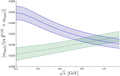
Figure 2: The relative contribution of the inelastic log. The solid line corresponds to $C(\mu=1\,{\rm GeV})=1$ in eq. (38) while the dashed line to $C(\mu=1\,{\rm GeV})=-1$. The bands corresponds to the uncertainty on $\delta$ quoted in eq. (37).

If we go beyond the three-loop level, but still use the chiral counting as a guide, we can write $\alpha_{\rm inel}(s)$ as the following series

$$\alpha_{\rm inel}(s)=\sum_{n=2}^{\infty}\left(\frac{\sqrt{s}}{4\pi F}\right)^{2n}c^{(2n)}(s)$$ (39)

where $c^{(2n)}(s)$ contains $\ln s/\mu^{2}$. Our calculation shows that $c^{(4)}\neq 0$, which indicates that in general $c^{(2n)}\neq 0$ for any $n$. At order $p^{6}$ the inelastic contribution to the chiral log is a small, but non-negligible correction to the factorized one. As long as one remains in the chiral regime $M^{2}\ll s\ll\Lambda_{\chi}^{2}$, factorization of the chiral log does emerge as a property which holds to a good approximation. If, on the other hand we abandon the low-energy region, the chiral counting is not valid anymore and it becomes impossible to even estimate the relative size of the inelastic to the elastic contribution since one should sum the whole series (39) and the analogous one for the elastic part, before being able to draw any conclusion. In fact, if we go to asymptotically large energies, factorization of the chiral log does emerge again as an approximate property, but the origin of it changes completely and the coefficient of the chiral log gets modified, as we are going to discuss in the next section. Evidently, as the energy increases, the inelastic contributions become more and more important and factorization does not hold anymore, until one reaches very high energies where it shows up again in a very different form.

We also stress that at $\mathcal{O}(p^{8})$ in the form factors there will be contributions of four-pion intermediate cuts in the $\pi\pi$ scattering amplitude $t^{(8)}$. These can be additional sources of logarithms.

5 Chiral logs for asymptotic energies

We point out that the factorized form of $F(s)$ conjectured in H$\pi\chi$PT, eq. (1), is also not consistent with QCD factorization for asymptotically large values of $s$. In this regime it is well-known Lepage:1980fj ; Efremov:1979qk ; Chernyak:1983ej that the pion electromagnetic form factor can be written as the following convolution,

$$F_{V}(s)=\frac{F_{\pi}^{2}}{s}\int_{0}^{1}\!dx\,dy\,T(x,y,s)\,\phi_{\pi}(x)\phi_{\pi}(y)\times[1+{\cal O}(\Lambda_{\rm QCD}^{2}/s,M_{\pi}^{2}/s)]~{}.$$ (40)

Here $T$ is a hard scattering kernel which can be calculated in perturbation theory and $\phi_{\pi}$ is the non-perturbative light-cone distribution amplitude (LCDA) for the pion. In the language of Soft-Collinear Effective Theory, this corresponds to the matching of the electromagnetic current onto the leading effective operator built with four collinear quark fields, which has a non-vanishing overlap with symmetric pion states (i.e. containing only energetic modes) Bauer:2002nz .

In ref. Chen:2003fp Chen and Stewart studied the chiral expansion of the vacuum-to-pion matrix element of the bilocal quark field operator defining the $\phi_{\pi}(x)$ in eq. (40). They considered the tower of local axial twist-2 operators $O_{k}^{A,a}$ related to moments of the pion LCDA:

$$\langle\pi^{b}|O_{k}^{A,a}|0\rangle=-iF_{\pi}\delta^{ab}(n\!\cdot\!p_{\pi})^{k+1}\int_{0}^{1}\!dx\,\big{(}1-2x\big{)}^{k}\,\phi_{\pi}(x)~{},$$ (41)

where $n$ is a light-like vector, and proved that for each of these matrix elements the leading chiral log is given just by the one in $F_{\pi}$. Therefore, according to eq. (40) and the result by Chen and Stewart, the leading chiral log in $F_{V}(s)$ does factorize for $s\gg\Lambda_{\rm QCD}^{2}$ but the coefficient $\alpha_{V}$ in eq. (1) is $-2$, not $-1$ as predicted by H$\pi\chi$PT.

6 Conclusions

In this paper we have scrutinized the foundations of hard pion chiral perturbation theory. We did so on the basis of one example, the pion form factors: in this, as well as in other quantities, the leading chiral logs are predicted to factorize in the limit $M^{2}\ll s$. For the form factors, however, this property has been successfully tested by an explicit two-loop calculation in $\chi$PT ​. Our aim was to investigate whether this factorization holds even at higher orders in $\chi$PT ​. Since going beyond two loops within a diagrammatic approach in $\chi$PT is prohibitive, we have based our analysis on dispersion relations and unitarity, and have systematically applied the chiral counting to the dispersive representation. This approach lends itself to a recursive kind of analysis and allowed us to explain why factorization emerges at the two-loop level. Moreover, we have been able to show that for a whole subclass of diagrams this property holds to all orders.

On the other hand, if one considers multipion contributions to the discontinuity of the pion form factor (in short: inelastic contributions), one can see that these also generate chiral logs. We have calculated the coefficient of the leading chiral log in these diagrams at three loops and shown explicitly that these do not factorize. Factorization of the leading chiral logs in the hard pion regime is therefore not an exact property. As long as one remains in the low-energy regime, but takes the quark masses very small ($M^{2}\ll s$) factorization of the chiral logs is valid to a good approximation, as our numerical analysis has shown. As the energy increases, however, the inelastic contributions appear to gradually become more important, until factorization effectively disappears. We conjecture this also because the behaviour of the form factors for asymptotically large energies is known. As Chen and Stewart Chen:2003fp have shown, one can analyze the form factor dependence on the light quark masses in the Brodsky-Lepage formula: they concluded that the chiral log does indeed factorize for the leading term. Nothing is known about subleading terms but there is no reason to assume that the chiral logs would factorize for them too. The coefficient of the chiral log in the leading term has been given explicitly by Chen and Stewart and it is twice as large as what is found at low energy. At intermediate energies some sort of transition between the two regimes must therefore happen, and we see no reason why factorization should be valid in this region.

In the future, we plan to extend this analysis to heavy-light form factors which represent one of the most interesting areas of application of H$\pi\chi$PT.

Appendix A $\pi\pi$ partial waves beyond tree level

Consider the dispersive representation of the $\pi\pi$ partial waves proposed by Roy Roy:1971yg :

$$t^{I}_{\ell}(s)=k^{I}_{\ell}(s)+\sum_{I^{\prime}=0}^{2}\sum_{\ell^{\prime}=0}^{\infty}\int_{4M_{\pi}^{2}}^{\infty}ds^{\prime}K^{II^{\prime}}_{\ell\ell^{\prime}}(s,s^{\prime})\mathrm{Im\,}t^{I^{\prime}}_{\ell^{\prime}}(s^{\prime})~{},$$ (42)

where $I$ and $\ell$ denote isospin and angular momentum respectively and $k^{I}_{\ell}(s)$ is the partial wave projection of the subtraction term

$$k^{I}_{\ell}(s)=a^{I}_{0}\delta_{\ell}^{0}+\frac{s-4M_{\pi}^{2}}{4M_{\pi}^{2}}(2a_{0}^{0}-5a_{0}^{2})\left(\frac{1}{3}\delta_{0}^{I}\delta_{\ell}^{0}+\frac{1}{18}\delta_{1}^{I}\delta_{\ell}^{1}-\frac{1}{6}\delta_{2}^{I}\delta_{\ell}^{0}\right)~{}.$$ (43)

In order to analyze the possible sources for chiral logarithms, we split eq. (42) into the contributions from the $S$- and $P$-waves, the higher partial waves and the integral from a cut-off $\Lambda^{2}$ to infinity:

$$t^{I}_{\ell}(s)=k^{I}_{\ell}(s)+t^{I}_{\ell}(s)_{SP}+d_{\ell}^{I}(s)~{},$$ (44)

where

$$t^{I}_{\ell}(s)_{SP}=\sum_{I^{\prime}=0}^{2}\sum_{\ell^{\prime}=0}^{1}\int_{4M_{\pi}^{2}}^{\Lambda^{2}}ds^{\prime}K^{II^{\prime}}_{\ell\ell^{\prime}}(s,s^{\prime})\mathrm{Im\,}t^{I^{\prime}}_{\ell^{\prime}}(s^{\prime})~{},$$ (45)

and the so called driving terms $d_{\ell}^{I}(s)$ are given by Ananthanarayan:2000ht

$$d_{\ell}^{I}(s)=\sum_{I^{\prime}=0}^{2}\sum_{\ell^{\prime}=2}^{\infty}\int_{4M_{\pi}^{2}}^{\Lambda^{2}}ds^{\prime}K^{II^{\prime}}_{\ell\ell^{\prime}}(s,s^{\prime})\,\mathrm{Im\,}t^{I^{\prime}}_{\ell^{\prime}}(s^{\prime})+\sum_{I^{\prime}=0}^{2}\sum_{\ell^{\prime}=0}^{\infty}\int_{\Lambda^{2}}^{\infty}ds^{\prime}K^{II^{\prime}}_{\ell\ell^{\prime}}(s,s^{\prime})\,\mathrm{Im\,}t^{I^{\prime}}_{\ell^{\prime}}(s^{\prime})~{}.$$ (46)

The expressions of the kernels can be found in ref. Ananthanarayan:2000ht . The subtraction term could in principle contain chiral logarithms but the combination of scattering lengths $2a_{0}^{0}-5a_{0}^{2}$ does not have any Gasser:1983yg . As we are going to show, neither the $S$- and $P$-wave contribution nor the driving terms contain leading chiral logs either.

In the elastic region unitarity relates the imaginary part of the $\pi\pi$ partial wave to its modulus squared:

$$\mathrm{Im}\,t_{l}^{I}(s)=\sigma(s)\,|t_{l}^{I}(s)|^{2}~{}.$$ (47)

The integral over the $S$- and $P$-waves may in principle give rise to chiral logarithms:

$$t^{I}_{\ell}(s)_{SP} = \int_{4M_{\pi}^{2}}^{\Lambda^{2}}ds^{\prime}K^{I0}_{\ell 0}(s,s^{\prime})\left[\frac{1}{2}\,a_{0}^{0}b_{0}^{0}\,s^{\prime}+\frac{1}{16}(b_{0}^{2})^{2}(s^{\prime 2}-8s^{\prime}M^{2})+\mathcal{O}(M^{4})+\mathcal{O}(p^{6})\right]$$

$$+ \int_{4M_{\pi}^{2}}^{\Lambda^{2}}ds^{\prime}K^{I1}_{\ell 1}(s,s^{\prime})\left[\frac{1}{16}\left(a_{1}^{1}\right)^{2}(s^{\prime 2}-8s^{\prime}M^{2})+\mathcal{O}(M^{4})+\mathcal{O}(p^{6})\right]$$

$$+ \int_{4M_{\pi}^{2}}^{\Lambda^{2}}ds^{\prime}K^{I2}_{\ell 0}(s,s^{\prime})\left[\frac{1}{2}a_{0}^{2}b_{0}^{2}s^{\prime}+\frac{1}{16}(b_{0}^{2})^{2}(s^{\prime 2}-8s^{\prime}M^{2})+\mathcal{O}(M^{4})+\mathcal{O}(p^{6})\right]~{}.$$

The partial wave amplitudes needed for the form factors are $t_{0}^{0}(s)$ for $F_{S}(s)$ and $t_{1}^{1}(s)$ for $F_{V}(s)$. Eq. (A) involves integrals of the same type of those discussed in sec. 3.1. We find that for both partial waves the coefficient of $\ln M^{2}/s$ is proportional to

$$\left[2a_{0}^{0}b_{0}^{0}-5a_{0}^{2}b_{0}^{2}\right]-\frac{3M^{2}}{4}\left[2(b_{0}^{0})^{2}+27(a_{1}^{1})^{2}-5(b_{0}^{2})^{2}\right].$$ (49)

Although the individual terms in this combination are of order $M^{2}$, they cancel and leave as leading contribution something of $\mathcal{O}(M^{4})$ and therefore beyond the accuracy of this calculation.

According to the expressions of the kernels, terms proportional to $L$ can be generated only from $\mathrm{Im\,}t(s)$ up to $\mathcal{O}(p^{4})$. Therefore $d_{\ell}^{I}(s)$ cannot produce leading chiral logarithms because there $\mathrm{Im\,}t(s)$ starts at $\mathcal{O}(p^{8})$.

Since the $\pi\pi$ scattering amplitude at tree level and zero momentum vanishes linearly in the chiral limit, it does not contain terms proportional to $L$. Therefore

$$t^{(2)}(s)=\mathcal{O}(M^{2})+\mathcal{O}(s)~{}.$$ (50)

From unitarity, by applying the chiral power counting to eq. (47), it follows that

$$\mathrm{Im}\,t^{(4)}=\sigma(s)\,\lvert t^{(2)}\rvert^{2}\;\;.$$ (51)

Hence also the imaginary part of the partial wave to order $p^{4}$ contains no term proportional to $L$. Using Roy equations (44), we can get the corresponding partial wave $t^{(4)}$ from the imaginary part. Since our previous explicit calculation shows that neither the integration nor the subtraction term produce any unwanted chiral logarithms, the partial wave to next-to-leading order has no terms proportional to $sL$, hence $\beta=0$ in eq. (22). By induction one may reach the same conclusion to all chiral orders provided one does not consider inelastic contributions. This shows that for the partial waves expanded in $M^{2}\ll s$:

$$t^{(2n)}(s)\!=\bar{t}^{(2n)}\!(s)+L\sum_{k=0}^{n-1}\beta_{k}s^{k}M^{2(n-1-k)}+\mathcal{O}(M^{2})$$ (52)

the coefficient $\beta_{n-1}$ vanishes to all orders.

Appendix B Inelastic contributions: explicit expressions of the integrands

We list here the single contributions to the imaginary part of the scalar form factor from the diagrams $(a)$ to $(g)$ in fig. (1), namely

$$\mathrm{Im\,}F_{\mathrm{inel}}^{(i)}(s)=\frac{1}{2}\int d\Phi_{4}(s;p_{1},p_{2},p_{3},p_{4})\,Y_{(i)}~{}.$$ (53)

To express the integrands given here below in terms of the variables of our four-pion phase space parametrization in eq. (33), we refer the reader to app. C. The momenta of the final pions are denoted by $p_{e}$ and $p_{f}$, see fig. 3, and we define $s_{ij}:=p_{i}\cdot p_{j}$ (notice that $s_{ef}=s/2-M^{2}$):

$${Y_{(a)}} = -\frac{5\left(25M^{2}+8s\right)}{24F^{6}}$$ (54)

$${Y_{(b)}} = -\frac{1}{{6F^{6}(M^{2}-q^{2})}}\,\Big{\{}5\Big{[}105M^{4}+2M^{2}(55(s_{12}+s_{13}+s_{23})+20(s_{14}+s_{24}+s_{34})-6s)$$ (55)

$$+8\Big{(}s_{12}(6s_{13}+3s_{14}+6s_{23}+3s_{24}+4s_{34}-s)+s_{23}(4s_{14}+4s_{23}+3s_{24}+3s_{34}-s)$$

$$+s_{13}(3s_{14}+6s_{23}+4s_{24}+3s_{34}-s)+4s_{12}^{2}+4s_{13}^{2}\Big{)}\Big{]}\Big{\}}$$

$${Y_{(c)}} = -\frac{1}{6F^{6}\,(M^{2}-q^{2})}\,\Big{\{}5\Big{(}3M^{2}+2(s_{12}+s_{13}+s_{23})\Big{)}$$ (56)

$$\times\Big{[}3\left(\frac{s}{2}-M^{2}\right)+10\,M^{2}+5(s_{12}+s_{13}+s_{23})+3(s_{14}+s_{24}+s_{34})-s\Big{]}\Big{\}}$$

$${Y_{(d)}} = -\frac{1}{12F^{6}(M^{2}-q^{2})^{2}}\Big{\{}\Big{[}15M^{4}+20M^{2}(s_{12}+s_{13}+s_{23})$$ (57)

$$+4\,\Big{(}3(s_{12}^{2}+s_{13}^{2}+s_{23}^{2})+2(s_{13}s_{12}+s_{23}s_{12}+s_{13}s_{23})\Big{)}\Big{]}$$

$$\times(14M^{2}+10(s_{12}+s_{13}+s_{23})+6(s_{14}+s_{24}+s_{34})+s)\Big{\}}$$

$${Y_{(e)}} = \frac{5}{4\,F^{6}[M^{2}-(p_{1}+p_{2}-p_{e})^{2}]}\Big{\{}2M^{2}(5\,s_{12}+3(s_{ef}-s_{1e}-s_{2e}-s_{1f}-s_{2f}+s_{34})$$ (58)

$$+4(s_{13}+s_{14}+s_{23}+s_{24}-s_{3e}-s_{4e}-s_{3f}-s_{4f}))+4\Big{[}s_{12}\,(s_{34}+s_{ef}-s_{1f}-s_{2f}$$

$$+2(s_{13}+s_{14}+s_{23}+s_{24}-s_{3e}-s_{4e}-s_{3f}-s_{4f}))-(s_{1e}+s_{2e})(s_{13}+s_{14}+s_{23}$$

$$+s_{24}+s_{34}+s_{ef}-s_{3e}-s_{4e}-s_{1f}-s_{2f}-s_{3f}-s_{4f})\Big{]}+11\,M^{4}\Big{\}}$$

$$Y_{(f)} = \frac{1}{2F^{6}[M^{2}-(p_{1}+p_{3}+p_{4})^{2}](M^{2}-q^{2})}\Big{\{}\Big{[}15\,M^{4}+10\,M^{2}(s_{12}+2s_{13}+s_{14}+s_{23}+s_{34})$$ (59)

$$+4\Big{(}s_{13}(s_{12}+3s_{13}+s_{23})+\,s_{14}\,(s_{12}+s_{13}+3s_{23})+s_{34}(3s_{12}+s_{13}+s_{23})\,\Big{)}\Big{]}$$

$$\times(3M^{2}+2s_{12}+2s_{23}+2s_{24}-3s)\Big{\}}$$

$${Y_{(g)}} = -\frac{1}{2F^{6}(M^{2}-q^{2})[M^{2}-(p_{1}+p_{2}-p_{e})^{2}]}\Big{\{}\!-55\,M^{6}-10M^{4}(10s_{12}+7s_{13}+4s_{14}-3s_{1e}$$ (60)

$$-3s_{1f}+7s_{23}+4s_{24}-3s_{2e}-3s_{2f}+3s_{34}-4s_{3e}-4s_{3f}-4s_{4e}-4s_{4f}+3s_{ef})$$

$$-20\,M^{2}\Big{[}3s_{12}^{2}+s_{12}(5s_{13}+4s_{14}-s_{1e}-2s_{1f}+5s_{23}+4s_{24}-s_{2e}-2s_{2f}+2s_{34}-4s_{3e}$$

$$-4s_{3f}-4s_{4e}-4s_{4f}+2s_{ef})+s_{13}^{2}+s_{23}^{2}-s_{14}\,s_{1e}+s_{1e}\,s_{1f}+s_{14}\,s_{23}-2s_{1e}\,s_{23}$$

$$-s_{1f}\,s_{23}-s_{1e}\,s_{24}+s_{23}\,s_{24}-s_{14}\,s_{2e}+s_{1f}\,s_{2e}-2s_{23}\,s_{2e}-s_{24}\,s_{2e}+s_{1e}\,s_{2f}-s_{23}\,s_{2f}$$

$$+s_{2e}\,s_{2f}-s_{1e}\,s_{34}+s_{23}\,s_{34}-s_{2e}\,s_{34}+s_{1e}\,s_{3e}-s_{23}\,s_{3e}+s_{2e}\,s_{3e}+s_{1e}\,s_{3f}-s_{23}\,s_{3f}$$

$$+s_{2e}\,s_{3f}+s_{1e}\,s_{4e}-s_{23}\,s_{4e}+s_{2e}\,s_{4e}+s_{1e}\,s_{4f}-s_{23}\,s_{4f}+s_{2e}\,s_{4f}-s_{1e}\,s_{ef}+s_{23}\,s_{ef}$$

$$-s_{2e}\,s_{ef}+s_{13}\,(s_{14}-2s_{1e}-s_{1f}+2s_{23}+s_{24}-2s_{2e}-s_{2f}+s_{34}-s_{3e}-s_{3f}-s_{4e}-s_{4f}$$

$$+s_{ef})\Big{]}-8\Big{[}3s_{12}^{2}(2s_{13}+2s_{14}-s_{1f}+2s_{23}+2s_{24}-s_{2f}+s_{34}-2s_{3e}-2s_{3f}-2s_{4e}$$

$$-2s_{4f}+s_{ef})+s_{12}(s_{13}-s_{1e}+s_{23}-s_{2e})(2s_{13}+2s_{14}-s_{1f}+2s_{23}+2s_{24}-s_{2f}+s_{34}$$

$$-2s_{3e}-2s_{3f}-2s_{4e}-2s_{4f}+s_{ef})-s_{13}^{2}\,(2s_{1e}+s_{2e})+s_{13}\,\Big{(}\!-s_{14}(s_{1e}+2s_{2e})$$

$$+s_{2e}\,(2s_{1f}-3s_{23}-2s_{24}+2s_{2f}-2s_{34}+s_{3e}+2s_{3f}+2s_{4e}+s_{4f}-2s_{ef})$$

$$+s_{1e}\,(2s_{1f}-3s_{23}-s_{24}+2s_{2f}-2s_{34}+2s_{3e}+s_{3f}+s_{4e}+2s_{4f}-2s_{ef})\Big{)}$$

$$+s_{23}\,\Big{(}\!s_{1e}(2s_{1f}-s_{23}-2s_{24}+2s_{2f}-2s_{34}+s_{3e}+2s_{3f}+2s_{4e}+s_{4f}-2s_{ef})$$

$$+s_{2e}(2s_{1f}-2s_{23}-s_{24}+2s_{2f}-2s_{34}+2s_{3e}+s_{3f}+s_{4e}+2s_{4f}-2s_{ef})$$

$$-s_{14}(2s_{1e}+s_{2e})\Big{)}\Big{]}\Big{\}}$$

Appendix C Four-pion phase space and related Lorentz transformations

In order to perform the integral over the four-pion phase space in eq. (33) we need to express all the dot products $p_{i}\cdot p_{j}$ entering the Feynman rules for the cut diagrams in terms of our integration variables. We define angles in the following frames: $\Sigma_{s}$, which is the center of mass frame (CMF) of the two final pions, $\Sigma_{q}$, which is the CMF of the particles $p_{1}$, $p_{2}$ and $p_{3}$, and $\Sigma_{k}$ which is the CMF of the particles $p_{1}$and $p_{2}$. The labels of the particle momenta are explained in fig. 3.

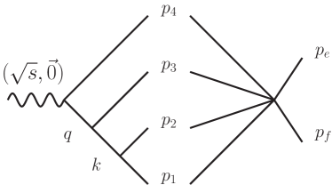
Figure 3: The kinematic invariants corresponding to our choice of parametrization: $s=(p_{1}+p_{2}+p_{3}+p_{4})^{2}$, $q^{2}=(p_{1}+p_{2}+p_{3})^{2}$ and $k^{2}=(p_{1}+p_{2})^{2}$.

Figure 4: Our choice of reference frames and angles.

The angles and the corresponding reference frames are shown in fig. 4. The latter ones are connected by the following Lorentz transformations

$$\Sigma_{s}\quad\mathop{\leftarrow}\limits^{\Lambda_{1}}\quad\Sigma_{q}\quad\mathop{\leftarrow}\limits^{\Lambda_{2}}\quad\Sigma_{k}\,\,.$$ (61)

These are given by

$$\Lambda_{1}=\left(\begin{array}[]{cccc}\frac{s+q^{2}-M^{2}}{2\sqrt{q^{2}}\sqrt{s}}&0&\frac{\lambda^{1/2}\left(s,q^{2},M^{2}\right)}{2\sqrt{q^{2}}\sqrt{s}}&0\\ 0&1&0&0\\ \frac{\lambda^{1/2}\left(s,q^{2},M^{2}\right)}{2\sqrt{q^{2}}\sqrt{s}}&0&\frac{s+q^{2}-M^{2}}{2\sqrt{q^{2}}\sqrt{s}}&0\\ 0&0&0&1\end{array}\right)$$ (62)

and by

$$\Lambda_{2}=\left(\begin{array}[]{cccc}\frac{k^{2}+q^{2}-M^{2}}{2\sqrt{k^{2}}\sqrt{q^{2}}}&\frac{\lambda^{1/2}\left(k^{2},q^{2},M^{2}\right)}{2\sqrt{k^{2}}\sqrt{q^{2}}}\sin\phi&\frac{\lambda^{1/2}\left(k^{2},q^{2},M^{2}\right)}{2\sqrt{k^{2}}\sqrt{q^{2}}}\cos\phi&0\\ 0&\cos\phi&-\sin\phi&0\\ \frac{\lambda^{1/2}\left(k^{2},q^{2},M^{2}\right)}{2\sqrt{k^{2}}\sqrt{q^{2}}}\cos\theta_{k}&\frac{k^{2}+q^{2}-M^{2}}{2\sqrt{k^{2}}\sqrt{q^{2}}}\sin\phi\cos\theta_{k}&\frac{k^{2}+q^{2}-M^{2}}{2\sqrt{k^{2}}\sqrt{q^{2}}}\cos\phi\cos\theta_{k}&-\sin\theta_{k}\\ \frac{\lambda^{1/2}\left(k^{2},q^{2},M^{2}\right)}{2\sqrt{k^{2}}\sqrt{q^{2}}}\sin\theta_{k}&\frac{k^{2}+q^{2}-M^{2}}{2\sqrt{k^{2}}\sqrt{q^{2}}}\sin\phi\sin\theta_{k}&\frac{k^{2}+q^{2}-M^{2}}{2\sqrt{k^{2}}\sqrt{q^{2}}}\cos\phi\sin\theta_{k}&\cos\theta_{k}\end{array}\right)\,,$$ (63)

with the usual Källén function $\lambda(x,y,z)=x^{2}+y^{2}+z^{2}-2xy-2xz-2yz$. Now we give the momentum vectors in the frames where they have the simplest form. We define the four-vectors $p_{1}$ and $p_{2}$ in the frame $\Sigma_{k}$ as follows

$$p_{1}^{\prime\prime}=\frac{\sqrt{k^{2}}}{2}\left(\begin{array}[]{c}1\\ 0\\ \sigma(k^{2})\sin\theta_{a}\\ \sigma(k^{2})\cos\theta_{a}\end{array}\right)\,\,,\quad p_{2}^{\prime\prime}=\frac{\sqrt{k^{2}}}{2}\left(\begin{array}[]{c}1\\ 0\\ -\sigma(k^{2})\sin\theta_{a}\\ -\sigma(k^{2})\cos\theta_{a}\end{array}\right)\,\,,$$ (64)

with $\sigma(x)=\sqrt{1-4M_{\pi}^{2}/x}$. We give the four-vector $p_{3}$ in the frame $\Sigma_{q}$

$$p_{3}^{\prime}=\left(\begin{array}[]{c}\frac{q^{2}-k^{2}+M^{2}}{2\sqrt{q^{2}}}\\ 0\\ -\frac{\lambda^{1/2}\left(q^{2},k^{2},M^{2}\right)}{2\sqrt{q^{2}}}\cos\theta_{k}\\ -\frac{\lambda^{1/2}\left(q^{2},k^{2},M^{2}\right)}{2\sqrt{q^{2}}}\sin\theta_{k}\end{array}\right)$$ (65)

and the four-vectors $p_{4}$, $p_{e}$ and $p_{f}$ in $\Sigma_{s}$

$$p_{4}=\left(\begin{array}[]{c}\frac{s-q^{2}+M^{2}}{2\sqrt{s}}\\ 0\\ -\frac{\lambda^{1/2}\left(s,q^{2},M^{2}\right)}{2\sqrt{s}}\\ 0\end{array}\right)\,,\quad$$ (70)

$$p_{e}=\frac{\sqrt{s}}{2}\left(\begin{array}[]{c}1\\ \sigma(s)\sin\theta_{e}\cos\phi_{e}\\ \sigma(s)\sin\theta_{e}\sin\phi_{e}\\ \sigma(s)\cos\theta_{e}\end{array}\right)\,,\quad p_{f}=\frac{\sqrt{s}}{2}\left(\begin{array}[]{c}1\\ -\sigma(s)\cos\phi_{e}\sin\theta_{e}\\ -\sigma(s)\sin\phi_{e}\sin\theta_{e}\\ -\sigma(s)\cos\theta_{e}\end{array}\right)\,.$$ (79)

After transforming all these momentum vectors onto the same frame, all Lorentz invariants are written as functions of the seven phase space variables $k^{2}$, $q^{2}$, $\theta_{k}$, $\theta_{a}$, $\theta_{e}$, $\phi$ and $\phi_{e}$.

References

- (1) S. Weinberg, Phenomenological Lagrangians, Physica A96 (1979) 327.
- (2) J. Gasser and H. Leutwyler, Chiral Perturbation Theory to One Loop, Ann. Phys. 158 (1984) 142.
- (3) RBC Collaboration, UKQCD Collaboration Collaboration, J. Flynn and C. Sachrajda, SU(2) chiral perturbation theory for K(l3) decay amplitudes, Nucl.Phys. B812 (2009) 64–80, [arXiv:0809.1229].
- (4) J. Bijnens and A. Celis, Decays in SU(2) Chiral Perturbation Theory, Phys.Lett. B680 (2009) 466–470, [arXiv:0906.0302].
- (5) J. Bijnens and I. Jemos, Hard Pion Chiral Perturbation Theory for and Formfactors, Nucl.Phys. B840 (2010) 54–66, [arXiv:1006.1197].
- (6) J. Bijnens and I. Jemos, Vector Formfactors in Hard Pion Chiral Perturbation Theory, Nucl. Phys. B846 (2011) 145–166, [arXiv:1011.6531].
- (7) J. Bijnens and I. Jemos, Chiral Symmetry and Charmonium Decays to Two Pseudoscalars, Eur.Phys.J. A47 (2011) 137, [arXiv:1109.5033].
- (8) J. Bijnens, G. Colangelo, and P. Talavera, The vector and scalar form factors of the pion to two loops, JHEP 05 (1998) 014, [hep-ph/9805389].
- (9) G. P. Lepage and S. J. Brodsky, Exclusive Processes in Perturbative Quantum Chromodynamics, Phys.Rev. D22 (1980) 2157.
- (10) J.-W. Chen and I. W. Stewart, Model independent results for SU(3) violation in light cone distribution functions, Phys.Rev.Lett. 92 (2004) 202001, [hep-ph/0311285].
- (11) J. Gasser and U. G. Meissner, Chiral expansion of pion form-factors beyond one loop, Nucl.Phys. B357 (1991) 90–128.
- (12) G. Colangelo, M. Finkemeier, and R. Urech, Tau decays and chiral perturbation theory, Phys.Rev. D54 (1996) 4403–4418, [hep-ph/9604279].
- (13) J. F. Donoghue, On the marriage of chiral perturbation theory and dispersion relations, hep-ph/9506205.
- (14) J. Gasser and A. Zepeda, APPROACHING THE CHIRAL LIMIT IN QCD, Nucl.Phys. B174 (1980) 445.
- (15) J. Gasser, Hadron Masses and Sigma Commutator in the Light of Chiral Perturbation Theory, Annals Phys. 136 (1981) 62.
- (16) M. Bissegger and A. Fuhrer, Chiral logarithms to five loops, Phys.Lett. B646 (2007) 72–79, [hep-ph/0612096].
- (17) Particle Data Group Collaboration, J. Beringer et. al., Review of Particle Physics (RPP), Phys.Rev. D86 (2012) 010001.
- (18) F.-K. Guo, B. Kubis, and A. Wirzba, Anomalous decays of eta’ and eta into four pions, Phys.Rev. D85 (2012) 014014, [arXiv:1111.5949].
- (19) A. Efremov and A. Radyushkin, Factorization and Asymptotical Behavior of Pion Form-Factor in QCD, Phys.Lett. B94 (1980) 245–250.
- (20) V. Chernyak and A. Zhitnitsky, Asymptotic Behavior of Exclusive Processes in QCD, Phys.Rept. 112 (1984) 173.
- (21) C. W. Bauer, S. Fleming, D. Pirjol, I. Z. Rothstein, and I. W. Stewart, Hard scattering factorization from effective field theory, Phys.Rev. D66 (2002) 014017, [hep-ph/0202088].
- (22) S. Roy, Exact integral equation for pion-pion scattering involving only physical region partial waves, Phys. Lett. B 36 (1971) 353.
- (23) B. Ananthanarayan, G. Colangelo, J. Gasser, and H. Leutwyler, Roy equation analysis of scattering, Phys.Rept. 353 (2001) 207–279, [hep-ph/0005297].