REVISITING THE COSMIC STAR FORMATION HISTORY: CAUTION ON THE UNCERTAINTIES IN DUST CORRECTION AND STAR FORMATION RATE CONVERSION

Abstract

The cosmic star formation rate density (CSFRD) has been observationally investigated out to redshift $z\simeq 10$. However, most of the theoretical models for galaxy formation underpredict the CSFRD at $z\gtrsim 1$. Since the theoretical models reproduce the observed luminosity functions (LFs), luminosity densities (LDs), and stellar mass density at each redshift, this inconsistency does not simply imply that theoretical models should incorporate some missing unknown physical processes in galaxy formation. Here, we examine the cause of this inconsistency at UV wavelengths by using a mock catalog of galaxies generated by a semi-analytic model of galaxy formation. We find that this inconsistency is due to two observational uncertainties: the dust obscuration correction and the conversion from UV luminosity to star formation rate (SFR). The methods for correction of obscuration and SFR conversion used in observational studies result in the overestimation of the CSFRD by $\sim 0.1$–$0.3$ dex and $\sim 0.1$–$0.2$ dex, respectively, compared to the results obtained directly from our mock catalog. We present new empirical calibrations for dust attenuation and conversion from observed UV LFs and LDs into the CSFRD.

¹ Astronomy Data Center, National Astronomical Observatory of Japan, Mitaka, Tokyo 181-8588, Japan; kobayashi@cosmos.phys.sci.ehime-u.ac.jp ² Research Center for Space and Cosmic Evolution, Ehime University, Bunkyo-cho, Matsuyama 790-8577, Japan ³ Kavli Institute for Particle Astrophysics and Cosmology, Department of Physics and SLAC National Accelerator Laboratory,
Stanford University, Stanford, CA 94305, USA ⁴ College of General Education, Osaka Sangyo University, 3-1-1 Nakagaito Daito, Osaka 574-8530, Japan

1. Introduction

The cosmic star formation rate density (CSFRD), $\dot{\rho}_{\star}$, is one of the most fundamental quantities that reveals how present galaxies were formed and evolved in the universe. It has been probed observationally since the seminal works of Lilly et al. (1996) and Madau et al. (1996, 1998) using various star formation rate (SFR) indicators such as luminosities of the stellar continuum at the rest-frame ultraviolet (UV) and nebular emission lines (e.g., H$\alpha$). Various observational results are compiled in Hopkins (2004; H04) and Hopkins & Beacom (2006; HB06), in which the cosmology, stellar initial mass function (IMF), and dust obscuration correction are unified. The best-fit CSFRD function using these results has been widely utilized not only in observational studies (e.g., Karim et al. 2011) but also in theoretical studies (e.g., Coward et al. 2008; Kistler et al. 2009; Tominaga et al. 2011; Wang & Dai 2011).

The CSFRD at $z\lesssim 1$ has been confirmed by various SFR indicators obtained from wide-field surveys such as the Galaxy Evolution Explorer (e.g., Wyder et al. 2005; Robotham & Driver 2011). Its characteristic feature is a rapid increase with redshift ($\dot{\rho}_{\star}\propto(1+z)^{3-4}$ at $z\lesssim 1$; H04 and references therein). Thus, the CSFRD at $z\sim 1$ is an order of magnitude higher than that in the local universe. In contrast, the CSFRD is still uncertain in the higher redshift range (i.e., $z\gtrsim 1$) where popular SFR indicators include the rest-frame UV continuum stellar emission and infrared (IR) dust emission. This uncertainty is due to uncertainties in the estimation of the CSFRD from observed data: the dust obscuration correction for the UV continuum, contamination from the old stellar population to the IR luminosity, estimation of the total IR luminosity, the faint-end slope of the luminosity function (LF), and the conversion factor from luminosity into SFR. These uncertainties result in the well-known inconsistencies in some physical quantities between direct measurements and values inferred from the HB06 CSFRD function such as stellar mass density (SMD; $\rho_{\star}$: e.g., Wilkins et al. 2008; Choi & Nagamine 2012; Benson 2012), core-collapse supernova rate (e.g., Horiuchi et al. 2011; see also Botticella et al. 2012 who report there is no inconsistency in the local 11 Mpc volume), and extragalactic background light (e.g., Raue & Meyer 2012).

The CSFRD has also been calculated theoretically using galaxy formation models: hydrodynamic simulation (e.g., Nagamine et al. 2006) or semi-analytic models (e.g., Cole et al. 2001; Nagashima & Yoshii 2004; Benson 2012). In these models, a galaxy-by-galaxy basis calculation is executed based on a detailed hierarchical structure formation scenario. Therefore, the CSFRD at a certain redshift can be calculated by simply integrating the SFR of each galaxy at that redshift. Although these theoretical models reproduce reasonably well the observed LFs and the luminosity densities (LDs) at the rest-frame wavelength dominated by stellar emission, and the SMD at both local and high $z$, most underpredict the CSFRD compared to that estimated observationally (e.g., Nagashima & Yoshii 2004; Nagashima et al. 2005; Lacey et al. 2011; Benson 2012). While the underprediction of the CSFRD might be attributed to some missing unknown physical processes of galaxy formation and evolution, it is worth investigating whether or not the uncertainties in estimating the CSFRD from directly observed data could be the origin of the disagreement.

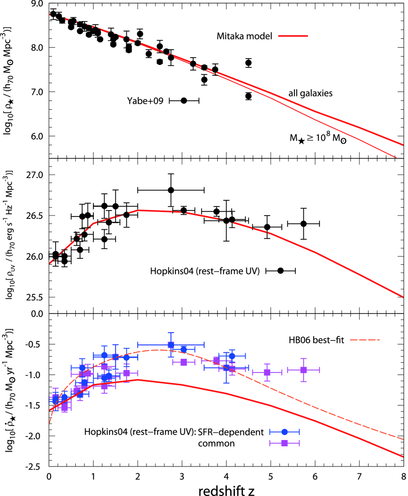
Figure 1.— Redshift evolution of the SMD (top), the rest-frame UV (i.e., $\lambda=1500$–2800 Å) LD (middle), and the CSFRD (bottom). The solid curves in each panel are the predictions of the Mitaka model. The thin solid curve in the top panel is the SMD for model galaxies with $M_{\star}\geq 10^{8}\ M_{\odot}$. The dashed curve in the bottom panel is the best-fit Cole et al. (2001) functional form to the H04 $\dot{\rho}_{\star}$. The symbols with error bars are observational data. The observational data shown in the top panel are compiled in Yabe et al. (2009) and those in the middle and bottom panels are from H04, respectively. In the bottom panel, the boxes (circles) are evaluated using a common (SFR-dependent) obscuration correction from H04 for the same observed data plotted in the middle panel.

Here, we examine the CSFRD through a comparison of the observational data compiled in H04 with the mock catalog of galaxies generated by one of the semi-analytic models for galaxy formation, the so-called Mitaka model (Nagashima & Yoshii 2004; see also Nagashima et al. 2005). The Mitaka model reproduces various kinds of observations not only for local galaxies including the stellar continuum LFs (Nagashima & Yoshii 2004) but also for high-$z$ Lyman-break galaxies and Ly$\alpha$ emitters (Kashikawa et al. 2006; Kobayashi et al. 2007, 2010). In this paper, we focus on the rest-frame UV continuum luminosity as an SFR indicator; this is usually applied to galaxies in the high-$z$ universe (e.g., Madau et al. 1996, 1998). Investigation of other SFR indicators, such as the rest-frame IR continuum emitted by interstellar dust, will be the subject of future work.

As shown in the top and middle panels of Figure 1, the Mitaka model reproduces well the measured SMD, $\rho_{\star}$, and LD at rest-frame UV wavelengths, $\rho_{\mathrm{UV}}$, which have not been corrected for interstellar dust attenuation, in the redshift range $z=0$–$6$. However, the model prediction for the CSFRD is underestimated at $z\gtrsim 1$ by a factor of $\sim 2$–3 (i.e., $\sim 0.3$–0.5 dex) relative to the median value of $\dot{\rho}_{\star}$ compiled in H04 as shown in the bottom panel of Figure 1. It should be emphasized that these H04 CSFRD data are calculated using the same observational UV LDs plotted in the middle panel of Figure 1, and which are reasonably reproduced by our model. Moreover, our CSFRD is consistent with the upper limit for $\dot{\rho}_{\star}$ given by Strigari et al. (2005) estimated from an upper limit on the diffuse supernova neutrino background with Super-Kamiokande. In this paper we show that the underestimation of the Mitaka model relative to the H04 CSFRD can be fully attributed to two observational uncertainties, the dust obscuration correction and the SFR conversion used in observational studies. Therefore the underestimation using theoretical galaxy formation models relative to the H04 CSFRD does not necessarily imply that these models should incorporate some missing unknown physical processes.

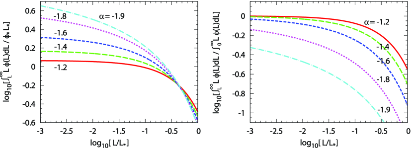
Figure 2.— LD contribution from galaxies brighter than the horizontal axis of $L/L_{\ast}$ calculated using the Schechter function with various faint-end slopes of the LF. As on the figure, the solid, long-dashed, short-dashed, dotted, and dash-dotted curves are for $\alpha=-1.2$, $-1.4$, $-1.6$, $-1.8$, and $-1.9$, respectively. The left and right panels are the LD normalized by $\phi_{\ast}L_{\ast}$ and the total LD, respectively.

The paper is organized as follows. In Section 2, we list the uncertainties in estimating the CSFRD from observed UV LFs. In Section 3, we describe the key prescriptions of the Mitaka model relating to the observational uncertainties in estimating the CSFRD. Then we compare the model results with the observed LFs, LDs, and CSFRD in the redshift range $z=0$–10 in Section 4. We summarize our work in Section 5, where we also provide a discussion which includes a new formula for the obscuration correction at rest-frame UV wavelengths in Section 5. Throughout this paper, we adopt the 737 cosmology, i.e., $H_{0}=70~{}\mathrm{km\ s^{-1}\ Mpc^{-1}}$ (i.e., $h_{70}\equiv h/0.7=1$), $\Omega_{M}=0.3$, and $\Omega_{\Lambda}=0.7$, and a Salpeter IMF with a mass range of $0.1$–$60~{}M_{\odot}$. All magnitudes are expressed in the AB system and the wavelengths are given in the rest frame unless otherwise stated.

2. Uncertainties in Estimating the Cosmic Star Formation Rate Density

In the process of estimating the CSFRD at a certain redshift from observational data of galaxies, the basic direct observable quantities are the luminosities which can be used as SFR indicators. Luminosities can be converted into the CSFRD via the following processes. First, the observed luminosities are corrected for dust attenuation in order to obtain intrinsic luminosities which are expected to correlate more directly with the SFR. Next, the LF is constructed from the data corrected for dust obscuration. Since the data are flux-limited samples, the main uncertainty in the shape of the LF lies in the faint-end slope index. Next, the LD is derived by integrating the LF. These processes can be interchanged if a luminosity-independent obscuration correction is adopted. Finally, the LD is converted to the CSFRD using the SFR conversion factor. Thus, uncertainties may arise from (1) the faint-end slope of the LF, (2) the conversion factor from luminosity into SFR, and (3) the dust obscuration correction.

There are other uncertainties in the estimation of the CSFRD such as the limiting luminosity to which LF is integrated (e.g., Reddy & Steidel 2009), the IMF (e.g., HB06), and leakage of ionizing photons (e.g., Relaño et al. 2012). As the limiting luminosity and IMF are calibrated in a common fashion in H04, we do not need to examine these uncertainties here. We can also neglect the uncertainty caused by the leakage of ionizing photons because we treat the UV continuum luminosity as an SFR indicator. Hence, here we briefly describe the three uncertainties described in the previous paragraph, focusing on the UV continuum luminosity as an SFR indicator.

2.1. Faint-end Slope of the Luminosity Function

In general, the uncertainty in the faint-end slope of the LF, $\alpha$, leads that of the integrated LD. It is more significant at high $z$ simply because only bright galaxies are detected at high $z$ in flux-limited surveys and thus the uncertainty in $\alpha$ becomes larger.

Figure 2 shows the LDs for various $\alpha$ as a function of minimum luminosity. We normalize the LDs by the characteristic luminosity $L_{\ast}$ and number density $\phi_{\ast}$ and adopt the Schechter function form for the LF. For a typical value of $\alpha\sim-1.5$ in the UV LFs at $z=0$–6 (e.g., Oesch et al. 2010), the uncertainty of $\Delta\alpha=\pm 0.3$ results in $\sim 0.2$–0.3 dex (a factor of $\sim 1.6$–2) uncertainty in the LD integrated to $\log_{10}\left(L/L_{\ast}\right)\sim-3$. If this uncertainty fluctuates randomly to positive or negative values, it may be the origin of the dispersion in the LDs at each redshift as shown in the middle panel of Figure 1.

However, because the UV LD calculated from the Mitaka model lies around the median value of the observed UV LDs, the uncertainty in $\alpha$ is not the origin of the systematic underestimation of the CSFRD calculated using the Mitaka model compared to that of H04; hence, we do not treat this uncertainty further here.

2.2. Conversion from Stellar Continuum Luminosity into SFR

The intrinsic (i.e., without dust attenuation) stellar continuum luminosity at UV wavelengths, $L_{\nu,\mathrm{UV}}^{\mathrm{int}}$, is one of the best SFR indicators. This is because it is dominated by stellar radiation from recently formed massive stars and rest-frame UV photons from redshift $z=3$–10 to optical or near-IR in the observer frame at which we can observe most efficiently with current telescopes.

In observational studies, the conversion factor from $L_{\nu,\mathrm{UV}}^{\mathrm{int}}$ to SFR, $C_{\mathrm{SFR}}$, given by Kennicutt (1998; hereafter, K98) has been widely utilized:

$$C_{\mathrm{SFR}}^{\mathrm{K98}}\equiv\mathrm{SFR}/L_{\nu,\mathrm{UV}}^{\mathrm{int}}=1.4\times 10^{-28}\ M_{\odot}\ \mathrm{yr^{-1}\ (erg\ s^{-1}\ Hz^{-1})^{-1}}.$$

H04 and HB06 also adopted $C_{\mathrm{SFR}}^{\mathrm{K98}}$. However, it should be noted that, as explicitly stated in K98, the linear relation holds only for galaxies which continuously form stars over timescales of 100 Myr or longer, have solar metallicity, and the Salpeter IMF in the mass range $0.1$–$100~{}M_{\odot}$ (see also Madau et al. 1998).

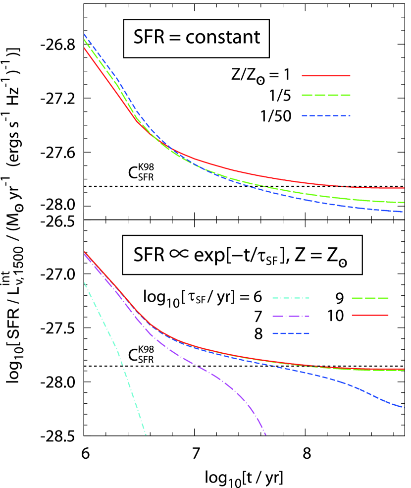
Figure 3.— Time evolution of $C_{\mathrm{SFR}}\equiv\mathrm{SFR}/L_{\nu,1500}^{\mathrm{int}}$ calculated using the population synthesis model of Schaerer (2003) with a Salpeter IMF in the mass range $0.1$–$60~{}M_{\odot}$. Top: $C_{\mathrm{SFR}}$ for constant star formation. The solid, long-dashed, and short-dotted curves are for the stellar metallicities $Z/Z_{\odot}=1,\ 1/5,$ and $1/50$, respectively. Bottom: $C_{\mathrm{SFR}}$ for exponentially decaying star formation with an $e$-folding time of $\tau_{\mathrm{SF}}$ in the case of $Z=Z_{\odot}$. The solid, long-dashed, short-dashed, long-dash-dotted, and short-dash-dotted curves are $C_{\mathrm{SFR}}$ at $\log_{10}{\left(\tau_{\mathrm{SF}}/\mathrm{yr}\right)}=10$, 9, 8, 7, and 6, respectively. The horizontal dotted line in all panels represents the most popular conversion factor utilized in observational studies given by Kennicutt (1998), $C_{\mathrm{SFR}}^{\mathrm{K98}}=1.4\times 10^{-28}\ M_{\odot}\ \mathrm{yr^{-1}\ (erg\ s^{-1}\ Hz^{-1})^{-1}}$.

Figure 3 shows the time evolution of $C_{\mathrm{SFR}}$ at $\lambda=1500$ Å for constant and exponentially decaying star formation histories (SFHs). It is calculated using the Schaerer (2003) population synthesis model, which is used in our model to calculate the UV continuum luminosity of galaxies. As the true SFR of a galaxy having $L_{\nu,\mathrm{UV}}^{\mathrm{int}}$ is represented by $C_{\mathrm{SFR}}\times L_{\nu,\mathrm{UV}}^{\mathrm{int}}$, the SFR estimated by $C_{\mathrm{SFR}}^{\mathrm{K98}}\times L_{\nu,\mathrm{UV}}^{\mathrm{int}}$ wrongly represents the true SFR in the case of $C_{\mathrm{SFR}}\neq C_{\mathrm{SFR}}^{\mathrm{K98}}$. When $C_{\mathrm{SFR}}^{\mathrm{K98}}$ is larger than $C_{\mathrm{SFR}}$, the SFR will be overestimated by a factor of $C_{\mathrm{SFR}}^{\mathrm{K98}}/C_{\mathrm{SFR}}$, and vice versa.

In the early phase of constant star formation, $C_{\mathrm{SFR}}$ is significantly larger than $C_{\mathrm{SFR}}^{\mathrm{K98}}$, up to $\gtrsim 1$ dex at age $\sim 1$ Myr even in the case of solar metallicity $Z_{\odot}$ as shown in the top panel of Figure 3. This is simply because $L_{\nu,\mathrm{UV}}^{\mathrm{int}}$ grows continuously as the number of massive stars with a lifetime of $\sim 100$ Myr increases before it reaches equilibrium, which corresponds to $C_{\mathrm{SFR}}^{\mathrm{K98}}$ for $Z=Z_{\odot}$. Therefore, adopting $C_{\mathrm{SFR}}^{\mathrm{K98}}$ for such young galaxies results in an underestimation of SFR for a given $L_{\nu,\mathrm{UV}}^{\mathrm{int}}$. The extent of the underestimation depends on age, metallicity, and wavelength. Conversely, we overestimate the SFR of a galaxy which is old enough to be in equilibrium and which has sub-solar metallicity by up to $\sim 0.2$ dex (a factor of $\sim 1.6$). This can be understood by the fact that lower metallicity stars are bluer; a smaller SFR is enough to produce a certain $L_{\nu,\mathrm{UV}}^{\mathrm{int}}$ compared to stars with larger metallicity. Adopting $C_{\mathrm{SFR}}^{\mathrm{K98}}$ for such evolved galaxies with sub-solar metallicity results in an overestimation of the SFR, the extent of the overestimation depending on metallicity and wavelength.

In the case of an exponentially decaying SFH, $C_{\mathrm{SFR}}$ is not constant even at later stages of star formation if the $e$-folding time $\tau_{\mathrm{SF}}$ is short (i.e., $\tau_{\mathrm{SF}}\lesssim 100$ Myr). Rather, it decreases progressively with time as shown in the bottom panels of Figure 3. This is because $L_{\nu,\mathrm{UV}}^{\mathrm{int}}$ does not decrease as fast with time as the SFR. Massive stars with a lifetime of $\sim 100$ Myr can contribute to $L_{\nu,\mathrm{UV}}^{\mathrm{int}}$ even after the star formation activity is quenched in $\tau_{\mathrm{SF}}$. The K98 SFR conversion method for galaxies where SFR decays quickly, like starbursts, results in either an underestimation or an overestimation of SFR.

$C_{\mathrm{SFR}}$ should be smaller than $C_{\mathrm{SFR}}^{\mathrm{K98}}$ for higher-$z$ galaxies if their UV luminosities reach equilibrium because such galaxies typically have sub-solar metallicity. However, if UV LF is dominated by young galaxies whose $L_{\nu,\mathrm{UV}}^{\mathrm{int}}$ is increasing, $C_{\mathrm{SFR}}$ should be larger than $C_{\mathrm{SFR}}^{\mathrm{K98}}$. Therefore, it is not straightforward to treat $C_{\mathrm{SFR}}$ for a high-$z$ universe. In this paper we investigate the redshift dependence of $C_{\mathrm{SFR}}$ in detail using the Mitaka model.

2.3. Correction of Interstellar Dust Attenuation

In order to utilize the UV luminosity of a galaxy as an SFR indicator, we need to correct for its interstellar dust attenuation. This leads to the most influential uncertainty in the estimation of the CSFRD. This is because the amount of interstellar dust and its attenuation are not easily measurable from UV data alone (e.g., Burgarella et al. 2005). Moreover, the commonly used dust attenuation curve rises toward shorter wavelengths. The required luminosity correction can reach $\gtrsim 0.5$ dex at UV wavelengths.

H04 adopted two independent dust obscuration correction methods for the various observed LFs: common and SFR-dependent obscuration corrections. In both methods, the obscuration correction treats the observed LFs as statistical quantities, that is, H04 implicitly assumed that the observationally bright galaxies are also the intrinsically brightest.

In the common obscuration correction, H04 adopted $A_{V}=0.52$ mag for stars; this is a typical obscuration for UV-selected local galaxies (see Section 2.2 of H04). For the dust attenuation curve, they adopted the starburst obscuration curve given by Calzetti et al. (2000) for all galaxies regardless of their luminosities and redshift. Under these assumptions, the attenuation in magnitude for the stellar continuum at a wavelength of 1500 Å is evaluated as $A_{1500}=1.33$ mag. However, the dust attenuation of high-$z$ galaxies is not necessarily the same as that of the local UV-selected galaxies.

In the SFR-dependent correction, the obscuration for the UV continuum at $\lambda_{\mathrm{UV}}$, $A_{\mathrm{UV}}$, of a galaxy with observable UV luminosity $L_{\nu,\mathrm{UV}}$ is obtained by solving the following transcendental equation numerically:

$$A_{\mathrm{UV}}=X(\lambda_{\mathrm{UV}})\log_{10}{\left(\frac{0.797\log_{10}{(L_{\nu,\mathrm{UV}})+0.318A_{\mathrm{UV}}+0.573}}{2.88}\right)};$$ (1)

where $X(1500~{}\mbox{\AA})=8.935$ in the case of the Calzetti attenuation curve. Figure 4 shows $A_{\mathrm{UV}}$ for both the SFR-dependent correction and the common correction as a function of observable absolute magnitude at $\lambda_{\mathrm{UV}}=1500$ Å.

Figure 4.— Interstellar dust attenuation at $\lambda=1500$ Å, $A_{1500}$, as a function of observable (i.e., with dust attenuation) absolute magnitude $M_{1500}$ adopted in H04. The thick curve is $A_{1500}$ for the case of the SFR-dependent obscuration correction, obtained by solving the transcendental Equation (1) numerically. The thin horizontal line represents $A_{1500}$ for the case of the common obscuration correction. $A_{1500}$ at $M_{1500}\gtrsim-16$ mag for the SFR-dependent correction is 0 by definition, as in H04.

As shown in Figure 4, H04 adopted $A_{1500}=0$ mag at $M_{1500}\gtrsim-16$ mag because the numerical solution of Equation (1) for $A_{\mathrm{UV}}$ becomes negative and this is physically meaningless.

Equation (1) was originally derived from an empirical relation between $E(B-V)_{\mathrm{gas}}$ and the far-IR (FIR) luminosity $L_{\mathrm{FIR}}$ for normal galaxies, blue compact galaxies, and starbursts at the local universe, in which brighter galaxies have larger obscuration (see references given in Section 2.2 of H04). However, the distribution of these galaxies in the $E(B-V)_{\mathrm{gas}}$–$L_{\mathrm{FIR}}$ plane has significant scatter around the empirical relation (see Figure 1 of Hopkins et al. 2001). Moreover, the numerical constant in the numerator of the right-hand side in Equation (1) contains the uncertainty in $\mathrm{SFR}/L_{\mathrm{FIR}}$ and $\mathrm{SFR}/L_{\nu,\mathrm{UV}}^{\mathrm{int}}$. Even if this obscuration correction method had been derived empirically in the local universe, we should examine its validity in the high-$z$ universe. Thus, we investigate here the redshift dependence of the mean of $A_{\mathrm{UV}}$ in detail.

HB06 adopted a different approach from to of H04 at $z<3$; they added the FIR measurements of the CSFRD to the obscuration-uncorrected UV data as an effective dust obscuration correction in order to avoid assumptions about the extent or form of the obscuration and variations due to possible luminosity bias in the UV-selected sample (see Section 2.2 of HB06). At $z>3$, where there is no reliable FIR measurement of the CSFRD, HB06 adopted the common obscuration correction as in H04. As we do not calculate IR emission in this paper, we cannot examine the validity of the HB06 method. However, we give a brief comment on the consistency with the HB06 CSFRD in Section 5.2.

3. Model Description

In order to examine the cause of the disagreement between the CSFRDs obtained in theoretical and observational studies, we utilize a mock catalog of galaxies generated by a semi-analytic model for galaxy formation called the Mitaka model (Kobayashi et al. 2007, 2010; updated version of Nagashima & Yoshii 2004). The Mitaka model follows the framework of the $\Lambda$CDM model of structure formation and calculates the redshift evolution of the physical quantities of each galaxy at any redshift via semi-analytic computation of the merger histories of dark matter halos and the evolution of baryon components within halos. The time evolution of baryon components within halos is followed using physically motivated phenomenological models for radiative cooling, star formation, supernova feedback, chemical enrichment of gas and stars, and galaxy mergers. As a result, various physical and observational properties such as the SFR and intrinsic and observable stellar continuum luminosities of the galaxies at any given redshift can be obtained.

A detailed description of our model is given in Nagashima & Yoshii (2004) and Kobayashi et al. (2007, 2010). Therefore, here we briefly describe some key prescriptions which are closely related to this paper. Then, we explain how to examine the origin of the difference in CSFRD between observation and theory by using the mock catalog of galaxies generated by the Mitaka model.

3.1. Merger Tree of Dark Matter Halos

The merger histories of dark matter halos are realized using a Monte Carlo method based on the extended Press-Schechter formalism (Bond et al. 1991; Bower 1991; Lacey & Cole 1993). For the halo mass function to provide the weight for summing merger trees, the Mitaka model adopts the analytic functional form given by Yahagi et al. (2004); this is a fitting function to their high-resolution $N$-body simulation.

Figure 5.— 1500 Å LFs (top) and LDs (bottom) as a function of absolute magnitude and limiting absolute magnitude for integration, respectively, at $z=0$. The thin solid and dotted curves are the intrinsic and observable quantities of the Mitaka model, respectively. The thick solid and dashed curves are the common and SFRdep LFs and LDs calculated by applying the common and SFR-dependent obscuration corrections of H04 to the observable LF of the Mitaka model.

Dark matter halos with circular velocity $V_{\mathrm{c}}\geq V_{\mathrm{low}}=30\ \mathrm{km\ s^{-1}}$ are regarded as isolated halos, corresponding to the lower limits of halo mass $M_{\mathrm{halo}}\gtrsim 10^{9}\ M_{\odot}$ and $10^{10}\ M_{\odot}$ at $z=5$ and 0, respectively. Because of the existence of $V_{\mathrm{low}}$, fainter galaxies (i.e., $M_{1500}\gtrsim-10$ mag) are not well resolved in the Mitaka model. However, this limited resolution does not affect the resulting quantities at 1500 Å, $\rho_{\mathrm{1500}}$ and $\dot{\rho}_{\star}$, because $M_{1500}\sim-10$ mag is much fainter than $M_{\ast}$ and $\rho_{\mathrm{1500}}$ converges well at magnitudes much brighter those shown in the bottom panel of Figure 5.

3.2. Stellar Continuum Luminosity

The intrinsic luminosities and colors of galaxies in our model are calculated according to their SFHs and chemical enrichment histories using a stellar population synthesis model. We emphasize that we do not assume a simple linear relation between the intrinsic luminosity and SFR even at UV wavelengths. While the original Mitaka model uses the population synthesis model of Kodama & Arimoto (1997), our model uses that of Schaerer (2003) to calculate the UV stellar continuum luminosity as in Kobayashi et al. (2007, 2010). Compared to the Kodama & Arimoto (1997) model, the Schaerer (2003) model is a more recent one and covers a wider range of metallicity (including zero metallicity).

It has already been shown (Kobayashi et al. 2007, 2010) that the revised version of the Mitaka model reproduces all well the observed statistical quantities of high-$z$ Ly$\alpha$ emitters and Lyman-break galaxies.

3.3. Prescription for Dust Attenuation

In order to calculate observational (i.e., with interstellar dust attenuation) luminosities and colors of model galaxies, we model the optical depth of their internal dust as follows. We make the usual assumption that dust abundance of a galaxy is proportional to its gas metallicity and that the dust optical depth $\tau_{\mathrm{d}}$ is proportional to the column density of metals:

$$\tau_{\mathrm{d}}\propto\frac{M_{\mathrm{c}}Z_{\mathrm{c}}}{r_{\mathrm{e}}^{2}},$$ (2)

where $M_{\mathrm{c}}$ and $Z_{\mathrm{c}}$ are the mass and metallicity of cold gas, respectively, and $r_{\mathrm{e}}$ is the effective radius, all of which are obtained in our model. The normalization of Equation (2) is assumed to be a constant and universal regardless of galaxy properties and redshift, and has been determined to fit the observed data of local galaxies.

The wavelength dependence of the dust optical depth $\tau_{\mathrm{d}}(\lambda)$ is adopted to be the same as the Galactic extinction curve given by Pei (1992). In terms of the dust distribution, our Mitaka model assumes slab geometry (i.e., a uniform distribution of sources and absorbers; see Equation (19) of Calzetti et al. 1994 or Section 3.2 of Clemens & Alexander 2004). Therefore, the amount of attenuation magnitude $A_{\lambda}$ for the stellar continuum is given by

$$10^{-0.4A_{\lambda}}=\frac{1-\exp{(-\tau_{\mathrm{d}}(\lambda))}}{\tau_{\mathrm{d}}(\lambda)}.$$ (3)

Note that, while the wavelength dependence of $A_{\lambda}$ calculated via Equation (3) is similar to that of $\tau_{\mathrm{d}}$ (i.e., the Galactic extinction curve) at $\tau_{\mathrm{d}}\ll 1$, they are significantly different at $\tau_{\mathrm{d}}\gg 1$: $A_{\lambda}$ becomes flatter than $\tau_{\mathrm{d}}$ at $\tau_{\mathrm{d}}\gg 1$ as $A_{\lambda}\propto\log_{10}{\tau_{\lambda}}$. Therefore, the wavelength dependence of $A_{\lambda}$ in our model at $\tau_{\mathrm{d}}\gg 1$ is significantly different from that of the Calzetti law.

We emphasize that our model calculates star formation and chemical enrichment consistently in the framework of hierarchical structure formation. Therefore, both the time evolution of $\tau_{\mathrm{d}}$ for each model galaxy and the redshift evolution of its mean at a certain redshift can be naturally incorporated into our model together with the evolution of $M_{\mathrm{c}}$, $Z_{\mathrm{c}}$ and $r_{\mathrm{e}}$.

3.4. Application to the CSFRD Study

In this paper, we calculate the CSFRD in the redshift range $z=0$–10 using the mock catalog of galaxies generated by our model following the prescriptions in H04. We treat the mock catalog like observational data compiled from the literature and utilized to obtain the CSFRD in H04. We emphasize the most striking difference between our catalog and the data compiled in H04 is that each model galaxy in our catalog has information on its intrinsic UV luminosity and SFR as well as the observable luminosity.

We apply the same obscuration corrections as H04 (i.e., common and SFR-dependent corrections) to the observable UV LFs at $z=0$–10 given by our model in order to obtain the intrinsic LFs, which are represented as common and SFRdep LFs, respectively. Their LDs are represented as $\rho_{\mathrm{UV}}^{\mathrm{com}}$ and $\rho_{\mathrm{UV}}^{\mathrm{SFRdep}}$, respectively. We note here that the observable UV LF given by our model can be separated into contributions from each model galaxy. Therefore, the intrinsic UV LF can be obtained directly by counting the contributions of model galaxies in each magnitude bin. However, we treat the observable UV LF as a statistical quantity to examine whether the H04 obscuration corrections reproduce the “true” intrinsic UV LF and $\rho_{\mathrm{UV}}^{\mathrm{int}}$.

The conversion factor $C_{\mathrm{SFR}}^{\mathrm{K98}}$ is also compared with that of our model both in each galaxy, $\mathrm{SFR}/L_{\nu,\mathrm{UV}}^{\mathrm{int}}$, and in all galaxies, $\dot{\rho}_{\star}/\rho_{\mathrm{UV}}^{\mathrm{int}}$. We note again that the intrinsic UV luminosity of a galaxy is calculated according to its detailed SFH and chemical enrichment history; therefore $C_{\mathrm{SFR}}$ can vary in every galaxy.

We note here that, while there are several free parameters in phenomenological models for baryon evolution, in our model, they have already been determined to fit the various observations of the local galaxies (i.e., B- and K-band LFs, neutral gas mass fraction, and the gas mass-to-luminosity ratio as a function of B-band luminosity) in Nagashima & Yoshii (2004). As we utilize the values from this work unchanged in our study, there are no free parameters that can be adjusted.

4. Comparison with H04 Prescriptions

4.1. Dust Obscuration Correction

We first show the results from the H04 approaches to correcting for interstellar dust obscuration. The intrinsic and observable UV LFs at $1500$ Å at $z=0$ are shown in the top panel of Figure 5.

The common and SFRdep LFs (top panel) and their LDs (bottom panel) are also shown. Both LDs agree with the intrinsic one if we integrate the LFs up to $\gtrsim-16$ mag, even though both LFs show a significant deviation from the intrinsic one. This might be trivial because both of the H04 corrections are calibrated by galaxies in the local universe.

Figure 6.— Distribution of model galaxies with $M_{1500}^{\mathrm{int}}\leq-15$ mag at $z=0$ in the $A_{1500}$–$M_{1500}$ plane. The color scale shows the color-coded values of the number density of model galaxies per unit area. The open circles with error bars connected by lines are the mean and $1\sigma$ for the model galaxies in each magnitude bin. The obscuration corrections of H04 are also shown as the solid curve and dotted line for the SFR dependent and common corrections, respectively. The dashed lines indicate the contours of $M_{1500}^{\mathrm{int}}$ corresponding to $-22$, $-20$, and $-18$ AB mag from left to right.

In order to see the origin of the similarities and discrepancies between the UV LF and LD given by our model and those using the H04 methods, we compare the dust attenuation of model galaxies as a function of absolute magnitude $M_{1500}$ with $A_{1500}^{\mathrm{com}}$ and $A_{1500}^{\mathrm{SFRdep}}$. As shown in Figure 6, the means of $A_{1500}$, $\langle A_{1500}\rangle$, for our model galaxies at each magnitude are found to be almost constant, $\langle A_{1500}\rangle\approx 0.6$–1.0 mag, for $-22~{}\mathrm{mag}\lesssim M_{1500}\lesssim-15$ mag. However, model galaxies with a certain magnitude have significant dispersion around $\langle A_{1500}\rangle$ up to $\sim 1.0$ mag. This means that a non-negligible number of intrinsically bright galaxies lies at observationally faint magnitudes. The contribution from such observationally faint and intrinsically bright galaxies to the intrinsic LF and LD is completely neglected if a single value of $\langle A_{1500}\rangle$ at a certain magnitude is adopted as the representative attenuation for all galaxies with this magnitude. Therefore, correcting for dust attenuation by using $\langle A_{1500}\rangle$ results in underestimation of the bright ends of the intrinsic LF and intrinsic LD.

Taking the consideration above into account, we compare the H04 obscuration corrections with the median quantity $\langle A_{1500}\rangle$ for the model galaxies. The attenuation in the common correction of $A_{1500}^{\mathrm{com}}=1.33$ mag is found to be larger than $\langle A_{1500}\rangle$ by $\approx 0.3$–0.7 mag, that is, within the 1$\sigma$ error except for the brightest magnitudes. As shown in the top panel of Figure 5, this overcorrection for dust attenuation compared to the correction with $\langle A_{1500}\rangle$ is not sufficient to compensate for the contribution of the observationally faint and intrinsically bright galaxies at the bright end of the intrinsic LF. However, the overcorrection at faint magnitudes is enough to cover the underestimation of the LD at the bright end. Hence, the common correction results in a similar intrinsic UV LD to that of the Mitaka model. On the other hand, attenuation in the SFR-dependent correction of $A_{1500}^{\mathrm{SFRdep}}$ is significantly different from $\langle A_{1500}\rangle$. We note that it is also different from the recent observational result for star-forming galaxies with $z=0.95$–2.2, which shows that the mean attenuation at far-UV wavelengths decreases toward the bright far-UV continuum luminosity (see Figure 7 of Buat et al. 2012). It is larger and smaller than $\langle A_{1500}\rangle$ in the magnitude range $M_{1500}\lesssim-18$ mag and $M_{1500}\gtrsim-18$ mag, respectively. The overcorrection at bright magnitudes leads to the overestimation of the bright end of the intrinsic LF as shown in Figure 5. It is compensated for by the underestimation of the number density of faint galaxies. As a result, the SFR-dependent correction also results in a similar intrinsic UV LD to that of the Mitaka model.

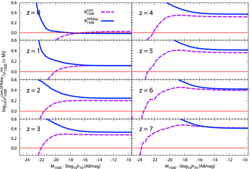
Figure 7.— LD ratios $R_{1500}^{\mathrm{com,SFRdep}}\equiv\rho_{1500}^{\mathrm{com,SFRdep}}/\rho_{1500}^{\mathrm{int}}$ as a function of absolute magnitude for the wavelength $\lambda=1500$ Å in the redshift range $z=0$–7 from top left to bottom right. The line styles are the same as in Figure 5.

We show the redshift evolution of the intrinsic 1500 Å LD ratios $R_{1500}^{i}\equiv\rho_{1500}^{i}/\rho_{1500}^{\mathrm{int}}$, where $i=\mathrm{com}$ or SFRdep, as a function of magnitude in Figure 7. As both correction methods ignore the contribution of observationally faint and intrinsically bright galaxies, the values of $R_{1500}^{i}$ depart significantly from unity at bright magnitudes. However, at faint magnitudes the $R_{1500}^{i}$ rapidly converge to the same value; the asymptotic values of $R_{1500}^{i}$ at $z=0$ are found to be unity, as seen in Figure 5. However, it is easily seen that the asymptotic values increase with $z$ and reach $\sim 0.3$ dex and $\sim 0.4$ dex at $z=3$ and $z\geq 4$, respectively. In summary, the H04 obscuration corrections alone result in the overestimation of CSFRD by $\sim 0.1$–0.4 dex in the redshift range $z=0$–10 compared to that of our model galaxies.

4.2. Ratio of UV Luminosity to SFR

In Figure 8, we show the distribution of model galaxies with $M_{1500}^{\mathrm{int}}\leq-15$ mag at $z=0$ in the $C_{\mathrm{SFR}}$–$M_{1500}$ plane. It is found there are two sequences in the plane: a constant sequence at $\sim C_{\mathrm{SFR}}^{\mathrm{K98}}$ and a widely spread sequence around the constant sequence with relatively high and low number densities ($\gtrsim 10^{-4}~{}h_{70}^{3}~{}\mathrm{Mpc^{-3}}$ and $\lesssim 10^{-6}~{}h_{70}^{3}~{}\mathrm{Mpc^{-3}}$), respectively. These sequences correspond to the two distinctive galaxy populations in our model, that is, quiescently star-forming and starburst galaxies, respectively.

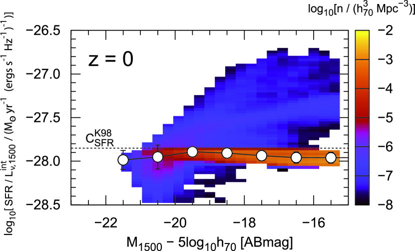
Figure 8.— Same as Figure 6, but for the distribution in the $C_{\mathrm{SFR}}$–$M_{1500}$ plane. $C_{\mathrm{SFR}}^{\mathrm{K98}}=1.4\times 10^{-28}\ M_{\odot}\ \mathrm{yr^{-1}\ (erg\ s^{-1}\ Hz^{-1})^{-1}}$ is also shown as a dotted horizontal.

The quiescent galaxies have long star formation timescales ($\gtrsim 1$ Gyr) and form disk stars almost constantly in the timestep of the Mitaka model. Therefore, the quantities contributing to $C_{\mathrm{SFR}}$ already reach equilibrium, with values depending on the stellar metallicity. As there is a well-known magnitude–metallicity relation (i.e., fainter galaxies have smaller metallicity; e.g., Garnett 2002), $C_{\mathrm{SFR}}$ decreases toward fainter magnitudes. In contrast, the starburst galaxies, whose starburst activity is triggered by a major merger of galaxies, have short star formation timescales ($\tau_{\mathrm{SF}}\lesssim 1$ Gyr) determined via the dynamical timescale of a newly formed spheroid. Because the starburst onset times are chosen randomly in the timestep of the Mitaka model, they have a variety of $C_{\mathrm{SFR}}$s according to the onset time and $\tau_{\mathrm{SF}}$ as shown in the bottom panel of Figure 3. The starburst galaxies whose $C_{\mathrm{SFR}}$ are larger than $C_{\mathrm{SFR}}^{\mathrm{K98}}$ are relatively young and those with $C_{\mathrm{SFR}}<C_{\mathrm{SFR}}^{\mathrm{K98}}$ are old enough to have such small $C_{\mathrm{SFR}}$.

We also evaluate the mean $C_{\mathrm{SFR}}$, $\langle C_{\mathrm{SFR}}\rangle$, for all our model galaxies at each magnitude. Starburst galaxies dominate the bright end in $M_{1500}$ at $z=0$ ($\lesssim-20$ mag) while quiescent galaxies determine $\langle C_{\mathrm{SFR}}\rangle$ except for the bright end. As a combination of the contributions from these two distinctive populations, $\langle C_{\mathrm{SFR}}\rangle$ is found to be almost constant in all of the magnitude range shown in Figure 8 and is always smaller than $C_{\mathrm{SFR}}^{\mathrm{K98}}$. Therefore, converting $L_{\nu,\mathrm{UV}}^{\mathrm{int}}$ into SFR via $C_{\mathrm{SFR}}^{\mathrm{K98}}$ results in an overestimation of the SFR for most galaxies at $z=0$, although the overestimation is not significant ($\lesssim 0.1$ dex).

Let us define the effective $L_{\nu,\mathrm{UV}}^{\mathrm{int}}$-to-SFR conversion factor, $C_{\mathrm{SFR}}^{\mathrm{eff}}(z)$, via:

$$C_{\mathrm{SFR}}^{\mathrm{eff}}(z)\equiv\dot{\rho}_{\star}(z)/\rho_{\mathrm{UV}}^{\mathrm{int}}(z).$$ (4)

This is not a conversion factor for each galaxy but by definition is the direct conversion from the statistical quantity of the intrinsic UV LD, $\rho_{\mathrm{UV}}^{\mathrm{int}}$, into the CSFRD, $\dot{\rho_{\star}}$. $\dot{\rho}_{\star}$ and $\rho_{\mathrm{UV}}^{\mathrm{int}}$ can be rewritten as summations of the contribution from each galaxy via $\dot{\rho}_{\star}=\sum\mathrm{SFR}^{i}=\sum(C_{\mathrm{SFR}}^{i}\times L_{\nu,1500}^{\mathrm{int},i})$ and $\rho_{\mathrm{UV}}^{\mathrm{int}}=\sum L_{\nu,1500}^{\mathrm{int},i}$, where the suffix $i$ indicates a galaxy. Hence, $C_{\mathrm{SFR}}^{\mathrm{eff}}=\sum(C_{\mathrm{SFR}}^{i}\times L_{\nu,1500}^{\mathrm{int},i})/\sum L_{\nu,1500}^{\mathrm{int},i}$ also represents a mean conversion factor of $C_{\mathrm{SFR}}$ weighted by the intrinsic UV continuum luminosity $L_{\nu,1500}^{\mathrm{int}}$. Figure 9 shows the redshift evolution of $C_{\mathrm{SFR}}^{\mathrm{eff}}(z)$ at $\lambda=1500$ Å.

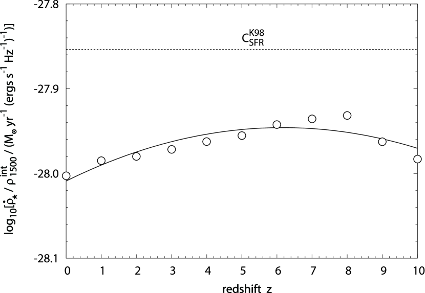
Figure 9.— Ratio of the CSFRD and intrinsic 1500 Å LD (i.e., $C_{\mathrm{SFR}}^{\mathrm{eff}}$) of the Mitaka model as a function of redshift. The open circles are the model results and the solid curve shows the best-fit quadratic function defined by Equation (9); the best-fit parameters are compiled in Table 2. Note that the dynamic range of the vertical axis (0.3 dex) is much smaller than that of Figure 8 (2.0 dex).

As shown in Figure 9, $C_{\mathrm{SFR}}^{\mathrm{eff}}$ at $z=0$ is smaller than $C_{\mathrm{SFR}}^{\mathrm{K98}}$ by $\sim 0.15$ dex. This result is natural because $\langle C_{\mathrm{SFR}}\rangle$ is smaller than $C_{\mathrm{SFR}}^{\mathrm{K98}}$ over the magnitude range $-22\ \mathrm{mag}\lesssim M_{1500}\lesssim-15$ mag as shown in Figure 8. This implies that converting $\rho_{\mathrm{UV}}^{\mathrm{int}}$ for the model galaxies at $z=0$ into $\dot{\rho}_{\star}$ using $C_{\mathrm{SFR}}^{\mathrm{K98}}$ overestimates $\dot{\rho}_{\star}$ compared to its true quantity by $\approx 0.15$ dex. The redshift evolution of $C_{\mathrm{SFR}}^{\mathrm{eff}}$ is also shown in Figure 9. It cannot be not simply understood because of the following effects. Toward high redshift, the contribution from young starbursts increases because of the increasing rate of the major merger. This effect results in an increase in $C_{\mathrm{SFR}}^{\mathrm{eff}}$. At the same time, the dynamical timescale of starburst galaxies becomes shorter at higher redshift because the galaxies formed tend to be smaller in size and hence have shorter $\tau_{\mathrm{SF}}$. This effect results in a decrease in $C_{\mathrm{SFR}}^{\mathrm{eff}}$ because $C_{\mathrm{SFR}}$ rapidly decays in galaxies with short $\tau_{\mathrm{SF}}$. These two competing effects lead to an increase in $C_{\mathrm{SFR}}^{\mathrm{eff}}$ toward $z\lesssim 8$ and its decrease at $z\gtrsim 8$.

$C_{\mathrm{SFR}}^{\mathrm{eff}}$ for $\lambda=1500$ Å is found to be always smaller than $C_{\mathrm{SFR}}^{\mathrm{K98}}$ by $\approx 0.10$–0.15 dex. The reason why $C_{\mathrm{SFR}}^{\mathrm{eff}}$ is always smaller than $C_{\mathrm{SFR}}^{\mathrm{K98}}$ is as follows. As shown in Figure 3, the time duration during which the galaxies have $C_{\mathrm{SFR}}$ larger than $C_{\mathrm{SFR}}^{\mathrm{K98}}$ is short ($\lesssim 100$ Myr) for any metallicity and for both constant and exponentially declining SFHs. This implies that the chance probability to detect a galaxy with $C_{\mathrm{SFR}}>C_{\mathrm{SFR}}^{\mathrm{K98}}$ is smaller than the probability to observe a galaxy with $C_{\mathrm{SFR}}<C_{\mathrm{SFR}}^{\mathrm{K98}}$. Moreover, high-$z$ galaxies tend to have a metallicity smaller than $Z_{\odot}$ and hence the equilibrium value of $C_{\mathrm{SFR}}$ is smaller than $C_{\mathrm{SFR}}^{\mathrm{K98}}$ for the constantly star-forming galaxies. As a consequence of these two reasons, the mean of $C_{\mathrm{SFR}}$ becomes smaller than $C_{\mathrm{SFR}}^{\mathrm{K98}}$ at all redshifts.

In summary, adopting the usual conversion factor of $C_{\mathrm{SFR}}^{\mathrm{K98}}$ for galaxies at $z=0$–10 results in an overestimation of $\dot{\rho}_{\star}$ by $\approx 0.10$–0.15 dex.

5. Summary and Discussion

In this paper, we examined the cause of the inconsistency in the CSFRD between theoretical and observational studies, focusing on an SFR indicator for a high-$z$ universe, that is, the rest-frame 1500 Å stellar continuum luminosity $L_{1500}$. By using a semi-analytic model for galaxy formation, the so-called Mitaka model, we found that the underestimation of the CSFRD seen in theoretical model originates from the following two uncertainties in the process to evaluate the CSFRD from the observed 1500 Å LD: the dust obscuration correction and the conversion from $L_{1500}$ to SFR. The uncertainty in the faint-end slope of the LF is not the origin of the underestimation of CSFRD but the origin of the dispersion around the median CSFRD. The methods of obscuration correction adopted in H04 result in the overestimation of the CSFRD by $\approx 0.1$–0.4 dex and the SFR conversion used in observational studies also leads to the overestimation of the CSFRD by $\approx 0.1$–0.2 dex.

Since theoretical models including ours reproduce the observed data for the UV LD which is not corrected by dust attenuation and the data for the SMD, the inconsistency in the CSFRD does not imply that theoretical models miss some key physical processes in galaxy formation. Of course, the theoretical models are not yet perfect because observed data such as cosmic downsizing (e.g., Cowie et al. 1996) remain to be reproduced. The revision of theoretical models can be achieved through a comparison with direct observed data which are not affected by a certain model and/or assumptions.

In this section, we provide a brief discussion of the origin of the difference in dust attenuation at high $z$ between our model and the H04 corrections. We also present new empirical calibrations for dust attenuation and SFR conversion as well as a recipe for utilizing them in observational studies.

5.1. Origin of the Difference in Dust Attenuation at High Redshift

As described in Section 4.1, the H04 obscuration correction methods reproduce the intrinsic LD from the observable UV LF of our model galaxies at $z=0$, although they overestimate it at higher redshifts. Here we discuss the origin of the overestimation at high redshift.

Our model naturally incorporates the redshift evolution of dust abundance because it calculates chemical enrichment of gas in each model galaxy consistently according to its SFH. This can be seen in Figure 10, which shows the redshift evolution of effective dust attenuation in magnitude, $A_{1500}^{\mathrm{eff}}$, for our model galaxies defined by

$$A_{1500}^{\mathrm{eff}}(z)\equiv-2.5\log_{10}{\left(\rho_{1500}(z)/\rho_{1500}^{\mathrm{int}}(z)\right)}.$$ (5)

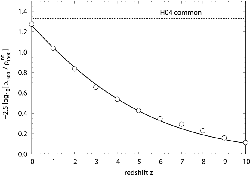
Figure 10.— Same as Figure 9, but for the ratio of the observable 1500 Å LD to the intrinsic one (i.e., $A_{1500}^{\mathrm{eff}}$) of the Mitaka model as a function of redshift. The parameters for the best-fit analytic function defined by Equation (8) and represented as the thick solid curve are also given in Table 2.

As $A_{1500}^{\mathrm{eff}}$ can be rewritten using the $A_{1500}$ and $L_{\nu,1500}^{\mathrm{int}}$ for each galaxy as $A_{1500}^{\mathrm{eff}}=-2.5\log_{10}(\sum(10^{-0.4A_{1500}^{i}}\times L_{\nu,1500}^{\mathrm{int},i})/$ $\sum L_{\nu,1500}^{\mathrm{int},i})$, $A_{1500}^{\mathrm{eff}}$ represents the mean dust attenuation weighted by the intrinsic UV continuum luminosity $L_{\nu,1500}^{\mathrm{int}}$. This is the reason why $A_{1500}^{\mathrm{eff}}$ at $z=0$ ($=1.3$ mag) is larger than $\langle A_{1500}\rangle$ at $z=0$ ($\lesssim 1$ mag). $A_{1500}^{\mathrm{eff}}$ becomes smaller at higher $z$ because of the redshift evolution of metallicity and dust abundance. However, such a redshift evolution of dust abundance is not incorporated into the H04 obscuration corrections. This is the origin of their overestimation of the intrinsic LD.

A quantity similar to $A_{1500}^{\mathrm{eff}}$ has been evaluated from the observed LD ratio between IR and UV, $\rho_{\mathrm{IR}}/\rho_{\mathrm{UV}}$ ($\approx\rho_{1500}^{\mathrm{int}}/\rho_{1500}-1$), in the redshift range $z=0$–1 (Takeuchi et al. 2005). They found that $A_{1500}^{\mathrm{eff}}$ increases monotonically toward $z=1$, which is the opposite trend to our result. However, more recent observational estimates for $\rho_{\mathrm{IR}}$ (e.g., Murphy et al. 2011; Casey et al. 2012; Cucciati et al. 2012) find that the redshift evolution of $\rho_{\mathrm{IR}}$ in this redshift range is milder than that reported by Takeuchi et al. (2005). Cucciati et al. (2012) also find that mean dust attenuation decreases toward high $z$ at $z\gtrsim 1$; their result is consistent with our prediction. These results may indicate that our model does not underestimate dust attenuation of galaxies at $z\gtrsim 1$ but overestimates it at $z\approx 0$. This interpretation will be examined as in our future work.

5.2. Comparison with the HB06 CSFRD

As described in Section 2.3, HB06 obtained the CSFRD at $z<3$ by summing the UV data and FIR measurements. They reported that this technique of UV$+$FIR measurements gives an effective obscuration correction to the UV data by a factor of 2 at $z\approx 0$ and $\sim 5$ (i.e., 1.7 mag) at $z\gtrsim 1$. It may be difficult to reconcile this with our result and should be examined in detail.

However, the correction factor of $\sim 5$ at $z\gtrsim 1$ reported in HB06 might be overestimated for the following reason. HB06 performed the effective obscuration correction by just adding a constant CSFRD measured by Le Floc’h et al. (2005) for FIR wavelengths at $z=1$. This is based on the observational result that FIR measurements of the CSFRD are quite flat in the range $z=1$–3 as reported by Pérez-González et al. (2005), who estimated the total IR luminosity of each galaxy by using the local template spectral energy distribution of Chary & Elbaz (2001). However, as reported by Murphy et al. (2011), using this template results in an overestimation of the total IR luminosity for IR-bright galaxies at $z>1.5$. Hence, the IR measurement of Pérez-González et al. (2005) may be overestimated. We are planning to investigate whether our model reproduces the observed IR data in future studies.

5.3. Empirical Calibrations of the Obscuration Correction and the SFR Conversion from UV Luminosity

Here we propose new empirical formulas which correct for dust obscuration and convert from the intrinsic UV LD, $\rho_{\mathrm{UV}}^{\mathrm{int}}$, to the CSFRD, $\dot{\rho}_{\star}$. These formulas are derived to reproduce the true quantities for the model galaxies and are represented by explicit analytic functions. For the obscuration correction, we show two different formulas; one is for the observable LF and the other is for its integrated quantity $\rho_{\mathrm{UV}}$. These two formulas are, respectively, similar to the SFR-dependent and common corrections of H04, but they are described to have redshift dependence.

5.3.1 Conversion from Observable LF into Intrinsic LF

Let us define $C_{\mathrm{dust}}$ as an empirical formula to convert the observable LF into an intrinsic one. $C_{\mathrm{dust}}$ at a certain magnitude $M_{1500}$ is determined via an abundance-matching approach. That is, the cumulative number density of the observable LF of the Mitaka model, $n^{\mathrm{obs}}(<M_{1500})$, should match that of the intrinsic LF, $n^{\mathrm{int}}(<M_{1500}-C_{\mathrm{dust}})$:

$$n^{\mathrm{obs}}(<M_{1500})=n^{\mathrm{int}}(<M_{1500}-C_{\mathrm{dust}}).$$ (6)

The top panel of Figure 11 shows the resultant $C_{\mathrm{dust}}$ as a function of $M_{1500}$ at $z=0$.

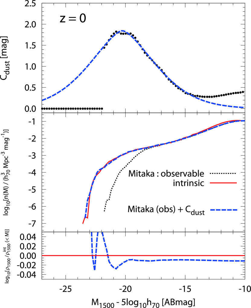
Figure 11.— Top, middle, and bottom panels show $C_{\mathrm{dust}}$, LF, and the ratio of the LD calculated from the Mitaka observable LF $+C_{\mathrm{dust}}$ to the Mitaka intrinsic LD, respectively, at $z=0$ for a wavelength of $\lambda=1500$ Å. In the top panel, the filled circles are the numerical data calculated from the intrinsic and observable 1500 Å LFs of the Mitaka model, while the dashed curve is analytical fit using Equation (7) with the numerical quantities in Table 1. $C_{\mathrm{dust}}=0$ at $M_{1500}\lesssim-22$ mag is reflected by the fact that there is no model galaxy with such bright observable magnitudes. In the middle panel, the solid and dotted curves are the intrinsic and observable LFs of the Mitaka model, respectively, while the dashed curve is the Mitaka observable LF + $C_{\mathrm{dust}}$.

We have derived $C_{\mathrm{dust}}$ for other redshifts and found that $C_{\mathrm{dust}}$ can be fitted well with the following analytic function in the redshift range $z=0$–10:

$$C_{\mathrm{dust}}(M_{1500};\ z)=a\ \exp{\left[-b|M_{1500}-M_{1500}^{0}|^{c}\right]}.$$ (7)

Here $a,\ b,\ c,$ and $M_{1500}^{0}$ are model parameters and evolve with redshift. $a$ and $M_{1500}^{0}$ have units of magnitude, while $b$ and $c$ are non-dimensional constants. We adopt a smoothly declining functional form even for the bright magnitudes where there are no model galaxies. We note that $C_{\mathrm{dust}}$ is a dust obscuration correction for the UV LF as a statistical quantity like the SFR-dependent correction of H04. Hence it does not represent a mean dust attenuation for the galaxies at a certain magnitude. Actually, the intrinsically UV-brightest galaxies are not the observationally brightest galaxies in our model, as described in Section 4.1. The reason why $C_{\mathrm{dust}}$ has a peak around the characteristic magnitude $M_{1500}^{\ast}$ is that the magnitude difference between the intrinsic and observable UV LFs becomes largest at $M_{1500}\approx M_{1500}^{\ast}$, not that the mean attenuation of the galaxies at $M_{1500}\approx M_{1500}^{\ast}$ is the largest.

There are significant discrepancies between the raw $C_{\mathrm{dust}}$ quantities and that evaluated using Equation (7), as represented by the filled circles and dashed curve, respectively, in the top panel of Figure 11 at $M_{1500}\lesssim-23$ mag or $M_{1500}\gtrsim-15$ mag. Fortunately, this deviation hardly affects the corrected UV LF or the integrated LD as shown in the middle and bottom panels of Figure 11. Table 1 gives the numerical quantities for the best-fit parameters in the redshift range $z=0$–10.

Table 1Fitting Parameters for our Formula to Correct Dust Attenuation, $C_{\mathrm{dust}}$

Redshift, $z$	$a$	$b$	$c$	$M_{1500}^{0}$
	(mag)			(mag)
0	$1.847$	$0.1139$	$1.566$	$-19.49$
1	$2.466$	$0.1181$	$1.281$	$-22.65$
2	$2.344$	$0.2625$	$1.086$	$-21.86$
3	$2.235$	$0.2844$	$1.184$	$-21.91$
4	$2.032$	$0.2115$	$1.428$	$-22.15$
5	$1.822$	$0.1971$	$1.599$	$-22.16$
6	$1.583$	$0.1673$	$1.737$	$-22.14$
7	$1.496$	$0.1630$	$1.800$	$-22.08$
8	$1.415$	$0.1900$	$1.641$	$-22.16$
9	$1.228$	$0.1239$	$1.895$	$-22.39$
10	$1.109$	$0.1898$	$1.634$	$-22.17$

Note. — The analytic expression for $C_{\mathrm{dust}}$ is given by Equation (7).

Table 2Fitting Parameters for our Formulas for $C_{\mathrm{dust}}^{\mathrm{eff}}$ and $C_{\mathrm{SFR}}^{\mathrm{eff}}$

$C_{\mathrm{dust}}^{\mathrm{eff}}$			$C_{\mathrm{SFR}}^{\mathrm{eff}}$
$\alpha$	$\beta$		$C_{2}$	$C_{1}$	$C_{0}$
					($M_{\odot}\ \mathrm{yr^{-1}\ (ergs/s/Hz)^{-1}}$)
$2.983$	$0.3056$		$-5.915\times 10^{-5}$	$7.294\times 10^{-4}$	$-28.01$

Note. — The analytic expressions for $C_{\mathrm{dust}}^{\mathrm{eff}}$ and $C_{\mathrm{SFR}}^{\mathrm{eff}}$ are given by Equations (8) and (9), respectively.

The normalization factor $a$ indicates the maximum value of $C_{\mathrm{dust}}$ at the redshift. $a$ is found to gradually increase with redshift toward its peak at $z\simeq 1$–3 and then decreases as $z$ increases. It is interesting that the peak redshift for $a$ is roughly equal to the redshift where dusty galaxies (e.g., ultraluminous infrared galaxies, sub-mm galaxies, etc.) are mainly found.

5.3.2 Conversion from Observable UV LD into Intrinsic UV LD

The conversion factor from the observed 1500 Å LD, $\rho_{1500}$, into the intrinsic one, $\rho_{1500}^{\mathrm{int}}$, is defined as $C_{\mathrm{dust}}^{\mathrm{eff}}\equiv\rho_{1500}^{\mathrm{int}}/\rho_{1500}$. This relates to the effective dust attenuation $A_{1500}^{\mathrm{eff}}$ defined in Equation (5) via $C_{\mathrm{dust}}^{\mathrm{eff}}=\mathrm{dex}(0.4A_{1500}^{\mathrm{eff}})$. It is found that the $C_{\mathrm{dust}}^{\mathrm{eff}}$ for our model galaxies can be well fitted by the following simple analytic function with two redshift-independent parameters $\alpha$ and $\beta$ in the redshift range $z=0$–10 as shown in Figure 10:

$$C_{\mathrm{dust}}^{\mathrm{eff}}(z)=\alpha\ \exp{\left[-\beta\left(1+z\right)\right]}+1.$$ (8)

This functional form is motivated by the natural expectation that $C_{\mathrm{dust}}^{\mathrm{eff}}$ approaches unity at high redshift. Since there is little dust at high redshift, $C_{\mathrm{dust}}^{\mathrm{eff}}\approx 1$. The best-fit parameters which reproduce the ratio $\rho_{1500}^{\mathrm{int}}/\rho_{1500}$ at $z=0$–10 within $\pm 10\%$ are given in Table 2.

While the normalization parameter $a$ in Equation (7) has its peak at $z\simeq 1$–3, $C_{\mathrm{dust}}^{\mathrm{eff}}$ decreases monotonically with increasing $z$. The different redshift evolution can be interpreted by the fact that the contribution from galaxies fainter than $M_{1500}^{0}$, where the galaxies have a maximum extinction of $a$ at the redshift, to the intrinsic 1500 Å LD is significant; for a typical faint-end slope $\alpha\approx-1.4$ of the UV LF, the contribution from galaxies with $L\lesssim L_{\ast}$ reaches $\sim 0.7$ dex as shown in the right panel of Figure 2. Since such faint galaxies have smaller $C_{\mathrm{dust}}$ than its peak value of $a$, $C_{\mathrm{dust}}^{\mathrm{eff}}$ progressively decreases toward high redshift although $a$ has its peak at $z\simeq 1$–3.

5.3.3 Conversion from Intrinsic UV LD into CSFRD

We find that the ratio of the CSFRD to the intrinsic 1500 Å LD, $\dot{\rho}_{\star}/\rho_{1500}^{\mathrm{int}}$, can be well fitted with the following simple quadratic function in the redshift range $z=0$–10:

$$C_{\mathrm{SFR}}^{\mathrm{eff}}(z)=C_{0}\left[1+C_{1}\left(1+z\right)+C_{2}\left(1+z\right)^{2}\right].$$ (9)

Here $C_{0},\ C_{1},$ and $C_{2}$ are the model parameters and are redshift-independent constants. $C_{0}$ has the same dimensions as $C_{\mathrm{SFR}}^{\mathrm{eff}}$, $M_{\odot}\ \mathrm{yr^{-1}\ (erg\ s^{-1}\ Hz^{-1})^{-1}}$, while $C_{1}$ and $C_{2}$ are non-dimensional constants. With the best-fit quantities given in Table 2, the analytic function reproduces our model results for $\dot{\rho}_{\star}/\rho_{1500}^{\mathrm{int}}$ within $\pm 5$%.

We note here that, while the empirical formula given in Equation (9) predicts that $C_{\mathrm{SFR}}^{\mathrm{eff}}$ has a peak at $z\sim 6$ and progressively decreases toward high redshifts, it is simply a fitting result and does not have any physical motivation. Nevertheless, it might be a real trend as discussed in Section 4.2.

5.4. Recipe for Converting Observed UV LF into CSFRD

Here we describe a recipe for converting the observed 1500 Å LF into the CSFRD $\dot{\rho}_{\star}$ using our empirical formulas given in Section 5.3. As a first step, the intrinsic 1500 Å LD, $\rho_{1500}^{\mathrm{int}}$, should be calculated from the observed UV LF. This can be done using either one of the following two approaches. The first approach is to convert the observed UV LF into an intrinsic LF via the empirical formula for $C_{\mathrm{dust}}$ as a function of magnitude and redshift given in Equation (7) with the best-fit parameters in Table 1. Then the intrinsic UV LF is integrated over magnitude to obtain the intrinsic UV LD, $\rho_{1500}^{\mathrm{int}}$. The second approach is to first integrate the observed UV LF over magnitude to obtain the observable UV LD, $\rho_{1500}$, and then converted it into $\rho_{1500}^{\mathrm{int}}$ using the empirical formula for $C_{\mathrm{dust}}^{\mathrm{eff}}$ as a function of redshift given in Equation (8). Finally, one can evaluate $\dot{\rho}_{\star}$ from $\rho_{1500}^{\mathrm{int}}$ using the empirical formula for $C_{\mathrm{SFR}}^{\mathrm{eff}}$ as a function of redshift given in Equation (9).

For $C_{\mathrm{dust}}$ given in Equation (7), it is statistically enough to linearly interpolate the formula for a specified redshift while the best-fit parameters are provided discretely in redshift for our empirical formula. One should interpolate the parameters to evaluate an adequate $C_{\mathrm{dust}}$ at a certain magnitude and the desired redshift rather than interpolating $C_{\mathrm{dust}}$ itself.

Table 3LD and CSFRD of the Mitaka Model

Redshift, $z$	$\dot{\rho_{\star}}$	$\rho_{1500}$	$\rho_{1500}^{\mathrm{int}}$	$\dot{\rho_{\star}}/\rho_{1500}$
	$(h_{70}\ M_{\odot}\ \mathrm{yr^{-1}\ Mpc^{-3}})$	$(h_{70}\ \mathrm{erg\ s^{-1}\ Hz^{-1}\ Mpc^{-3}})$	$(h_{70}\ \mathrm{erg\ s^{-1}\ Hz^{-1}\ Mpc^{-3}})$	$(M_{\odot}\ \mathrm{yr^{-1}\ (erg\ s^{-1}\ Hz^{-1})^{-1}})$
0	$2.599\times 10^{-2}$	$8.090\times 10^{25}$	$2.616\times 10^{26}$	$3.213\times 10^{-28}$
1	$6.825\times 10^{-2}$	$2.531\times 10^{26}$	$6.593\times 10^{26}$	$2.697\times 10^{-28}$
2	$8.285\times 10^{-2}$	$3.665\times 10^{26}$	$7.910\times 10^{26}$	$2.261\times 10^{-28}$
3	$6.828\times 10^{-2}$	$3.498\times 10^{26}$	$6.396\times 10^{26}$	$1.952\times 10^{-28}$
4	$4.926\times 10^{-2}$	$2.752\times 10^{26}$	$4.518\times 10^{26}$	$1.790\times 10^{-28}$
5	$3.124\times 10^{-2}$	$1.902\times 10^{26}$	$2.818\times 10^{26}$	$1.642\times 10^{-28}$
6	$1.759\times 10^{-2}$	$1.119\times 10^{26}$	$1.540\times 10^{26}$	$1.572\times 10^{-28}$
7	$9.105\times 10^{-3}$	$5.988\times 10^{25}$	$7.849\times 10^{25}$	$1.521\times 10^{-28}$
8	$4.524\times 10^{-3}$	$3.129\times 10^{25}$	$3.865\times 10^{25}$	$1.446\times 10^{-28}$
9	$2.069\times 10^{-3}$	$1.641\times 10^{25}$	$1.898\times 10^{25}$	$1.261\times 10^{-28}$
10	$9.514\times 10^{-4}$	$8.245\times 10^{24}$	$9.150\times 10^{24}$	$1.154\times 10^{-28}$

Note. — $\dot{\rho}_{\star}$ is the CSFRD and $\rho_{1500}$ and $\rho_{1500}^{\mathrm{int}}$ represent the observable and intrinsic 1500 Å LDs, respectively, for all of the galaxies in the Mitaka model.

Table 4CSFRD Parametric Fits to Various Forms from the Literatures

Reference	Functional Form	Parameter	Value
Cole et al. (2001)	$\dot{\rho}_{\ast}(z)=\left(a+bz\right)h\ /\ [1+\left(z/c\right)^{d}]$	$a$	$0.0389$
		$b$	$0.0545$
		$c$	$2.973$
		$d$	$3.655$
Hernquist & Springel (2003)	$\dot{\rho}_{\ast}(z)=\dot{\rho}_{0}\chi^{2}\ /\ [1+\alpha(\chi-1)^{3}\exp{(\beta\chi^{7/4})}]$	$\dot{\rho}_{0}$	$0.030$
	$\chi=[H(z)/H_{0}]^{2/3}$	$\alpha$	$0.323$
		$\beta$	$0.051$
Yüksel et al. (2008)	$\dot{\rho}_{\ast}(z)=\dot{\rho}_{0}[(1+z)^{\alpha\eta}+\{(1+z)/B\}^{\beta\eta}+\{(1+z)/C\}^{\gamma\eta}]^{1/\eta}$,	$\dot{\rho}_{0}$	$0.0258$
	$B=(1+z_{1})^{1-\alpha/\beta}$, string$C=(1+z_{1})^{(\beta-\alpha)/\gamma}(1+z_{2})^{1-\beta/\gamma}$	$\alpha$	$1.6$
		$\beta$	$-1.2$
		$\gamma$	$-5.7$
		$z_{1}$	$1.7$
		$z_{2}$	$5.0$
		$\eta$	$-1.62$

The numerical quantities for $\dot{\rho}_{\star},\ \rho_{1500},$ and $\rho_{1500}^{\mathrm{int}}$ of the Mitaka model are compiled in Table 3. We also present the CSFRD parametric fits to a variety of analytic forms in the literature (Cole et al. 2001; Hernquist & Springel 2003; Yüksel et al. 2008) in Table 4.

References

- Benson (2012) Benson, A. J. 2012, NewA, 17, 175
- Bond et al. (1991) Bond, J. R., Cole, S., Efstathiou, G., & Kaiser, N. 1991, ApJ, 379, 440
- Botticella et al. (2012) Botticella, M. T., Smartt, S. J., Kennicutt, R. C., Jr., et al. 2012, A&A, 537, A132
- Bower (1991) Bower, R. 1991, MNRAS, 248, 332
- Buat et al. (2012) Buat, V., Noll, S., Burgarella, D., et al. 2012, A&A, 545, A141
- Burgarella et al. (2005) Burgarella, D., Buat, V., & Iglesias-Páramo 2005, MNRAS, 360, 1413
- Calzetti et al. (2000) Calzetti, D., Armus, L., Bohlin, R. C., et al. 2000, ApJ, 533, 682
- Calzetti et al. (1994) Calzetti, D., Kinney, A. L., & Storchi-Bergmann, T. 1994, ApJ, 429, 582
- Casey et al. (2012) Casey, C. M., Berta, S., Béthermin, M., et al. 2012, ApJ, 761, 140
- Chary & Elbaz (2001) Chary, R. & Elbaz, Z. 2001, ApJ, 556, 562
- Choi & Nagamine (2011) Choi, J.-H., & Nagamine, K. 2012, MNRAS, 419, 1280
- Clemens & Alexander (2004) Clemens, M. S. & Alexander, P. 2004, MNRAS, 350, 66
- Cole et al. (2001) Cole, S., Norberg, P., Baugh, C. M., et al. 2001, MNRAS, 326, 255
- Coward et al. (2008) Coward, D. M., Guetta, D., Burman, R. R., & Imerito, A. 2008, MNRAS, 386, 111
- Cowie et al. (1996) Cowie, L. L., Songaila, A., Hu, E. M., & Cohen, J. G. 1996, AJ, 112, 839
- Cucciati et al. (2012) Cucciati, O., Tresse, L., Ilbert, O., et al. 2012, A&A, 539, 31
- Fioc & Rocca-Volmerange (1997) Fioc, M., & Rocca-Volmerange, B. 1997, A&A, 326, 950
- Garnett (2002) Garnett, D. R. 2002, ApJ, 581, 1019